| Issue |
A&A
Volume 694, February 2025
|
|
|---|---|---|
| Article Number | A141 | |
| Number of page(s) | 27 | |
| Section | Cosmology (including clusters of galaxies) | |
| DOI | https://doi.org/10.1051/0004-6361/202452018 | |
| Published online | 10 February 2025 | |
Euclid preparation
LIX. Angular power spectra from discrete observations
1
Department of Physics and Astronomy, University College London, Gower Street, London WC1E 6BT, UK
2
Oskar Klein Centre for Cosmoparticle Physics, Department of Physics, Stockholm University, Stockholm SE-106 91, Sweden
3
Astrophysics Group, Blackett Laboratory, Imperial College London, London SW7 2AZ, UK
4
Institute for Astronomy, University of Edinburgh, Royal Observatory, Blackford Hill, Edinburgh EH9 3HJ, UK
5
European Space Agency/ESTEC, Keplerlaan 1, 2201 AZ Noordwijk, The Netherlands
6
Institute Lorentz, Leiden University, Niels Bohrweg 2, 2333 CA Leiden, The Netherlands
7
Institut de Recherche en Astrophysique et Planétologie (IRAP), Université de Toulouse, CNRS, UPS, CNES, 14 Av. Edouard Belin, 31400 Toulouse, France
8
Mullard Space Science Laboratory, University College London, Holmbury St Mary, Dorking, Surrey RH5 6NT, UK
9
School of Mathematics and Physics, University of Surrey, Guildford, Surrey GU2 7XH, UK
10
INAF-Osservatorio Astronomico di Brera, Via Brera 28, 20122 Milano, Italy
11
INAF-Osservatorio di Astrofisica e Scienza dello Spazio di Bologna, Via Piero Gobetti 93/3, 40129 Bologna, Italy
12
IFPU, Institute for Fundamental Physics of the Universe, Via Beirut 2, 34151 Trieste, Italy
13
INAF-Osservatorio Astronomico di Trieste, Via G. B. Tiepolo 11, 34143 Trieste, Italy
14
INFN, Sezione di Trieste, Via Valerio 2, 34127 Trieste, TS, Italy
15
SISSA, International School for Advanced Studies, Via Bonomea 265, 34136 Trieste, TS, Italy
16
Dipartimento di Fisica e Astronomia, Università di Bologna, Via Gobetti 93/2, 40129 Bologna, Italy
17
INFN-Sezione di Bologna, Viale Berti Pichat 6/2, 40127 Bologna, Italy
18
Institut de Physique Théorique, CEA, CNRS, Université Paris-Saclay, 91191 Gif-sur-Yvette Cedex, France
19
Institut d’Astrophysique de Paris, UMR 7095, CNRS, and Sorbonne Université, 98 bis Boulevard Arago, 75014 Paris, France
20
INAF-Osservatorio Astrofisico di Torino, Via Osservatorio 20, 10025 Pino Torinese, TO, Italy
21
Dipartimento di Fisica, Università di Genova, Via Dodecaneso 33, 16146 Genova, Italy
22
INFN-Sezione di Genova, Via Dodecaneso 33, 16146 Genova, Italy
23
Department of Physics “E. Pancini”, University Federico II, Via Cinthia 6, 80126 Napoli, Italy
24
INAF-Osservatorio Astronomico di Capodimonte, Via Moiariello 16, 80131 Napoli, Italy
25
INFN Section of Naples, Via Cinthia 6, 80126 Napoli, Italy
26
Instituto de Astrofísica e Ciências do Espaço, Universidade do Porto, CAUP, Rua das Estrelas, PT4150-762 Porto, Portugal
27
Faculdade de Ciências da Universidade do Porto, Rua do Campo de Alegre, 4150-007 Porto, Portugal
28
Aix-Marseille Université, CNRS, CNES, LAM, Marseille, France
29
Dipartimento di Fisica, Università degli Studi di Torino, Via P. Giuria 1, 10125 Torino, Italy
30
INFN-Sezione di Torino, Via P. Giuria 1, 10125 Torino, Italy
31
INAF-IASF Milano, Via Alfonso Corti 12, 20133 Milano, Italy
32
INAF-Osservatorio Astronomico di Roma, Via Frascati 33, 00078 Monteporzio Catone, Italy
33
INFN-Sezione di Roma, Piazzale Aldo Moro, 2 – c/o Dipartimento di Fisica, Edificio G. Marconi, 00185 Roma, Italy
34
Centro de Investigaciones Energéticas, Medioambientales y Tecnológicas (CIEMAT), Avenida Complutense 40, 28040 Madrid, Spain
35
Port d’Informació Científica, Campus UAB, C. Albareda s/n, 08193 Bellaterra, (Barcelona), Spain
36
Institute for Theoretical Particle Physics and Cosmology (TTK), RWTH Aachen University, 52056 Aachen, Germany
37
Institute of Cosmology and Gravitation, University of Portsmouth, Portsmouth PO1 3FX, UK
38
Dipartimento di Fisica e Astronomia “Augusto Righi” – Alma Mater Studiorum Università di Bologna, Viale Berti Pichat 6/2, 40127 Bologna, Italy
39
Instituto de Astrofísica de Canarias, Calle Vía Láctea s/n, 38204 San Cristóbal de La Laguna, Tenerife, Spain
40
Jodrell Bank Centre for Astrophysics, Department of Physics and Astronomy, University of Manchester, Oxford Road, Manchester M13 9PL, UK
41
European Space Agency/ESRIN, Largo Galileo Galilei 1, 00044 Frascati, Roma, Italy
42
ESAC/ESA, Camino Bajo del Castillo, s/n, Urb. Villafranca del Castillo, 28692 Villanueva de la Cañada, Madrid, Spain
43
Université Claude Bernard Lyon 1, CNRS/IN2P3, IP2I Lyon, UMR 5822, Villeurbanne F-69100, France
44
Institute of Physics, Laboratory of Astrophysics, Ecole Polytechnique Fédérale de Lausanne (EPFL), Observatoire de Sauverny, 1290 Versoix, Switzerland
45
Institut de Ciències del Cosmos (ICCUB), Universitat de Barcelona (IEEC-UB), Martí i Franquès 1, 08028 Barcelona, Spain
46
Institució Catalana de Recerca i Estudis Avançats (ICREA), Passeig de Lluís Companys 23, 08010 Barcelona, Spain
47
UCB Lyon 1, CNRS/IN2P3, IUF, IP2I Lyon, 4 Rue Enrico Fermi, 69622 Villeurbanne, France
48
Departamento de Física, Faculdade de Ciências, Universidade de Lisboa, Edifício C8, Campo Grande, PT1749-016 Lisboa, Portugal
49
Instituto de Astrofísica e Ciências do Espaço, Faculdade de Ciências, Universidade de Lisboa, Campo Grande, 1749-016 Lisboa, Portugal
50
Department of Astronomy, University of Geneva, Ch. d’Ecogia 16, 1290 Versoix, Switzerland
51
INFN-Padova, Via Marzolo 8, 35131 Padova, Italy
52
INAF-Istituto di Astrofisica e Planetologia Spaziali, Via del Fosso del Cavaliere, 100, 00100 Roma, Italy
53
Université Paris-Saclay, Université Paris Cité, CEA, CNRS, AIM, 91191 Gif-sur-Yvette, France
54
Space Science Data Center, Italian Space Agency, Via del Politecnico snc, 00133 Roma, Italy
55
Aix-Marseille Université, CNRS/IN2P3, CPPM, Marseille, France
56
Istituto Nazionale di Fisica Nucleare, Sezione di Bologna, Via Irnerio 46, 40126 Bologna, Italy
57
FRACTAL S.L.N.E., Calle Tulipán 2, Portal 13 1A, 28231 Las Rozas de Madrid, Spain
58
INAF-Osservatorio Astronomico di Padova, Via dell’Osservatorio 5, 35122 Padova, Italy
59
Max Planck Institute for Extraterrestrial Physics, Giessenbachstr. 1, 85748 Garching, Germany
60
Universitäts-Sternwarte München, Fakultät für Physik, Ludwig-Maximilians-Universität München, Scheinerstrasse 1, 81679 München, Germany
61
Dipartimento di Fisica “Aldo Pontremoli”, Università degli Studi di Milano, Via Celoria 16, 20133 Milano, Italy
62
Institute of Theoretical Astrophysics, University of Oslo, PO Box 1029 Blindern, 0315 Oslo, Norway
63
Leiden Observatory, Leiden University, Einsteinweg 55, 2333 CC Leiden, The Netherlands
64
Jet Propulsion Laboratory, California Institute of Technology, 4800 Oak Grove Drive, Pasadena, CA 91109, USA
65
Felix Hormuth Engineering, Goethestr. 17, 69181 Leimen, Germany
66
Technical University of Denmark, Elektrovej 327, 2800 Kgs. Lyngby, Denmark
67
Cosmic Dawn Center (DAWN), Denmark
68
Max-Planck-Institut für Astronomie, Königstuhl 17, 69117 Heidelberg, Germany
69
NASA Goddard Space Flight Center, Greenbelt, MD 20771, USA
70
Department of Physics and Helsinki Institute of Physics, Gustaf Hällströmin katu 2, 00014 University of Helsinki, Finland
71
Université de Genève, Département de Physique Théorique and Centre for Astroparticle Physics, 24 Quai Ernest-Ansermet, CH-1211 Genève 4, Switzerland
72
Department of Physics, PO Box 64 00014 University of Helsinki, Finland
73
Helsinki Institute of Physics, Gustaf Hällströmin katu 2, University of Helsinki, Helsinki, Finland
74
NOVA Optical Infrared Instrumentation Group at ASTRON, Oude Hoogeveensedijk 4, 7991 PD Dwingeloo, The Netherlands
75
Centre de Calcul de l’IN2P3/CNRS, 21 Avenue Pierre de Coubertin, 69627 Villeurbanne Cedex, France
76
Universität Bonn, Argelander-Institut für Astronomie, Auf dem Hügel 71, 53121 Bonn, Germany
77
Dipartimento di Fisica e Astronomia “Augusto Righi” – Alma Mater Studiorum Università di Bologna, Via Piero Gobetti 93/2, 40129 Bologna, Italy
78
Department of Physics, Institute for Computational Cosmology, Durham University, South Road DH1 3LE, UK
79
Université Paris Cité, CNRS, Astroparticule et Cosmologie, 75013 Paris, France
80
University of Applied Sciences and Arts of Northwestern Switzerland, School of Engineering, 5210 Windisch, Switzerland
81
Institut d’Astrophysique de Paris, 98bis Boulevard Arago, 75014 Paris, France
82
Institut de Física d’Altes Energies (IFAE), The Barcelona Institute of Science and Technology, Campus UAB, 08193 Bellaterra, (Barcelona), Spain
83
DARK, Niels Bohr Institute, University of Copenhagen, Jagtvej 155, 2200 Copenhagen, Denmark
84
Waterloo Centre for Astrophysics, University of Waterloo, Waterloo, Ontario N2L 3G1, Canada
85
Department of Physics and Astronomy, University of Waterloo, Waterloo, Ontario N2L 3G1, Canada
86
Perimeter Institute for Theoretical Physics, Waterloo, Ontario N2L 2Y5, Canada
87
Centre National d’Etudes Spatiales – Centre Spatial de Toulouse, 18 Avenue Edouard Belin, 31401 Toulouse Cedex 9, France
88
Institute of Space Science, Str. Atomistilor, Nr. 409 Măgurele, Ilfov 077125, Romania
89
Dipartimento di Fisica e Astronomia “G. Galilei”, Università di Padova, Via Marzolo 8, 35131 Padova, Italy
90
Institut für Theoretische Physik, University of Heidelberg, Philosophenweg 16, 69120 Heidelberg, Germany
91
Université St Joseph; Faculty of Sciences, Beirut, Lebanon
92
Departamento de Física, FCFM, Universidad de Chile, Blanco Encalada 2008, Santiago, Chile
93
Universität Innsbruck, Institut für Astro- und Teilchenphysik, Technikerstr. 25/8, 6020 Innsbruck, Austria
94
Institut d’Estudis Espacials de Catalunya (IEEC), Edifici RDIT, Campus UPC, 08860 Castelldefels, Barcelona, Spain
95
Satlantis, University Science Park, Sede Bld 48940, Leioa-Bilbao, Spain
96
Institute of Space Sciences (ICE, CSIC), Campus UAB, Carrer de Can Magrans, s/n, 08193 Barcelona, Spain
97
Instituto de Astrofísica e Ciências do Espaço, Faculdade de Ciências, Universidade de Lisboa, Tapada da Ajuda, 1349-018 Lisboa, Portugal
98
Universidad Politécnica de Cartagena, Departamento de Electrónica y Tecnología de Computadoras, Plaza del Hospital 1, 30202 Cartagena, Spain
99
INFN-Bologna, Via Irnerio 46, 40126 Bologna, Italy
100
Infrared Processing and Analysis Center, California Institute of Technology, Pasadena, CA 91125, USA
101
INAF, Istituto di Radioastronomia, Via Piero Gobetti 101, 40129 Bologna, Italy
102
Astronomical Observatory of the Autonomous Region of the Aosta Valley (OAVdA), Loc. Lignan 39, I-11020 Nus, (Aosta Valley), Italy
103
Junia, EPA Department, 41 Bd Vauban, 59800 Lille, France
104
Department of Physics, Royal Holloway, University of London, London TW20 0EX, UK
105
ICSC – Centro Nazionale di Ricerca in High Performance Computing, Big Data e Quantum Computing, Via Magnanelli 2, Bologna, Italy
106
Instituto de Física Teórica UAM-CSIC, Campus de Cantoblanco, 28049 Madrid, Spain
107
CERCA/ISO, Department of Physics, Case Western Reserve University, 10900 Euclid Avenue, Cleveland, OH 44106, USA
108
Laboratoire Univers et Théorie, Observatoire de Paris, Université PSL, Université Paris Cité, CNRS, 92190 Meudon, France
109
INFN-Sezione di Milano, Via Celoria 16, 20133 Milano, Italy
110
Departamento de Física Fundamental, Universidad de Salamanca, Plaza de la Merced s/n, 37008 Salamanca, Spain
111
Departamento de Astrofísica, Universidad de La Laguna, 38206 La Laguna, Tenerife, Spain
112
Dipartimento di Fisica e Scienze della Terra, Università degli Studi di Ferrara, Via Giuseppe Saragat 1, 44122 Ferrara, Italy
113
Istituto Nazionale di Fisica Nucleare, Sezione di Ferrara, Via Giuseppe Saragat 1, 44122 Ferrara, Italy
114
Center for Data-Driven Discovery, Kavli IPMU (WPI), UTIAS, The University of Tokyo, Kashiwa, Chiba 277-8583, Japan
115
Ludwig-Maximilians-University, Schellingstrasse 4, 80799 Munich, Germany
116
Max-Planck-Institut für Physik, Boltzmannstr. 8, 85748 Garching, Germany
117
Dipartimento di Fisica – Sezione di Astronomia, Università di Trieste, Via Tiepolo 11, 34131 Trieste, Italy
118
Minnesota Institute for Astrophysics, University of Minnesota, 116 Church St SE, Minneapolis, MN 55455, USA
119
Université Côte d’Azur, Observatoire de la Côte d’Azur, CNRS, Laboratoire Lagrange, Bd de l’Observatoire, CS 34229, 06304 Nice Cedex 4, France
120
Institute for Astronomy, University of Hawaii, 2680 Woodlawn Drive, Honolulu, HI 96822, USA
121
Department of Physics & Astronomy, University of California Irvine, Irvine, CA 92697, USA
122
Department of Astronomy & Physics and Institute for Computational Astrophysics, Saint Mary’s University, 923 Robie Street, Halifax, Nova Scotia B3H 3C3, Canada
123
Departamento Física Aplicada, Universidad Politécnica de Cartagena, Campus Muralla del Mar, 30202 Cartagena, Murcia, Spain
124
Université Paris-Saclay, CNRS, Institut d’Astrophysique Spatiale, 91405, Orsay, France
125
Department of Physics, Oxford University, Keble Road, Oxford OX1 3RH, UK
126
Department of Computer Science, Aalto University, PO Box 15400 Espoo FI-00 076, Finland
127
Instituto de Astrofísica de Canarias, c/ Via Lactea s/n, La Laguna E-38200, Spain
128
Departamento de Astrofísica de la Universidad de La Laguna, Avda. Francisco Sanchez, La Laguna E-38200, Spain
129
Ruhr University Bochum, Faculty of Physics and Astronomy, Astronomical Institute (AIRUB), German Centre for Cosmological Lensing (GCCL), 44780 Bochum, Germany
130
Univ. Grenoble Alpes, CNRS, Grenoble INP, LPSC-IN2P3, 53, Avenue des Martyrs, 38000 Grenoble, France
131
Department of Physics and Astronomy, Vesilinnantie 5, 20014 University of Turku, Finland
132
Serco for European Space Agency (ESA), Camino bajo del Castillo, s/n, Urbanizacion Villafranca del Castillo, Villanueva de la Cañada, 28692 Madrid, Spain
133
ARC Centre of Excellence for Dark Matter Particle Physics, Melbourne, Australia
134
Centre for Astrophysics & Supercomputing, Swinburne University of Technology, Hawthorn, Victoria 3122, Australia
135
School of Physics and Astronomy, Queen Mary University of London, Mile End Road, London E1 4NS, UK
136
Department of Physics and Astronomy, University of the Western Cape, Bellville, Cape Town 7535, South Africa
137
Université Libre de Bruxelles (ULB), Service de Physique Théorique CP225, Boulevard du Triophe, 1050 Bruxelles, Belgium
138
ICTP South American Institute for Fundamental Research, Instituto de Física Teórica, Universidade Estadual Paulista, São Paulo, Brazil
139
IRFU, CEA, Université Paris-Saclay, 91191 Gif-sur-Yvette Cedex, France
140
INAF-Osservatorio Astrofisico di Arcetri, Largo E. Fermi 5, 50125 Firenze, Italy
141
Dipartimento di Fisica, Sapienza Università di Roma, Piazzale Aldo Moro 2, 00185 Roma, Italy
142
Aurora Technology for European Space Agency (ESA), Camino Bajo del Castillo, s/n, Urbanizacion Villafranca del Castillo, Villanueva de la Cañada, 28692 Madrid, Spain
143
Centro de Astrofísica da Universidade do Porto, Rua das Estrelas, 4150-762 Porto, Portugal
144
HE Space for European Space Agency (ESA), Camino bajo del Castillo, s/n, Urbanizacion Villafranca del Castillo, Villanueva de la Cañada, 28692 Madrid, Spain
145
Institute of Astronomy, University of Cambridge, Madingley Road, Cambridge CB3 0HA, UK
146
Department of Astrophysics, University of Zurich, Winterthurerstrasse 190, 8057 Zurich, Switzerland
147
INAF-Osservatorio Astronomico di Brera, Via Brera 28, 20122 Milano, Italy
148
INFN-Sezione di Genova, Via Dodecaneso 33, 16146 Genova, Italy
149
Theoretical Astrophysics, Department of Physics and Astronomy, Uppsala University, Box 515, 751 20 Uppsala, Sweden
150
Department of Astrophysical Sciences, Peyton Hall, Princeton University, Princeton, NJ 08544, USA
151
Niels Bohr Institute, University of Copenhagen, Jagtvej 128, 2200 Copenhagen, Denmark
152
Center for Cosmology and Particle Physics, Department of Physics, New York University, New York, NY 10003, USA
153
Center for Computational Astrophysics, Flatiron Institute, 162 5th Avenue, 10010 New York, NY, USA
154
Mathematical Institute, University of Leiden, Niels Bohrweg 1, 2333 CA Leiden, The Netherlands
⋆ Corresponding author; This email address is being protected from spambots. You need JavaScript enabled to view it.
Received:
27
August
2024
Accepted:
8
November
2024
Abstract
In this paper we present the framework for measuring angular power spectra in the Euclid mission. The observables in galaxy surveys, such as galaxy clustering and cosmic shear, are not continuous fields, but discrete sets of data, obtained only at the positions of galaxies. We show how to compute the angular power spectra of such discrete data sets, without treating observations as maps of an underlying continuous field that is overlaid with a noise component. This formalism allows us to compute the exact theoretical expectations for our measured spectra, under a number of assumptions that we track explicitly. In particular, we obtain exact expressions for the additive biases (‘shot noise’) in angular galaxy clustering and cosmic shear. For efficient practical computations, we introduce a spin-weighted spherical convolution with a well-defined convolution theorem, which allows us to apply exact theoretical predictions to finite-resolution maps, including HEALPix. When validating our methodology, we find that our measurements are biased by less than 1% of their statistical uncertainty in simulations of Euclid’s first data release.
Key words: gravitational lensing: weak / methods: statistical / surveys / cosmology: observations / large-scale structure of Universe
© The Authors 2025
 Open Access article, published by EDP Sciences, under the terms of the Creative Commons Attribution License (https://creativecommons.org/licenses/by/4.0), which permits unrestricted use, distribution, and reproduction in any medium, provided the original work is properly cited.
This article is published in open access under the Subscribe to Open model. This email address is being protected from spambots. You need JavaScript enabled to view it. to support open access publication.
1. Introduction
The photometric survey of the Euclid mission (Laureijs et al. 2011; Euclid Collaboration: Mellier et al. 2025) will infer cosmology using correlations between the observed angular positions of galaxies (angular galaxy clustering), their observed shapes (cosmic shear), and the cross-correlation between positions and shapes (galaxy–galaxy lensing). These two-point statistics are powerful probes of the late-time evolution of the Universe, both on their own and in a joint ‘3 × 2 pt’ analysis. As a result, two-point statistics have become the de facto standard observable for cosmological analysis in Stage III galaxy surveys such as the Kilo-Degree Survey (Heymans et al. 2021), the Dark Energy Survey (Abbott et al. 2022), and the Subaru Hyper Suprime-Cam Survey (More et al. 2023).
Angular correlations can be quantified and measured in a variety of ways. In real-space methods, correlations are measured in terms of real angular separation on the sky. Conversely, in harmonic-space methods, observations first undergo a spherical harmonic transform before two-point statistics are extracted. Examples of real-space methods include angular correlation functions (Peebles 1973; Schneider et al. 2002), COSEBIs (Schneider et al. 2010), and band powers (Schneider et al. 2002), while examples of harmonic-space methods include various flavours of angular power spectra. As we show below, there are exact mathematical relations to transform between real-space and harmonic-space observables. In practice, however, these transformations usually cannot be applied to measured data, so that real-space and harmonic-space methods are effectively slightly different probes of the same underlying information. For that reason, Euclid will deliver data products for all of the aforementioned methods. In what follows we describe the harmonic-space measurement; the real-space methods will be described separately (Euclid Collaboration: Kilbinger et al., in prep.).
Most current methodology for the measurement of angular power spectra for 3 × 2 pt cosmology comes from the analysis of the cosmic microwave background (CMB; e.g. Kamionkowski et al. 1997; Zaldarriaga & Seljak 1997; Wandelt et al. 2001; Hivon et al. 2002). However, the observables of the CMB are continuous temperature and polarisation fields, for which maps are created by carefully planned observations that are slightly oversampled with respect to the instrument’s beam size (Dupac & Tauber 2005). The same is not true for the observables in galaxy surveys such as Euclid: galaxy clustering is observed via the individual, discrete positions of galaxies, and cosmic shear probes the gravitational lensing fields through the ellipticities of galaxies at whatever positions they may be located.
To extract angular power spectra from a photometric galaxy survey, the typical approach is then to treat observations as if they were sampling continuous fields, much like the CMB
(Alonso et al. 2019; Nicola et al. 2021). For galaxy clustering, this requires an assumption that galaxies are discrete ‘tracers’ of an underlying galaxy density field. By making pixelated maps of observed galaxy number counts, the idea is to create a fair representation of this underlying field, up to a ‘shot noise’ contribution in each pixel. Similarly, for cosmic shear, the observed ellipticities of galaxies are considered tracers of the weak lensing signal. By averaging all the observed ellipticities in each pixel of a cosmic shear map, the assumption is that one recovers the underlying field, up to a ‘shape noise’ contribution due to the distribution of intrinsic galaxy shapes.
The approximation of having a smooth continuous map of an underlying field overlaid with noise starts to break down when observations are sparse with respect to the map resolution. For example, at the angular resolution required for Euclid’s ambitious science goals (Euclid Collaboration: Mellier et al. 2025), we expect about half of the observed pixels in the resulting maps to be empty. Our approach for Euclid is therefore to consider the angular power spectra of the discrete data itself, similar to the traditional analysis of spectroscopic galaxy catalogues (Heavens & Taylor 1995; Tadros et al. 1999; Percival et al. 2004). As we show here, this is possible without assuming that observations recover an underlying continuous field. In particular, the angular power spectra from discrete data points are essentially the spherical harmonics evaluated in these points, and can hence be calculated in practice. During implementation of the Euclid pipeline following this approach, the same idea had been independently developed in two other recent works, first by Baleato Lizancos & White (2024), and subsequently by Wolz et al. (2024).
In addition to practical computation, the discrete angular power spectra offer an additional advantage on the theoretical side: not having to assume the existence of intermediary maps with resolution-dependent noise greatly simplifies theoretical predictions for the measured spectra. Apart from a number of scientific assumptions, which we track and call out explicitly, this approach allows us to obtain an exact theory for the expectations of our measurements. For angular galaxy clustering, we find that the additive shot noise bias is not random, but is a known number, and we obtain an expected galaxy clustering signal that depends directly on the angular correlation function 𝔴(θ), as originally defined by Peebles (1973), instead of the two-point statistics of an ancillary galaxy density field. For cosmic shear, we obtain an expression for the additive shape noise bias that correctly treats the interplay between reduced shear and intrinsic galaxy shapes, as well as a novel method for removing the residual additive bias from the intrinsic variance of the cosmic shear field. In light of the stringent requirements on admissible biases in the Euclid data processing pipeline, these results allow us to validate our measurements to unprecedented levels of accuracy, which would otherwise be impossible to achieve, due to uncertainty in the expectation values.
Directly measuring angular power spectra from maps is fast, which makes it the de facto standard approach for obtaining spectra, despite the emergence of competing harmonic-space methods such as quadratic maximum likelihood (QML) estimators (Tegmark 1997; Tegmark & de Oliveira-Costa 2001; Maraio et al. 2023) or Bayesian hierarchical model (BHM) estimators (Alsing et al. 2016; Loureiro et al. 2023; Sellentin et al. 2023). Compared to discrete angular power spectra, the overall computational cost of map-based spectra is essentially a function of map resolution, and largely independent of the number of objects in the input catalogues. Map-based angular power spectra therefore remain an attractive computational option, particularly in the context of a large galaxy survey such as Euclid, where we eventually expect more than 1.5 billion galaxies to be observed.
For this reason, we investigate ways to obtain spectra from finite-resolution maps, while keeping the theoretical benefits of the discrete methodology. We can achieve this by using a formalism for spin-weighted spherical convolution with an exact convolution theorem. In principle, we are able to recover the discrete angular power spectra up to a resolution-dependent band limit, and hence apply the exact theoretical predictions to map-based spectra. To improve performance even further, we also show how this approach can be approximated using HEALPix maps (Górski et al. 2005), which do not have an exact convolution theorem, and require special handling of the additive bias.
A schema of our approach is shown in Fig. 1. The text is organised similarly. In Sect. 2 we review the theory of angular power spectra, and develop results on which we rely later. In Sect. 3 we compute the angular power spectra of discrete sets of observations. In Sect. 4 we obtain the expectations of the angular power spectra, for the cases in which the observations are generated by point processes or random fields. In Sect. 5 we show how to obtain the angular power spectra of discrete observations from the usual maps. In Sect. 6 we validate our results against simulations, and show that our methodology can be applied to Euclid’s first data release. We conclude with a brief discussion of our method in Sect. 7.
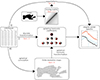 |
Fig. 1. Overview of the methodology presented below. We apply the formalism for discrete angular power spectra in three distinct ways: (i) Exact spherical harmonic coefficients can be computed from the discrete data, without the use of maps. In turn, angular power spectra can be computed from combinations of spherical harmonic coefficients. (ii) The angular power spectra themselves can be computed from the discrete data. This is inefficient for practical computation, but makes it possible to obtain exact expressions for the expected spectra. (iii) The discrete data can be turned into maps, and subsequently into spherical harmonic coefficients by means of a spherical harmonic transform. This can yield the same results as the discrete transformation. |
The methodology presented here, for both the discrete and map-based spectra, is implemented in a publicly available code called Heracles1. This code is used for data processing in the 3 × 2 pt pipeline within the Euclid Science Ground Segment. However, it was designed from the ground up as a modular, adaptable, and user-friendly general-purpose utility that can be used for a multitude of probes and surveys.
2. Angular power spectra
In this section we state the key results and theorems regarding the two-point statistics of arbitrary spherical functions (i.e. functions on the sphere). The crucial point here will be that the concepts of angular power spectra and angular correlation functions are well-defined not only for the particular case of homogeneous random fields, but for any function on the sphere, such as an individual realisation of a random field.
In the following, we always deal with spin-weighted spherical functions, which sometimes have spin weight zero, and we follow the definitions of Boyle (2016). We parametrise the sphere using unit vectors, which we denote  and
and  . A spherical function f has spin weight s if the function value
  transforms under a rotation γ of the coordinate frame in
  as
as
 (1)
(1)
It follows that a spherical function with non-zero spin weight is necessarily complex-valued. Examples of a spin-weighted spherical functions are the global surface temperature on Earth (s = 0), wind speed and direction (s = 1), or the polarisation of the CMB (s = 2).
We generally only consider spherical functions f with spin weight s that have an expansion into spin-weighted spherical harmonics sYlm:
 (2)
(2)
Here and in the following, sums always extend over all admissible values l ≥ |s| and −l ≤ m ≤ l. The coefficients flm of the expansion are obtained by integration against the spherical harmonics,
![Mathematical equation: $$ \begin{aligned} f_{lm} = \int \! f(\hat{u}) \, \bigl [_sY_{lm}(\hat{u})\bigr ]^* \, \mathrm{d}\hat{u}, \end{aligned} $$](/articles/aa/full_html/2025/02/aa52018-24/aa52018-24-eq7.gif) (3)
(3)
where the integral extends over the entire sphere, and an asterisk denotes complex conjugation. For s = 0 (i.e. no spin weight) the expansion is in the classical spherical harmonics Ylm ≡ 0Ylm. In practice, we always have s = 0 or s = 2, but we treat s as an arbitrary integer spin weight as much as possible.
2.1. Two-point statistics
For any pair of spherical functions f and f′ with respective spin weights s and s′, where f = f′ is allowed, we can define the angular correlation Cff′(θ) as the correlation of  and
and  over all points
  on the sphere separated by the angle θ,
 (4)
(4)
Here, if the spin weights s and s′ are non-zero, the angles α and α′, defined in Appendix C, describe a rotation of the respective coordinate frames in  and
and  such that the resulting correlation is frame-independent. It is clear that the definition (4) of the angular correlation function does not require f or f′ to be random fields, or possess any kind of symmetry. If f and f′ are complex-valued, the two-point statistics are not fully characterised by Eq. (4) alone, but also by the correlations between f* and f′, as described in Appendix D.
For any angular correlation function Cff′, we can define an associated angular power spectrum Clff′ as the coefficients of the expansion of Cff′ into the Wigner d functions dss′l (Edmonds 1960),
 (5)
(5)
As usual, the coefficients are obtained by projection against the basis functions,
 (6)
(6)
The definition (5) of the angular power spectrum in terms of the angular correlation function makes once again no reference to random fields or symmetries.
To express the angular power spectrum Clff′ directly in terms of the functions f and f′, we can replace Cff′(θ) in the angular power spectrum (6) by its definition (4),
 (7)
(7)
where the angles α, θ, α′ still depend on  and
and  , but we now have two unrestricted integrals over the sphere. Inserting the spherical harmonic addition theorem
 (8)
(8)
into the integrand in definition (7), the two integrals decouple, and reduce to the spherical harmonic coefficients flm and  given by definition (3). The angular power spectrum of spherical functions f and f′ is hence equivalently defined in terms of their spherical harmonic coefficients,
 (9)
(9)
This expression is sometimes called “the estimator of the angular power spectrum”, for reasons that are given below. However, expression (9) is in fact the true angular power spectrum of the particular spherical functions f and f′ (which, in cosmology, are a particular realisation from a random process), as Clff′ contains exactly the same information as the angular correlation function (4). To fully describe the two-point statistics of complex-valued functions f and f′, we hence require both Clff′ and the pseudo-spectrum Clf*f′ (see Appendix D).
2.2. Homogeneous random fields
The angular correlation function (4) is obtained by averaging a spherical function over all pairs of points at a given angular separation θ. There is an important class of fields where this averaging over direction does not remove information from the two-point statistics. These are the random fields that are invariant under rotations, which we call ‘homogeneous’ on the sphere2.
Under a rotation R of the sphere the coefficients of the spherical harmonic expansion (2) transform as (Boyle 2016)
 (10)
(10)
where Dμml is the Wigner D function. The importance of homogeneous random fields on the sphere is closely related to this transformation: if f is a realisation of such a field, all of its statistical properties are by definition invariant under rotations, and both sides of transformation (10) have the same distribution. The distinction between the random field itself and its realisations is important here: the random field is invariant, but any given realisation that we may observe is a fixed non-random spherical function.
Homogeneity is a powerful tool: for example, consider the product  of modes from the spherical harmonic expansion (2) of a pair of functions f and f′. Under the rotation (10), the product transforms as
 (11)
(11)
If f and f′ are realisations of jointly homogeneous random fields, both sides of transformation (11) must be equal in distribution. Taking the expectation over realisations, denoted ⟨ ⋅ ⟩, we find
 (12)
(12)
Integrating out the rotation R on both sides using the orthogonality of the D functions (Edmonds 1960, Eq. 4.6.1), we recover expression (9), and thus obtain the well-known expectation
 (13)
(13)
where δK is the Kronecker delta symbol. In other words, the modes of homogeneous random fields on the sphere are uncorrelated, unless their modes numbers coincide.
Note that the expectation (13) is sometimes used to define the angular power spectrum ⟨Cl⟩ of random fields, in which case the expression (9) is used as an estimator for ⟨Cl⟩. However, we prefer to think of the sum (9) as the actual, realised, observable angular power spectrum, and ⟨Cl⟩ as its expectation over realisations.
Having obtained the two-point expectation (13) in harmonic space, its equivalent  in real-space can be obtained by computing the spherical harmonic expansion (2) of the product, substituting expectation (13), and using the complex conjugate of the spherical harmonic addition theorem (8):
 (14)
(14)
Factoring out the exponentials, the remaining sum is precisely the expectation of the relation (5) between angular power spectrum and angular correlation function,
 (15)
(15)
and expectation (14) thus yields the expected two-point statistics in real space,
 (16)
(16)
Naturally, the inverse relations (6)–(15) holds in expectation as well,
 (17)
(17)
and is consistent with expectations (16) and (14).
2.3. Mixing matrices
An important special case is a random field f that is the product of a homogeneous random field g and a non-stochastic spherical function w,
 (18)
(18)
We usually call w a weight function, but it is in fact arbitrary, and could in principle encode systematic effects, such as position-dependent multiplicative biases, including higher-order biases with non-zero spin weights (Kitching et al. 2021; Kitching & Deshpande 2022). The functions in the product (18) can each have an associated spin weight; if s, s1, s2 are the respective spin weights of f, g, w, it follows that s = s1 + s2 by the definition of the spin weight (1).
The angular correlation function (4) of f and a second such field f′ can be expressed in terms of g, g′ and w, w′,
![Mathematical equation: $$ \begin{aligned} C^{ff^{\prime }}(\theta )&= \frac{1}{8\pi ^2} {\int \int \limits _{\hat{u} \cdot \hat{u}^{\prime } = \cos \theta }} \Bigl [\mathrm{e}^{\mathrm{i} s_1 \alpha } \, g^*(\hat{u}) \, g^{\prime }(\hat{u}^{\prime }) \, \mathrm{e}^{-\mathrm{i} s_1^{\prime } \alpha ^{\prime }}\Bigr ]\nonumber \\&\qquad \qquad \qquad \times \Bigl [\mathrm{e}^{\mathrm{i} s_2 \alpha } \, w^*(\hat{u}) \, w^{\prime }(\hat{u}^{\prime }) \, \mathrm{e}^{-\mathrm{i} s_2^{\prime } \alpha ^{\prime }}\Bigr ] \, \mathrm{d}\hat{u} \, \mathrm{d}\hat{u}^{\prime }. \end{aligned} $$](/articles/aa/full_html/2025/02/aa52018-24/aa52018-24-eq33.gif) (19)
(19)
To compute the expectation of expression (19), we assume that g and g′ are independent of w and w′. The expectation can then be moved into the integral, and we recover the angular correlation function (16) of g and g′,
 (20)
(20)
We can factor ⟨Cgg′(θ)⟩ out of the integral, which reduces to the angular correlation function (4) of w and w′,
 (21)
(21)
We thus find that the expected angular correlation of products of homogeneous random fields and weight functions is the product of their (expected) angular correlations.
Given expectation (21), we can also compute the expected angular power spectrum using relation (6),
 (22)
(22)
We then expand the angular correlations ⟨Cgg′(θ)⟩ and Cww′(θ) in the integral using relation (5). Since s = s1 + s2 and s′=s1′+s2′, we obtain Gaunt’s integral for the d functions (Edmonds 1960),
 (23)
(23)
where the right-hand side contains the Wigner 3j symbols. The result expresses the expected angular power spectrum ⟨Clff′⟩ in terms of the angular power spectra ⟨Clgg′⟩ and Clww′,
 (24)
(24)
There is hence a convolution theorem for angular power spectra and angular correlation functions, which more generally holds for expansions in Wigner d functions: the product of functions in the real-space expectation (21) corresponds to a convolution in the harmonic-space expectation (24).
In practice, we usually want to keep the weight functions fixed, and compute the expectation ⟨Clff′⟩ as a function of the expected angular power spectrum ⟨Clgg′⟩ of the underlying random fields. In that case, the convolution (24) can be separated into a linear operator containing the sum over l2,
 (25)
(25)
which can subsequently be applied to any given ⟨Cl1gg′⟩,
 (26)
(26)
We call the operator Mww′ the mixing matrix of the weights w, w′ applied to the fields f, f′ and g, g′. This is slightly misleading, since expression (25) is merely a formal matrix with infinitely many rows and columns. However, in practice, it is always truncated to a finite size, and hence indeed a matrix. Note that the mixing matrix (25) not only depends on w and w′, but also on the full set of spin weights.
There is an important, non-trivial consequence of the above derivation: the mixing matrix only maps the expected angular power spectrum of a homogeneous random field to the expected angular power spectrum of its product with another function. The critical step occurs in the expectation (20), which only holds (i) in expectation and (ii) for homogeneous random fields. If either condition is not fulfilled, the mixing matrix formalism breaks down. In particular, it follows that mixing matrices for random fields cannot in general be multiplied: If the function w = w1 w2 is the product of spherical functions w1 and w2, then
 (27)
(27)
except for special cases. The reason is a lack of homogeneity: the random field w2 g that yields the mixing matrix Mw2w2′ is no longer homogeneous, and the product w1 (w2 g) is hence not described by a second mixing matrix application. For example, consider the respective footprint of the northern and southern hemisphere. Individually, both footprints have the same angular correlation function, same angular power spectrum, and same non-vanishing mixing matrix. But since the product of the footprints is identically zero, so is their combined mixing matrix.
3. Discrete observations
Having reviewed the theory of angular power spectra, we now turn our attention towards creating the necessary spherical functions from sets of discrete observations. To this end, we consider two distinct types of observations:
-
Points. The information lies in the distribution of the observed positions themselves, which have no further data attached.
-
Fields. The information comes from the observed values of some underlying spherical function, which is observed in a discrete set of points.
Depending on which kind of data we wish to analyse, we must proceed in slightly different ways.
3.1. Points
We first consider the case where we observe a number of points  , k = 1, 2, …, on the sphere, as well as a set of weights wk3. In the specific case of Euclid, this might be the observed angular positions of galaxies. We can represent the set of observed points as a sum of “point masses” using the Dirac delta function δD,
 (28)
(28)
where the sum extends over the observed points. This turns the discrete observations into a function defined over the entire sphere. The spherical function n has spin weight s = 0 and is a true (weighted) number density, since the integral of the definition (28) over any given area of the sphere produces the contained (weighted) number of observed points.
The spherical harmonic expansion (2) of the observed number density n is readily obtained: inserting the function (28) into the definition (3) of the spherical harmonic coefficients, we can use the defining property of the delta function,
 (29)
(29)
The spherical harmonic coefficients of the number density n are hence simply the weighted, complex-conjugated values of the spherical harmonics in the observed points.
To compute the angular power spectrum (9) of n and a second set of points  with weights w′k′ and associated number density n′, where the two observed sets of points can be one and the same, it suffices to insert the sum (28) of delta functions for n and n′ into definition (7), set the spin weights to zero, and carry out the integration. The result is
 (30)
(30)
where Pl = d00l is the Legendre polynomial, and θkk′ is the angle between  and
and  . This is the exact angular power spectrum for any two sets of points.
3.2. Fields
Next, we consider observations of a set of (complex) function values gk, k = 1, 2, …, which are observed at points  on the sphere, and given weights wk. As in the case of the number density (28), we can construct a spherical function f from the discrete observations using the Dirac delta function δD,
 (31)
(31)
where the sum extends over all observed values. As before, we obtain a function which is defined over the entire sphere. The spin weight s of f is the sum of the respective spin weights s1 and s2 of g and w: if a rotation γ of the sphere in  transforms gk into e−is1γ gk and wk into e−is2γ wk, the function value
  transforms into
  .
.
To compute the spherical harmonic expansion (2) of f, it once again suffices to insert the function (31) into the definition (3) of the spherical harmonic coefficient and use the defining property of the delta function,
 (32)
(32)
The spherical harmonic coefficients are therefore the complex conjugate values of the spin-weighted spherical harmonics in the observed points, multiplied by the observed values and their weights.
To compute the angular power spectrum of f and a second, similarly defined function f′, where both functions can be one and the same, we proceed as above, inserting the sum (31) of delta functions for f and f′ into definition (7) and carrying out the integration. The resulting angular power spectrum for f and f′ is
 (33)
(33)
where the angles αkk′, θkk′, α′kk′ are defined for each pair of points  as in definition (4). This is the exact angular power spectrum given two discrete sets of observed values on the sphere.
The discrete angular power spectrum (33) demonstrates the equivalence between harmonic and real space nicely: it is equivalent to the well-known real-space estimator (Schneider et al. 2002), transformed pair by pair to harmonic space using the transformation (6). In practice, however, the two measurements do contain slightly different information, since we cannot obtain them over all angular scales, which would be required to carry out the transformation mathematically.
3.3. Cross-correlations
Finally, we can consider the case where we wish to obtain the two-point statistics between discrete sets of measured points and measured function values. Following the preceding sections, we can construct spherical functions n and f′ using the sums (28) and (31) of delta functions, respectively. The angular power spectrum is once again obtained by inserting n and f′ into definition (7) and integrating out the delta functions,
 (34)
(34)
where s′ is the spin weight of f′, and the angles θkk′, α′kk′ are defined as above. Naturally, the result (34) is merely the special case of the angular power spectrum (33) when setting f = n, and hence gk ≡ 1 and s = 0.
4. Expectations
We are now able to compute expectations of the angular power spectra (30), (33), and (34) when the observations are random variates, such as the cosmological data observed by Euclid. We once again have to distinguish the cases where we observe points (e.g. galaxy positions) and fields (e.g. cosmic shear). In the first case, we have two-point statistics from observed points, which are generated by point processes on the sphere. In the second case, we have two-point statistics from observed function values, which are generated by random fields.
There is a subtle difference between point processes and random fields beyond the fact that we observe positions for one and function values for the other. It is encoded in what will be called Assumptions 1 and 6 below: to compute an expectation for point processes, we must allow the random positions to vary. This means that we require a priori information about the probability of observing a point anywhere on the sphere. For random fields, we are instead able to compute expectations conditional on the observed positions and weights.
4.1. Point processes, angular clustering
For observations generated by point processes, we compute the expectation of the angular power spectrum (30) for the observed number densities n and n′. To do so, the sum in expression (30) is split into separate sums over the set of true pairs of distinct points (denoted here by k ≢ k′, meaning  and
and  are not the same observed point) and over the set of degenerate pairs of identical points (denoted by k ≡ k′, meaning
  and
and  are the same observed point),
 (35)
(35)
The second sum is sometimes empty, but not always, e.g. when computing an auto-correlation, where n and n′ describe the same observation. Since θkk′ = 0 for k ≡ k′, the second sum contains only Pl(1) = 1, and reduces to the total weight of degenerate pairs of points in n and n′, for which we define
 (36)
(36)
For an auto-correlation, Ann′ is simply the total squared weight. Overall, we thus find that the angular power spectrum (30) can be written as
 (37)
(37)
where the remaining sum contains the two-point statistics from true pairs of distinct points. The term Ann′ is an additive bias from degenerate pairs of identical points, which is often called the ‘noise bias’. However, even though Ann′ is a stochastic quantity over realisations of the point processes, for any given realisation of points, the bias (36) is evidently a known number that we can compute exactly.
We thus subtract Ann′ from both sides of expression (37) and compute the expectation of the bias-subtracted angular power spectrum,
 (38)
(38)
Our goal is to express this expectation in terms of the intrinsic two-point statistics of the point process. The main difficulty lies in the fact that we may not have a complete sample of observations; for example, because we were only able to observe part of the sphere, as happens in any galaxy survey such as Euclid. In addition, there may be complicated observational effects at play, which result in some random points being missed even within the survey footprint. Any systematic removal of points from our sample affects the observed two-point statistics, and must hence be carefully taken into account.
To compute the expectation (38) with missing observations and systematic effects, we set wk = 0 and w′k′ = 0 for all unobserved points  and
and  in the (unknown) complete sample. We can then extend the sum in expression (38) to all points generated by the point process, both observed and unobserved, without changing its value,
 (39)
(39)
Naturally, we have no knowledge about the unobserved points  in the sum, but that will not be a problem for computing the expectation.
Since each realisation of the point process yields a different set of observed points, the weights wk and w′k′ in the expectation (39) are themselves random variables. We can use the law of total expectation to compute the expectation of wk conditional on  , by making
Assumption 1. asmSPSHYP0 There exist functions v and v′ that describe the expected weight conditional on the observed position,
 (40)
(40)
and similarly  .
.
We call v and v′ the (weighted) ‘visibility’ of the respective observation; for unit weights, the value  is a number between 0 and 1 that describes the a priori probability that a point sampled in a given position
  is observed. For general weights, the expectation is also taken over realisations of their values. In practice, estimating the visibility of a galaxy imaging survey is an open problem, and the subject of ongoing research (Johnston et al. 2021; Rodríguez-Monroy et al. 2022).
Using the visibility (40), the expectation (39) no longer depends on the exact set of observed points,
 (41)
(41)
In fact, the expectation of the sum in expression (41) depends solely on the pairs of points  in a given realisation. We can hence make
Assumption 2. asmSPSHYP1 All observed pairs of points have the same a priori distribution.
This is a weak assumption, since it is difficult to imagine how any specific pair of points in a realisation might be a priori distinguishable from the rest.
Under Assumption 2, all terms in the sum in expression (41) have the same expectation. If N and N′ are the respective total number of points for each point process, there are NN′ pairs of points4, and hence terms in the sum. Introducing functions  and
and  with
with
 (42)
(42)
and similarly  , the expectation (41) is
 (43)
(43)
where  is a pair of random points, and θ is the angular separation between them. The functions
  and
and  can be understood as the position-dependent mean density of the observed points, taking the visibility into account. This has the conceptual advantage that we never have to define the exact sample of points to which N and
  refer, which would be difficult for Euclid with its complicated coverage from different ground-based surveys.
The remaining expectation on the right-hand side of expression (43) contains two random effects: one is the angular distribution of points, and the other is the random realisation of the mean densities. Here, we are only interested in the former, and we therefore make
Assumption 3. asmSPSHYP2 The expected angular power spectrum is conditional on the observed densities of points.
To see why the expectation over realisations with varying density is not very interesting, one can imagine a point process where the distribution of points is smoother or clumpier depending on the realised density. In that case, the expected two-point statistics over all densities can be arbitrarily different from the expectation conditional on the observed density, and we can extract essentially no information from our measurement. We hence want to compute an expectation that is, in some sense, close to our observation, except for the angular distribution of the points. This also agrees with intuition, since the (conditional) expectation of the observed density (28) over realisations of positions is then equal to the mean density (42),
 (44)
(44)
However, our assumption comes with two important caveats: firstly, for galaxy clustering, the number of galaxies (as well as their weights, if given) will depend to some degree on the underlying realisation of the universe, and we are hence assuming that this correlation can be neglected. Secondly, in practice, we have no a priori knowledge about the mean density  , and we must hence estimate it from the observations themselves. We check the impact of the latter point in Sect. 6.
Using Assumption 3, only the expectation over positions remains in expression (43), which is a double integral over the sphere,
 (45)
(45)
with  the a priori probability of the point process to generate a pair of points in
  . In the general case, this integral must be evaluated explicitly. But for the point processes in which we are interested here, we can make
Assumption 4. asmSPSHYP3 The point processes are homogeneous on the sphere, i.e. their distribution is unchanged under rotations of the sphere.
For galaxy clustering, this assumption is usually granted by the “cosmological principle”.
Under Assumption 4, the joint probability density  in the integral (45) depends only on the angular distance θ between the pair of points
  and
and  . It can be written as (Landy & Szalay 1993; Peebles 1973)
 (46)
(46)
where 𝔴 is the expected angular correlation function of density fluctuations in the observed point processes, which describes the clustering of points5.
Inserting the integral (45) and joint probability density (46) into expectation (43), we find that only  and
and  depend explicitly on the positions
  and
and  , while everything else depends on the angular separation θ alone,
![Mathematical equation: $$ \begin{aligned} \langle {C_l^{nn^{\prime }} - A^{nn^{\prime }}}\rangle = \frac{1}{4\pi } \int \int \! \bar{n}(\hat{u}) \, \bar{n}^{\prime }(\hat{u}^{\prime }) \, \bigl [1 + \mathfrak{w} (\theta )\bigr ] \, P_l(\cos \theta ) \, \mathrm{d}\hat{u} \, \mathrm{d}\hat{u}^{\prime }. \end{aligned} $$](/articles/aa/full_html/2025/02/aa52018-24/aa52018-24-eq99.gif) (47)
(47)
Writing the double integral over the sphere in terms of the angular separation θ recovers precisely the definition (4) of the angular correlation function  ,
,
![Mathematical equation: $$ \begin{aligned} \langle {C_l^{nn^{\prime }} - A^{nn^{\prime }}}\rangle = 2\pi \int _{0}^{\pi } \! C^{\bar{n}\bar{n}^{\prime }}(\theta ) \, \bigl [1 + \mathfrak{w} (\theta )\bigr ] \, P_l(\cos \theta ) \sin (\theta ) \, \mathrm{d}\theta . \end{aligned} $$](/articles/aa/full_html/2025/02/aa52018-24/aa52018-24-eq101.gif) (48)
(48)
Integrating the two terms of 1 + 𝔴(θ) separately, the former is the transformation (6) from  to
to  , while the latter is the convolution (22) of
  and 𝔴(θ), which we can write in the form of a mixing matrix product (26). Overall, we can hence write the expectation (48) as
 (49)
(49)
where  is the mixing matrix (25) due to the mean density functions
  and
and  , and 𝔴l is the angular power spectrum of the point processes, obtained from the intrinsic angular correlation function 𝔴 using relation (6).
We hence find that the expectation (49) contains the desired intrinsic two-point statistics of the point processes, in the form of 𝔴l. However, the signal is doubly contaminated when the mean densities  and
and  contain systematic variations, by both the angular power spectrum
  and by the associated mixing matrix
  . To remove these contaminations, we can directly manipulate expression (49) until it yields an estimator for 𝔴l. While this approach is somewhat unusual in harmonic space, we show in Appendix B that it recovers well-known results from real space, such as the estimator of Landy & Szalay (1993).
In what follows, we focus instead on the more traditional approach for isolating the signal 𝔴l in the expectation (49). We directly construct spherical functions δ and δ′ for the number density contrast of the observed points,
 (50)
(50)
and equivalently for  , where
  denotes the total mean density over the sphere. Note that we divide here by a constant, and not by the function
  ; for the alternative case (see Appendix B). The density contrast (50) is hence a linear combination of the spherical functions n and
  , and it follows that the angular power spectrum of δ and δ′ is
 (51)
(51)
We therefore find that measuring the angular power spectrum of the number density contrast (50) yields a result that is equivalent to the partial-sky harmonic-space Landy–Szalay estimator (B.4). The expectation ⟨Clδδ′⟩ of the angular power spectrum (51) is readily computed using expressions (42), (44), and (49),
 (52)
(52)
where Mvv′ is the mixing matrix for the visibilities v and v′, and  is the rescaled additive bias.
4.2. Random fields, cosmic shear
The second case of interest is where we observe values gk which are the variates of an underlying random field, and use them to construct a spherical function f using definition (31). If there is a spherical function g such that the observations are the function values  of g in the observed points, we can use the defining property of the delta function to factor
  out of the sum in definition (31),
 (53)
(53)
For the remaining sum, we introduce a spherical function w, which we call the ‘weight function’ of the random field,
 (54)
(54)
We can therefore write  , and understand our constructed function f as the product of the function g under observation and a weight function w that encodes where and how well g has been observed. While the visibility (40) of a point process is, firstly, an expectation and, secondly, usually a relatively smooth function over the sphere, the weight function (54) of a random field consists of the given weights wk in the observed positions
  .
.
If the function g is the realisation of a random field, we want to use the mixing matrix formalism (26) to compute the expectation of the angular power spectrum (33) of f and a second such function f′ with  . To this end, we firstly require
Assumption 5. asmSPSHYP7 The functions g and g′ are realisations of jointly homogeneous random fields.
In the case of cosmic shear, this is once again a reasonable assumption by the cosmological principle. To apply the mixing matrix formalism, we further require
Assumption 6. asmSPSHYP4 The distribution of observed values gk is conditional on the observed positions  and weights wk.
For cosmic shear, this assumption implies two approximations. Firstly, it ignores that the positions of galaxies are slightly correlated with their shears (source–lens clustering, Linke et al. 2024), since both positions and shears are ultimately connected to the large-scale structure of the universe. Secondly, the weights and values of shear observations are generally also slightly correlated, since more extreme galaxy shapes are harder to measure accurately, and thus given lower weights.
Under Assumptions 5 and 6, only the functions g and g′ are considered realisations of (homogeneous) random fields when computing the expectation of the angular power spectrum (33) for f = g w and f′=g′ w′, while w and w′ are considered fixed functions. We can hence use the mixing matrix formalism (26) to obtain the expected angular power spectrum of f and f′,
 (55)
(55)
where the mixing matrix is computed for the weight functions w and w′ of point masses following definition (54).
The situation is slightly more complicated if we observe the field g only indirectly via some intermediary observable. For cosmic shear, that observable is the galaxy ellipticity ϵk, which probes the cosmic shear field through the effect of weak gravitational lensing on the intrinsic galaxy shapes (e.g. Bartelmann & Schneider 2001),
 (56)
(56)
where ϵki is the intrinsic galaxy ellipticity that would have been observed without gravitational lensing. We say that the ellipticity ϵk traces the cosmic shear field g, because the conditional expectation of ϵk for a fixed value gk and random orientations of the galaxy is (Seitz & Schneider 1997)
 (57)
(57)
However, even though the observed ellipticity is an unbiased estimate of the cosmic shear field, the intrinsic variability of galaxy shapes leads to an increase in variance compared to the pure cosmic shear signal,
 (58)
(58)
The second term in expectation (58) is an additional variance commonly called shape noise, and we see that the effect depends on both the variance of the intrinsic galaxy ellipticity and the one-point statistics of the cosmic shear field. In practice, there is a further contribution to shape noise due to the variance from imperfect shape measurement.
To understand the impact of noise on the expected angular power spectrum of a random field g, we make
Assumption 7. asmSPSHYP5 Observed values of the random field g have independent noise contributions.
Taken in isolation, this is not a good approximation for the shape noise of cosmic shear, since galaxies have intrinsic alignments (Joachimi et al. 2015; Kiessling et al. 2015; Kirk et al. 2015; Troxel & Ishak 2015). However, intrinsic alignments are generally absorbed into the theoretical prediction of the cosmic shear signal, so that our assumption is effectively a statement about our capability to model this effect.
Under Assumption 7, the expectation (55) of the angular power spectrum does not change its signal content, but picks up an additional variance term,
 (59)
(59)
where Aff′ is the additive bias due to the noise variance σkk′2 from degenerate pairs of identical objects (denoted as before by k ≡ k′)6,
 (60)
(60)
where s and s′ are the spin weights of f and f′, respectively, as before. For random fields, the additive bias Aff′ is therefore a true noise bias, in the sense that it is the expectation of a stochastic noise contribution, unlike the additive bias Ann′ of the point process, which is a known number for each realisation.
For cosmic shear, we do not know, a priori, the additional variance σkk′2 due to shape noise for each observed value gk or g′k′. In that situation, we can construct an estimate 𝒜ff′ of the additive bias from the variance of the noisy observations (Nicola et al. 2021),
 (61)
(61)
By expectation (58), this is a biased estimator for a non-vanishing Aff, since it contains not only the variance due to shape noise, but the sum of intrinsic and noise variance,
 (62)
(62)
where the expected zero-lag angular correlation ⟨Cgg′(0)⟩ is the intrinsic variance of the random fields g and g′. Subtracting 𝒜ff′ from the measured angular power spectrum Clff′ and taking the expectation using expressions (59) and (62), we obtain
 (63)
(63)
Noting that the two-point statistics of g and g′ enter both terms on the right-hand side of the expectation, we use relation (5) and the properties of the Wigner d function to replace ⟨Cgg′(0)⟩ by a sum over the expected angular power spectrum,
 (64)
(64)
with s1 and s1′ the respective spin weights of g and g′, as above. The expectation (63) is therefore equivalent to
 (65)
(65)
where we have introduced the reduced mixing matrix
 (66)
(66)
In the expectation (65), the bias introduced by 𝒜ff′ is thus completely absorbed into ℳll1ww′.
As it turns out, the reduced mixing matrix has a much simpler interpretation than the definition (66) suggests. Consider the angular power spectrum (33) for the pair of weight functions w and w′ with respective spin weights s2 and s2′. Following expression (35), we split Clww′ into contributions from true pairs of distinct points (k ≢ k′) and degenerate pairs of identical points (k ≡ k′), so that we may define the known additive bias Aww′ for the weight functions w and w′,
 (67)
(67)
Since s = s1 + s2 and s′=s1′+s2, we can substitute Aww′ for the sum in expression (66),
 (68)
(68)
Furthermore, we can substitute the Kronecker symbols by an identity for the Wigner 3j symbols,
 (69)
(69)
Using the fact that Aww′ vanishes unless s2 = s2′, an equivalent way to write expression (68) is therefore
 (70)
(70)
Comparing the result to the definition (25) of the mixing matrix, we indeed obtain a straightforward interpretation of the reduced mixing matrix,
 (71)
(71)
In other words, the reduced mixing matrix is the mixing matrix of the angular power spectrum Clww′ with its additive bias Aww′ subtracted.
To summarise, we obtain the following four key results. For noisy observations where the additive bias to the angular power spectrum is not known, which is the case for cosmic shear, we can construct the estimate (61) using the variance of the noisy observations. Subtracting the estimated additive bias from the measured angular power spectrum leads to a biased expectation (63) with respect to the mixing matrix formalism, since the estimate contains not only the additional variance due to noise, but also the intrinsic variance of the fields. However, we can return the expectation (65) to standard form by introducing a reduced mixing matrix, which implicitly removes the intrinsic variance of the random fields from the expected angular power spectrum. Finally, the reduced mixing matrix (71) is simply the mixing matrix with the additive bias of the weight functions, which is a known number, subtracted.
The nature of this correction becomes clear in real space. The unknown noise variance σ2 is a delta-like contribution to the expected angular correlation function of the random fields,
 (72)
(72)
Subtracting the additive bias from the angular power spectrum is equivalent to subtracting the variance, which is the zero-lag correlation, from the angular correlation function. There is hence a correspondence
 (73)
(73)
for the random fields, and
 (74)
(74)
for the weight functions. By expectation (21), the real-space equivalent of the reduced mixing matrix expectation (65) is hence
![Mathematical equation: $$ \begin{aligned}&\Big \langle {C^{ff^{\prime }}(\theta ) - C^{ff^{\prime }}(0) \, \delta ^\mathrm{D}(\cos \theta - \cos 0)}\Big \rangle \nonumber \\&\qquad = \Bigl [\langle {C^{gg^{\prime }}(\theta )}\langle + \sigma ^2 \, \delta ^\mathrm{D}(\cos \theta - \cos 0)\Bigr ] \nonumber \\&\qquad \qquad \times \Bigl [C^{ww^{\prime }}(\theta ) - C^{ww^{\prime }}(0) \, \delta ^\mathrm{D}(\cos \theta - \cos 0)\Bigr ], \end{aligned} $$](/articles/aa/full_html/2025/02/aa52018-24/aa52018-24-eq149.gif) (75)
(75)
where we can evaluate the right-hand side for all θ ≥ 0 without knowing the value of σ2.
4.3. Cross-correlations, galaxy–galaxy lensing
The final case of interest is the cross-correlation of points  generated by a point process, and observed values
  from the realisation g of a random field. The two observations define the spherical functions n and f′ as above.
For the expectation of the angular power spectrum (34) of n and f′, we again fundamentally rely on Assumption 6: the distribution of observed values g′k′ is conditional on the observed points  and weights w′k′, which are held fixed. We assume that this remains true even when correlating positions and values from a single observation, in which case the observed positions are both random variates (within n) and fixed (within w′ and hence f′). For galaxy–galaxy lensing, the approximation performs worse than for cosmic shear; this is seen in Sect. 6. As in the case of intrinsic alignments, the assumption is therefore effectively a statement about our ability to model the effect of source–lens clustering in the theory part of the expectation.
To treat the point process in the expectation of the angular power spectrum (34), we proceed as before. We extend the sum over k to all points using the visibility (40), and replace wk by  under Assumption 1,
 (76)
(76)
While Assumption 2 considers pairs of points, here we only have a single set, and hence make
Assumption 8. asmSPSHYP6 All random points in the cross-correlation have the same a priori distribution.
As in the case of pairs of points, this seems a weak assumption, since it is difficult to imagine how individual points might be a priori distinguishable from each other.
Under Assumption 8, the sum over k in expectation (76) reduces to N identically distributed terms. Using definition (42), we can replace the product of N and visibility v by the mean number density  . Using the definition (54) of the weight function w′, we may also replace the remaining sum over k′ by an integral over
  ,
,
 (77)
(77)
where the angles θ and α′ now describe the relative orientation between the random point  and
and  .
.
Using Assumption 6, we can factor the weight  out of the integral in expectation (77). Furthermore, using Assumption 3, the expectation is conditional on the mean number density
  , and only the position
  in
in  is random. The remaining expectation in Eq. (77) therefore reduces to the random point
  and the random field g′. It can be computed in two steps using the law of total expectation. Using the angular correlation (16), the expectation of a homogeneous (by Assumption 5) random field g′ conditional on
  is
is
 (78)
(78)
where γ is the expected angular cross-correlation function7. For galaxy–galaxy lensing, the expected correlation is more commonly written in terms of a tangential component γt and cross-component γ× as γ(θ) = γt(θ)+i γ×(θ).
Combining expectations (78) and (77), it remains to compute the expectation over random positions  . Under Assumption 4, the point process is homogeneous, and hence
 (79)
(79)
As before, the double integral recovers the definition (4) of the angular correlation function for  and w′,
 (80)
(80)
which in turn is the convolution (22) of  and γ that yields the mixing matrix (26),
 (81)
(81)
where γl is the angular power spectrum associated with the angular cross-correlation function γ.
Overall, we therefore obtain the intuitively clear result that the expected angular power spectrum is given by the intrinsic spectrum γl for point process and random field, modulated by a mixing matrix coming from the mean number density  (due to the point process) and weight function w′ (due to the random field).
In the case of two point processes, it was advantageous to correlate the density contrast δ instead of the number density n. Since the density contrast (50) is linear in n, the angular power spectrum of δ and f′ is
 (82)
(82)
The expectation ⟨Clδf′⟩ then follows immediately from the definition (42) of the mean density and expectation (81),
 (83)
(83)
where the second equality assumes that the expectation of f′ vanishes.
Whether to correlate n or δ is a well-known question for real-space estimators of galaxy–galaxy lensing (Joachimi et al. 2021). Formally, we can construct a direct estimator of the signal from either the number density n using expectation (81),
 (84)
(84)
or from the density contrast δ using expectation (83) and the definition (42) of the mean density,
 (85)
(85)
In real space, the mean number density  corresponds to an equivalent distribution of uniform random points (‘randoms’); the inverse mixing matrix in both
  and
and  thus corresponds to a normalisation by weighted pairs of randoms and the observed positions of the field. The difference between
  and
and  is the second term in the estimator (85), which corresponds to correlations between randoms and field values. It was shown by Singh et al. (2017) that the estimator (85) has lower variance relative to the estimator (84), particularly on large scales, because it suppresses covariance terms that couple with the survey mask. This suppression also increases the accuracy of covariance estimation via resampling techniques, as these modify the effective survey window in the subsampling compared to the original survey. Moreover, the subtraction of correlations around random points can subtract residual additive systematics in the signal. As in the case of angular clustering, we therefore generally prefer the density contrast δ instead of the number density n to measure cross-correlations.
5. Finite resolution maps
The preceding sections demonstrate how we can obtain angular power spectra from discrete observations, and how we can relate their expectations to the intrinsic two-point statistics of the observed point processes or random fields. We now turn to the practical task of computing the angular power spectra. Retracing our steps, we find that this can be done in one of two ways:
-
(i)
Compute Clnn′, Clff′, and Clnf′ directly using their respective expressions (30), (33), and (34).
-
(ii)
Compute nlm and flm from their analytical expansions (29) and (32), then compute the angular power spectra (9) from the spherical harmonic coefficients.
If N is the number of observations, and lmax is the highest angular mode number of interest, then the former method has a runtime complexity of O(N2lmax), i.e. quadratic in the number of observations, which is the same as for real-space estimators. The complexity of the latter method, however, is O(Nlmax2), and it is hence favourable when lmax ≪ N. We therefore generally want to obtain angular power spectra Cl from their constituent coefficients alm.
The alm computed from the sums (29) and (32) potentially still contain more information than we need: if the observed points are sufficiently dense, they probe scales beyond our desired scale of lmax. We can then reduce the computational complexity further by introducing a spatial binning of the points – or, in other words, by making a map.
Map-making consists of two separate but related parts. The first is sampling, so that spherical functions are represented by their values in a finite set of basis points on the sphere. The number and locations of the basis points are chosen such that it is possible to accurately recover angular modes up to some given lmax from the spherical harmonic expansion (2). Several sampling schemes for that purpose have been proposed; commonly used in astronomy are, e.g. the scheme of Driscoll & Healy (1994), schemes with exact spherical harmonic transforms for band-limited functions (Huffenberger & Wandelt 2010; McEwen & Wiaux 2011), and HEALPix (Górski et al. 2005).
Sampling a random set of point masses, such as the spherical functions (28) and (31) we construct from our discrete observations, with a fixed set of basis points will result in a map that is almost surely zero everywhere. The second part of map-making is hence the collection of function values (i.e. observed points) over a finite region around each sampling point. This is achieved using spherical convolution, which we define below. The area over which observations are collected is, at least in principle, entirely independent of the sampling scheme. Naturally, we want every observation to be counted, in which case this area must be large enough to cover the spaces between sampling points. On the other hand, the area should also not be much larger than necessary, or we needlessly degrade the angular power spectra that we wish to measure. In practice, there is hence always a close match between the convolution and the sampling scheme.
5.1. Spherical convolution
Convolution is a mathematical operation that produces a new function F from a given function f and convolution kernel K. The value of the convolution in a point is obtained by making this point the origin of a local copy of K and computing the integral of f weighted by that kernel. Convolution is therefore not a local operation. And since spin-weighted spherical functions are always defined relative to a local coordinate frame (Boyle 2016), it follows that convolution on the sphere has to explicitly take this non-local nature into account.
As an illustrative example, consider the following situation, where the dot marks the centre of a small, essentially flat patch of the sphere, and the arrows indicate the complex argument of a local spin-weighted function of constant magnitude:
Intuitively, the sum of the function values should be zero. Not accounting for coordinate frame effects, this is indeed the case if the dot is near the equator. But if the dot marks the north pole, all arrows point north, and naive summation produces an incorrect result.
For a spherical convolution that treats non-zero spin weights in the correct manner, we define the convolution F of a spherical function f and a symmetric convolution kernel K as
 (86)
(86)
where the angles θ, α, α′ are the separation and relative orientation of  and
and  as in the spherical harmonic addition theorem (8). Here, s is the spin weight of the convolved function f, and S is the spin weight of the convolution F. We can choose S freely: under a rotation of γ in
  , the angle α in the convolution (86) transforms as α ↦ α − γ, so that F indeed picks up the phase factor e−iSγ of a function with spin weight S. Overall, the convolution (86) is equivalent to the directional spin-weighted spherical convolution of McEwen et al. (2015) with a symmetric kernel, and reduces to the usual spherical convolution of scalar functions when the spin weight is zero (e.g. Wandelt & Górski 2001).
Most importantly, the definition (86) of spherical convolution yields a useful convolution theorem for spherical harmonic expansions. The convolution kernel K is a function of separation, similar to an angular correlation function, so that we can apply the expansion (5) into Wigner d functions,
 (87)
(87)
where the coefficients Kl of the expansion are given by (6),
 (88)
(88)
Inserting the expansion (87) into definition (86) and substituting the addition theorem (8) yields the integral (3) for the coefficients flm in the spherical harmonic expansion (2) of f. We thus obtain the desired spherical harmonic convolution theorem,
 (89)
(89)
where the coefficients Flm of the convolution F are the product of the coefficients Kl of the convolution kernel K and the coefficients flm of the convolved function f.
Carrying out the convolution (86) requires computing the phase factors eiSα and e−isα′ at each point, which can often be done efficiently (see Appendix C). However, if the support of the convolution kernel K is sufficiently small, the local geometry is close to flat, and α ≈ α′. In that case, the phase factors reduce to unity if we choose a convolution with S = s that does not change the spin weight of the function.
It remains to find a tractable convolution kernel K. For a function f with s = 0, the natural choice is a spherical disc of some chosen angular size β > 0. However, for s ≠ 0, the same kernel does not produce analytically tractable coefficients (88) for the convolution theorem. We hence propose a modified convolution kernel that works for any spin weight S = s ≥ 0, and reduces to a spherical disc if s = 0,
![Mathematical equation: $$ \begin{aligned} K(\theta ) = \left\{ \begin{array}{ll} \bigl [\cos \tfrac{\theta }{2}\bigr ]^{2s}&\mathrm{if}\; \theta \le \beta , \\ 0&\mathrm{otherwise}, \end{array}\right. \end{aligned} $$](/articles/aa/full_html/2025/02/aa52018-24/aa52018-24-eq191.gif) (90)
(90)
where β is the angular size (i.e. radius) of the kernel. The effective area of the convolution kernel is8
![Mathematical equation: $$ \begin{aligned} \Omega _K = 2\pi \int _{0}^{\pi } \! K(\theta ) \sin (\theta ) \, \mathrm{d} \theta = 4\pi \, \frac{1 - \bigl [\cos \frac{\beta }{2}\bigr ]^{2s+2}}{s+1}\cdot \end{aligned} $$](/articles/aa/full_html/2025/02/aa52018-24/aa52018-24-eq192.gif) (91)
(91)
The choice of kernel (90) is firstly motivated by the fact that there is a known expression for its coefficients (88)9,
![Mathematical equation: $$ \begin{aligned} K_l = {\left\{ \begin{array}{ll}\frac{4\pi \, \bigl [\sin \tfrac{\beta }{2}\bigr ] \, \bigl [\cos \tfrac{\beta }{2}\bigr ]^{2s+1} \, d^l_{ss+1}(\beta )}{\sqrt{l \, (l+1) - s \, (s+1)}}&\mathrm{if}\;l > s, \\ [3pt] 4\pi \, \frac{1 - \bigl [\cos \frac{\beta }{2}\bigr ]^{4s+2}}{2s+1}&\mathrm{if}\;l = s.\end{array}\right.} \end{aligned} $$](/articles/aa/full_html/2025/02/aa52018-24/aa52018-24-eq193.gif) (92)
(92)
Secondly, for small kernel sizes β ≲ 1°, the convolution kernel (90) is essentially a flat spherical disc even when the spin weight is s = 2 (Fig. 2), in which case the coefficients (92) for s = 0 and s = 2 become essentially the same (Fig. 3). This makes the specific kernel (90) a good practical choice for maps when the resolution is below the degree-scale.
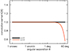 |
Fig. 2. Convolution kernel (90) with no cut-off for spin weight s = 0 (black) and spin weight s = 2 (red). For sufficiently small angles the convolution kernel becomes indistinguishable from a flat spherical disc even in the spin-weighted case. |
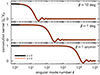 |
Fig. 3. Normalised coefficients of the convolution kernel (90) for spin weights s = 0 (black), s = 2 (red), and kernel sizes β = 10° (top), β = 1° (middle), β = 1 arcmin (bottom). There is excellent agreement between the coefficients for s = 2 and s = 0, except in the case of a large kernel (β = 10°) at large angular scales (l < 10). |
In summary, the convolution (86) means that we can create finite resolution maps of the point-mass like number density (28) or field (31) by picking a sampling scheme and for each grid point summing each observed point with the weight K(θ) given by the convolution kernel K, omitting the phase factors in the convolution (86) if the resolution allows it. For a convolution kernel such as (90) with small angular size β ≪ π, an alternative method is to reverse the order of operations, and find all grid points closer than β for each observed point. This can result in vast performance improvements, particularly if the grid points can be queried efficiently, e.g. when using Cartesian or HEALPix grids.
Once maps are created, it suffices to compute their spherical harmonic coefficients Flm, and reconstruct the coefficients flm of the spherical function from the convolution theorem (89),
 (93)
(93)
Naturally, this is only possible when Kl ≠ 0, which limits the angular mode numbers l that can be recovered for a given convolution kernel. However, if the deconvolution (93) is possible for all numbers l ≤ lmax, we are readily able to compute the angular power spectrum (9) of f and f′ from the finite-resolution maps F and F′. In cases where the deconvolution is impossible or undesirable, we can instead use the convolution theorem (89) to model the effect of the convolution on the expected angular power spectra. In practice, this can be done at no computational cost, by absorbing the convolution kernel into the mixing matrix (26).
5.2. HEALPix pseudo-convolution
Even for small kernels, the radius search required by the spherical convolution comes at a non-negligible computational cost. Given the number of galaxies observed by Euclid, this cost quickly becomes prohibitive, unless faster, specialised algorithms can be found. However, when using the HEALPix grid for sampling, we can alternatively follow the standard procedure of simply summing the points in each HEALPix pixel. But even though all HEALPix pixels have the same area, this operation is not a true spherical convolution, due to the slightly varying pixel shapes (Górski et al. 2005). Nevertheless, summation over HEALPix pixels does obey the convolution theorem (89) approximately, and the normalised coefficients ΩK−1Kl are known as the HEALPix pixel window function (Fig. 4). As it turns out, this pseudo-convolution can be adequate for Euclid analysis, which we demonstrate in Sect. 6.
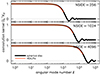 |
Fig. 4. HEALPix pixel window function (red) for resolution parameters NSIDE = 256 (top), NSIDE = 1024 (middle), NSIDE = 4096 (bottom). Also shown is the convolution kernel of a spherical disc with the same pixel area (black). The HEALPix pixel window function is only provided up to l = 4 NSIDE, where it starts to fall below the kernel of the spherical disc. |
There is, however, one fundamental difference between a true spherical convolution and HEALPix pseudo-convolution. According to the convolution theorem (89), the convolution kernel Kl is imprinted on all spherical harmonic coefficients of a map, and consequently on the angular power spectrum (9),
 (94)
(94)
In particular, it follows that the convolution kernel should also affect additive bias terms such as Ann′ in the spectrum (37) of point processes, or Aff′ in the expected spectrum (59) of random fields. These bias terms will therefore no longer be constant after a true convolution. This is not the case for the HEALPix pseudo-convolution (Fig. 5), since the non-overlapping HEALPix pixels cannot imprint structure, such as the convolution kernel, below the pixel scale. In fact, a similar effect occurs when sampling a true convolution so sparsely that the convolution kernel areas no longer overlap.
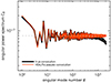 |
Fig. 5. Angular power spectrum of 1 000 000 uniform random points, computed using the HEALPix pseudo-convolution (red) and a true convolution with spherical discs of the same area (black). Both results agree with their respective expectation (dashed). The convolution kernel is only imprinted on the true convolution. |
There is a practical consequence of this difference between true convolution and HEALPix pseudo-convolution. For a map created by true convolution, the deconvolution (93) turns an additive bias term in the angular power spectrum back into a constant. For a HEALPix map, the same deconvolution of the pixel window function turns an additive bias A into an l-dependent bias A/Kl2. When comparing HEALPix spectra and their expectations, the additive bias must therefore either be subtracted from the measured spectra before deconvolution of the pixel window function, or the correct l-dependent bias must be used, e.g. in expectations (49), (52), and (59).
5.3. Maps
We can now define the maps we make. For simplicity, we always call one value of a finite map a pixel with area ΩK, with the understanding that this may refer either to an actual HEALPix pixel or to the kernel of a true convolution.
The convolution of the number density n with definition (28) is the map N of number counts in each pixel. The convolution of  is the map
  of mean number counts; we write it as
  using the mean number of points per pixel
  and a map V that is the convolution of v divided by ΩK. We call V the ‘visibility map’, since it is the pixel-averaged equivalent of the visibility v, with pixel values between 0 and 1. Since the convolution (86) is a linear operation, the expectation (44) translates from the number densities to the number count maps,
  .
.
To isolate the clustering signal in the number count map N, we define a map Δ for the density contrast (50),
 (95)
(95)
It is clear that Δ is the convolution of δ, but divided by the pixel area, so that the numerical values of Δ have the correct, intuitive scale where −1 means “empty space”. Deconvolution of Δ must therefore be carried out with the normalised convolution kernel ΩK−1 Kl.
For a field f (e.g. cosmic shear), we compute the map F by summing the weighted field values wk fk in each pixel, and dividing the result by a constant mean pixel weight  . Specifically, we choose
  to be the mean weight divided by the mean visibility, as computed from the maps, which makes
  relatively insensitive to the survey footprint and systematics. The map F is hence the convolution of the function f with definition (31), divided by
  to remove explicit dependencies on pixel area and overall weight factors. Similarly, we compute the weight map W as the total weight in each pixel, i.e. the convolution of w with definition (54), divided by
  .
.
Since  contains a factor of the pixel area, deconvolution of F and W is carried out with the normalised convolution kernel ΩK−1 Kl. Furthermore, since both F and W are scaled identically, the resulting mixing matrix automatically applies the correct factors of
  to the expected angular power spectra. However, we do need to account for the scaling by
  when computing any additive bias terms.
In particular, we do not average the field values in each pixel by dividing the map F by the map W. For Euclid, the resolution of our maps is such that about half of all observed pixels contain fewer than two observed values. Using a weighted average would simply divide out the given weights in these pixels, resulting in an unweighted cosmic shear map (see, e.g. Hikage et al. 2011, 2019; Nicola et al. 2021). This is clear when looking at the spherical functions f and w with definitions (31) and (54), respectively: dividing f by w where both are non-zero is equivalent to using unit weights in f.
6. Validation
In the preceding sections, we derive the overall theory of angular power spectra from discrete sets of observations, their expectations, and ways to efficiently compute spectra from maps. We now turn to the validation of our findings. One part of this are the explicit assumptions that we have made throughout; these represent specific scientific questions that are partially the subject of active research in their own right, and we do not investigate their validity here.
In what follows, we validate our specific implementation of the methodology described above. This is a publicly available code called Heracles1, developed within the Euclid Science Ground Segment. It contains routines for catalogue reading, map-making, spherical harmonic transforms, angular power spectra, and mixing matrices. The code can be used as a Python library, e.g. for data exploration in a notebook interface, or via a standalone command-line interface, e.g. for batch data processing. In particular, the code also contains an implementation of the discrete angular power spectrum methodology, which is based on fast, non-uniform computation of spherical harmonics (Reinecke et al. 2023) as implemented in the ducc package10.
To validate the performance of Heracles, we carry out the following series of tests:
-
(i)
We estimate the mean density of galaxies from the visible sky fraction in the various Euclid data releases,
-
(ii)
we test if the phase factors in the spherical convolution can be neglected for map-based spectra,
-
(iii)
we assess the overall accuracy of our measurements, and
-
(iv)
we apply the methodology in a data processing setting that mimics the first Euclid data release.
Where simulations are created, we generally employ the same flat ΛCDM cosmology as Euclid’s Flagship simulation (Euclid Collaboration: Castander et al. 2025), with parameter values Ωm = 0.319, Ωb = 0.049, As = 2.1 × 10⁻⁹, ns = 0.96, and h = 0.67.
6.1. Mean density estimation
Constructing the density contrast (50) requires knowledge of the mean density of galaxies over the entire sky, which we must estimate from the visible sky fraction. If our estimate is inaccurate, we bias the angular power spectrum Clδδ′ in a non-trivial manner with respect to the expectation (52). The problem in estimating the mean density accurately is that the visible part of the sky might be particularly over- or underdense compared to the true mean. The probability of this depends on the area of the observed sky, as well as the typical size of large-scale density fluctuations, and hence the clustering of points. This problem is closely related to the integral constraint for real-space estimators.
To test the impact on Euclid observations, we generate 10 000 lognormal realisations of a galaxy distribution with a linear galaxy bias (Tessore et al. 2023). To account for the redshift evolution of galaxy clustering, we test redshifts z = 0.5, 1.0, 2.0, using a redshift-dependent bias that was fitted to the Euclid Flagship simulation (Euclid Collaboration: Lepori et al. 2022). Since the error in the mean density is a function of visible sky fraction, we further use a representative footprint (Euclid Collaboration: Scaramella et al. 2022) for each of the three Euclid data releases DR1 (1 year, 6% sky coverage), DR2 (3 years, 18% sky coverage), and DR3 (6 years, 36% sky coverage). The results show that the expected relative error in the mean density is at the per mille level for all data releases and redshifts, with a scatter that stays below the per cent level for DR2 and beyond (Fig. 6).
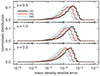 |
Fig. 6. Simulated distribution of the relative error when estimating the mean density |

6.2. Phase factors
To test whether or not we can neglect the phase factors in the convolution (86), we need to quantify their impact on maps at the required resolution for Euclid. Consider a fixed pixel located at a position  . By neglecting the phase factors, the convolution (86) is approximated as
 (96)
(96)
To cancel the phase factors, the approximation effectively applies a position-dependent multiplicative bias e−i (Sα − sα′) to the function f over the pixel area, where the angles α and α′ are taken with respect to  . Under a rotation of γ′ in
  , the angle α′ transforms as α′↦α′−γ′; as a function of
  , the bias therefore has a spin weight of s.
For cosmic shear, we can make maps of this bias, using the expressions from Appendix C and setting S = s = 2. The result is shown in Fig. 7 for HEALPix maps with resolution parameters NSIDE = 1, 4, 16, 64. Parallel transport along a meridian has phase factors of unity, so that the phase factor bias is effectively a function of azimuthal distance from the pixel centre. The pixel resolution starts to fall below the degree-scale at NSIDE = 64, and the phase factor bias becomes small, due to the essentially flat geometry of the pixels.
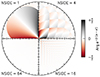 |
Fig. 7. Argument of the phase factor bias e−2i (α − α′) for HEALPix maps with NSIDE = 1, 4, 16, 64, shown in orthographic projection with the north pole at the centre and the equator at the border. The angles α and α′ are defined in Appendix C. For NSIDE = 64, the resolution is at the degree-scale, and the phase factors are close to unity. |
Overall, we expect no impact from neglected phase factors for HEALPix maps with resolution parameter NSIDE ≳ 1024. If necessary, the phase factor bias could be mitigated even further by choosing the coordinate system such that the poles fall into a masked region, e.g. the galactic plane.
6.3. Accuracy
We now validate the results we derive in Sect. 4 with simulations. To characterise the accuracy of our measurement, these require many realisations that, for Euclid, cover a significant fraction of the sky. Usually, lognormal simulations would be the method of choice here; however, the transformations involved in sampling lognormal fields are not exact (Tessore et al. 2023), which adds an element of uncertainty to the validation. Gaussian random fields can be simulated with exactly prescribed two-point statistics; however, for realistic angular power spectra and values of linear galaxy bias, the realised density fields almost surely contain regions where the number density becomes negative. Instead, we use squared Gaussian random fields, which is a toy model we develop in Appendix E that can be simulated exactly and remains physically valid everywhere.
To accurately quantify the effects of map-based measurements, we require simulations that are not themselves affected by pixel effects. We therefore simulate the fields not in real space, but via their spherical harmonic expansion (2). We then sample points using a rejection sampling scheme that accepts or rejects points with a probability that is proportional to the simulated density field, evaluated in each sampled point from the spherical harmonic expansion. Instead of a survey footprint map, we draw points from a spherical cap of 2500 deg2, matching the anticipated area of Euclid’s DR1, and located at the centre of the Euclid Flagship simulation (Euclid Collaboration: Castander et al. 2025). The weak lensing fields are subsequently evaluated at the sampled positions from their spherical harmonic expansions, without any intermediary interpolation.
We then generate 10 000 realisations of these simulations. To show results for both auto- and cross-spectra, we simulate two Gaussian tomographic redshift bins centred on representative redshifts of z = 0.5, 1.0 with a width of σz = 0.125. To simulate galaxy clustering, we use realistic redshift-dependent galaxy bias (Euclid Collaboration: Lepori et al. 2022), with a Euclid-like galaxy density of 2 galaxies per arcmin2 in each tomographic bin. For each simulated galaxy, we store its position, as well as its observed ellipticity from weak lensing with a random intrinsic ellipticity drawn from a hyperbolic normal distribution (Tessore et al. 2023), using a per-component standard deviation σϵ = 0.26. Instead of using the correct weak lensing action (56), we simply sum the intrinsic ellipticity and the shear γ from weak lensing, since we might otherwise pick up biases due to the reduced shear approximation (Deshpande et al. 2020). Finally, we give every galaxy a random shear weight from a log-uniform distribution between 10−2 and 102, to simulate a dynamic range that should exceed any real shear measurement method.
For each simulation, we measure the angular power spectra of the reconstructed density field δ, the cosmic shear E- and B-mode (Appendix D), and their cross-correlations in the two tomographic bins for angular modes up to l = 3000. In addition, we measure the angular power spectra of the visibility V and the shear weight W in each bin for modes up to l = 9000, from which we compute the mixing matrices (25) truncated at l = 3000 and l1 = 6000. By construction, our simulations are band-limited at l = 6000, so that these truncated mixing matrices should contain all non-zero entries, and yield exact expectations for our measurements.
We thus obtain measured and expected angular power spectra for all combinations of probes across the two tomographic bins: angular clustering, cosmic shear, and galaxy–galaxy lensing. To reduce noise, we average the spectra over 32 angular bins with logarithmic spacing between l = 10 and l = 3000. We then compute the mean of the bias ΔCl = Cl − ⟨Cl⟩ between measurements and expectations, which we scale relative to the standard deviation σl of each measurement over the set of realisations.
We carry out the measurements for each simulation using (i) the exact angular power spectra computed from discrete sets of points, and (ii) map-based angular power spectrum from HEALPix maps with resolution parameter NSIDE = 4096. The results are shown in Fig. 8. For the exact, discrete spectra, we find agreement at the 1% level relative to the standard deviation, except for effects that can be ascribed to source–lens clustering (i.e. Assumption 6). For the HEALPix-based spectra, the results show an additional per-cent-level bias in angular clustering at small scales. Further testing reveals that the small-scale HEALPix bias has a dependency on the location of the survey footprint, and we can hence ascribe it to the pseudo-convolution with varying pixel shapes. The dependence of the recovered angular power spectra on pixel shapes is more thoroughly explored elsewhere (Hall & Tessore, in prep.).
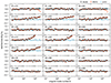 |
Fig. 8. Bias relative to statistical uncertainty between measured and expected angular power spectra from 10 000 simulations with a Euclid DR1-like set-up. Shown are spectra for combinations of galaxy density δ and cosmic shear E- and B-mode in two tomographic bins. The discrete angular power spectra show very good agreement between measurement and expectation (black), except for effects that can be ascribed to source–lens clustering. The same effects are visible for map-based spectra from HEALPix; in addition, these also show a small residual in angular clustering due to the pseudo-convolution of HEALPix pixels (red). When source–lens clustering is taken into account (blue), the relative bias of the discrete spectra is consistent with zero at the 1% level (error bars). Points of the three data sets are slightly offset for better visibility. |
To demonstrate that the bias in Fig. 8 is in fact source–lens clustering, we run a second set of simulations where the positions of shears are distributed according to an independent (but identically clustered) realisation of large-scale structure. When source–lens clustering is thus taken into account, the discrete spectra show a relative bias that is consistent with zero at the 1% level for all probes.
Overall, we find that the HEALPix-based measurements are only marginally biased with respect to the exact discrete angular power spectra. In light of the lower computational cost, we therefore adopt this method for Euclid’s DR1 analysis, which will enable faster turnaround in the data processing. However, since accuracy is a function of survey area and galaxy density, this may no longer be the case for subsequent data releases.
6.4. Applicability to Euclid DR1
To demonstrate that we have a viable pipeline for Euclid’s first data release (DR1), we process a realistic DR1-like data volume. To do so, we select galaxies contained in the provisional northern DR1 footprint (Euclid Collaboration: Scaramella et al. 2022) from the Euclid Flagship simulation (Euclid Collaboration: Castander et al. 2025), obtained from CosmoHub (Tallada et al. 2020; Carretero et al. 2017). The Euclid data processing pipeline aims to support up to 13 tomographic redshift bins (Euclid Collaboration: Mellier et al. 2025), and since the number of spectra and mixing matrices increases quadratically with the number of tomographic bins, we want to ensure compliance with such a setting. Using the simulated photometric redshifts, we therefore bin galaxies into 13 equi-populated tomographic redshift bins. We then measure all 780 possible auto- and cross-correlations between galaxy positions and cosmic shear E- and B-modes. To compare the measurements with expectations, we further compute mixing matrices for all spectra from the simulated visibility and shear weight maps. For this test, we apply the HEALPix-based methodology, with resolution parameter NSIDE = 4096 and maximum angular mode number l = 5000 for all probes, which exceeds the “optimistic” forecast of scale cuts (Euclid Collaboration: Blanchard et al. 2020).
The results are shown in Figs. A.1 and A.2. To compute the expected spectra, we obtain theoretical full-sky predictions with the Cosmology Likelihood for Observables in Euclid code, CLOE (Euclid Collaboration: Joudaki et al., in prep.), using the implemented prescription for photometric harmonic-space observables (Euclid Collaboration: Cardone et al., in prep.). We use HMCode2020 (Mead et al. 2021) to model the non-linear matter power spectrum, as provided in the public code CAMB (Challinor & Lewis 2011). For the background cosmology, we use the same parameter values as in the Euclid Flagship simulation (Euclid Collaboration: Castander et al. 2025). To compute the observables, we use the simulated redshift distributions n(z), and a linear galaxy bias measured from the Euclid Flagship simulation (Euclid Collaboration: Lepori et al. 2022). Since we are only testing the feasibility of the data processing here, we do not perform any fine-tuning of the non-linear modelling, or take into account systematic effects such as magnification bias or intrinsic alignments. This is visible, e.g. in the angular clustering at small scales l ≳ 1000. Nevertheless, we obtain a level of agreement between measurements and expectations that is in line with previous results (Euclid Collaboration: Castander et al. 2025).
Processing the data from DR1-like catalogues to all 780 angular power spectra is very fast: obtaining the spherical harmonic expansions of the fields and weights in one tomographic bin takes around three minutes of wall-clock time, and all tomographic bins can be processed in parallel. The subsequent computation of angular power spectra from all combinations of spherical harmonic coefficients of the fields has negligible cost. Computation of the mixing matrices from the spherical harmonic coefficients of the weights is a more resource-intensive operation, taking around 75 CPU core-hours in total; however, all mixing matrices can be computed in parallel as necessary. Overall, we therefore expect no significant impact on Euclid’s DR1 processing from the measurement of angular power spectra.
7. Discussion and conclusion
We derived a complete framework to obtain the exact measurements and expectations for the angular power spectra from discrete sets of data. Starting from an exact map-free formalism, we find new results such as exact non-stochastic expressions for the additive (noise) biases (36) and (60) for angular clustering and random fields, respectively. Furthermore, by explicitly tracking what assumptions enter our measurements, we are able to separate the methodological accuracy of our results (i.e. when all assumptions are true) from the true accuracy of the results, for example in cases of intrinsic alignments and source–lens clustering, which need to be treated at the level of theoretical predictions. When validating our results on simulations, we find that discrete angular power spectra can achieve biases of less than 1% with respect to their standard deviation in a Euclid DR1-like setting. Overall, we are therefore confident in our ability to measure angular power spectra to the very high level of accuracy required to achieve Euclid’s ambitious science goals.
Using the theory of spherical convolution (86), we can connect our exact theory with the standard practice of measuring angular power spectra from HEALPix maps, for example. Conceptually, this is a step away from the picture in which the observed maps are ‘noisy tracers’ of an underlying continuous field, such as the true galaxy density or the true cosmic shear. In practice, the main difference between the exact map-based formalism and standard practice is that observations are summed over one map pixel (i.e. convolution kernel), but are not averaged. This side-steps common issues with map-based spectra (e.g. empty pixels) or the fact that pixels containing just one single observation point are effectively unweighted after averaging.
When analysing Euclid DR1-like simulations, we find that HEALPix-based spectra can perform at a level of accuracy that is comparable to the discrete spectra. An exception is the case of angular galaxy clustering, where the HEALPix pseudo-convolution, due to varying pixel shapes, introduces a position-dependent bias at the per cent level for angular mode numbers l at or above the resolution parameter NSIDE. However, since this bias is both small and mitigable by relevant analysis choices (i.e. map resolution and scale cuts), we plan to employ the map-based methodology for Euclid’s first data release.
We make our implementation of the methodology presented here available in the form of a code called Heracles1. This code, originally created for 3 × 2 pt data processing in the Euclid Science Ground Segment, was designed from the ground up to be user-friendly and widely applicable to any given probe and survey, and will be maintained for public use.
Generally speaking, homogeneity is invariance under translations, whereas invariance under rotations is isotropy. The translations of the sphere are rotations, and any rotation of the sphere can be achieved by three translations, so that homogeneity and isotropy are equivalent.
In what follows, we always implicitly assume that points have spin-0 weights, since that is the only practically relevant case. However, our results generalise straightforwardly to the spin-weighted case. For unweighted observations, the weights are set to unity.
For simplicity, we use NN′ for the number of pairs here, while the true number of pairs might be slightly different, e.g. N(N − 1) for an auto-correlation. If the difference is significant, one can introduce a pair count correction factor.
The angular correlation function 𝔴 is not to be confused with the weight w.
Here, degenerate pairs refer to observations of the same random field value gk ≡ g′k′. Apart from auto-correlations, such pairs also arise, e.g. for cosmic shear when one set of galaxies is observed with two different shape measurement methods, where it may be the case that gk ≡ g′k′ but ϵk ≠ ϵ′k′ and wk ≠ w′k′.
Not to be confused with the shear in gravitational lensing.
Not to be confused with the cosmological curvature matter density.
The convolution kernel (90) and coefficients (92) follow from the integral (4.11.9) of Varshalovich et al. (1988), which in fact yields a more general, spin-changing convolution kernel with S ≠ s.
The prefix ‘pseudo-’ is used here in the statistical sense, and not to be confused with meaning ‘partial sky’, for which it is unfortunately sometimes also used.
For that reason, the scale parameter λ of a lognormal random variable is commonly called the “shift” parameter (Tessore et al. 2023).
Acknowledgments
We thank Kevin Wolz and David Alonso for their collaboration during the completion of this manuscript. We also thank Ben Wandelt for a number of excellent comments, and the anonymous referee for improving our manuscript. NT thanks Martin Reinecke for pointing out the possibility of implementing the discrete angular power spectrum computation using ducc. This work was supported by UK Space Agency grants ST/W002574/1 and ST/X00208X/1. AH acknowledges support through a Royal Society University Research Fellowship. GCH acknowledges support through the ESA research fellowship programme. This work has made use of CosmoHub, developed by PIC (maintained by IFAE and CIEMAT) in collaboration with ICE-CSIC. CosmoHub received funding from the Spanish government (MCIN/AEI/10.13039/501100011033), the EU NextGeneration/PRTR (PRTR-C17.I1), and the Generalitat de Catalunya. For the purpose of open access, the authors have applied a Creative Commons Attribution (CC BY) licence to any Author Accepted Manuscript version arising from this submission. The Euclid Consortium acknowledges the European Space Agency and a number of agencies and institutes that have supported the development of Euclid, in particular the Agenzia Spaziale Italiana, the Austrian Forschungsförderungsgesellschaft funded through BMK, the Belgian Science Policy, the Canadian Euclid Consortium, the Deutsches Zentrum für Luft-und Raumfahrt, the DTU Space and the Niels Bohr Institute in Denmark, the French Centre National d’Etudes Spatiales, the Fundação para a Ciência e a Tecnologia, the Hungarian Academy of Sciences, the Ministerio de Ciencia, Innovación y Universidades, the National Aeronautics and Space Administration, the National Astronomical Observatory of Japan, the Netherlandse Onderzoekschool Voor Astronomie, the Norwegian Space Agency, the Research Council of Finland, the Romanian Space Agency, the State Secretariat for Education, Research, and Innovation (SERI) at the Swiss Space Office (SSO), and the United Kingdom Space Agency. A complete and detailed list is available on the Euclid website (https://www.euclid-ec.org/).
References
- Abbott, T. M. C., Aguena, M., Alarcon, A., et al. 2022, Phys. Rev. D, 105, 023520 [CrossRef] [Google Scholar]
- Alonso, D., Sanchez, J., Slosar, A., & LSST Dark Energy Science Collaboration 2019, MNRAS, 484, 4127 [NASA ADS] [CrossRef] [Google Scholar]
- Alsing, J., Heavens, A., Jaffe, A. H., et al. 2016, MNRAS, 455, 4452 [Google Scholar]
- Baleato Lizancos, A., & White, M. 2024, JCAP, 05, 010 [Google Scholar]
- Bartelmann, M., & Schneider, P. 2001, Phys. Rep., 340, 291 [Google Scholar]
- Boyle, M. 2016, J. Math. Phys., 57, 092504 [Google Scholar]
- Brown, M. L., Castro, P. G., & Taylor, A. N. 2005, MNRAS, 360, 1262 [NASA ADS] [CrossRef] [Google Scholar]
- Carretero, J., Tallada, P., Casals, J., et al. 2017, Proceedings of the European Physical Society Conference on High Energy Physics, 488 [Google Scholar]
- Challinor, A., & Lewis, A. 2011, Phys. Rev. D, 84, 043516 [NASA ADS] [CrossRef] [Google Scholar]
- Deshpande, A. C., Kitching, T. D., Cardone, V. F., et al. 2020, A&A, 636, A95 [NASA ADS] [CrossRef] [EDP Sciences] [Google Scholar]
- Driscoll, J. R., & Healy, D. M. 1994, Adv. Appl. Math., 15, 202 [Google Scholar]
- Dupac, X., & Tauber, J. 2005, A&A, 430, 363 [NASA ADS] [CrossRef] [EDP Sciences] [Google Scholar]
- Edmonds, A. R. 1960, Angular Momentum in Quantum Mechanics (Princeton: Princeton University Press) [Google Scholar]
- Euclid Collaboration (Blanchard, A., et al.) 2020, A&A, 642, A191 [NASA ADS] [CrossRef] [EDP Sciences] [Google Scholar]
- Euclid Collaboration (Lepori, F., et al.) 2022, A&A, 662, A93 [NASA ADS] [CrossRef] [EDP Sciences] [Google Scholar]
- Euclid Collaboration (Scaramella, R., et al.) 2022, A&A, 662, A112 [NASA ADS] [CrossRef] [EDP Sciences] [Google Scholar]
- Euclid Collaboration (Mellier, Y., et al.) 2025, A&A, in press, https://doi.org/10.1051/0004-6361/202450810 [Google Scholar]
- Euclid Collaboration (Castander, F. J., et al.) 2025, A&A, in press, https://doi.org/10.1051/0004-6361/202450853 [Google Scholar]
- Górski, K. M., Hivon, E., Banday, A. J., et al. 2005, ApJ, 622, 759 [Google Scholar]
- Heavens, A. F., & Taylor, A. N. 1995, MNRAS, 275, 483 [NASA ADS] [Google Scholar]
- Heymans, C., Tröster, T., Asgari, M., et al. 2021, A&A, 646, A140 [NASA ADS] [CrossRef] [EDP Sciences] [Google Scholar]
- Hikage, C., Takada, M., Hamana, T., & Spergel, D. 2011, MNRAS, 412, 65 [NASA ADS] [CrossRef] [Google Scholar]
- Hikage, C., Oguri, M., Hamana, T., et al. 2019, PASJ, 71, 43 [Google Scholar]
- Hilbert, S., Hartlap, J., & Schneider, P. 2011, A&A, 536, A85 [NASA ADS] [CrossRef] [EDP Sciences] [Google Scholar]
- Hivon, E., Górski, K. M., Netterfield, C. B., et al. 2002, ApJ, 567, 2 [NASA ADS] [CrossRef] [Google Scholar]
- Huffenberger, K. M., & Wandelt, B. D. 2010, ApJS, 189, 255 [NASA ADS] [CrossRef] [Google Scholar]
- Joachimi, B., Cacciato, M., Kitching, T. D., et al. 2015, Space Sci. Rev., 193, 1 [Google Scholar]
- Joachimi, B., Lin, C. A., Asgari, M., et al. 2021, A&A, 646, A129 [NASA ADS] [CrossRef] [EDP Sciences] [Google Scholar]
- Johnston, H., Wright, A. H., Joachimi, B., et al. 2021, A&A, 648, A98 [NASA ADS] [CrossRef] [EDP Sciences] [Google Scholar]
- Kamionkowski, M., Kosowsky, A., & Stebbins, A. 1997, Phys. Rev. D, 55, 7368 [NASA ADS] [CrossRef] [Google Scholar]
- Kerscher, M., Szapudi, I., & Szalay, A. S. 2000, ApJ, 535, L13 [NASA ADS] [CrossRef] [Google Scholar]
- Kiessling, A., Cacciato, M., Joachimi, B., et al. 2015, Space Sci. Rev., 193, 67 [Google Scholar]
- Kirk, D., Brown, M. L., Hoekstra, H., et al. 2015, Space Sci. Rev., 193, 139 [Google Scholar]
- Kitching, T. D., & Deshpande, A. C. 2022, Open J. Astrophys., 5, 6 [NASA ADS] [CrossRef] [Google Scholar]
- Kitching, T., Deshpande, A., & Taylor, P. 2021, Open J. Astrophys., 4, 17 [NASA ADS] [CrossRef] [Google Scholar]
- Landy, S. D., & Szalay, A. S. 1993, ApJ, 412, 64 [Google Scholar]
- Laureijs, R., Amiaux, J., Arduini, S., et al. 2011, ArXiv e-prints [arXiv:1110.3193] [Google Scholar]
- Linke, L., Unruh, S., Wittje, A., et al. 2024, ArXiv e-prints [arXiv:2407.09810] [Google Scholar]
- Loureiro, A., Whiteway, L., Sellentin, E., et al. 2023, Open J. Astrophys., 6, 6 [CrossRef] [Google Scholar]
- Maraio, A., Hall, A., & Taylor, A. 2023, MNRAS, 520, 4836 [NASA ADS] [CrossRef] [Google Scholar]
- McEwen, J. D., & Wiaux, Y. 2011, IEEE Trans. Signal Process., 59, 5876 [Google Scholar]
- McEwen, J. D., Leistedt, B., Büttner, M., Peiris, H. V., & Wiaux, Y. 2015, ArXiv e-prints [arXiv:1509.06749] [Google Scholar]
- Mead, A. J., Brieden, S., Tröster, T., & Heymans, C. 2021, MNRAS, 502, 1401 [Google Scholar]
- More, S., Sugiyama, S., Miyatake, H., et al. 2023, Phys. Rev. D, 108, 123520 [NASA ADS] [CrossRef] [Google Scholar]
- Nicola, A., García-García, C., Alonso, D., et al. 2021, JCAP, 03, 067 [Google Scholar]
- Peebles, P. J. E. 1973, ApJ, 185, 413 [Google Scholar]
- Percival, W. J., Burkey, D., Heavens, A., et al. 2004, MNRAS, 353, 1201 [NASA ADS] [CrossRef] [Google Scholar]
- Reinecke, M., Belkner, S., & Carron, J. 2023, A&A, 678, A165 [NASA ADS] [CrossRef] [EDP Sciences] [Google Scholar]
- Rodríguez-Monroy, M., Weaverdyck, N., Elvin-Poole, J., et al. 2022, MNRAS, 511, 2665 [CrossRef] [Google Scholar]
- Schneider, P., van Waerbeke, L., Kilbinger, M., & Mellier, Y. 2002, A&A, 396, 1 [NASA ADS] [CrossRef] [EDP Sciences] [Google Scholar]
- Schneider, P., Eifler, T., & Krause, E. 2010, A&A, 520, A116 [NASA ADS] [CrossRef] [EDP Sciences] [Google Scholar]
- Seitz, C., & Schneider, P. 1997, A&A, 318, 687 [NASA ADS] [Google Scholar]
- Sellentin, E., Loureiro, A., Whiteway, L., et al. 2023, Open J. Astrophys., 6, 31 [Google Scholar]
- Singh, S., Mandelbaum, R., Seljak, U., Slosar, A., & Vazquez Gonzalez, J. 2017, MNRAS, 471, 3827 [Google Scholar]
- Tadros, H., Ballinger, W. E., Taylor, A. N., et al. 1999, MNRAS, 305, 527 [NASA ADS] [CrossRef] [Google Scholar]
- Tallada, P., Carretero, J., Casals, J., et al. 2020, Astron. Comput., 32, 100391 [Google Scholar]
- Tegmark, M. 1997, Phys. Rev. D, 55, 5895 [NASA ADS] [CrossRef] [Google Scholar]
- Tegmark, M., & de Oliveira-Costa, A. 2001, Phys. Rev. D, 64, 063001 [Google Scholar]
- Tessore, N., Loureiro, A., Joachimi, B., von Wietersheim-Kramsta, M., & Jeffrey, N. 2023, Open J. Astrophys., 6, 11 [NASA ADS] [CrossRef] [Google Scholar]
- Troxel, M. A., & Ishak, M. 2015, Phys. Rep., 558, 1 [NASA ADS] [CrossRef] [Google Scholar]
- Varshalovich, D. A., Moskalev, A. N., & Khersonskii, V. K. 1988, Quantum Theory of Angular Momentum (World Scientific) [CrossRef] [Google Scholar]
- Wandelt, B. D., & Górski, K. M. 2001, Phys. Rev. D, 63, 123002 [NASA ADS] [CrossRef] [Google Scholar]
- Wandelt, B. D., Hivon, E., & Górski, K. M. 2001, Phys. Rev. D, 64, 083003 [NASA ADS] [CrossRef] [Google Scholar]
- Wolz, K., Alonso, D., & Nicola, A. 2025, J. Cosmol. Astropart. Phys., 2025, 028 [Google Scholar]
- Zaldarriaga, M., & Seljak, U. 1997, Phys. Rev. D, 55, 1830 [Google Scholar]
Appendix A: Additional figures
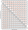 |
Fig. A.1. Angular power spectra (red) for angular clustering (upper triangle) and cosmic shear (lower triangle) in the Euclid Flagship simulation with a DR1-like footprint. For cosmic shear, the B-mode spectrum due to mode mixing is shown in blue. Also shown is the expectation for each spectrum (dashed), as computed from the respective mixing matrices. All spectra are binned into 32 angular bins with logarithmic spacing between l = 10 and l = 5000. The y-axis changes to linear scaling when passing through the origin. |
Appendix B: Alternative estimators for angular clustering
In Sect. 4.1, we measure the two-point statistics for point processes using the particular choice of density contrast (50). Here, we consider a number of alternative choices.
Firstly, we can trivially replace the mean number density  by a catalogue of random points (‘randoms’). Given the definition (42) of the mean number density, these randoms must be distributed according to the visibility v (Baleato Lizancos & White 2024).
Secondly, in full correspondence to real-space methods, we can directly construct estimators of the angular power spectrum 𝔴l from the expectation (49). For example, using a formal inverse  of the mixing matrix, we can construct the estimator
![Mathematical equation: $$ \begin{aligned} \hat{\mathfrak{w} }_l^{\mathrm{N} } = \sum _{l^{\prime }} (M^{\bar{n}\bar{n}^{\prime }})^{-1}_{ll^{\prime }} \, \Bigl [ C_{l^{\prime }}^{nn^{\prime }} - C_{l^{\prime }}^{\bar{n}\bar{n}^{\prime }} - A^{nn^{\prime }}\Bigr ]. \end{aligned} $$](/articles/aa/full_html/2025/02/aa52018-24/aa52018-24-eq218.gif) (B.1)
(B.1)
In the taxonomy of Kerscher et al. (2000), this corresponds to the “natural” real-space estimator (DD − RR)/RR. Furthermore, by expectation (44), we have  , and we can hence construct a more advanced estimator
![Mathematical equation: $$ \begin{aligned} \hat{\mathfrak{w} }_l^{\mathrm{LS} } = \sum _{l^{\prime }} (M^{\bar{n}\bar{n}^{\prime }})^{-1}_{ll^{\prime }} \, \Bigl [C_{l^{\prime }}^{nn^{\prime }} - C_{l^{\prime }}^{n\bar{n}^{\prime }} - C_{l^{\prime }}^{\bar{n}n^{\prime }} + C_{l^{\prime }}^{\bar{n}\bar{n}^{\prime }} - A^{nn^{\prime }}\Bigr ]. \end{aligned} $$](/articles/aa/full_html/2025/02/aa52018-24/aa52018-24-eq220.gif) (B.2)
(B.2)
This is the harmonic-space equivalent of the Landy & Szalay (1993) estimator (DD − DR − RD + RR)/RR.
The estimators (B.1) and (B.2) both rely on inversion of the mixing matrix. We can similarly construct a partial-sky variant of the natural estimator in harmonic space,
 (B.3)
(B.3)
as well as a partial-sky variant of the harmonic-space Landy-Szalay estimator,
 (B.4)
(B.4)
The respective expectation of both partial-sky estimators is the product of mixing matrix and full-sky expectation. In particular, the partial-sky Landy–Szalay estimator (B.4) is essentially the same as the measured angular power spectrum (51) of the density contrast (50).
Lastly, to see why we normalise the density contrast (50) by a constant  , consider an alternative definition of the density contrast with an arbitrary normalisation function q,
 (B.5)
(B.5)
It follows from the definitions of the number density (28) and mean number density (42) that δq is equivalent to δ under a change of weights  and, consequently, a change of visibility
  . Defining the density contrast (50) with a different normalisation therefore effectively replaces the given set of weights with a different set of weights.
Appendix C: Relative orientation on the sphere
To obtain the angles α and α′ that describe the relative orientation of points  and
and  on the sphere, it suffices to solve the spherical triangle shown in Fig. C.1 (for more information, see Hall & Tessore in prep.),
 (C.1)
(C.1)
 (C.2)
(C.2)
The respective numerators and denominators are written here such that their signs yield the correct quadrant for the inverse tangent.
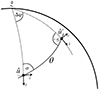 |
Fig. C.1. Angles α, θ, α′ that describe the relative orientation between two points |


The same angles can be expressed in terms of the components of the unit vectors  and
and  as
as
 (C.3)
(C.3)
 (C.4)
(C.4)
with  . This form is often useful in applications where points are available as vectors, since it requires no additional trigonometric operations. In fact, for α = arctan(q/p), we find a familiar expression for the spin-2 phase factors that appear, e.g. in the spherical harmonic addition theorem (8),
 (C.5)
(C.5)
The phase factors can hence be computed entirely in terms of the vector components of  and
and  .
.
Appendix D: Decomposition into E- and B-modes
If the spherical function f is a complex-valued random field, the two-point statistics of f and a second, not necessarily distinct, field f′ are not fully characterised by the expected angular correlations (16) alone. Like for any complex random variable, we also require the associated pseudo-correlation ⟨Cf*f′(θ)⟩, i.e. the correlation of the complex conjugated random field f* and f′,
 (D.1)
(D.1)
where we have used the fact that the spin weight of f* is −s. The same information is contained in the pseudo-spectrum11
 (D.2)
(D.2)
which is merely expectation (13) applied to f* and f′.
Instead of using spectra and pseudo-spectra, it is often more convenient to work with a different decomposition of the harmonic-space two-point statistics, namely that into E- and B-modes (Zaldarriaga & Seljak 1997). For a spherical function f with spin weight s, the respective E- and B-modes are defined as linear combinations of the spherical harmonic coefficients of f and f*,
 (D.3)
(D.3)
 (D.4)
(D.4)
where the overall negative sign is the convention adopted by HEALPix. The E- and B-mode spectra are then obtained by using Elm and Blm in the angular power spectrum (9). Since the coefficients (D.3) and (D.4) are linear combinations of flm and (f*)lm, it is clear that the resulting E- and B-mode spectra are linear combinations of the spectra Clff′, Clf*f′, etc. of the constituent fields and their complex conjugates.
To compute, e.g. the expectation for partial-sky E- and B-mode spectra, it therefore suffices to apply the mixing matrix formalism described above to the individual spectra of the fields, and express the result in terms of the full-sky E- and B-mode spectra. In doing so, one finds that the mixing matrices also introduce mixing between E- and B-modes (Brown et al. 2005).
Appendix E: Squared normal fields
In this section we consider a Gaussian random field X on the sphere that is transformed into a random field Y by an arbitrary function t,
 (E.1)
(E.1)
As shown by Tessore et al. (2023), a band-limited angular power spectrum Gl for X does not generally result in a band-limited angular power spectrum Cl for Y. In practice, we are not generally able to construct a spectrum Gl that, after transformation, reproduces a desired spectrum Cl exactly. For validation, we now try and identify a special case where that is possible. In particular, we look for a transformation with the following two characteristics:
-
i)
The transformed field Y is bounded from below, so that we can simulate density contrasts δ for angular clustering that respect the physical bound δ ≥ −1.
-
ii)
The transformed field Y has a band-limited spectrum.
Lognormal fields satisfy the first criterium, but lack a strictly band-limited spectrum. However, it turns out that both criteria are fulfilled by squaring a Gaussian random field.
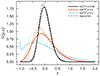 |
Fig. E.1. Shape of squared normal distributions (solid) and lognormal distributions with the same variance (dashed). For small variances, the distribution is approximately normal (black). For large variances, the distribution saturates at its lower bound (blue). In the intermediate regime, the distribution has a roughly lognormal shape (red). |
Let X be a normal random variable with zero mean and variance σ2 ≤ 1, and let  . Define the random variable Y as a quadratic transformation of X, resulting in a scaled and shifted non-central χ2 random variable with 1 degree of freedom,
![Mathematical equation: $$ \begin{aligned} Y = \lambda \, [(X - a)^2 - 1], \end{aligned} $$](/articles/aa/full_html/2025/02/aa52018-24/aa52018-24-eq249.gif) (E.2)
(E.2)
where λ > 0 is the scale parameter of the distribution, which also fixes the minimum value of Y.12 A straightforward calculation shows that Y has zero mean and variance
 (E.3)
(E.3)
Inserting σ2 = 1 − a2, the variance can equivalently be expressed in terms of a,
 (E.4)
(E.4)
and the value of a can hence be obtained from the variance of the transformed random variable,
 (E.5)
(E.5)
The transformation (E.2) is therefore readily obtained in either direction. Setting λ = 1, the standardised probability distribution function of Y is
 (E.6)
(E.6)
The distribution approaches normality for small variances, and becomes more skewed as the variance increases, similar to the lognormal distribution (Fig. E.1).
We then apply the transformation (E.2) pointwise to a pair X and X′ of jointly homogeneous Gaussian random fields on the sphere. By expectation (16), there is a correlation function G such that  . It can be shown that the transformed fields Y and Y′ are also jointly homogeneous (Tessore et al. 2023), and there is hence an angular correlation function C such that
  . Using the transformation (E.2), we can compute C(θ) in terms of G(θ),
 (E.7)
(E.7)
By completing the square, we also obtain the inverse relation,
 (E.8)
(E.8)
Furthermore, relation (E.7) is readily transformed to harmonic space using expectation (24),
 (E.9)
(E.9)
Since the triangle condition l ≤ l1 + l2 is imposed on the sum by the Wigner 3j symbols, it follows that Cl is indeed band-limited if Gl is band-limited, at twice the angular mode number. In this case, the non-linear solver for Gl proposed by Tessore et al. (2023) can produce an essentially exact transformation.
For our simulations, the variance of each random field, and hence a, is determined by its spectrum. It remains to fix the value of λ. For angular clustering, we simulate the density contrast δ, for which we set λ = 1. For cosmic shear, we simulate the convergence field κ, for which we set λ using the fitting formula of Hilbert et al. (2011).
All Figures
|
Fig. 1. Overview of the methodology presented below. We apply the formalism for discrete angular power spectra in three distinct ways: (i) Exact spherical harmonic coefficients can be computed from the discrete data, without the use of maps. In turn, angular power spectra can be computed from combinations of spherical harmonic coefficients. (ii) The angular power spectra themselves can be computed from the discrete data. This is inefficient for practical computation, but makes it possible to obtain exact expressions for the expected spectra. (iii) The discrete data can be turned into maps, and subsequently into spherical harmonic coefficients by means of a spherical harmonic transform. This can yield the same results as the discrete transformation. |
| In the text | |
|
Fig. 2. Convolution kernel (90) with no cut-off for spin weight s = 0 (black) and spin weight s = 2 (red). For sufficiently small angles the convolution kernel becomes indistinguishable from a flat spherical disc even in the spin-weighted case. |
| In the text | |
|
Fig. 3. Normalised coefficients of the convolution kernel (90) for spin weights s = 0 (black), s = 2 (red), and kernel sizes β = 10° (top), β = 1° (middle), β = 1 arcmin (bottom). There is excellent agreement between the coefficients for s = 2 and s = 0, except in the case of a large kernel (β = 10°) at large angular scales (l < 10). |
| In the text | |
|
Fig. 4. HEALPix pixel window function (red) for resolution parameters NSIDE = 256 (top), NSIDE = 1024 (middle), NSIDE = 4096 (bottom). Also shown is the convolution kernel of a spherical disc with the same pixel area (black). The HEALPix pixel window function is only provided up to l = 4 NSIDE, where it starts to fall below the kernel of the spherical disc. |
| In the text | |
|
Fig. 5. Angular power spectrum of 1 000 000 uniform random points, computed using the HEALPix pseudo-convolution (red) and a true convolution with spherical discs of the same area (black). Both results agree with their respective expectation (dashed). The convolution kernel is only imprinted on the true convolution. |
| In the text | |
|
Fig. 6. Simulated distribution of the relative error when estimating the mean density |
| In the text | |
|
Fig. 7. Argument of the phase factor bias e−2i (α − α′) for HEALPix maps with NSIDE = 1, 4, 16, 64, shown in orthographic projection with the north pole at the centre and the equator at the border. The angles α and α′ are defined in Appendix C. For NSIDE = 64, the resolution is at the degree-scale, and the phase factors are close to unity. |
| In the text | |
|
Fig. 8. Bias relative to statistical uncertainty between measured and expected angular power spectra from 10 000 simulations with a Euclid DR1-like set-up. Shown are spectra for combinations of galaxy density δ and cosmic shear E- and B-mode in two tomographic bins. The discrete angular power spectra show very good agreement between measurement and expectation (black), except for effects that can be ascribed to source–lens clustering. The same effects are visible for map-based spectra from HEALPix; in addition, these also show a small residual in angular clustering due to the pseudo-convolution of HEALPix pixels (red). When source–lens clustering is taken into account (blue), the relative bias of the discrete spectra is consistent with zero at the 1% level (error bars). Points of the three data sets are slightly offset for better visibility. |
| In the text | |
|
Fig. A.1. Angular power spectra (red) for angular clustering (upper triangle) and cosmic shear (lower triangle) in the Euclid Flagship simulation with a DR1-like footprint. For cosmic shear, the B-mode spectrum due to mode mixing is shown in blue. Also shown is the expectation for each spectrum (dashed), as computed from the respective mixing matrices. All spectra are binned into 32 angular bins with logarithmic spacing between l = 10 and l = 5000. The y-axis changes to linear scaling when passing through the origin. |
| In the text | |
 |
Fig. A.2. Same as Fig. A.1, but for galaxy–galaxy lensing. |
| In the text | |
|
Fig. C.1. Angles α, θ, α′ that describe the relative orientation between two points |
| In the text | |
|
Fig. E.1. Shape of squared normal distributions (solid) and lognormal distributions with the same variance (dashed). For small variances, the distribution is approximately normal (black). For large variances, the distribution saturates at its lower bound (blue). In the intermediate regime, the distribution has a roughly lognormal shape (red). |
| In the text | |
Current usage metrics show cumulative count of Article Views (full-text article views including HTML views, PDF and ePub downloads, according to the available data) and Abstracts Views on Vision4Press platform.
Data correspond to usage on the plateform after 2015. The current usage metrics is available 48-96 hours after online publication and is updated daily on week days.
Initial download of the metrics may take a while.