| Issue |
A&A
Volume 692, December 2024
|
|
|---|---|---|
| Article Number | A199 | |
| Number of page(s) | 10 | |
| Section | Numerical methods and codes | |
| DOI | https://doi.org/10.1051/0004-6361/202451663 | |
| Published online | 13 December 2024 | |
Automated detection of satellite trails in ground-based observations using U-Net and Hough transform
1
Department of Astrophysics/IMAPP, Radboud University,
PO Box 9010,
6500 GL
Nijmegen,
The Netherlands
2
Department of Mathematics/IMAPP, Radboud University,
PO Box 9010,
6500 GL
Nijmegen,
The Netherlands
3
Department of Astronomy and Inter-University Institute for Data Intensive Astronomy, University of Cape Town,
Private Bag X3,
Rondebosch
7701,
South Africa
4
South African Astronomical Observatory,
PO Box 9,
Observatory,
7935,
South Africa
5
Leiden Observatory, Leiden University,
Postbus 9513,
2300 RA
Leiden,
The Netherlands
6
Department of Physics, University of Oxford,
Denys Wilkinson Building, Keble Road,
Oxford
OX1 3RH,
UK
★ Corresponding author; This email address is being protected from spambots. You need JavaScript enabled to view it.
Received:
25
July
2024
Accepted:
7
November
2024
Abstract
Aims. The expansion of satellite constellations poses a significant challenge to optical ground-based astronomical observations, as satellite trails degrade observational data and compromise research quality. Addressing these challenges requires developing robust detection methods to enhance data processing pipelines, creating a reliable approach for detecting and analyzing satellite trails that can be easily reproduced and applied by other observatories and data processing groups.
Methods. Our method, called ASTA (Automated Satellite Tracking for Astronomy), combined deep learning and computer vision techniques for effective satellite trail detection. It employed a U-Net based deep learning network to initially detect trails, followed by a probabilistic Hough transform to refine the output. ASTA’s U-Net model was trained on a dataset of manually labeled full-field MeerLICHT telescope images prepared using the user-friendly LABKIT annotation tool. This approach ensured high-quality and precise annotations while facilitating quick and efficient data refinements, which streamlined the overall model development process. The thorough annotation process was crucial for the model to effectively learn the characteristics of satellite trails and generalize its detection capabilities to new, unseen data.
Results. The U-Net performance was evaluated on a test set of 20 000 image patches, both with and without satellite trails, achieving approximately 0.94 precision and 0.94 recall at the selected threshold. For each detected satellite, ASTA demonstrated a high detection efficiency, recovering approximately 97% of the pixels in the trails, resulting in a False Negative Rate (FNR) of only 0.03. When applied to around 200 000 full-field MeerLICHT images focusing on Geostationary (GEO) and Geosynchronous (GES) satellites, ASTA identified 1742 trails −19.1% of the detected trails – that could not be matched to any objects in public satellite catalogs. This indicates the potential discovery of previously uncatalogued satellites or debris, confirming ASTA’s effectiveness in both identifying known satellites and uncovering new objects.
Key words: methods: data analysis / techniques: image processing / astronomical databases: miscellaneous
© The Authors 2024
 Open Access article, published by EDP Sciences, under the terms of the Creative Commons Attribution License (https://creativecommons.org/licenses/by/4.0), which permits unrestricted use, distribution, and reproduction in any medium, provided the original work is properly cited.
This article is published in open access under the Subscribe to Open model. This email address is being protected from spambots. You need JavaScript enabled to view it. to support open access publication.
1 Introduction
The rise of large satellite constellations has greatly enhanced global communication and connectivity. However, this development introduces significant challenges for ground-based telescopes, as satellite trails appear as streaks of light in astronomical images, degrading data quality by introducing noise and covering celestial objects (McDowell 2020). Historically, astronomical observations have faced various sources of interference, but the rapid increase in satellite launches, especially with megaconstellations such as Starlink and OneWeb, has exacerbated the issue (Tyson et al. 2020; Hainaut & Williams 2020; Mallama 2022; Bassa et al. 2022; Gallozzi et al. 2020; Groot 2022). Even space-based observatories, such as the Hubble Space Telescope, are not immune to these effects, highlighting the pervasive nature of satellite interference (Kruk et al. 2023).
The anticipated surge in satellite deployments can significantly increase the frequency and severity of interference, underscoring the need for proactive measures and innovative solutions to ensure the continued effectiveness of ground-based astronomy (Walker et al. 2020). Despite their advanced capabilities, wide-field optical ground-based telescopes, such as ATLAS (Tonry et al. 2018), GOTO (Steeghs et al. 2022), BlackGEM (Groot et al. 2024), ZTF (Bellm et al. 2019), and Pan-STARRS (Chambers et al. 2016), face significant challenges due to the increasing presence of satellite trails in their observations. Upcoming large aperture and wide field-of-view facilities like the Vera Rubin Observatory (Ivezic et al. 2019) will be even more affected by these bright satellite trails. These streaks introduce noise and can obscure celestial objects, complicating the detection and analysis of transient events (see e.g., Groot 2022).
Currently, several methods are employed to detect and mitigate satellite trails in astronomical images. These methods can be broadly categorized into simple source detection, template fitting to line shapes, computer vision techniques, and machine learning algorithms. Simple source detection, such as using SExtractor (Bertin & Arnouts 1996) and focusing on elongated shapes, has been employed to detect streaks. However, this approach is less effective at low signal-to-noise ratios (SNR) and tends to result in a high false-alarm rate (Waszczak et al. 2017). In contrast, template fitting to line shapes involves aligning a predefined streak shape to the image data and calculating a weighted sum of the pixels along the line to assess the match quality. This matched-filter approach (Turin 1960), used by Dawson et al. (2016), employs the maximum likelihood method to detect streaks, assuming uncorrelated noise and a constant known Point Spread Function (PSF). While accurate, it can be computationally intensive and may require multiple templates or faster computational techniques.
Computer vision techniques provide another set of tools for streak detection, using methods developed for natural image processing. These techniques are attractive due to their versatility and effectiveness in various imaging contexts. Two popular methods are the Hough transform (Duda & Hart 1972) and the Radon transform (Radon 1986). The Hough transform is applied to binary images following edge detection, while the Radon transform is used on grayscale images. Despite their different applications, both methods have been successful in finding streaks in crowded fields and images with diffuse light sources (Cheselka 1999; Virtanen et al. 2014; Bekteševic & Vinkovic 2017). Both the Hough transform and the Radon transform have seen improvements in computational efficiency with the development of the probabilistic Hough transform and the Fast Radon transform (FRT), respectively. These advanced methods, which often leverage GPUs, provide significant improvements in speed and computational performance (Zimmer et al. 2013; Andersson et al. 2016; Nir et al. 2018; Borncamp & Lian Lim 2019). A conceptual enhancement to the standard Radon transform, the Median Radon transform (MRT), was recently introduced by Stark et al. (2022). Unlike the traditional approach that sums values along all paths across an image, MRT calculates the median. This method minimizes the influence of non-linear features such as stars and galaxies, resulting in significant sensitivity gains compared to previous techniques.
Despite recent progress, there remains a need for methods that can handle the increasing complexity and volume of astronomical data. Deep learning, in particular, offers new opportunities for improving streak detection. By training convolutional neural networks (CNNs, LeCun et al. 1999) on large datasets of labeled images, these methods can learn complex patterns and features directly from data, improving detection rates and reducing false positives (Paillassa et al. 2020; Elhakiem et al. 2023; Chatterjee et al. 2024). Building on these advancements, our study introduces ASTA (Automated Satellite Tracking for Astronomy), a novel tool that uniquely combines the strengths of deep learning and computer vision techniques for detecting satellite trails in ground-based observations. We used a U-Net architecture (Ronneberger et al. 2015) for initial satellite streak detection, followed by a probabilistic Hough transform to refine the output and extract satellite information.
A common criticism of machine learning methods is the difficulty in obtaining high-quality and well-labeled training sets, which are crucial for achieving accuracy and reliability. This issue often hinders the widespread adoption and reproducibility of such methods. However, we have addressed this challenge by using the LABKIT tool (Arzt et al. 2022) to meticulously annotate images from the MeerLICHT telescope (Bloemen et al. 2016), ensuring the high-quality training data necessary for effective model training. This approach not only produces a reliable dataset for our application but also simplifies the creation process, making it accessible to other researchers and observatories. By providing a detailed account of our methodology and dataset preparation, we aim to facilitate the widespread adoption of ASTA, enhancing the ability of observatories worldwide to mitigate the impact of satellite trails on astronomical data quality.
The paper is organized as follows: Section 2 describes the data and the process of image selection and preparation. Section 3 outlines the machine learning techniques and the probabilistic Hough transform used for refining the detections, along with their validation. Section 4 demonstrates the application of our tool, ASTA, by searching for Geostationary and Geosynchronous satellites in approximately 200 000 full-field MeerLICHT images. This analysis focuses on identifying satellite trails and cross-referencing the results with known public satellite catalogs. Finally, Section 5 summarizes our key findings and discusses the significance of developing sustainable solutions to ensure the advancement of astronomical research in the era of satellite constellations.
ASTA is directly accessible on GitHub1. All the images and masks used in this paper for training, test, and validation are available on Zenodo2 (Stoppa 2024).
2 Data
This study uses data from the MeerLICHT telescope located in South Africa. MeerLICHT, a prototype for the recently operational BlackGEM telescope array (Groot et al. 2024), plays a crucial role in detecting and analyzing transient astronomical phenomena. Both MeerLICHT and BlackGEM are designed to capture high-quality astronomical data, but their ground-based nature makes them susceptible to satellite trails, which can degrade the quality of the data and impact the accurate analysis and interpretation of transient events.
In this section, we explain the data used to create ASTA and the dataset-building process. This involves selecting, preparing, and manually labeling images to ensure high-quality training data for our machine learning algorithm.
2.1 MeerLICHT and BlackGEM telescopes array
The MeerLICHT telescope, with its 65 cm aperture and a high- resolution 10.5k × 10.5k pixel CCD, offers a wide field-of-view of 2.7 square degrees, sampled at 0.56′/pixel. MeerLICHT is equipped with the Sloan-Gunn type u, g, r, i, z filter set, along with an additional wide-band q filter (440–720 nm), enhancing its observational versatility. The telescope uses 60s integrations by default and reaches a limiting point-source magnitude of qAB > 20.5 under standard conditions. As a consequence, any satellite in Low Earth Orbit (LEO) up to Geostationary orbit (GEO) is very well detected and causes strong streaks in the observations. This causes interference in the photometric measurements of astrophysical objects but, at the same time, offers the opportunity to monitor the satellite’s presence in Earth’s orbit.
Images captured by MeerLICHT are promptly processed at the IDIA/ilifu facility using BlackBOX3 image processing software (Vreeswijk et al., in prep). The processing pipeline includes source detection via SourceExtractor (Bertin & Arnouts 1996), astrometric and photometric calibration (Lang et al. 2010), PSF determination (Bertin 2011), image subtraction, and transient detection (Zackay et al. 2016; Hosenie et al. 2021). Furthermore, a new set of deep learning methods has been developed specifically for the MeerLICHT/BlackGEM telescopes. These methods are currently being tested and compared against traditional pixelbased counterpart techniques as detailed in Stoppa et al. (2022, 2023c,a).
Figure 1 illustrates a typical full-field MeerLICHT image, showcasing the impact of multiple satellite trails.
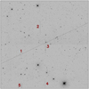 |
Fig. 1 Full-field, 10560 × 10560 pixels, MeerLICHT image with a 60- second exposure, showcasing five satellite trails overlaying dozens of sources. |
2.2 Dataset preparation
Creating a high-quality training dataset is fundamental for developing an effective machine learning model. In our study, we require an accurately labeled dataset where pixels belonging to a satellite trail are assigned to one class, and all other pixels – including those representing the sky background, stars, and common linear artifacts seen in CCD images, such as diffraction spikes, cosmic ray hits, and charge bleeding – are assigned to another class. With such a dataset, the network can effectively learn the relationship between the original image and the segmentation mask, enabling accurate and reliable detection of satellite trails.
However, a significant challenge for researchers attempting to reproduce machine learning methods for their specific applications is the lack of a well-labeled dataset and uncertainty about how to create one from scratch. This obstacle often discourages the adoption of machine learning techniques. To address this issue, we provide a detailed explanation of how to build a reliable dataset for satellite trail detection, offering a clear guide for other researchers and observatories.
We started by collecting 178 full-field MeerLICHT images, all visually inspected to identify the presence of satellite trails. These images included trails of varying lengths and SNRs4. Specifically, the SNR of the trails in our training set ranged from as low as 1.25, which is really close to the background noise level, up to 180, with a median SNR of 11. This wide range allows the model to learn to detect both faint and bright trails, ensuring its sensitivity to trails near the detection limit. The lengths of the trails also varied significantly, from as short as 380 pixels for trails partially captured in the image due to entering or exiting the field of view, up to 14 000 pixels for trails that span the entire image, such as those caused by LEO satellites.
To facilitate the creation of the ground truth segmentation masks, we used LABKIT (Arzt et al. 2022), a plugin for the Fiji image processing package, which simplifies the annotation process with its pixel classification algorithm for quick automatic segmentation. In LABKIT, we first manually classified a really small subset of pixels in the images (~0.001%) into two classes: satellite trails and background. This initial step involved selecting pixels that represent the trails and marking the sky background, sources, and other linear features as background. LABKIT then used these labeled pixels to train a random forest classifier. For each pixel in the image, LABKIT automatically computes a set of values by applying various image processing filters, such as Gaussian blurs, difference of Gaussians, and Laplacian operators. These filters emphasize different aspects of the input image, and their responses for each pixel are combined to form a feature vector. The collection of these feature vectors, paired with their respective ground-truth classes, constitutes the training set for the random forest, which consists of a hundred decision trees. LABKIT then proceeds to predict the segmentation mask for the entire image and provides a quick, although rough, approximation of all the trails.
After LABKIT’s initial automated classification, the software easily provides tools to manually refine the annotations to ensure their accuracy and reliability. Using LABKIT’s interface, we adjusted the pixels and specific parts of trails or spurious detections that were assigned to the wrong class. This comprehensive annotation process resulted in a full binary mask for each full-field MeerLICHT image and was completed by a single person in three days.
After labeling, the full-field images and their associated ground truth masks were divided into smaller patches of 528x528 pixels to facilitate efficient training. Data augmentation techniques, including 90-degree rotations, flips, and shifts, were applied exclusively to patches containing satellite trails. This approach enhanced the model’s exposure to diverse trail characteristics, thereby improving detection accuracy. This selective augmentation was necessary to prevent the dataset from becoming unbalanced, as most patches from a full-field image do not contain satellite trails. Without this, the dataset would be dominated by patches with empty masks, making the model training more difficult and less effective.
Figure 2 shows four examples of patches with satellite trails and their corresponding ground truth masks. As can be seen in Fig. 2, MeerLICHT’s spatial resolution is high enough that seeing- and tracking-variations during the integration can be seen as a ‘wavy’ nature of the trail, making them significantly deviate from just a straight line.
3 Method
This section outlines the methodology employed by ASTA for detecting and analyzing satellite trails in astronomical images. ASTA leverages a U-Net architecture for the initial segmentation of satellite trails, providing a robust framework for distinguishing trails from other features. To enhance the precision of trail delineation, the initial segmentation is refined using the probabilistic Hough transform (Galamhos et al. 1999). This combination of deep learning and classical image processing techniques ensures high accuracy and reliability in identifying and characterizing satellite trails.
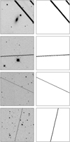 |
Fig. 2 Examples of satellite trail annotations in MeerLICHT images. The figure shows two columns and four rows: (a) original images with satellite trails of varying intensities and types in the first column, (b) corresponding labeled ground truth masks in the second column. |
3.1 Detection of satellite trails using U-Net
Astronomical images are often crowded with various linear and non-linear features, including stars, galaxies, cosmic rays, and diffraction spikes from bright stars. These complexities present a significant challenge for accurately identifying satellite trails. The U-Net architecture (Ronneberger et al. 2015), originally developed for biomedical image segmentation, excels at identifying complex patterns in images, making it well-suited for detecting satellite trails against such diverse backgrounds.
U-Net’s architecture is designed to understand and reconstruct the context of an image through two main pathways: a contracting path that compresses the image to grasp its broader context and an expansive path that reconstructs the image’s details for precise localization of features. This structure allows U-Net to process the image at multiple scales, capturing both the overall patterns and the fine details. By integrating features from both paths, U-Net maintains a balance between contextual understanding and detailed segmentation.
Our network consists of convolutional layers with LeakyReLU activations that adjust the spatial dimensions and number of filters, from 8 to 128. To prevent overfitting, dropout layers are integrated within the network. The final layer produces a predicted segmentation map, indicating the likelihood of each pixel belonging to a satellite trail with values ranging from 0 to 1. Overall, the model has approximately 485 000 trainable parameters, ensuring it is both lightweight and efficient for large astronomical datasets.
To optimize the model during training, we used the Combo loss (Taghanaki et al. 2019), a combination of binary crossentropy (BCE) loss (Mannor et al. 2005) and Dice loss (Sudre et al. 2017). This approach balances pixel-wise accuracy with segmentation performance, improving detection accuracy in class-imbalanced datasets. For a more detailed description of this loss function, we refer readers to Stoppa et al. (2022).
Figure 3 illustrates a comparison between a ground truth segmentation mask and the corresponding prediction made by the U-Net model. The predicted segmentation map effectively captures the trail, and the pixel values decrease rapidly to zero beyond the edges of the trail, indicating the U-Net’s ability to accurately identify and differentiate the trail from the background and other artifacts.
After the U-Net processes the images, we apply a threshold to its output to create binary segmentation masks. This step is crucial as we need to identify which pixels belong to satellite trails and which do not. Pixels with values above the threshold are classified as satellite trails (value of 1), while those below are classified as background, including the sky and astronomical sources (value of 0). To evaluate the effectiveness of the U-Net and determine the optimal threshold, we tested the model on 20 000 patches, both with and without satellite trails. We used several metrics, including precision, recall, F1-score, and Intersection over Union (IoU). Figure 4 shows these metrics across different thresholds.
Precision measures the accuracy of the model’s positive predictions, while recall assesses its ability to identify all relevant instances. The F1-score balances precision and recall, providing a single metric that accounts for both false positives and false negatives. Intersection over Union (IoU) measures the overlap between the predicted segmentation and the ground truth, offering a comprehensive view of segmentation quality. Independently of the threshold, all metrics indicate that U-Net performs well in predicting trails and distinguishing them from other linear artifacts. A threshold of 0.58 provides a balanced result and is therefore used as the default value for the successive analyses in this paper. However, there is some flexibility in adjusting the threshold. Lowering the threshold allows for more conservative masking, including fainter pixels, but may introduce minor artifacts. We have chosen a threshold that optimizes the performance metrics, though users may prefer to adjust it based on their specific requirements.
Despite the overall high performance, it is important to address the sources of false detections and factors that tend to confuse the U-Net model. The most common sources of false positives are diffraction spikes from bright stars and linear features within the image patches, such as bleeding from saturated stars or CCD defects. In our training dataset, these artifacts are present within the patches but are not marked in the ground truth masks since they are not satellite trails. This means that the network is exposed to these features during training and learns that they should not be classified as satellite trails. However, due to the limited context provided by the patches and the complexity of the background, the U-Net may occasionally misclassify these artifacts as satellite trails, leading to false positives.
Additionally, the U-Net may produce false negatives, where parts of satellite trails are missed in the predictions. This can occur due to variations in trail brightness, interruptions caused by bright stars, or the limited field of view in small patches that may not capture the entire trail. In the next section, we introduce an additional refinement step to improve detection accuracy and trail integrity using a probabilistic Hough transform.
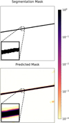 |
Fig. 3 Comparison of ground truth segmentation mask and U-Net predicted segmentation map. The top panel shows the ground truth segmentation mask with satellite trails marked in black. The bottom panel shows the U-Net predicted segmentation map, with pixel values ranging from 0 to 1, indicating the likelihood of each pixel belonging to a satellite trail. The insets provide a zoomed-in view to highlight the detailed accuracy of the predictions. |
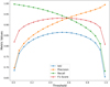 |
Fig. 4 Performance metrics for U-Net across different threshold levels: IoU, Precision, Recall, and F1-score. A threshold of 0.58 provides a balanced result in terms of all metrics tested. |
3.2 Refinement with probabilistic Hough transform
While U-Net predictions effectively identify satellite trails, they may exhibit gaps due to factors such as tumbling of the satellites, bright stars, detector defects, or unfortunate locations in the 528 × 528 pixel patches. To address these gaps in the recombined full-field binary masks, we applied a probabilistic Hough transform (Galamhos et al. 1999), which is highly effective for detecting linear patterns in images. The primary function of the Hough transform in this context is to fill in splits or gaps in the predicted trails, ensuring continuous and accurate representation. This refinement step maintains the integrity of trail detection, particularly in areas with discontinuities, and ensures more accurate statistics about satellites. This is crucial for further steps, such as estimating the total number of satellites and matching them with known satellite catalogues.
The Hough transform works by translating spatial relationships within an image into a parameter space, making it effective for detecting linear patterns like satellite trails. In this space, any line in the image can be represented as a point defined by the equation r = x cos(θ) + y sin(θ), where r is the perpendicular distance from the origin to the line, and θ is the angle of this perpendicular line with the horizontal axis. For each pixel that might belong to a satellite trail, the Hough transform evaluates every possible line through that pixel, represented by various (r, θ) combinations, resulting in a sinusoidal curve in the parameter space for each pixel. The intersection of these curves from different points indicates a consensus on the presence of a line in the image space, with accumulations in an array highlighting the most significant lines.
To address the computational intensity and scalability issues associated with the standard Hough transform, we used a probabilistic Hough transform instead. Unlike the traditional method, which examines every edge pixel in the image, the probabilistic Hough transform processes a random subset of edge points. This sampling approach significantly reduces the number of computations required, enhancing efficiency without substantially compromising detection accuracy. Additionally, the probabilistic Hough transform optimizes the resolution of the parameter space by adjusting the granularity of the (r, θ) bins. This optimization is crucial for accurately detecting satellite trails, as it balances sensitivity with computational efficiency, allowing for rapid processing of large datasets while maintaining high detection performance.
Finally, we analyzed the fraction of trails recovered by ASTA before and after applying the Hough transform using the fullfield images from our test set. Initially, ASTA had a False Negative Rate (FNR) of approximately 0.0698, meaning around 7% of a trail could be missing due to gaps caused by bright stars, artifacts, and patching required for U-Net predictions. After applying the Hough transform, the FNR was reduced by 51%, achieving an FNR of 0.0338. More importantly, trails that were previously identified as two distinct satellites were correctly reconnected into single detections. Figure 5 illustrates two cases where the U-Net prediction is improved by the Hough transform, demonstrating the process from initial detection to refined trail delineation and ensuring precise identification and continuity of satellite trails.
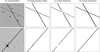 |
Fig. 5 Sequential steps of satellite trail detection and refinement: (a) Original patch image, (b) Ground truth segmentation mask, (c) U-Net predicted segmentation map, (d) Final result after applying the probabilistic Hough transform. This workflow demonstrates the process from initial detection to refined trail delineation, ensuring precise identification and continuity of satellite trails. |
3.3 Contour analysis and feature extraction
Following the refinement by the Hough transform, we obtain a binary mask consisting solely of satellite trails. The final step involves extracting features of the detected trails, such as length, width, location of start and end points, inclination, and brightness.
To achieve this, we identify the contours of the trails in the refined binary mask using the cv2.findContours function from the OpenCV package. If each satellite trail were independent, we would only need to extract the pixel values within the contour to determine the trail brightness and easily identify the most extreme points of the trail and their coordinates. However, the recent increase in satellite trails often results in multiple trails crossing each other, as shown in the first row of Fig. 5.
To address this occurrence, for each independent contour identified, there is an effective method to determine if the contour is actually the intersection of two or more trails. This is achieved by running a clustering algorithm based on DBSCAN (Density-Based Spatial Clustering of Applications with Noise, Ester et al. 1996) on the angles of the Hough transform segments that compose the current contour. This can quickly identify as many clusters as there are intersecting trails and provides an effective solution for separating them. Once the trails are separated, features such as length, width, location of start and end points, inclination, and brightness are easily extracted.
4 Application to MeerLICHT data
In this section, we applied ASTA to MeerLICHT images collected since January 2020. We analyzed approximately 200 000 non-red-flagged (i.e., science-grade) images, detecting both Low Earth Orbit (LEO) and Geostationary/Geosynchronous (GEO/GES) satellites.
Low Earth Orbit satellites typically produce streaks that span the entire field of view in a single MeerLICHT image, as illustrated in Fig. 1. While ASTA effectively detects these extensive trails, accurately identifying the specific satellites poses significant challenges. Due to their rapid movement relative to the Earth’s surface, LEO satellite trails often lack discernible start and end points within a single image. These endpoints are crucial for matching detected trails with known satellite catalogs using Two-Line Element (TLE) data, making precise identification difficult. These challenges will be addressed in a forthcoming paper. Conversely, this study focuses on the detection and identification of GEO and GES satellites, whose trails generally start and stop within the field of view during our 60-second integration time.
GEO satellites orbit Earth at an altitude of approximately 35 786 kilometers, matching the planet’s rotational period. This allows them to remain stationary relative to a fixed point on Earth. GEOs are widely used for communication, weather monitoring, and broadcasting. In astronomical images, GEOs typically appear as short streaks with a length consistent with the integration time in seconds due to the fact that the telescope tracks celestial objects and not satellites. For Meer- LICHT/BlackGEM, which use 60 s integration times, this means a streak of 15 arcminutes in length, corresponding to ~1600 pixels, in the East-West direction (90° in the convention used here).
GES satellites, on the other hand, have orbits with the same period as the Earth’s rotation but are inclined relative to the equator. This results in their position in the sky tracing an analemma over time. These satellites can appear as longer or shorter trails depending on their current position in their orbit relative to the observer and are generally at an angle to the East-West orientation on the detector.
Starting from ASTA’s results for over 200 000 MeerLICHT images, we selected all trails away from the image edges. These detected trails were then cross-referenced with satellite catalogs from celestrak.org using TLEs to ensure accurate identification. A detected trail was considered a match to a cataloged trail if the difference in their inclinations was less than 0.4 degrees, reflecting the high parallelism of well-matched trails. This 0.4-degree threshold was empirically determined based on the distribution of inclination differences between detected trails and cataloged satellite trajectories, balancing true positive matches while minimizing false positives. Additionally, the average distance between the ends of the detected and cataloged trails had to be within 200 arcseconds to account for minor timing discrepancies between observations and satellite positions.
Focusing specifically on GEO and GES satellites, we applied a declination cut between −15 and +25 degrees. We further selected detected trails with lengths between 1440 and 1640 pixels and orientations between 72.5 and 107.5 degrees, where a clear cutoff exists in the distribution of matched satellites. Out of the remaining 9107 detected trails, 7365 (80.9%) were matched to known satellites, while 1742 (19.1%) remained unmatched. Figure 6 illustrates both the matched and unmatched satellites, which form a distinct band around the projected celestial equator. Observed from South Africa, part of the Virgo galaxy cluster is projected behind the geostationary belt, resulting in a significant number of detections around Right Ascension (RA) −12 hours. These regions have been primary targets of the MeerLICHT telescope, contributing to the high concentration of detections in these areas.
Of the detected trails, 19.1% could not be matched to any objects in public catalogs. While ASTA effectively detects satellite trails, certain artifacts and image contaminations can mimic satellite signatures. However, our stringent selection criteria for angles, trail lengths, and sky coordinates significantly reduce the likelihood of such false positives. Specifically, diffraction spikes, always oriented at 45°, and linear features aligned at 0° are excluded from our search. The remaining potential artifacts, such as those caused by the saturation of bright stars (oriented at 90°), would need to coincidentally match the exact trail length range of approximately 1500 pixels to be misidentified as GEOs, which is unlikely. Figure 7 presents a pair plot of orientation angles, median brightness, and trail lengths for both matched and unmatched GEO/GES satellite trails. The diagonal panels display the marginal distributions of each quantity, while the off-diagonal panels illustrate the relationships between pairs of variables, highlighting differences between the two populations.
Visually, there are notable differences in the distribution of orientation angles and trail lengths between matched and unmatched trails. To statistically confirm these observations, we performed a consistency test (ConTEST, Stoppa et al. 2023b) comparing the distributions of orientation angles, trail lengths, and median brightness for both populations. The results indicate significant differences, leading to the rejection of the null hypothesis that the distributions are consistent. This confirms that, although matched and unmatched trails share some similarities in their properties, they belong to distinct populations.
The majority of the matched 7365 trails correspond to GEO satellites, which are characterized by their strict 90-degree orientation. In contrast, the unmatched 1742 trails exhibit a bias towards more inclined orientations. This distinction is significant for two main reasons. First, the subset of the unmatched trails that are oriented at 90 degrees are predominantly located within the geostationary belt (around +6° declination). If these 90-degree detections were artifacts of the detection method, we would expect them to be uniformly distributed across the sky. Instead, their concentration near known GEO locations indicates that they are genuine detections rather than random artifacts. Second, the inclination of the remaining unmatched trails suggests that these objects are likely Geosynchronous Transfer Orbits (GTO) satellites and older geosynchronous debris; GEOs launched decades ago tend to exhibit varying inclinations due to solilunar perturbations over the years. These inclined objects are more difficult to track and predict over time, resulting in their absence from public satellite catalogs. Consequently, the unmatched trails detected by ASTA represent genuine, albeit less-tracked, objects in Earth’s orbit. With optical telescopes like MeerLICHT and BlackGEM, we can successfully trace these inclined satellites, enhancing our ability to monitor and manage space debris.
By identifying and cataloguing these unmatched satellites, especially if they are observed in multiple images taken within a short time frame and exhibit realistic orbital characteristics, we can contribute to the maintenance and expansion of public satellite catalogues. This effort is crucial for maintaining the safety and accuracy of future astronomical observations and could aid in the management and mitigation of space debris.
 |
Fig. 6 Matched (left) and unmatched (right) GEO/GES satellite trails in celestial equatorial coordinates. The geostationary belt is visible at Dec=+6°, as observed from South Africa. The sinusoidal band are the geosynchronous satellites. The unmatched trails show satellites in both the geostationary belt and in geosynchronous orbit, as well as more extreme cases at slightly higher and lower declinations. |
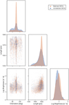 |
Fig. 7 Pair plot of orientation angles, median brightness, and trail lengths for matched and unmatched GEO/GES satellite trails. The diagonal panels show the marginal distributions of each quantity, while the off-diagonal panels display the relationships between pairs of quantities. Visually, there are significant differences in the orientation distributions of matched and unmatched trails. |
5 Conclusions
In this study, we introduced ASTA (Automated Satellite Tracking for Astronomy), a robust methodology combining U-Net and probabilistic Hough transform to detect and analyze satellite trails in ground-based astronomical observations. Using data from the MeerLICHT telescope, we demonstrated the effectiveness of ASTA in identifying and characterizing satellite trails.
Importantly, the methodology developed in this study can be easily adopted by other observatories. The use of LABKIT for manual annotation ensures a straightforward and reproducible process, encouraging other researchers and observatories to implement similar techniques. By sharing this approach, we hope to foster a collaborative effort in addressing the challenges posed by satellite trails, improving data quality across various astronomical facilities.
The U-Net’s performance was rigorously evaluated on a test set of 20 000 image patches, achieving approximately 94% precision and 94% recall. This high detection accuracy demonstrates the model’s capability in effectively identifying satellite trails amidst complex backgrounds. Furthermore, the integration of deep learning and classical image processing techniques, specifically the probabilistic Hough transform, proved effective in refining trail detection, achieving a False Negative Rate of only 3% and successfully reconnecting split trails even in the presence of bright stars and other challenging background features.
When applied to around 200 000 full-field MeerLICHT images focusing on Geostationary (GEO) and Geosynchronous (GES) satellites, ASTA matched 80.9% of the detected trails (7365 out of 9107) with known satellites in public catalogs. Additionally, ASTA identified 19.1% of trails (1742) that could not be matched to any objects in public satellite catalogs. These unmatched trails are predominantly GES, in particular Geosynchronous Transfer Orbits objects, such as rocket stages, as well as decades old geostationary satellites exhibiting varying inclinations due to solilunar perturbations. The specific orientations and concentrations of these unmatched trails further support the conclusion that they are genuine objects, highlighting ASTA’s effectiveness not only in identifying known satellites but also in uncovering new objects.
Future improvements could enhance artifact recognition and overall model performance. One key improvement is the use of better and larger GPUs, which would eliminate the need for patching. This would provide U-Net with more context from larger images and nearby sources, reducing confusion caused by small patches and minimizing gaps or inconsistencies in predictions. By processing larger portions of the image at once, U-Net can maintain context and continuity across the entire field, leading to more accurate and reliable detections. Additionally, increased computational efficiency from advanced GPUs will allow for faster processing times, making it feasible to analyze large datasets of astronomical images more efficiently.
Future work will concentrate on a comprehensive statistical analysis of the temporal and spatial components of all types of satellites, from GEOs to LEO satellites, using MeerLICHT and BlackGEM data collected over the last five years. This analysis will examine trends and patterns, improving our understanding of satellite distributions and their impact on observational data, providing a basis for developing more effective mitigation strategies.
Acknowledgements
We thank Dr Marco Langbroek for the insightful discussions on satellite trails and the various observational biases associated with them. P.J.G. is partly supported by SARChI Grant 111692 from the South African National Research Foundation. MeerLICHT is designed, built and operated by a consortium of universities and institutes, consisting of Radboud University, the University of Cape Town, the South African Astronomical Observatory, the University of Oxford, the University of Manchester and the University of Amsterdam.
Appendix A Computation time
To evaluate the efficiency of ASTA, we measured the computation time required to process a full-field MeerLICHT image, including image loading, patch creation, U-Net prediction, Hough transform application, and satellite information extraction. The tests were conducted on an Alienware Area 51M equipped with an Intel Core i9-9900K processor, 32GB DDR4/2400 RAM, and an Nvidia GeForce RTX 2080 GPU.
The processing times were measured using both CPU and GPU for each of the four stages: Preprocessing, Prediction, Hough transform, and Contour Analysis. The results are summarized in Table A.1.
Average computation time and standard deviation for each processing stage using CPU and GPU.
These results demonstrate the substantial efficiency gains achievable through GPU acceleration. The average total GPU processing time was significantly lower than the total CPU processing time, highlighting the critical role of GPU acceleration in handling large volumes of astronomical data effectively.
The Contour Analysis stage exhibits the highest variability in computation time, which can be attributed to the complexity and number of detected satellite trails in each image. The variability arises from the differing number of contours that need to be processed and the presence of intersecting trails, which require additional computation to separate accurately.
References
- Andersson, F., Carlsson, M., & Nikitin, V. V. 2016, SIAM J. Imaging Sci., 9, 637 [CrossRef] [Google Scholar]
- Arzt, M., Deschamps, J., Schmied, C., et al. 2022, Front. Comp. Sci., 4 [Google Scholar]
- Bassa, C. G., Hainaut, O. R., & Galadí-Enríquez, D. 2022, A&A, 657, A75 [NASA ADS] [CrossRef] [EDP Sciences] [Google Scholar]
- Bekteševic´, D., & Vinkovic´, D. 2017, MNRAS, 471, 2626 [CrossRef] [Google Scholar]
- Bellm, E. C., Kulkarni, S. R., Graham, M. J., et al. 2019, PASP, 131, 018002 [Google Scholar]
- Bertin, E. 2011, ASP Conf. Ser., 442, 435 [Google Scholar]
- Bertin, E., & Arnouts, S. 1996, A&AS, 117, 393 [NASA ADS] [CrossRef] [EDP Sciences] [Google Scholar]
- Bloemen, S., Groot, P., Woudt, P., et al. 2016, SPIE Conf. Ser., 9906, 990664 [NASA ADS] [Google Scholar]
- Borncamp, D., & Lian Lim, P. 2019, ASP Conf. Ser., 521, 491 [NASA ADS] [Google Scholar]
- Chambers, K. C., Magnier, E. A., Metcalfe, N., et al. 2016, arXiv e-prints [arXiv:1612.05560] [Google Scholar]
- Chatterjee, S., Kudeshia, P., Kollo, N., et al. 2024, Proceedings of the Conference on Robots and Vision, https://crv.pubpub.org/pub/4pjbqrde [Google Scholar]
- Cheselka, M. 1999, ASP Conf. Ser., 172, 349 [NASA ADS] [Google Scholar]
- Dawson, W., Schneider, M., & Kamath, C. 2016, in Advanced Maui Optical and Space Surveillance Technologies Conference, ed. S. Ryan, 72 [Google Scholar]
- Duda, R. O., & Hart, P. E. 1972, Commun. ACM, 15, 11 [CrossRef] [Google Scholar]
- Elhakiem, A. A., Ghoniemy, T. S., & Salama, G. I. 2023, J. Phys. Conf. Ser., 2616, 012024 [NASA ADS] [CrossRef] [Google Scholar]
- Ester, M., Kriegel, H.-P., Sander, J., & Xu, X. 1996, in Proceedings of the Second International Conference on Knowledge Discovery and Data Mining, KDD’96 (USA: AAAI Press), 226 [Google Scholar]
- Galamhos, C., Matas, J., & Kittler, J. 1999, Proc. IEEE Comp. Soc. Conf. Comp. Vision Pattern Recog., 1, 554 [Google Scholar]
- Gallozzi, S., Paris, D., Scardia, M., & Dubois, D. 2020, arXiv e-prints [arXiv:2003.05472] [Google Scholar]
- Groot, P. J. 2022, A&A, 667, A45 [NASA ADS] [CrossRef] [EDP Sciences] [Google Scholar]
- Groot, P. J., Bloemen, S., Vreeswijk, P. M., et al. 2024, PASP, 136, 11 [Google Scholar]
- Hainaut, O. R., & Williams, A. P. 2020, A&A, 636, A121 [EDP Sciences] [Google Scholar]
- Hosenie, Z., Bloemen, S., Groot, P., et al. 2021, Exp. Astron., 51, 319 [CrossRef] [Google Scholar]
- Ivezic´, Ž., Kahn, S. M., Tyson, J. A., et al. 2019, ApJ, 873, 111 [NASA ADS] [CrossRef] [Google Scholar]
- Kruk, S., García-Martín, P., Popescu, M., et al. 2023, Nat. Astron., 7, 262 [CrossRef] [Google Scholar]
- Lang, D., Hogg, D. W., Mierle, K., Blanton, M., & Roweis, S. 2010, AJ, 137, 1782 [NASA ADS] [CrossRef] [Google Scholar]
- LeCun, Y., Haffner, P., Bottou, L., & Bengio, Y. 1999, in Shape, Contour and Grouping in Computer Vision, eds. D. Forsyth, J. Mundy, V. di Gesu, & R. Cipolla, Lecture Notes in Computer Science, (including subseries Lecture Notes in Artificial Intelligence and Lecture Notes in Bioinformatics) (Berlin: Springer Verlag) [Google Scholar]
- Mallama, A. 2022, arXiv e-prints [arXiv:2203.05513] [Google Scholar]
- Mannor, S., Peleg, D., & Rubinstein, R. 2005, in Proceedings of the 22nd International Conference on Machine Learning, ICML ‘05 (New York, NY, USA: Association for Computing Machinery), 561 [Google Scholar]
- McDowell, J. C. 2020, ApJ, 892, L36 [Google Scholar]
- Nir, G., Zackay, B., & Ofek, E. O. 2018, AJ, 156, 229 [NASA ADS] [CrossRef] [Google Scholar]
- Paillassa, M., Bertin, E., & Bouy, H. 2020, A&A, 634, A48 [NASA ADS] [CrossRef] [EDP Sciences] [Google Scholar]
- Radon, J. 1986, IEEE Trans. Medical Imaging, 5, 170 [CrossRef] [Google Scholar]
- Ronneberger, O., Fischer, P., & Brox, T. 2015, in Medical Image Computing and Computer-Assisted Intervention – MICCAI 2015, eds. N. Navab, J. Hornegger, W. M. Wells, & A. F. Frangi (Cham: Springer International Publishing), 234 [Google Scholar]
- Stark, D. V., Grogin, N., Ryon, J., & Lucas, R. 2022, Instrum. Sci. Rep. ACS, 8, 25 [Google Scholar]
- Steeghs, D., Galloway, D. K., Ackley, K., et al. 2022, MNRAS, 511, 2405 [NASA ADS] [CrossRef] [Google Scholar]
- Stoppa, F. 2024, Dataset for: ASTA (Automated Satellite Tracking for Astronomy) [Google Scholar]
- Stoppa, F., Vreeswijk, P., Bloemen, S., et al. 2022, A&A, 662, A109 [NASA ADS] [CrossRef] [EDP Sciences] [Google Scholar]
- Stoppa, F., Bhattacharyya, S., Ruiz de Austri, R., et al. 2023a, A&A, 680, A109 [NASA ADS] [CrossRef] [EDP Sciences] [Google Scholar]
- Stoppa, F., Cator, E., & Nelemans, G. 2023b, MNRAS, 524, 1061 [NASA ADS] [CrossRef] [Google Scholar]
- Stoppa, F., Ruiz de Austri, R., Vreeswijk, P., et al. 2023c, A&A, 680, A108 [NASA ADS] [CrossRef] [EDP Sciences] [Google Scholar]
- Sudre, C. H., Li, W., Vercauteren, T. K. M., Ourselin, S., & Cardoso, M. J. 2017, Deep learning in medical image analysis and multimodal learning for clinical decision support : Third International Workshop, DLMIA 2017, and 7th International Workshop, ML-CDS 2017, 240 [Google Scholar]
- Taghanaki, S. A., Zheng, Y., Kevin Zhou, S., et al. 2019, Comput. Medical Imaging Graphics, 75, 24 [CrossRef] [Google Scholar]
- Tonry, J. L., Denneau, L., Heinze, A. N., et al. 2018, PASP, 130, 064505 [Google Scholar]
- Turin, G. 1960, IRE Trans. Inform. Theory, 6, 311 [CrossRef] [Google Scholar]
- Tyson, J. A., Ivezic´, Ž., Bradshaw, A., et al. 2020, AJ, 160, 226 [NASA ADS] [CrossRef] [Google Scholar]
- Virtanen, J., Granvik, M., Torppa, J., et al. 2014, in Asteroids, Comets, Meteors 2014, eds. K. Muinonen, A. Penttilä, M. Granvik, A. Virkki, G. Fedorets, O. Wilkman, & T. Kohout, 570 [Google Scholar]
- Walker, C., Hall, J., Allen, L., et al. 2020, BAAS, 52, 0206 [Google Scholar]
- Waszczak, A., Prince, T. A., Laher, R., et al. 2017, PASP, 129, 034402 [NASA ADS] [CrossRef] [Google Scholar]
- Zackay, B., Ofek, E. O., & Gal-Yam, A. 2016, ApJ, 830, 27 [NASA ADS] [CrossRef] [Google Scholar]
- Zimmer, P., Ackermann, M., & McGraw, J. T. 2013, in Advanced Maui Optical and Space Surveillance Technologies Conference, ed. S. Ryan, E31 [Google Scholar]
All Tables
Average computation time and standard deviation for each processing stage using CPU and GPU.
All Figures
|
Fig. 1 Full-field, 10560 × 10560 pixels, MeerLICHT image with a 60- second exposure, showcasing five satellite trails overlaying dozens of sources. |
| In the text | |
|
Fig. 2 Examples of satellite trail annotations in MeerLICHT images. The figure shows two columns and four rows: (a) original images with satellite trails of varying intensities and types in the first column, (b) corresponding labeled ground truth masks in the second column. |
| In the text | |
|
Fig. 3 Comparison of ground truth segmentation mask and U-Net predicted segmentation map. The top panel shows the ground truth segmentation mask with satellite trails marked in black. The bottom panel shows the U-Net predicted segmentation map, with pixel values ranging from 0 to 1, indicating the likelihood of each pixel belonging to a satellite trail. The insets provide a zoomed-in view to highlight the detailed accuracy of the predictions. |
| In the text | |
|
Fig. 4 Performance metrics for U-Net across different threshold levels: IoU, Precision, Recall, and F1-score. A threshold of 0.58 provides a balanced result in terms of all metrics tested. |
| In the text | |
|
Fig. 5 Sequential steps of satellite trail detection and refinement: (a) Original patch image, (b) Ground truth segmentation mask, (c) U-Net predicted segmentation map, (d) Final result after applying the probabilistic Hough transform. This workflow demonstrates the process from initial detection to refined trail delineation, ensuring precise identification and continuity of satellite trails. |
| In the text | |
|
Fig. 6 Matched (left) and unmatched (right) GEO/GES satellite trails in celestial equatorial coordinates. The geostationary belt is visible at Dec=+6°, as observed from South Africa. The sinusoidal band are the geosynchronous satellites. The unmatched trails show satellites in both the geostationary belt and in geosynchronous orbit, as well as more extreme cases at slightly higher and lower declinations. |
| In the text | |
|
Fig. 7 Pair plot of orientation angles, median brightness, and trail lengths for matched and unmatched GEO/GES satellite trails. The diagonal panels show the marginal distributions of each quantity, while the off-diagonal panels display the relationships between pairs of quantities. Visually, there are significant differences in the orientation distributions of matched and unmatched trails. |
| In the text | |
Current usage metrics show cumulative count of Article Views (full-text article views including HTML views, PDF and ePub downloads, according to the available data) and Abstracts Views on Vision4Press platform.
Data correspond to usage on the plateform after 2015. The current usage metrics is available 48-96 hours after online publication and is updated daily on week days.
Initial download of the metrics may take a while.