| Issue |
A&A
Volume 694, February 2025
|
|
|---|---|---|
| Article Number | A49 | |
| Number of page(s) | 13 | |
| Section | Numerical methods and codes | |
| DOI | https://doi.org/10.1051/0004-6361/202452756 | |
| Published online | 31 January 2025 | |
A method for asteroid detection using convolutional neural networks on VST images
1
Laboratory of Astrophysics, École Polytechnique Fédérale de Lausanne,
Chemin Pegasi 51,
1290
Versoix,
Switzerland
2
European Space Agency/ESAC,
Camino Bajo del Castillo s/n,
28692
Madrid,
Spain
3
Fysikum, Stockholm University,
106 91
Stockholm,
Sweden
4
Université de Strasbourg, CNRS, Observatoire astronomique de Strasbourg, UMR 7550,
67000
Strasbourg,
France
5
European Southern Observatory,
Karl-Schwarzschild-Strasse 2,
85748
Garching bei München,
Germany
6
European Space Agency/ESRIN PDO NEO Coordination Centre,
Largo Galileo Galilei 1,
00044
Frascati, Roma,
Italy
7
European Space Agency/ESAC PDO NEO Coordination Centre,
Camino Bajo del Castillo s/n,
28692
Madrid,
Spain
8
Institut de Ciències del Cosmos, Universitat de Barcelona,
Martí i Franquès 1,
08028
Barcelona,
Spain
9
ICREA,
Pg. Lluís Companys 23,
Barcelona,
08010
Spain
10
European Space Agency/ESRIN,
Largo Galileo Galilei 1,
00044
Frascati, Roma,
Italy
11
Institute for Particle Physics and Astrophysics, ETH Zurich,
Wolfgang-Pauli-Strasse 27,
8093
Zurich,
Switzerland
12
Kapteyn Astronomical Institute, University of Groningen,
9700 AV
Groningen,
The Netherlands
13
Swiss Data Science Center and CVLab, École Polytechnique Fédérale de Lausanne,
1015
Lausanne,
Switzerland
★ Corresponding author; This email address is being protected from spambots. You need JavaScript enabled to view it.
Received:
25
October
2024
Accepted:
9
January
2025
Abstract
Context. The study of asteroids, particularly near-Earth asteroids, is key to gaining insights into our Solar System and can help prevent dangerous collisions. Beyond finding new objects, additional observations of known asteroids will improve our knowledge of their orbit.
Aims. We have developed an automated pipeline to process and search for asteroid trails in images taken with OmegaCAM, the wide- field imager mounted on the VLT Survey Telescope (VST), on the European Southern Observatory’s Cerro Paranal. The pipeline inputs a FITS image and outputs the position, length, and angle of all the asteroids trails detected.
Methods. A convolutional neural network was trained on a set of synthetic asteroid trails, with trail lengths 5–120 pixels (1–25″) and S/Ns 3–20. Its performance was tested on synthetic trails and validated using real trails, chosen from the Solar System Object Image Search of the Canadian Astronomy Data Centre.
Results. On the synthetic trails, the pipeline achieved a completeness of 70% for trails with length ≥15 pixels (3″), with a precision of 82%. On the real trails, the pipeline achieved a completeness of 65%, with a precision of 44%, a lower value likely due to the higher presence of contaminants and stars in the field. The pipeline was able to detect both low- and high-S/N asteroid trails.
Conclusions. Our method shows a strong potential to make new discoveries and precoveries in VST data across the S/N range studied, especially in the fainter end, which remains largely unexplored.
Key words: minor planets, asteroids: general
© The Authors 2025
 Open Access article, published by EDP Sciences, under the terms of the Creative Commons Attribution License (https://creativecommons.org/licenses/by/4.0), which permits unrestricted use, distribution, and reproduction in any medium, provided the original work is properly cited.
This article is published in open access under the Subscribe to Open model. This email address is being protected from spambots. You need JavaScript enabled to view it. to support open access publication.
1 Introduction
The asteroids in our neighbourhood can unveil crucial scientific insights. Rarely subject to major perturbations, but instead to gravitational and radiation-related forces, these rocky objects have remained almost unchanged since the assembly of the Solar System, 4.6 billion years ago. First, in terms of chemical composition; second, their orbital components, once solved for, show relatively constant movements over the years. As such, asteroids can provide us with a gaze into the past to characterise this formation process. For instance, the composition analysis of main-belt asteroids has yielded clues of planetary migration in the Solar System (DeMeo & Carry 2014), while trans-Neptunian objects have been used to understand the organic composition of planets (Pinilla-Alonso et al. 2024). Some asteroids can even carry information about extrasolar systems, such as the interstellar object 11/2017 U1 (‘Oumuamua), described by Meech et al. (2017). Beyond the scientific interest of asteroid accounting, there lies a societal concern. Some of these asteroids have orbits that pass close to the Earth and pose a threat of colliding with our planet. Any asteroid with an orbit within 1.3 au from the Sun is considered a near-Earth asteroid (NEA) and should thus be studied to assess the risk of collision impact. Albeit scarce, these events can release large amounts of energy and cause local and regional destruction. The most recent example of large proportions took place in 2013, when a meteor disintegrated over the Russian city of Chelyabinsk, injuring 1500 people and releasing ~500 kilotons of energy, approximately 30 times more than the Hiroshima bomb (Brown et al. 2013; Popova et al. 2013).
According to the Minor Planet Center, as of October 2024, we know of more than 36 200 NEAs1. Of these, at least 7% have a minimum orbital intersection distance and an absolute magnitude HV—which is traditionally assumed to indicate the size of the object—to be considered potentially hazardous (i.e., HV ≤ 22 mag). Recent work has waived the absolute-magnitude criterion under the assumption that it is not an accurate proxy for the size. This would raise the potentially hazardous population to at least 25% of the known NEAs (Grav et al. 2023). However, these numbers only represent a small fraction of the real population. Although more than 90% of the existent NEAs larger than 1 km have been detected, studies such as Harris & D’Abramo (2015) prove that the discovery rate falls steeply with the decrease in size, and the estimations predict that more than 99% of the total NEA population larger than 1 m across is still unknown. This size threshold corresponds to an energy release of ~20 kilotons.
To prevent and mitigate the occurrence of asteroid encounters, a comprehensive accounting of these objects must be kept. For this, dedicated planetary-defence bodies have been established, such as the Planetary Defence Office of the European Space Agency (ESA) (Koschny 2021; Fohring et al. 2023) or the NASA Planetary Defense Coordination Office (Landis & Johnson 2019), and a wide range of astronomical surveys have been used to find or characterise NEAs. Some surveys, such as Catalina (Christensen et al. 2012) or Pan-STARRS (Kaiser et al. 2002), are specifically built to detect them or track the movement of known asteroids, which, as a result, appear as point-like sources amidst a background of trailed stars. Other surveys do not do dedicated observations, and any asteroids in these images are an unsought by-product of a different scientific goal, which usually involves tracking the background stars.
In any of the cases when they are not tracked directly, and due to their high velocity with respect to the stars tracked, the asteroids appear as trails of light in these images. This is the case for the Zwicky Transient Facility (ZTF), whose exposures of 47 square degrees have been used to detect the trails left by hundreds of NEAs (Ye et al. 2019), but many other wide-field astronomical surveys can be fit for this purpose since large portions of the sky can be scanned at a time. For the present work, we have focused on the VLT Survey Telescope (VST), for which there is not yet a dedicated blind asteroid-detection pipeline. After more than 13 years of observations, the VST catalogue comprises 399 552 r-band images of the southern sky, a coverage displayed in Figure 1. The intended detections can be performed on both new images and catalogue data.
For long-exposure astronomical images, blind asteroid searching implies a quest for extended trails of light. Their length in pixels displayed in the image will be a function of the exposure time, the angular velocity of the asteroid, and the pixel size of the camera. In addition, the appearance of the trail will be affected by the brightness of the asteroid and any possible rotation or tumbling, which may cause brightness variations along the trail (Pravec et al. 2002). Figure 2 shows the appearance of different asteroid trails with different signal-to-noise ratios (S/Ns) and trail lengths, with the values predicted using the JPL Horizons System2 (Giorgini 2015).
The trails left by asteroids have to be discerned from other elongated features usually present in the images, either physical objects–such as edge-on galaxies or satellites–or optical artefacts–such as diffraction spikes caused by bright stars or columns of dead pixels in the CCDs. Several examples of these misleading features are shown in Figure 3. Although traditional line-detection methods, such as the Hough transform (Duda & Hart 1972) or the Radon transform (Helgason & Helgason 1980; Nir et al. 2018), can be optimised to find linear objects in the images, on single exposures they fail to tell apart different objects of similar size. For instance, diffraction spikes and edge-on galaxies can have similar lengths to those of asteroid trails. As a consequence, these approaches usually rely on repeated observations to cross-match between images (Lo et al. 2019) or on manual verification, such as the work presented by Bouquillon & Souami (2020), which detected main-belt asteroids in near opposition in the Ground Based Optical Tracking of the Gaia satellite (VST).
Other classical approaches include the well-established segmentation software SourceExtractor (Bertin & Arnouts 1996), which, in this case, cannot be used either to directly produce asteroid catalogues since it does not perform well with very elongated sources, such as asteroid trails. Again, previous work has relied on multiple observations of the same field (dithers) and compared several source catalogues to conclusively identify the presence of asteroid trails, such as the method presented by Mahlke et al. (2018) for the Kilo Degree Survey (VST). On the other hand, algorithms for space-debris or satellite detection that search for very long trails, such as the spatial-filter approach by Vananti et al. (2020), are not appropriate for the short trails left by asteroids.
Within the classical approaches, perhaps the most popular algorithm for this task is StreakDet, funded by ESA and widely applied to trail detection (Virtanen et al. 2014). This software performs image segmentation, classifies the objects present in an image, and characterises their physical features. Saifollahi et al. (2023) developed a precovery pipeline for scanning the whole VST archive starting from a catalogue of known objects and their orbital parameters. Their work curated a list of VST frames using the Solar System Object Image Search3 (SSOIS) of the Canadian Astronomy Data Centre (Gwyn et al. 2015) that were predicted to contain asteroid appearances and used StreakDet to analyse them. However, their use of StreakDet reported a high number of false positives and problems when applied to long trails.
For handling complex contexts of trail detection, machine-learning algorithms–particularly convolutional neural networks–have outperformed traditional methods and are faster for processing large amounts of data. This ability is essential for the upcoming surge of astronomical surveys, such as the Large Synoptic Survey Telescope (Ivezić et al. 2019), which will generate millions of images that will need fast and effective processing. In this direction, the software MAXIMASK (Paillassa et al. 2020) performs a quick search for ‘image contaminants’, including trails of light that correspond to satellites. However, it has not been trained to find those left by asteroids, which are much shorter due to their lower angular velocity. For asteroid detection in particular, several machine-learning pipelines have been developed for specific survey data with remarkable performances, such as DeepStreaks (Duev et al. 2019), which searches for asteroids in ZTF difference images, and those presented by Lieu et al. (2019) and Pöntinen et al. (2023) for simulated Euclid images; the latter beating their own previous approach using StreakDet (Pöntinen et al. 2020). The Hubble Asteroid Hunter, developed by Kruk et al. (2022), shows good results for trail searching in images taken with the Hubble Space Telescope (HST); it should be noted that the asteroid trails in these images are much more affected by the relative motion of the telescope around the Earth, and thus appear slightly curved instead of straight.
However, none of these networks is both specifically tailored to images taken with the VST and capable of blind discovery on single exposures without relying on multiple observations or known asteroid catalogues. The current paper describes a method that fills the gap within the ensemble of the algorithms discussed since it simultaneously 1) is adapted to work on VST images and 2) shows a high performance rate compared to other state-of-the-art methods. This description is structured in four parts. Section 2 defines the theoretical fundamentals of image segmentation using neural networks and delves into the specific convolutional neural network chosen for this work. Section 3 recounts the methodology used, including the choice of data, the structure of the pipeline, and the criteria to test its performance. Section 4 lays out and makes a critical analysis of the results of this test and compares them to those reported in the previous literature. Lastly, Section 5 summarises the main conclusions of this work and outlines the next steps to improve it.
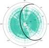 |
Fig. 1 Sky coverage of the VST catalogue in the r-band, comprising 399 552 observations as of 28 September 2024. The galactic plane is illustrated with a black line. Adapted from Saifollahi et al. (2023). |
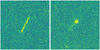 |
Fig. 2 Examples of real asteroid trails visible in images taken with the VST, at an altitude of 2635 m. Panel a: S/N of 10.1, length of 49 pixels, altitude above the horizon of 68°, and exposure time of 45 s. Panel b: S/N of 3.5, length of 28 pixels, altitude above the horizon of 60°, and exposure time of 360 s; the smeared-out appearance of the trail is due to its very low S/N, which makes it difficult to distinguish from the background noise. The S/N quoted is per pixel. |
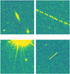 |
Fig. 3 Common linear features that can be mistaken for asteroid trails in images taken with the VST, at an altitude of 2635 m: edge-on galaxies (a), satellites (b), diffraction spikes (c), and cosmic rays (d). All images were taken with an exposure time of 360 s and a seeing of ≈0.6″. The altitude above the horizon was 71° for panels a, c and d, and 56° for panel b. |
2 Image segmentation using CNNs
2.1 Convolutional neural networks
Neural networks are deep-learning algorithms (or ‘models’), a subset of machine learning that uses layers of computing units, known as nodes, to perform a specific task. This is achieved through a process called ‘training’, where the model iteratively adjusts the weights of the nodes to optimise its performance. More specifically, convolutional neural networks (CNNs) use layers containing filters that perform a range of transformations on spatial data, mainly images. In this development, which occurs during the training, the CNN is fed with example images and learns to detect certain features or patterns. After this process, the network becomes able to generalise to and process unseen images.
The first CNN was developed by LeCun et al. (1998) for handwritten number recognition, and, since then, CNN models have evolved to cater for applications in a wide variety of contexts, including, for instance, medical imaging or climate monitoring (Anwar et al. 2018; Liu et al. 2016). In astronomy, CNNs have been used, for instance, to extract features from galaxy images for morphological classification (Cheng et al. 2020), classify stellar spectra (Sharma et al. 2019), map X-ray variability in black holes (Ricketts et al. 2023), analyse light curves for exoplanet detection (Shallue & Vanderburg 2018), or detect galaxy-scale gravitational lenses (Schaefer et al. 2018).
In this context, image segmentation is the operation by which a CNN screens an image and establishes regions of interest, assigning them specific labels. This method is more sophisticated than simple object detection, which retrieves spatial information only to a certain degree of resolution. Figure 4 illustrates the output expected from each of the two methods: in the case of simple object detection, the algorithm yields a bounding box around the object; in the case of image segmentation, the algorithm yields a pixel-wise resolution map where the object of interest is spatially defined.
A review of several image-segmentation CNNs for streak detection can be found in Fraser (2025). One of the most popular architectures is U-Net, which was initially developed for biomedical imaging and follows an encoder-decoder structure (Ronneberger et al. 2015): the encoder part aims to apply filters to extract key features from an image, while the decoder uses the extracted features to build the segmented representation of the image. U-Nets have been successfully used for streak detection in astronomical images, for instance, in Jeffries & Acuña (2024) and in Stoppa et al. (2024).
 |
Fig. 4 Comparison of two different CNN detection outputs. Panel a shows the more basic object detection, which places a bounding box around the area of interest, and panel b shows image segmentation, which produces a detailed location map of the object. Personal image taken with the TELESTO telescope (University of Geneva). |
2.2 TernausNet
The experiments in this work are done using the TernausNet architecture in the implementation4 presented by Pantoja-Rosero et al. (2022). TernausNet was originally described by Iglovikov & Shvets (2018) and evolves from the U-Net architecture by including an additional block present in the encoder that is pretrained on an image bank, ImageNet (Russakovsky et al. 2015). This choice responds to the fact that the pre-trained block is shown to speed up the convergence of the training, even if the images the model will be trained with are not directly related to those on ImageNet. This feature produces accurate predictions and improves the robustness of TernausNet with respect to U-Net in cases where the training dataset is relatively small. Furthermore, TernausNet has been proven to excel in detecting linear features, as discussed in Pantoja-Rosero et al. (2022), who applied it to detect cracks in buildings left by earthquakes.
Specifically, at each layer of the encoder, the size of the input image is reduced, while the number of channels–maps of recognisable features–is increased. As a result, the model is progressively more able to extract complex features after each stage of the encoder. In the decoder, the feature maps are upsampled again to achieve their original resolution, creating a segmentation mask that can be used to predict the class of each pixel in the input image. Figure 5 depicts a schematic of the architecture, where each block represents the characteristics of the data after each layer of transformations. The thickness of the blocks relates to the number of channels of the data, a value that increases throughout the encoder and decreases throughout the decoder, while the height of the blocks relates to the relative map size of the data and follows the inverse procedure.
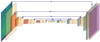 |
Fig. 5 Schematic of the TernausNet architecture and the transformations performed on the input image (left). Yellow blocks represent convolutions and transpose convolutions, while red and blue blocks depict max-pooling and unpooling, respectively. The arrows from the encoder (first half) to the decoder (second half) show skip connections, which connect non-adjacent layers and enhance the performance of the network. The thickness of the blocks is proportional to the number of channels after the transformation; the input image has three (RGB) and the sigmoid output has one. The height of the blocks relates to the relative map size after the transformation. Adapted from Iglovikov & Shvets (2018). |
2.3 MSE loss
To improve the performance of the neural network, the operation of passing the data through the encoder-decoder channel is done iteratively, testing for different model parameters that minimise a set mathematical function, the loss, which can be based on either pixel classification or distance regression. Pixel-classification losses consider the accuracy of the model when labelling each pixel, which implies that for images containing a low proportion of pixels belonging to the class of interest, the information per image that can be used for training is scarce. On the other hand, distance-regression losses assess the ability of the model to classify the distance from each pixel to the nearest object of interest, thus extracting much more information from those training images that contain few relevant pixels or whose annotations are inexact. Within the latter group, the mean-squared-error loss (LMSE) is a robust and widespread choice. It uses the squared distance between the ground truth and the prediction, averaged by the whole input. Mathematically, as described in Pantoja-Rosero et al. (2022), for an image I comprised by pixels p, it can be expressed as follows:
![Mathematical equation: ${L_{{\rm{MSE}}}}\left( {{y_d},{{\hat y}_d}} \right) = \mathop \sum \limits_{p \in I} {\left( {{y_d}[p] - {{\hat y}_d}[p]} \right)^2},$](/articles/aa/full_html/2025/02/aa52756-24/aa52756-24-eq1.png) (1)
(1)
where yd is the distance map predicted by the neural network and ŷd is the ground-truth distance map.
Given the small proportion of pixels covered by asteroids in astronomical images–with respect to those depicting the background sky, the stars or image artefacts–LMSE was chosen for the training process.
3 Methodology
3.1 Synthetic dataset
The dataset used for this study was comprised of images taken with OmegaCAM, a visible-light camera mounted on the VST, while it was operated by the European Southern Observatory (ESO) (Kuijken et al. 2002). This camera has a spatial resolution of 0.21″ per pixel and contains a mosaic of 32 CCDs, each with size 2144 × 4200 pixels, an arrangement encompassing approximately 256 million pixels. The dataset used for training and testing the algorithm was made of individual CCD frames taken in the context of the ERC COSMICLENS (PI: F. Courbin) and part of the data used in the TDCOSMO collaboration to measure time delays in lensed quasars, each with an exposure time of 320 s. The survey takes four consecutive images in the r band of each field every night, but for this work, the individual exposures were treated independently and not stacked. The selected images for the synthetic dataset were chosen at random from several different fields, but all at an absolute galactic latitude of ≥35° to reduce the number of stars crowding the field. All images had undergone a basic calibration process by the TDCOSMO collaboration that included flatfielding and bias and dark correction.
To ensure the traceability of the results, a synthetic asteroid population was injected into these images. On average, 15 asteroids were added to each CCD frame. The asteroids were represented as light trails of random lengths from 5 to 120 pixels to depict the range of sky motions from 5″/h to 2°/h. We should note that the definition of S/N used hereafter assumes that the signal is in a one-dimensional trail of width 1 pixel, but after convolution, this theoretical value is spread over several pixels in the transverse direction, and the trail appears dimmer in practice. The brightness of the synthetic asteroids was adjusted to fulfil an S/N between 3 and 20, with a distribution such that there were twice as many asteroids with S/N between 3 and 10 as there were in the rest of the interval. This choice aimed to artificially increase the attention of the network towards the asteroids in the fainter end of the range since they are the most difficult to detect. The brightness of the asteroids was determined by calculating the flux needed to obtain a specific S/N per pixel, distributing such a flux along the trail, and then convolving it with the point-spread function (PSF). To ensure that the result was as realistic as possible, the width of the PSF of each frame was estimated by identifying all stars in a given image using SourceExtractor and measuring their full width at half maximum (FWHM). This value was used for building the convolutional kernel with the Astropy function Gaussian2DKernel, which applies a Gaussian filter to generate a normalised kernel. In this case, the simulated asteroid population was not intended as an accurate depiction of the distribution of a natural asteroid population but rather as a tool to measure the potential of our algorithm. Consequently, the asteroids were located at random locations and orientations within the image. Since the rotation rates of asteroids of this size are usually at least one order of magnitude larger than the exposure time of the VST frames, any light variation stemming from asteroid rotation was not represented.
The CCD images were converted from Flexible Image Transport System (FITS) to Portable Network Graphic (PNG), the format with which TernausNet was optimised to work. To normalise the images, Astropy’s ZScaleInterval was used, an interval specifically designed to enhance values near the median of the image while decreasing the impact of outliers. All default values of the interval were applied except for the scaling factor, which was set to 0.5, the value that experimentally showed to facilitate the detection of faint asteroids. The images were further divided into smaller cutouts of size 256 × 256 pixels to ease their processing and split into a training dataset of 20 352 cutouts and a validation dataset of 5248 cutouts, which was used for assessing the algorithm during the training without affecting the training process itself.
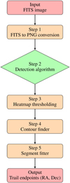 |
Fig. 6 Structure of the detection pipeline, which takes as input an image in FITS format and outputs the endpoint positions in RA, Dec of the asteroid trails found. |
3.2 Model training and pipeline description
As discussed, during the training, the model progressively adjusts its parameters to achieve the optimal configuration for the task. However, there are certain variables, known as ‘hyper-parameters’, that are fixed before the training and affect its performance. Their value is decided upon experimentally. In this work, two hyperparameters were tested: the learning rate of the model, which determines the step size per iteration at which the model moves towards the loss minimum, and the batch size, which controls the number of examples reviewed by the model before each time the parameters are adjusted. Six models were trained, each with a different learning rate (5 × 10⁻⁶ and 5 × 10⁻⁷) and a different batch size (16, 32, and 64), for a total of 100 iterations.
The best configuration of the hyperparameters would be used for the detection algorithm, the first of the five stages of the pipeline, to which the full CCD images are fed. A schematic of the pipeline can be found in Figure 6. For computational efficiency, the algorithm divides the images into 1024 × 1024 patches to perform the detection process on each of the individual tiles, a larger size than for training since testing is less computationally intensive. Padding is applied whenever the patch cut lies outside the limits of the image. After the detection algorithm is executed, the results are again reassembled to the original image size. The output of this first stage is a probability heatmap representing the most likely distance to the nearest asteroid trail, as seen in Figure 7. More specifically, each pixel is colour-coded so that the closer it is thought to be to the centre of an asteroid trail, the darker it will appear.
Since the heatmap shows probability distributions rather than discrete labels of whether a pixel belongs to a trail or not, a thresholding step is introduced to compose a binary map showing a concrete number of detections. As depicted in Figure 8, every probability pixel with a value equal to or lower than the threshold value is converted to white in the binary image, whereas every pixel below the threshold is converted to black. This threshold will influence the number of detections: on the one hand, a stricter thresholding criterion will lead to fewer detections but will also yield fewer false positives; on the other hand, a more lenient criterion will make the pipeline able to find more trails, at the cost of more false positives. The threshold is determined experimentally.
Although spatial information is used by the algorithm for creating the heatmap, the output is at a pixel level, which implies that the algorithm does not gather conclusive information on how many trails are detected or their exact location. For this, the OpenCV function findContours is used for detecting and storing the positions of any contours present within the binary image. To extract the endpoint positions from the contours, a line is fit through each contour of the binary image and the points of intersection between the lines and the contours are taken as the two preliminary endpoint values.
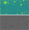 |
Fig. 7 Comparison between the original input image (above) and the detection heatmap (below) for an example CCD file. The asteroid trails displayed are synthetic. |
 |
Fig. 8 Real asteroid trail as seen in the original image, the detection heatmap, and the thresholded binary map (thresholded at 20). The asteroid trail displayed is from a real asteroid. |
3.3 Trail fitting
Given the importance of accurately determining the position of the trail for astrometry purposes, an additional step is introduced to refine the endpoint positions found using the linear fit. For this, the preliminary endpoint positions are used as initial values for a Markov Chain Monte Carlo fitting routine of 5000 walkers on the original FITS file, using the approach described in Hogg & Foreman-Mackey (2018). The list of trails found is compared with the ground truth and two trails are considered a match if the difference between their midpoint coordinates is strictly less than 15 pixels, approximately twice the average seeing.
3.4 Performance metrics
The performance of the algorithm was tested on a controlled set of 6688 synthetic asteroids, scattered over 449 CCD frames. The frames were visually inspected to confirm that no asteroid was already present in them. To test for the optimal hyperparameter configuration, the LMSE was compared for the six combinations of the different batch sizes and learning rates. Three main indicators were considered to assess the detection perfection itself: precision, completeness, and F1.
Precision, also known as purity, yields a measure of the sensitivity of the model. It is defined as
 (2)
(2)Completeness, also known as recall, indicates how exhaustive the detections are with respect to the ground-truth population sample. It is defined as
 (3)
(3)F1 score expresses a balance between precision and completeness. Since it combines these two parameters, it was used to experimentally determine the optimal thresholding value for creating the binary images. The F1 score is defined as
 (4)
(4)
In addition, we should account for the fact that the VST frames are direct science exposures and thus have objects, such as stars and galaxies, that could be covering the asteroid trails. To quantify more precisely the magnitude of the occlusion, catalogues of objects were made with SourceExtractor that included the size of the objects found. The fraction of the sky covered by these objects (non-asteroid coverage) was calculated across the test set.
3.5 Application to real asteroid data
To test the performance of the algorithm in a real environment and to verify the validity of the results in the synthetic set, a new dataset was crafted using real asteroid trails. To this end, the asteroid list used by Saifollahi et al. (2023) and extracted from the JPL Horizons System was filtered to retrieve suitable candidates. This was combined with information from the SSOIS, which retrieved all OmegaCAM frames in which the asteroids were predicted to appear. A sample in the r-band of 276 asteroid appearances with S/Ns 3–20 and trail lengths 5–120 pixels (1–25″) was taken to build a test set with similar characteristics to those of the training set.
The algorithm was applied to the new dataset, and since, as discussed in Saifollahi et al. (2023), the predicted S/Ns and asteroid positions could contain inaccuracies, all detections were visually inspected and confirmed.
4 Results and discussion
In this section, we lay out three sets of results: those resulting from the pipeline optimisation process, those resulting from applying the pipeline to test synthetic trails and those resulting from applying the pipeline to test real asteroid trails.
4.1 Results of pipeline optimisation
To identify the optimal hyperparameters for this specific model and task, the loss function LMSE was evaluated for the six models, resulting from the combination of the three batch sizes (16, 32 and 64) and the two learning rates (5 × 10⁻⁶ and 5 × 10⁻⁷). As displayed in Figure 9, the model with batch size 64 and learning rate 5 × 10⁻⁶ showed a smaller loss than the other combinations early on in the training process. Such a loss decreased throughout the training up until epoch 80, after which, albeit the training loss continued decreasing, the validation loss remained stalled. For this reason, the training was discontinued after epoch 100. The model of batch size 64 and learning rate 5 × 10⁻⁶ was chosen for all subsequent applications.
For choosing the most appropriate thresholding value to binarise the probability map produced by the model, the F1 scores at different thresholds were evaluated, as shown in Figure 10. The pixel threshold value that maximised the F1 score was found to be 20, after which the score decreased, most likely due to a rapid increase in the number of false positives reported. Hence, when creating the binary images, any values lower (darker) than 20 were set to white and any values higher than 20, to black. This ensured that the balance between false negatives and false positives was optimal.
4.2 Results on synthetic trails
The pipeline was tested on a set of 6688 asteroids with the same distributions as the training and validation datasets regarding S/N and length of trail. The test set was imbalanced in the same manner as the training dataset and contained twice as many asteroids in the S/N range 3–10 as in the range 10–20. The aim of this asymmetry was to better assess the performance within the fainter range, which presents a more challenging detectability. Hence, two-thirds of the test set were contained within this range. The completeness achieved as a function of these two variables is shown as a heatmap in Figure 11, with dark navy indicating that all asteroids within that bin were found. No asteroids with trail length below 10 pixels (2″) were found by the pipeline, and the completeness for trail length 10–20 pixels (2–4″) was also deficient across all S/Ns. The inadequate performance of the algorithm when identifying short trails was influenced by two factors. First, the short trails are often indistinguishable from other astronomical objects present in the image. Second, the detection of short trails is disproportionately affected by the presence of other objects in the field. The percentage of the image covered by stars and galaxies per frame was computed for all 449 test frames, which yielded an average of 1037 objects per frame covering 1.85% of pixels. These objects occlude the short trails and can hinder their detection more than for the case of long trails, which can still be recognisable as trails even when partially occluded. The completeness for very faint trails of S/N 3–4 is also very low for short-to-medium trails (≤50 pixels or 10.5″), although it increases for longer trails as the elongated features become more recognisable for the model, even if dim. However, these values improve significantly for brighter trails and overall, the completeness achieved by the model reached 63% for all trails and 70% for trails with length ≥15 pixels (≥3″). Given the high seeing of many of the frames, visual inspection showed that the very short trails were indistinguishable from other objects, particularly bright stars. Subdividing further in S/N, the model achieved a completeness of 33.4% for S/N 3–5, 68.8% for S/N 5–10, and 73.9% for S/N 10–20.
Since most frames used for testing had similar seeing values, the influence of the seeing could not be assessed in detail. However, the asteroids that were not detected were in frames with a slightly higher seeing, as shown in Figure 12.
In addition to the true positives, the algorithm detected 709 false positives. Upon visual inspection, 14% of these detections were caused by satellite trails, while the rest resulted either from the incorrect breakage of a single trail into two different detections–which would have also affected the completeness from the previous step–or the incorrect detection of a diffraction spike from a bright start, for most cases, as well as other linear features in the image.
The exact position of the trail is essential to determine the astrometry of the asteroid and, hence, is an essential requirement for submitting any detections to the Minor Planet Center. The results of the endpoint-fitting routine showed that the trail modelling was very accurate for all cases where the trail was clearly visible (Figure 13) and showed higher residuals whenever there was another object in the frame (Figure 14) or the trail was very faint to the eye (Figure 15).
Figure 16 displays the one- and two-dimensional projections of the posterior probability distributions of the parameters fitted in Figure 13. As described in Hogg & Foreman-Mackey (2018), these projections depict the covariance between parameters.
The accuracy of the current method was further quantified by measuring the difference in midpoint position, trail orientation angle with respect to the x-axis, and length of trail between the ground truth and the values determined by the pipeline. The results are displayed in Figures 17–19. The error in the midpoint position was, on average, 2.9 pixels (0.61″), which can be further broken down in the direction along the trail, 2.3 pixels (0.47″), and the direction perpendicular to the trail, 1.3 pixels (0.28″). It presented a disproportionate inaccuracy for very short trails, as displayed in Figure 17. Similarly, the error in the angle measured was, on average, 2.3°. As shown in panel a of Figure 18, this uncertainty affected short trails the most.
The poorer performance for short trails when quantifying the position and angle does not have a strong effect on the determination of the length of trail, displayed in Figure 19, which depicts the error in the measured length of trail relative to the trail length; on average, 1.1%. A positive value indicates that the algorithm is overestimating the length. Although the result is higher for short trails, this is not the consequence of a worse absolute performance for short trails but rather a consequence of using relative values.
Lastly, there does not seem to be a significant S/N dependence on any of the variables considered. The uncertainty is within the same order of magnitude across all S/N values for the detected endpoint position, angle, and length of trail.
It should be noted that the fitting routine described in subsection 3.3 significantly improved the characterisation of the trails. Before the fitting, the errors in the midpoint position, the trail angle, and the trail length were 8.5 pixels, 2.6°, and 17.5%, respectively. After the fitting, these values decreased to 2.9 pixels, 2.3°, and 1.1%, respectively. The initial inaccuracy directly stemmed from the line-fitting method initially used to fit the detection contours on the PNG images. The disproportionate overestimation of the length of trail was likely introduced in the thresholding step, where many pixels adjacent to the trail but not predicted to be part of it by the algorithm were added to the trail after thresholding (see Figure 8). For this reason, applying the Markov Chain Monte Carlo fitting on the original FITS image was essential before assessing the results.
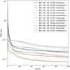 |
Fig. 9 Comparison of the MSE loss for different models throughout 100 training epochs. The model with batch size (BS) 64 and learning rate (LR) 5 × 10⁻⁶ displays the lowest values for the MSE loss, although it shows no signs of improvement after training epoch 80. |
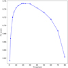 |
Fig. 10 F1 score evaluated at different thresholds before the endpoint fitting. The curve reaches a peak at threshold value 20 and swiftly decreases. |
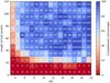 |
Fig. 11 Completeness of the algorithm applied to a test set of 6688 asteroid trails, expressed in percentage. There are ≈53 asteroids per bin in the bins with S/N 3–10 and ≈19 asteroids per bin in the bins with S/N 10–20. The minimum trail length is 5 pixels. |
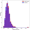 |
Fig. 12 Seeing distribution of the frames of the asteroids found vs not found. |
Comparison of the tests with the synthetic and the real asteroid trails.
4.3 Results on real trails
The results from applying the pipeline on the real asteroid trails can be seen in Figure 20, which displays the detections in terms of S/N and length of trail. As expected from the results of the synthetic test set, the performance for short trails is very poor. However, the overall completeness achieves 66%, a similar value to that of the synthetic set. As expected from the work of Saifollahi et al. (2023), visual inspection of the detections confirmed that the trail positions predicted in the catalogue could contain inaccuracies, and thus no further tests were done to assess the accuracy of the detected midpoint, length of trail and angle. Instead, given the consistency in completeness, these results were used to support the validity of the tests done with the synthetic trails.
In addition to the real asteroids, the pipeline further detected 290 objects, which implied that the precision of the pipeline when applied to real trails was 44%, a value much lower than in the synthetic dataset. Almost a third (28.5%) of the false positives were caused by satellite trails, whereas the rest were, in most cases, due to the fact that certain frames were particularly crowded, causing the false positives to spike. More precisely, the area covered by non-asteroids in this dataset was more than 2.5 times larger (4.75%) than the area in the synthetic dataset (1.85%) and was thus expected to produce a much larger number of false positives. It should also be noted that these tests were performed on raw data; hence, the precision of the method is expected to increase when applied to calibrated images, with a smaller proportion of artefacts that can mislead the algorithm. A full account of the different performance indicators for both the synthetic and the real test sets is shown in Table 1.
We envision that our method will be able to produce many more precoveries and discoveries when applied to the full VST archive. In Figure 21, the detections by our pipeline in this small subset are shown in dark blue.
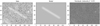 |
Fig. 13 Endpoint fitting for a normal asteroid trail of S/N 9.8. The reduced χ2 value is close to 1, which indicates that the fit is almost perfect. |
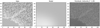 |
Fig. 14 Endpoint fitting for an asteroid trail of S/N 6.5 that is partially on a bright star. The flux of the star contaminates the model, which does not adequately capture the asteroid trail. |
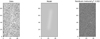 |
Fig. 15 Endpoint fitting for an asteroid trail of S/N 3.3. The model is accurate despite the faintness of the trail, but less than for the brighter cases. |
4.4 Comparison with other state-of-the-art algorithms
The results obtained by the pipeline seem robust compared to those reported in the literature. Although machine-learning pipelines for asteroid detection applied to other surveys should be compared only with the caveat of the type of data (for instance, the trails in the HST images appear more curved or the seeing in the Euclid images is much better than for VST since it is space-based), certain remarks can be made about other studies using direct single exposures. The completeness and precision achieved are higher than those reported by Kruk et al. (2022) (58.2% and 73.6%, respectively), and the precision is much higher than that reported by Pöntinen et al. (2023) (6.4% for single exposures) for a similar completeness (68.5%). Other works, such as that by Duev et al. (2019), use difference images and thus should not be compared directly. The precovery rate obtained by Saifollahi et al. (2023) of 20−50% cannot be fairly compared to the completeness presented in this work either, since it is quantifying the number of asteroids detected with respect to those predicted to be detectable. However, our algorithm does achieve a higher precision rate than the one reported for their algorithm. On individual exposures, our pipeline outperforms other algorithms when characterising the trails found with a comparable completeness. The reported average coordinate, angle, and length errors in Pöntinen et al. (2023) for Euclid images are 3.8 pixels, 1.6°, and −2.4%, respectively. In comparison, our method yields errors of 2.9 pixels, 2.3 °, and 1.1%, respectively.
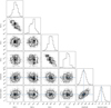 |
Fig. 16 Posterior probability distributions of the parameters fitted, including the endpoints of the trail and the characteristics of the Gaussian profile. |
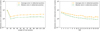 |
Fig. 17 Difference between the ground truth and the midpoint position detected by the pipeline, in pixels. Panel a shows the dependence on length of trail and panel b displays the dependence on S/N. |
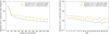 |
Fig. 18 Difference between the ground truth and the angle measured by the pipeline, in degrees. Panel a shows the dependence on length of trail and panel b displays the dependence on S/N. |
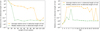 |
Fig. 19 Difference between the ground truth and the relative length of trail detected by the pipeline. This difference is calculated by dividing the error by the length of trail. Panel a shows the dependence on length of trail and panel b displays the dependence on S/N. |
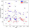 |
Fig. 20 Detection performance when applying the method to a set of 276 real trails as a function of S/N and length of trail. |
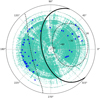 |
Fig. 21 Asteroids detected in the test (dark blue) in the context of the VST coverage in the r-band. The galactic plane is illustrated with a black line, and the dashed lines represent the ±35° distance in latitude from it. Adapted from Saifollahi et al. (2023). |
5 Conclusions and future work
A machine-learning pipeline for asteroid detection in VST images was trained using a synthetic population of NEAs. Different hyperparameters were tested to fine-tune the network, which, once trained, was applied to a test set of 6688 synthetic trails. Overall, the trained model achieved a completeness of 63% and a precision of 82%, but the results were heavily influenced by the length of the asteroid trails. For trails with lengths ≥15 pixels, the completeness was 70%, whereas no trails below 10 pixels were found. The S/N dependence was much weaker and mainly affected trails with S/N ≤ 4, with otherwise consistently good results generally across the S/N range of 4–20. To validate the results on the synthetic set, the pipeline was applied to a set of real asteroid trails and achieved a completeness of 65% and a precision of 44%. The low precision obtained in the second set, which was comprised of raw images instead of calibrated images, was likely due to the presence of several frames particularly crowded with background objects that concentrated most of the false positives and is expected to increase significantly when working on less crowded fields. Accounting for this, the overall consistency between the two test sets suggests that the synthetic set was robust. Furthermore, the definition of S/N quoted is conservative in a practical sense, which implies that in reality the algorithm could be able to find streaks even fainter than S/N 3.
The method showed a strong detection performance compared to other state-of-the-art algorithms in terms of completeness, precision, and trail characterisation. For the next steps, the pipeline should be modified to extract the S/N of the asteroids detected, which would make it a useful tool to assess the accuracy of the predicted S/Ns in the JPL Horizons list.
In future work, we will focus on applying the pipeline to a larger set of the VST archive. Since the algorithm can detect asteroid trails at an S/N 3–10, which, as discussed by Saifollahi et al. (2023), remain mostly undetected in VST frames, we expect new precoveries and discoveries will be made with our approach. Any new information gathered will improve the known orbits of asteroids–and NEAs in particular–and can, in time, help us predict future dangerous asteroid collisions.
Acknowledgements
The authors would like to thank Emmanuel Bertin, Jean-Luc Starck, Maggie Lieu, Guillermo Buenadicha, Andreu Arderieu, Jorge García Condado, and the anonymous reviewer for their helpful insights. This project has received funding from the European Union’s Horizon 2020 and Horizon Europe research and innovation programmes under the Marie Skłodowska-Curie grant agreement Nos. 945363 and 101105725, and funding from the Swiss National Science Foundation and the Swiss Innovation Agency (Innosuisse) via the BRIDGE Discovery grant 40B2-0 194729. Martin Millon acknowledges support by the SNSF (Swiss National Science Foundation) through mobility grant P500PT_203114 and return CH grant P5R5PT_225598. This work used the facilities of the Canadian Astronomy Data Centre, operated by the National Research Council of Canada with the support of the Canadian Space Agency. The data analysis is based on observations collected at the European Organisation for Astronomical Research in the Southern Hemisphere mostly under ESO programmes 106.216P.002, 098.B-0775(A), 177.A-3016(D), and 60.A-9800(Q), in addition to 106 other programmes. The following software and Python libraries were used: Astropy (Astropy Collaboration 2013, 2018, 2022), Numpy (Harris et al. 2020), OpenCV (Bradski 2000), PlotNeuralNet5, Pytorch (Paszke et al. 2019), and Scipy (Virtanen et al. 2020).
References
- Anwar, S. M., Majid, M., Qayyum, A., et al. 2018, J. Med. Syst., 42, 1 [CrossRef] [Google Scholar]
- Astropy Collaboration (Robitaille, T. P., et al.) 2013, A&A, 558, A33 [NASA ADS] [CrossRef] [EDP Sciences] [Google Scholar]
- Astropy Collaboration (Price-Whelan, A. M., et al.) 2018, AJ, 156, 123 [Google Scholar]
- Astropy Collaboration (Price-Whelan, A. M., et al.) 2022, ApJ, 935, 167 [NASA ADS] [CrossRef] [Google Scholar]
- Bertin, E., & Arnouts, S. 1996, A&ASS, 117, 393 [NASA ADS] [CrossRef] [EDP Sciences] [Google Scholar]
- Bouquillon, S., & Souami, D. 2020, arXiv e-prints [arXiv:2004.09961] [Google Scholar]
- Bradski, G. 2000, The OpenCV Library, Dr. Dobb’s Journal of Software Tools, 120, 122 [Google Scholar]
- Brown, P. G., Assink, J. D., Astiz, L., et al. 2013, Nature, 503, 238 [NASA ADS] [Google Scholar]
- Cheng, T.-Y., Conselice, C. J., Aragón-Salamanca, A., et al. 2020, MNRAS, 493, 4209 [Google Scholar]
- Christensen, E., Larson, S., Boattini, A., et al. 2012, in AAS/Division for Planetary Sciences Meeting Abstracts, 44, 210 [Google Scholar]
- DeMeo, F. E., & Carry, B. 2014, Nature, 505, 629 [NASA ADS] [CrossRef] [Google Scholar]
- Duda, R. O., & Hart, P. E. 1972, Commun. ACM, 15, 11 [CrossRef] [Google Scholar]
- Duev, D. A., Mahabal, A., Ye, Q., et al. 2019, MNRAS, 486, 4158 [NASA ADS] [CrossRef] [Google Scholar]
- Fohring, D., Conversi, L., Micheli, M., Kresken, R., & Ocana, F. 2023, LPI Contrib., 2851, 2285 [NASA ADS] [Google Scholar]
- Fraser, W. C. 2025, in Machine Learning for Small Bodies in the Solar System (Elsevier), 229 [CrossRef] [Google Scholar]
- Giorgini, J. D. 2015, in IAU General Assembly, 29, 2256293 [Google Scholar]
- Grav, T., Mainzer, A. K., Masiero, J. R., et al. 2023, Planet. Sci. J., 4, 228 [NASA ADS] [CrossRef] [Google Scholar]
- Gwyn, S. D., Hill, N., & Kavelaars, J. 2015, Proc. Int. Astron. Union, 10, 270 [CrossRef] [Google Scholar]
- Harris, A. W., & D’Abramo, G. 2015, Icarus, 257, 302 [NASA ADS] [CrossRef] [Google Scholar]
- Harris, C. R., Millman, K. J., van der Walt, S. J., et al. 2020, Nature, 585, 357 [NASA ADS] [CrossRef] [Google Scholar]
- Helgason, S., & Helgason, S. 1980, The Radon Transform, 2 (Springer) [CrossRef] [Google Scholar]
- Hogg, D. W., & Foreman-Mackey, D. 2018, ApJS, 236, 11 [NASA ADS] [CrossRef] [Google Scholar]
- Iglovikov, V., & Shvets, A. 2018, arXiv e-prints [arXiv:1801.05746] [Google Scholar]
- Ivezić, Ž., Kahn, S. M., Tyson, J. A., et al. 2019, ApJ, 873, 111 [Google Scholar]
- Jeffries, C., & Acuña, R. 2024, J. Artif. Intell. Technol., 4, 1 [Google Scholar]
- Kaiser, N., Aussel, H., Burke, B. E., et al. 2002, in Survey and Other Telescope Technologies and Discoveries, 4836, SPIE, 154 [Google Scholar]
- Koschny, D. 2021, in Legal Aspects of Planetary Defence (Brill Nijhoff), 86 [CrossRef] [Google Scholar]
- Kruk, S., Martín, P. G., Popescu, M., et al. 2022, A&A, 661, A85 [NASA ADS] [CrossRef] [EDP Sciences] [Google Scholar]
- Kuijken, K., Bender, R., Cappellaro, E., et al. 2002, The Messenger, 110, 15 [NASA ADS] [Google Scholar]
- Landis, R., & Johnson, L. 2019, Acta Astron., 156, 394 [NASA ADS] [CrossRef] [Google Scholar]
- LeCun, Y., Bottou, L., Bengio, Y., & Haffner, P. 1998, Proc. IEEE, 86, 2278 [Google Scholar]
- Lieu, M., Conversi, L., Altieri, B., & Carry, B. 2019, MNRAS, 485, 5831 [NASA ADS] [CrossRef] [Google Scholar]
- Liu, Y., Racah, E., Correa, J., et al. 2016, arXiv e-prints [arXiv:1605.01156] [Google Scholar]
- Lo, K.-J., Chang, C.-K., Lin, H.-W., et al. 2019, AJ, 159, 25 [CrossRef] [Google Scholar]
- Mahlke, M., Bouy, H., Altieri, B., et al. 2018, A&A, 610, A21 [NASA ADS] [CrossRef] [EDP Sciences] [Google Scholar]
- Meech, K. J., Weryk, R., Micheli, M., et al. 2017, Nature, 552, 378 [Google Scholar]
- Nir, G., Zackay, B., & Ofek, E. O. 2018, AJ, 156, 229 [NASA ADS] [CrossRef] [Google Scholar]
- Paillassa, M., Bertin, E., & Bouy, H. 2020, A&A, 634, A48 [NASA ADS] [CrossRef] [EDP Sciences] [Google Scholar]
- Pantoja-Rosero, B. G., Oner, D., Kozinski, M., et al. 2022, Construct. Build. Mater., 344, 128264 [CrossRef] [Google Scholar]
- Paszke, A., Gross, S., Massa, F., et al. 2019, Adv. Neural Inform. Process. Syst., 32 [Google Scholar]
- Pinilla-Alonso, N., Brunetto, R., De Prá, M. N., et al. 2024, Nat. Astron., https://doi.org/10.1038/s41550-024-02433-2 [Google Scholar]
- Pöntinen, M., Granvik, M., Nucita, A., et al. 2020, A&A, 644, A35 [NASA ADS] [CrossRef] [EDP Sciences] [Google Scholar]
- Pöntinen, M., Granvik, M., Nucita, A. A., et al. 2023, A&A, 679, A135 [NASA ADS] [CrossRef] [EDP Sciences] [Google Scholar]
- Popova, O. P., Jenniskens, P., Emel’yanenko, V., et al. 2013, Science, 342, 1069 [NASA ADS] [CrossRef] [Google Scholar]
- Pravec, P., Harris, A. W., & Michalowski, T. 2002, Asteroids III, 113, 35 [Google Scholar]
- Ricketts, B. J., Steiner, J. F., Garraffo, C., Remillard, R. A., & Huppenkothen, D. 2023, MNRAS, 523, 1946 [NASA ADS] [CrossRef] [Google Scholar]
- Ronneberger, O., Fischer, P., & Brox, T. 2015, in Medical Image Computing and computer-assisted Intervention–MICCAI 2015: 18th International Conference, Munich, Germany, October 5–9, 2015, proceedings, part III 18 (Springer), 234 [Google Scholar]
- Russakovsky, O., Deng, J., Su, H., et al. 2015, Int. J. Comput. Vis., 115, 211 [Google Scholar]
- Saifollahi, T., Kleijn, G. V., Williams, R., et al. 2023, A&A, 673, A93 [NASA ADS] [CrossRef] [EDP Sciences] [Google Scholar]
- Schaefer, C., Geiger, M., Kuntzer, T., & Kneib, J.-P. 2018, A&A, 611, A2 [NASA ADS] [CrossRef] [EDP Sciences] [Google Scholar]
- Shallue, C. J., & Vanderburg, A. 2018, AJ, 155, 94 [NASA ADS] [CrossRef] [Google Scholar]
- Sharma, K., Kembhavi, A., Kembhavi, A., et al. 2019, MNRAS, 491, 2280 [Google Scholar]
- Stoppa, F., Groot, P., Stuik, R., et al. 2024, A&A, 692, A199 [NASA ADS] [CrossRef] [EDP Sciences] [Google Scholar]
- Vananti, A., Schild, K., & Schildknecht, T. 2020, Adv. Space Res., 65, 364 [NASA ADS] [CrossRef] [Google Scholar]
- Virtanen, J., Flohrer, T., Muinonen, K., et al. 2014, 40th COSPAR Scientific Assembly, 40, PEDAS [Google Scholar]
- Virtanen, P., Gommers, R., Oliphant, T. E., et al. 2020, Nat. Methods, 17, 261 [Google Scholar]
- Ye, Q., Masci, F. J., Lin, H. W., et al. 2019, PASP, 131, 078002 [NASA ADS] [CrossRef] [Google Scholar]
All Tables
All Figures
|
Fig. 1 Sky coverage of the VST catalogue in the r-band, comprising 399 552 observations as of 28 September 2024. The galactic plane is illustrated with a black line. Adapted from Saifollahi et al. (2023). |
| In the text | |
|
Fig. 2 Examples of real asteroid trails visible in images taken with the VST, at an altitude of 2635 m. Panel a: S/N of 10.1, length of 49 pixels, altitude above the horizon of 68°, and exposure time of 45 s. Panel b: S/N of 3.5, length of 28 pixels, altitude above the horizon of 60°, and exposure time of 360 s; the smeared-out appearance of the trail is due to its very low S/N, which makes it difficult to distinguish from the background noise. The S/N quoted is per pixel. |
| In the text | |
|
Fig. 3 Common linear features that can be mistaken for asteroid trails in images taken with the VST, at an altitude of 2635 m: edge-on galaxies (a), satellites (b), diffraction spikes (c), and cosmic rays (d). All images were taken with an exposure time of 360 s and a seeing of ≈0.6″. The altitude above the horizon was 71° for panels a, c and d, and 56° for panel b. |
| In the text | |
|
Fig. 4 Comparison of two different CNN detection outputs. Panel a shows the more basic object detection, which places a bounding box around the area of interest, and panel b shows image segmentation, which produces a detailed location map of the object. Personal image taken with the TELESTO telescope (University of Geneva). |
| In the text | |
|
Fig. 5 Schematic of the TernausNet architecture and the transformations performed on the input image (left). Yellow blocks represent convolutions and transpose convolutions, while red and blue blocks depict max-pooling and unpooling, respectively. The arrows from the encoder (first half) to the decoder (second half) show skip connections, which connect non-adjacent layers and enhance the performance of the network. The thickness of the blocks is proportional to the number of channels after the transformation; the input image has three (RGB) and the sigmoid output has one. The height of the blocks relates to the relative map size after the transformation. Adapted from Iglovikov & Shvets (2018). |
| In the text | |
|
Fig. 6 Structure of the detection pipeline, which takes as input an image in FITS format and outputs the endpoint positions in RA, Dec of the asteroid trails found. |
| In the text | |
|
Fig. 7 Comparison between the original input image (above) and the detection heatmap (below) for an example CCD file. The asteroid trails displayed are synthetic. |
| In the text | |
|
Fig. 8 Real asteroid trail as seen in the original image, the detection heatmap, and the thresholded binary map (thresholded at 20). The asteroid trail displayed is from a real asteroid. |
| In the text | |
|
Fig. 9 Comparison of the MSE loss for different models throughout 100 training epochs. The model with batch size (BS) 64 and learning rate (LR) 5 × 10⁻⁶ displays the lowest values for the MSE loss, although it shows no signs of improvement after training epoch 80. |
| In the text | |
|
Fig. 10 F1 score evaluated at different thresholds before the endpoint fitting. The curve reaches a peak at threshold value 20 and swiftly decreases. |
| In the text | |
|
Fig. 11 Completeness of the algorithm applied to a test set of 6688 asteroid trails, expressed in percentage. There are ≈53 asteroids per bin in the bins with S/N 3–10 and ≈19 asteroids per bin in the bins with S/N 10–20. The minimum trail length is 5 pixels. |
| In the text | |
|
Fig. 12 Seeing distribution of the frames of the asteroids found vs not found. |
| In the text | |
|
Fig. 13 Endpoint fitting for a normal asteroid trail of S/N 9.8. The reduced χ2 value is close to 1, which indicates that the fit is almost perfect. |
| In the text | |
|
Fig. 14 Endpoint fitting for an asteroid trail of S/N 6.5 that is partially on a bright star. The flux of the star contaminates the model, which does not adequately capture the asteroid trail. |
| In the text | |
|
Fig. 15 Endpoint fitting for an asteroid trail of S/N 3.3. The model is accurate despite the faintness of the trail, but less than for the brighter cases. |
| In the text | |
|
Fig. 16 Posterior probability distributions of the parameters fitted, including the endpoints of the trail and the characteristics of the Gaussian profile. |
| In the text | |
|
Fig. 17 Difference between the ground truth and the midpoint position detected by the pipeline, in pixels. Panel a shows the dependence on length of trail and panel b displays the dependence on S/N. |
| In the text | |
|
Fig. 18 Difference between the ground truth and the angle measured by the pipeline, in degrees. Panel a shows the dependence on length of trail and panel b displays the dependence on S/N. |
| In the text | |
|
Fig. 19 Difference between the ground truth and the relative length of trail detected by the pipeline. This difference is calculated by dividing the error by the length of trail. Panel a shows the dependence on length of trail and panel b displays the dependence on S/N. |
| In the text | |
|
Fig. 20 Detection performance when applying the method to a set of 276 real trails as a function of S/N and length of trail. |
| In the text | |
|
Fig. 21 Asteroids detected in the test (dark blue) in the context of the VST coverage in the r-band. The galactic plane is illustrated with a black line, and the dashed lines represent the ±35° distance in latitude from it. Adapted from Saifollahi et al. (2023). |
| In the text | |
Current usage metrics show cumulative count of Article Views (full-text article views including HTML views, PDF and ePub downloads, according to the available data) and Abstracts Views on Vision4Press platform.
Data correspond to usage on the plateform after 2015. The current usage metrics is available 48-96 hours after online publication and is updated daily on week days.
Initial download of the metrics may take a while.