| Issue |
A&A
Volume 692, December 2024
|
|
|---|---|---|
| Article Number | A125 | |
| Number of page(s) | 18 | |
| Section | Extragalactic astronomy | |
| DOI | https://doi.org/10.1051/0004-6361/202451482 | |
| Published online | 05 December 2024 | |
CO-CAVITY project: Molecular gas and star formation in void galaxies
1
Departamento de Física Téorica y del Cosmos, Universidad de Granada, 18071 Granada, Spain
2
Instituto Carlos I de Física Téorica y Computacional, Facultad de Ciencias, 18071 Granada, Spain
3
Département de Physique, de Génie Physique et d’Optique, Université Laval, and Centre de Recherche en Astrophysique du Québec (CRAQ), Québec, QC G1V 0A6, Canada
4
Institut de Radioastronomie Millimétrique (IRAM), Av. Divina Pastora 7, Local 20, 18012 Granada, Spain
5
Instituto de Astrofísica de Canarias, Vía Láctea s/n, 38205 La Laguna, Tenerife, Spain
6
Departamento de Astrofísica, Universidad de La Laguna, 38200 La Laguna, Tenerife, Spain
7
Instituto de Astrofísica de Andalucía – CSIC, Glorieta de la Astronomía s.n., 18008 Granada, Spain
8
Astronomisches Rechen-Institut, Zentrum für Astronomie der Universität Heidelberg, 69120 Heidelberg, Germany
9
Kapteyn Astronomical Institute, University of Groningen, Landleven 12, 9747 AD, Groningen, The Netherlands
10
Department of Physics and Astronomy, University of British Columbia, Vancouver, BC V6T 1Z1, Canada
⋆ Corresponding author; monica-rodriguez@ugr.es
Received:
12
July
2024
Accepted:
20
October
2024
Context. Cosmic voids, distinguished by their low-density environment, provide a unique opportunity to explore the interplay between the cosmic environment and the processes of galaxy formation and evolution. Nevertheless, few data on the molecular gas have been obtained so far.
Aims. In this paper, we continue the research performed in the CO-CAVITY pilot project to study the molecular gas content and properties in void galaxies in order to search for possible differences compared to galaxies that inhabit denser structures.
Methods. We used the IRAM 30 m telescope to observe the CO(1–0) and CO(2–1) emission of 106 void galaxies selected from the CAVITY survey. Together with data from the literature, we obtained a sample of 200 void galaxies with CO data. We conducted a comprehensive comparison of the specific star formation rate (sSFR = SFR/M⋆), the molecular gas fraction (MH2/M⋆), and the star formation efficiency (SFE = SFR/MH2) between the void galaxies and a comparison sample of galaxies in filaments and walls selected from the xCOLD GASS survey.
Results. We find no statistically significant difference between void galaxies and a comparison sample in the molecular gas fraction as a function of stellar mass for galaxies on the star-forming main sequence (SFMS). However, for void galaxies, the SFE is found to be constant across all stellar mass bins, while there is a decreasing trend with M⋆, for the comparison sample. Finally, we find some indications for a smaller dynamical range in the molecular gas fraction as a function of distance to the SFMS in void galaxies.
Conclusions. Overall, we find that the molecular gas properties of void galaxies are not very different from those of denser environments. The physical origin of the most significant difference that we find – a constant SFE as a function of stellar mass in void galaxies – is unclear and further investigation and higher-resolution data are required to gain further insight.
Key words: galaxies: formation / galaxies: general / galaxies: ISM / galaxies: structure
© The Authors 2024
 Open Access article, published by EDP Sciences, under the terms of the Creative Commons Attribution License (https://creativecommons.org/licenses/by/4.0), which permits unrestricted use, distribution, and reproduction in any medium, provided the original work is properly cited.
This article is published in open access under the Subscribe to Open model. Subscribe to A&A to support open access publication.
1. Introduction
The evolution of galaxies is largely influenced by the formation of stars, which is closely related to the availability and properties of molecular gas (Saintonge et al. 2017; Tacconi et al. 2020). Indeed, there are correlations between star formation rate (SFR), stellar mass (M⋆), and molecular gas mass (MH2). The relation between SFR and MH2 is referred to as the Kennicutt-Schmidt (KS) relation (Schmidt 1959; Kennicutt 1998); the molecular gas main sequence (H2MS) is the correlation between MH2 and M⋆; and the star-forming main sequence (SFMS) is the relation between the SFR and M⋆ (SFMS; e.g. Brinchmann et al. 2004; Elbaz et al. 2007; Noeske et al. 2007). A comparison of the strengths of the individual correlations shows that the most fundamental is the KS relation, followed by the relation between molecular gas and stellar mass, whereas the SFMS seems to be the consequence of the former two correlations (Baker et al. 2022).
The position of a galaxy in the SFR–M⋆ plane provides important insights into its evolutionary pathway. The existence of a relatively tight correlation between SFR and stellar mass, the SFMS, implies that the evolution of galaxies is, for a large fraction of their lives, driven by the gradual conversion of gas into stars. Phases of enhanced SFR – starbursts (SBs) – also play a role, whereas galaxies below the SFMS have decreased or even quenched their star formation for some reason, showing older stellar population ages (Duarte Puertas et al. 2022). Historically, galaxies in the transition zone (TZ) between the SFMS and the quiescent ‘red-and-dead’ galaxies, well below the SFMS, have been called ‘green valley’ galaxies, because of their intermediate optical and ultraviolet colours (Salim et al. 2007; Martin et al. 2007; Wyder et al. 2007). However, the classification of galaxies based on their distance to the SFMS is more robust as it is not affected by dust extinction; this is the method used in the present paper.
Apart from the molecular gas, the environment of a galaxy also has a significant influence on its evolution. The large-scale structure of the Universe is characterised as a cosmic web, with walls and filaments of galaxies connecting nodes (clusters) and surrounding vast, nearly empty cosmic voids (Bond et al. 1996; van de Weygaert & Bond 2008; Cautun 2014). These voids are extensive regions (with radii from 10–50 h−1 Mpc) and constitute an integral part of the cosmic web, representing approximately 70% of the volume of the Universe (Peebles 2001; Pan et al. 2012; Cautun 2014; van de Weygaert 2016; Libeskind et al. 2018; Aragón-Calvo et al. 2007). Cosmic voids, defined by their pristine environment and low density, contain galaxies that may be less affected by either multiple galaxy mergers or a densely self-collapsing environment. Therefore, they are an ideal laboratory in which to explore the influence of the environment on the processes of galaxy formation and evolution (see e.g. van de Weygaert et al. 2011).
Observations indicate that certain properties of galaxies in voids are different from those of galaxies in denser environments: they tend to be bluer and of later type morphologies (e.g. Rojas et al. 2004, 2005; Park et al. 2007; Constantin et al. 2008; Kreckel 2011; Kreckel et al. 2012) and might have a slightly higher specific star formation rate (sSFR = SFR/M⋆) than galaxies in filaments and walls (Beygu et al. 2017). Domínguez-Gómez et al. (2023a) found, based on Sloan Digital Sky Survey (SDSS, York et al. 2000) spectra of a well-defined sample of galaxies from voids, walls and filaments (hereafter wall/filament galaxies), and clusters, that the stellar mass assembly of galaxies in voids is slower than it is in galaxies in denser environments. Domínguez-Gómez et al. (2023b) found that on average, void galaxies have lower stellar metallicities than galaxies in denser environments.
The content and properties of the molecular gas in void galaxies remain largely unstudied. Only a handful of studies have observed the molecular gas in void galaxies (Sage et al. 1997; Beygu et al. 2013; Das et al. 2016; Florez et al. 2021; Domínguez-Gómez et al. 2022), but most of them included very few (between 1 and 5) objects. Domínguez-Gómez et al. (2022) observed 20 void galaxies as part of the Void Galaxy Survey (VGS, Kreckel et al. 2012), the largest survey of its kind so far. These studies did not find any strong evidence for differences in the molecular gas between void and filament/wall galaxies; however, low statistical significance was a severe problem for all of them.
To increase our knowledge about the spatially resolved properties of void galaxies, the Calar Alto Void Integral-field Treasury surveY (CAVITY1) was designed to study galaxies in voids using integral field spectroscopic (IFS) data (Pérez et al. 2024). The survey officially started in January 2021 at the Calar Alto Observatory (CAHA) as a legacy project, being awarded a total of 110 useful observing nights to observe approximately 300 carefully selected galaxies at the 3.5 m telescope using the Potsdam Multi-Aperture Spectrophotometer (PMAS) spectrograph. Some first results show that void galaxies present slightly larger half-light radii (HLR), lower stellar mass surface densities, and younger ages across all morphological types than galaxies in filaments and walls (Conrado et al. 2024).
In the present paper, we report the first results of CO-CAVITY, a comprehensive census of molecular gas via CO(1–0) and CO(2–1) spectral lines for a statistically significant sample of 106 galaxies selected from the CAVITY sample. CO-CAVITY was conducted as part of the extended project (CAVITY+), using the 30 m radio telescope operated by the Institut de Radioastronomie Millimétrique (IRAM). Additionally, an appropriate comparison sample of filament/wall galaxies has been selected in order to quantify possible differences between void galaxies and those in denser environments.
The structure of this paper is as follows. We describe the void galaxy sample and the comparison sample in Sect. 2. The observations and data reduction are described in Sect. 3. The results and discussion are presented in Sect. 4 and Sect. 5, respectively. We outline our main conclusions in Sect. 6. Instructions regarding how to access the electronic form of the full tables and CO emission line spectra are provided in the Data availability section. In Appendix A, we compare different SFR tracers for galaxies. To compute distances, we adopt a flat ΛCDM cosmology, with Ωm = 0.30, ΩΛ = 0.70, and the Hubble constant H0 = 70 km s−1 Mpc−1.
2. Samples
2.1. IRAM 30 m sample (CO-CAVITY)
We selected the targets for the IRAM 30 m CO-CAVITY survey from those galaxies in CAVITY (Pérez et al. 2024) for which IFU data were already available at the time of the IRAM 30 m observations, that is, from CAHA (86 objects) and/or from MaNGA (Mapping Nearby Galaxies at Apache Point Observatory Bundy et al. 2015) (20 objects).
The selection criteria are described and justified in detail in Pérez et al. (2024). Here, we give a short summary. The CAVITY sample is selected from the Pan et al. (2012) catalogue of void galaxies based on SDSS Data Release 7 data (SDSS DR7). The voids were selected to be in a redshift range between 0.005 and 0.05. A final sample of 15 voids was carefully selected to represent the full range of void parameters, and to contain at least 20 galaxies that fit the galaxy selection criteria. Regarding galaxies in voids, they were restricted to intermediate inclinations. To ensure that the final selection of galaxies indeed represents objects belonging to voids, firstly galaxies listed in the cluster catalogue of Tempel et al. (2017) were excluded; galaxies were then limited to the (relatively) inner regions of voids using the effective radius parameter, Reff, which corresponds to the radius of a spherical void of equal volume. Only galaxies with Reff < 0.8 were included.
The galaxies in CAVITY span stellar masses of log M⋆/M⊙ = 8 − 11 and SFRs of SFR = 10−2–100.7 M⊙ yr−1. From this sample, we selected objects on the SFMS (defined as in Eq. 1 of Janowiecki et al. 2020) and in the TZ below the SFMS. We excluded quiescent galaxies lying more than 1 dex below the SFMS in order to restrict our analysis to at least moderate actively star-forming galaxies. Furthermore, we excluded objects with low stellar masses (< 109 M⊙), because this mass bin is only sparsely populated by the sample observed as part of CAVITY and the galaxies tend to have low metallicities (12 + log O/H < 8.4), for which the Galactic CO-to-molecular gas mass conversion factor might not apply (Bolatto et al. 2013). In total, we observed 106 CAVITY galaxies. The main properties of the IRAM 30 m CO-CAVITY sample are summarised in Table 1.
Properties of the IRAM 30 m CO-CAVITY galaxies.
2.2. CO-void galaxy sample (CO-VG)
The final void galaxy sample was constructed as follows. In addition to the 106 CAVITY galaxies, we included the sample from Domínguez-Gómez et al. (2022). This latter was selected from the Void Galaxy sample (VGS, Kreckel et al. 2012), which contains 20 objects observed in CO(1–0) and CO(2–1) with the IRAM 30 m telescope. Four galaxies with stellar masses of less than 109 M⊙ were excluded from this subset to maintain consistency with CO-CAVITY and the comparison sample. Consequently, 16 VGS galaxies were included, bringing our sample to 122 void galaxies. Among the new objects, six galaxies, identified as VGS32, VGS49, VGS50, VGS53, VGS56, and VGS57 in Domínguez-Gómez et al. (2022), belong to the CAVITY parent sample. Therefore, we use their corresponding CAVITY identification numbers: CAVITY 23926, 43490, 42665, 37424, 43294, and 34101, respectively.
Additionally, in order to improve the statistics, we included a subset of 89 galaxies from the xCOLD GASS sample (Saintonge et al. 2017), which are located in voids, as revealed by cross-matching with the catalogue of Pan et al. (2012). Before including these, we applied the same selection criterion as for the CAVITY sample, and removed galaxies whose distance to the centre of the void, characterised by the effective radius parameter (Reff), is larger than 0.8 (Pérez et al. 2024).
Finally, we excluded 11 void galaxies classified as active galactic nucleus (AGN) in the BPT diagram (see Sect. 3.1.4; 4 from the IRAM 30 m CO-CAVITY survey) and 7 from the xCOLD GASS subset of void galaxies sample, resulting in a total of 200 void galaxies. Hereafter, we refer to this final sample as the CO-void galaxy sample (CO-VG).
2.3. CO comparison sample (CO-CS)
We selected the xCOLD GASS sample as our comparison sample. The xCOLD GASS survey is a mass- and redshift-selected (M⋆ > 109 M⊙, and 0.01 < z < 0.05) IRAM 30 m telescope CO legacy survey consisting of 532 nearby galaxies. This survey does not have any specific environmental selection criteria and therefore contains galaxies in voids, filaments, walls, and clusters. As we want to compare the CO-VG sample only to galaxies in filaments and walls, we removed objects located in voids (Pan et al. 2012) and clusters (those with more than 30 objects, i.e. N > 30; Tempel et al. 2017), resulting in a sample of 353 galaxies. We excluded cluster galaxies in order to have a comparison sample with a clearly defined environment (filaments and walls) and because clusters represent an extreme environment that can affect the molecular gas content, as shown in previous studies (e.g. Zabel et al. 2019). Additionally, in order to constrain the sample to star-forming galaxies, we excluded 88 objects classified as AGN in the BPT diagram (see Sect. 3.1.4). The final CO-CS is composed of 265 galaxies.
3. Data
3.1. CO observations with the IRAM 30 m telescope and data reduction
We carried out a CO spectroscopic survey of a sample of 106 CAVITY galaxies with the IRAM 30 m telescope at Pico Veleta (Spain) to observe the 12CO(1–0) and in parallel 12CO(2–1) line emission. The corresponding rest frequencies are 115.271 GHz and 230.538 GHz for CO(1–0) and CO(2–1), respectively. The observations were carried out between December 2021 and February 2023, within the projects 170-21, 083-22, and 164-22. We used the E090 and E230 EMIR bands simultaneously in combination with the Fourier Transform Spectrometer (FTS) at a frequency resolution of 0.195 MHz (corresponding to a velocity resolution of ∼0.5 km s−1 for CO(1–0) at the sky frequency of our observations) and with the autocorrelator WILMA with a frequency resolution of 2 MHz (corresponding to a velocity resolution of ∼5 km s−1 for CO(1–0)). The broad bandwidth of the receiver (2 × 16 GHz) and backends (8 × 4 GHz for FTS and 4 × 4 GHz for WILMA) allow the observations to be grouped into similar galaxy redshifts. The observed sky frequencies, that is, the line frequencies after taking into account the redshift of the objects, ranged between 108.2 GHz and 114.4 GHz for the CO(1–0) line and 219.7 GHz and 231.5 GHz for the CO(2–1) line. The observations were done in wobbler switching mode with a wobbler throw of 60″ in the azimuthal direction. We verified for each galaxy that the off-position was well outside the galaxy. The half power beam widths (HPBWs) are ∼22″ and ∼11″ for CO(1–0) and for CO(2–1), respectively.
Each object was observed until it was detected with a signal-to-noise ratio (S/N) of at least 5 or until a root-mean-square noise (rms) of ∼1.5 mK (Tmb) was achieved for the CO(1–0) line at a velocity resolution of 20 km s−1. Only five galaxies (CAVITY 30216, 33891, 39573, 41296, 46746) undetected in CO(1–0) have a slightly higher rms (from 1.6–2.2 mK) than this limit. The on-source integration times per object ranged between 30 minutes and 4 hours. Pointing was monitored on nearby quasars every 60–90 minutes. During the observation period, the weather conditions were in general good; for periods where the weather conditions were variable, we selected observations with a pointing accuracy of better than 4–5″. Data taken in poorer conditions (i.e. with worse pointing accuracy or presenting corrupted baselines) were rejected. The temperature scale used is the main beam temperature Tmb, which is defined as Tmb = (Feff/Beff)×TA*. For the observed frequencies for CO(1–0) and CO(2–1), the IRAM forward efficiency, Feff, is 0.95 and 0.91, respectively, and the beam efficiency, Beff, is 0.79 and 0.56, respectively2. The mean system temperature for the observations was 170 K for CO(1–0) and 448 K for CO(2–1) on the TA* scale.
The data were reduced in the standard way via the CLASS software in the GILDAS package3. We first discarded poor scans and data taken in poor weather conditions (e.g. with large pointing uncertainties) and then subtracted a constant or linear baseline from individual integrations. Some observations taken with the FTS backend were affected by platforming, that is, the baseline level changes abruptly at one or two positions along the band. This effect could be reliably corrected because the baselines in between these (clearly visible) jumps were linear and could be subtracted from the different parts individually using the FtsPlatformingCorrection5.class procedure developed by IRAM. We then averaged the spectra and box-smoothed them to a resolution of 20 km s−1.
The detected or tentatively detected CO spectra are available on Zenodo. For each spectrum, the zero-level line width was determined visually from the final spectrum by measuring the total width of those channels that are above the zero-level baseline. The velocity-integrated line intensities, ICO(1 − 0) and ICO(2 − 1), were calculated by summing the individual channels in between these limits. The error was calculated as:

where δ V is the channel width (in km s−1), ΔV the zero-level line width (in km s−1), and rms the root-mean-square noise (in K), which was determined from the line-free channels in a range between 1000 km s−1 on either side of the CO line.
To test the robustness of the measurement of the ICO(1 − 0), we also fitted the spectra with a single-Gaussian profile. This yielded a very good linear relation between the ICO(1 − 0) derived using the two methods, with a mean value of ICO, gaussian/ICO, sum − channels = 1.0 ± 0.2.
For non-detections, we set an upper limit as

For the non-detections, we assumed a line width of ΔV = 300 km s−1, which is close to the mean velocity width found for CO(1–0) and CO(2–1) in the sample (mean Δ V = 340 km s−1 with a standard deviation of ∼106 km s−1). We considered spectra with a S/N (defined as the ratio between the velocity-integrated intensity of the line and its error, ICO/err(ICO)) of S/N > 5 as firm detections and those with a S/N in the range of 3–5 as tentative detections. In the statistical analysis, we count tentative detections as detections. The results of our CO(1–0) observations are listed in Table 2. Regarding CO(1–0), we obtained 64 detections, 9 tentative detections, and 33 non-detections, and for CO(2–1) we obtained 63 detections, 8 tentative detections, and 35 non-detections. There are seven galaxies (CAVITY 16769, 26668, 37605, 39573, 40774, 51442, and 65887) where CO(1–0) emission was undetected but CO(2–1) emission was tentatively or firmly detected. The reason for this could be due to the less severe beam dilution for ICO(2 − 1), as the beam at 1 mm is smaller. In addition to the statistical error of the velocity-integrated line intensities, a calibration error of 15% for CO(1–0) and 30% for CO(2–1) was taken into account (see Lisenfeld et al. 2019).
CO emission line intensities for the IRAM 30 m CO-CAVITY sample.
3.1.1. CO data quality control
After generating the final CO(1–0) and CO(2–1) emission spectra, we conducted a quality control analysis. This analysis involved inspecting each CO spectral profile and searching for possible errors and inconsistencies. In particular, we checked the following points: (i) we visually inspected the spectra to make sure that the detections are convincing with no indications of artefacts; (ii) we confirmed that the baselines are flat, as wavy baselines can indicate an incorrect baseline subtraction or contamination with poor-quality data; (iii) we verified that the defined velocity window, accurately constraining the entire CO emission, was consistent with the recession velocity derived from the optical redshift; and (iv) we checked the consistency between the CO(1–0) and CO(2–1) lines: the CO(1–0) line widths are expected to be similar to or larger than the CO(2–1) line widths due to the smaller beam at the higher frequency of CO(2–1), which is emitted from a smaller area.
As part of this analysis, we produced plots of the CO(1–0) and CO(2–1) lines at various velocity resolutions (10, 20, and 40 km s−1) to gain a different perspective of the data, which allowed us a more thorough inspection of the spectra. As mentioned above, we ensured that each object was observed until it was detected with a S/N of at least 5 or until a rms of 1.5 mK (Tmb) was achieved for the CO(1–0) line at a velocity resolution of 20 km s−1. A priori, this protocol ensures high quality for the CO data in general, preventing the rejection of any observed galaxy.
3.1.2. Aperture correction
Each galaxy was observed with a single pointing at the centre. The IRAM CO(1–0) beam of 22″ is, in general, sufficient to cover a significant fraction of the galaxy (see Fig. 2 bottom). However, the fraction covered by the beam varies for each galaxy depending on its apparent size. Therefore, it is necessary to apply a correction for the emission outside the beam. We calculated this aperture correction following the procedure outlined in Lisenfeld et al. (2011), assuming an exponential distribution of the CO flux:

where SCO, center is the CO(1–0) flux in the central position derived from the measured ICO(1 − 0) applying the Tmb-to-flux conversion factor of the IRAM 30 m telescope (5 Jy/K). Lisenfeld et al. (2011) adopted an exponential scale length of re = 0.2 × r25, where r25 is the major optical isophotal radius at 25 mag arcsec−2. We use r−Petrosian radius R90, r from the SDSS and the relation r25 = 1.7 × R90, r as previously calculated in Domínguez-Gómez et al. (2022). The resulting aperture correction factors, fap, defined as the ratio between SCO, centre and the total aperture-corrected flux SCO, tot, lie between 1.02 and 1.57. The values of fap are listed in Table 3.
L′CO10, obs luminosity, αco, molecular gas mass, and aperture correction factor for the CO-VG sample.
3.1.3. Molecular gas mass and αCO
We calculate the molecular gas mass from the CO(1–0) luminosity, L′CO, following Solomon et al. (1997) as
![$$ \begin{aligned} L^\prime _{\rm CO} [\mathrm{K\,km\,s^{-1} pc^{2}}]= 3.25 \times 10^7\, S_{\rm CO,tot} \nu _{\rm rest}^{-2} D_{\rm L }^{2} (1+z)^{-1}, \end{aligned} $$](/articles/aa/full_html/2024/12/aa51482-24/aa51482-24-eq4.gif)
where SCO, tot is the aperture-corrected CO(1–0) line flux (in Jy km s−1), DL is the luminosity distance in Mpc, z the redshift, and νrest is the rest frequency of the line in GHz. We then calculate the molecular gas mass, MH2 as
![$$ \begin{aligned} M_{\rm H_2} [\mathrm{M}_\odot ]= \alpha _{\rm CO} L^\prime _{\rm CO}. \end{aligned} $$](/articles/aa/full_html/2024/12/aa51482-24/aa51482-24-eq5.gif)
As previously mentioned, there are seven galaxies (CAVITY 16769, 26668, 37605, 39573, 40774, 51442, and 65887) that are undetected in CO(1–0) but detected in CO(2–1). For these galaxies, we estimated ICO(1 − 0) from ICO(2 − 1) by deriving the theoretically expected value of the observed ratio R2 − 1, theo = ICO(2 − 1)/ICO(1 − 0) following the procedure of Domínguez-Gómez et al. (2022, their Appendix A). As explained in detail in Sect. 4.5, this ratio depends on the intrinsic central brightness ratio that we adopt as  = 0.8 (Leroy et al. 2009), and on the respective beam and source sizes. Taking the corresponding values of re and i (i.e. disc galaxy inclination angle) for each galaxy, we derived an R2 − 1, theo of 2.2, 2.3, 2.0, 2.2, 2.4, 2.5, and 2.4 for CAVITY 16769, 26668, 37605, 39573, 40774, 51442, and 65887, respectively, yielding a predicted ICO(1 − 0) of 0.80, 0.70, 0.62, 1.18, 0.83, 0.69, and 0.84, respectively.
The conversion factor αCO is known to vary as a function of metallicity. Accurso et al. (2017) studied integrated scaling relations involving [CII] 158 μm data from Herschel PACS and CO(1–0) for a subsample of xCOLD GASS combined with galaxies from the Dwarf Galaxy Survey (Madden et al. 2013; Cormier et al. 2014). Accurso et al. (2017) showed that αCO varies as a function of two parameters: (i) the metallicity, derived from the SDSS central fibre spectra, and, to a lesser extent, (ii) the distance to the SFMS (see Eq. 7 for its definition). This prescription was used to calculate the molecular gas mass in the xCOLD GASS sample. Thus, to maintain consistency with our comparison sample, we also used a variable αCO factor (which takes the helium fraction into account) following the Accurso et al. (2017, Eq. 25) prescription. For this, we adopted the SFMS derived by Janowiecki et al. (2020) for the xCOLD GASS sample and calculated the gas-phase metallicity of the galaxies using the calibration from Pettini & Pagel (2004) (more details in 3.1.4). The CO luminosity, the conversion factor, and the molecular gas masses calculated with this variable αCO factor are listed in Table 3.
3.1.4. SDSS optical data
We use SDSS optical spectroscopic data (SDSS-DR7 Abazajian et al. 2009) for three purposes: (i) to obtain the oxygen abundance as an indicator for the gas metallicity of a galaxy, (ii) to derive the SFR based on Hα as described in Sect. 3.1.6, and (iii) to identify galaxies dominated by AGN or shocks according to their optical emission lines, which were excluded from the statistical study because the SFR and stellar mass determination might be erroneous given the influence of the AGN on the UV, IR, and line emission. We estimated the oxygen abundance from the [OIII]λ5007 Å/Hβ and [NII]λ6583 Å/Hα emission-line ratios using the prescription from Pettini & Pagel (2004),

(with O3N2 = ([OIII]λ5007 Å/Hβ)/ ([NII]λ6583 Å/Hα)) to calculate the conversion factor αCO (see Sect. 3.1.3) for the CO-VG sample following the same methodology as for the XCOLD GASS sample (Accurso et al. 2017; Saintonge et al. 2017). On this scale, a value of 12 + log O/H = 8.69 corresponds to solar metallicity (Asplund et al. 2004).
Additionally, we use a BPT diagram ([OIII]5007/Hβ versus NII6583/Hα; Baldwin et al. 1981) as a diagnostic tool for classifying the star-forming, composite, and AGN galaxies. Figure 1 displays the BPT diagram for both the CO-VG sample and the comparison sample. We exclude those galaxies that are classified as AGN based on the Kewley et al. (2001) definition in the BPT diagram, which removes 88 galaxies from the comparison sample and 11 galaxies from the CO-VG sample. Transition-type galaxies are included. Whereas a single diagnostic diagram is insufficient to reliably identify AGN galaxies, this diagram reliably identifies galaxies dominated by SF (Baldwin et al. 1981; Kewley et al. 2001; Kauffmann et al. 2003a; Brinchmann et al. 2004; Gunawardhana et al. 2013), which is the restriction that we need to apply to our analysis.
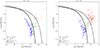 |
Fig. 1. BPT diagnostic diagram for CO-VG galaxies (left) and CO-CS galaxies (right). Blue points represent star-forming galaxies, green points represent composite galaxies, and red points represent AGN galaxies. The dashed line represents the demarcation proposed by Kewley et al. (2001), while the solid line corresponds to the curve introduced by Kauffmann et al. (2003a). |
3.1.5. Stellar masses
The stellar masses for both the comparison sample (Saintonge et al. 2017) and the CO-VG sample are obtained from the MPA/JHU catalogue, a comprehensive dataset provided by the Max Planck Institute for Astrophysics (MPA) in collaboration with Johns Hopkins University (JHU)4 (Kauffmann et al. 2003b; Brinchmann et al. 2004; Tremonti et al. 2004; Salim et al. 2007). The determination of total stellar mass is done through fits to the SDSS five-band (ugriz) photometry based on Kauffmann et al. (2003b) (see Table 4).
Properties for the CO-VG sample.
3.1.6. Star formation rate
For the CO-VG sample, we used the method of Duarte Puertas et al. (2017) to calculate the SFR based on Hα and Hβ fluxes from the SDSS data because the SDSS fibre has a limited size of 2.5″. The Hα fluxes were corrected using an empirical aperture correction derived from integral-field spectroscopic (IFS) observations of nearby galaxies (Iglesias-Páramo et al. 2016, 2013) and extinction was corrected using the Hα/Hβ ratio. The method is similar to that of MPIA/JHU (Brinchmann et al. 2004), but it incorporates an improved aperture correction, resulting in better agreement with other methods for low-mass galaxies (see Appendix A).
This method differs from the determination of the SFR for the comparison sample, which is based on the near-ultraviolet (NUV) flux from the Galaxy Evolution Explorer (GALEX, Martin et al. 2005; Morrissey et al. 2007) and the mid-infrared (MIR) emission from the Wide-field Infrared Survey Explorer (WISE, Wright et al. 2010), in a SFR ‘ladder’ approach as described in Janowiecki et al. (2017). For consistency with previous studies involving xCOLD GASS, we use this value of the SFR for the comparison sample.
We cannot apply the same method to the CO-VG sample because of the lack of GALEX or WISE data for a considerable number of objects (49 galaxies). We therefore chose to use the Hα fluxes as a SFR tracer for CO-VG, following Duarte Puertas et al. (2017). However, for this method, there were also a few galaxies (27 galaxies; 8 galaxies from the IRAM 30 m CO-CAVITY survey and 19 from the xCOLD GASS void galaxies subset) without the necessary high-quality Hα/Hβ lines. For those cases, we used GALEX and WISE data (for 24 galaxies) to determine the SFR following the procedure described in Janowiecki et al. (2017), and for the remaining 3 objects without NUV and/or W4 data we calculated the SFR from the W3 data following the prescription described in Leroy et al. (2019).
A comparison between these methods for galaxies with available data is given in Appendix A, where we show there is satisfactory agreement. The mean difference between the values of SFRNUV + MIR and SFRHα is 0.01 dex, and there is a difference of 0.1 dex between the values of SFRMIR and SFRHα.
4. Results
In this section, we examine the different properties of void galaxies in comparison with the CO-CS sample, such as the specific star-formation rate (sSFR = SFR/M⋆), the molecular gas mass fraction (MH2/M⋆), and the star formation efficiency (SFE = SFR/MH2) as functions of the stellar mass of the galaxy M⋆. To further refine this comparison, we divided the sample into four different categories based on their position relative to the SFMS (see Sect. 4.2 for details on the definition of the SFMS): Starbust (SB) galaxies that lie 0.3 dex or more above the SFMS, star-forming (SF) galaxies within the SFMS (±0.3 dex), TZ galaxies down to SFMS −0.155 dex, and red-sequence (RS) galaxies lying below this limit (see Janowiecki et al. 2020).
Additionally, we subdivided the sample into five different mass bins: log M⋆ [M⊙] = 9.0–9.5, 9.5–10.0, 10.0–10.5, 10.5–11.0, and 11.0–11.5. In order to obtain a robust statistical significance, we employ the Kaplan-Meier estimator (Kaplan & Meier 1958), which takes into account the upper limits when determining the mean value. As an additional test, the Kolmogorov–Smirnov (KS) test was also applied to each stellar bin to judge the significance of any differences found between the samples. Here, upper limits were treated as detections5.
Despite variations in the distributions of the samples (see Fig. 2), the differences are minimal when considering only galaxies within the SFMS, except for bins with mass log M⋆/M⊙ > 10.5, where the CO-CS sample exhibits a larger population of galaxies in comparison to the CO-VG sample. Therefore, for a straightforward comparison, the mean values are calculated and compared only for galaxies on the SFMS.
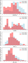 |
Fig. 2. Normalised histograms for the CO-VG (red) and the CO-CS (blue) to compare, from top to the bottom, the redshift, the stellar masses, and the sizes (R90, r, in arcsec and in kpc) of the galaxies in the two samples. |
4.1. Comparison of basic properties of galaxies in CO-VG and CO-CS
Figure 2 presents a comparison between the CO-VG sample and the CO-CS sample, examining their redshift, stellar masses, and sizes (defined by R90, r; which is the radius enclosing 90 percent of the Petrosian flux in the r band from SDSS; see Table 1). There is reasonable agreement between the redshift distributions of the two samples, with the CO-VG sample exhibiting a slight excess of nearby (z ≲ 0.023) objects and the CO-CS sample containing more distant (z ≳ 0.043) galaxies. The distributions in apparent size are also very similar, with a slight excess of small (R90, r ≲ 7″) galaxies in the CO-CS sample and more medium-sized (R90, r ∼ 10″) galaxies in CO-VG. In terms of physical size, as indicated in kiloparsecs (kpc), there is a slight excess of larger galaxies in the CO-CS sample compared to the CO-VG sample. The largest difference is in the distribution of stellar mass. The CO-VG sample contains more than twice as many low-mass galaxies (log M⋆/M⊙ < 10) as the CO-CS sample, while the CO-CS sample contains a larger fraction of high-mass (log M⋆/M⊙ > 10.5) galaxies. This difference has previously been identified in studies of void samples, and is also seen in hydrodynamical simulations (e.g. Illustris TNG, EAGLE), where it appears to mainly be due to the fact that the star formation histories (SFHs) of void galaxies tend to be slower than those exhibited by galaxies in denser environments (Alpaslan et al. 2015; Chen et al. 2017; Laigle et al. 2018; Rosas-Guevara et al. 2022; Domínguez-Gómez et al. 2023a; Rodríguez-Medrano et al. 2024). It is therefore necessary to take into account the stellar mass as a crucial parameter when analysing the two samples. Furthermore, it is not possible to draw any statistically significant conclusions for the highest mass bins (log M⋆ ≳ 11) due to the low number of galaxies in the CO-VG sample.
4.2. SFMS
We employed the SFMS established in Janowiecki et al. (2020, their Eq. 1) as a reference. Following these authors, we adopt ±0.3 dex to define the width of the SFMS, and also employ their division line (−1.55 dex below the SFMS) to separate the TZ and the RS.
Figure 3 shows a decreasing correlation between the sSFR and M⋆ for both the CO-VG sample and the comparison sample. The mean values of the CO-CS sample are slightly higher than expected from the SFMS, which is probably due to the fact that we excluded void, cluster, and AGN galaxies and therefore changed the CO-CS sample with respect to the sample used to derive the SFMS in Janowiecki et al. (2020). In any case, the differences are very small (see Table 6).
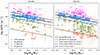 |
Fig. 3. Specific star formation rate as a function of stellar mass for the CO-VG sample (left) and the CO-CS sample (right). The SFMS is represented as a solid black line, and was derived as in Janowiecki et al. (2020, their Eq. 1). The dashed black lines represent the ±0.3 dex offset to the SFMS (Janowiecki et al. 2020) and the brown solid line represents the threshold of the RS, as also defined by Janowiecki et al. (2020, SFMS < 1.55 dex). Galaxies are colour coded according to their positions on the SFMS: (i) pink stars represent SB galaxies that lie above the SFMS, (ii) blue dots are SF galaxies within the SFMS (±0.3 dex), (iii) green diamonds are galaxies that lie in the TZ, and (iv) orange squares show RS galaxies below the TZ (SFMS < 1.55 dex). The mean sSFR per M⋆ bin is shown with a blue dashed line for the CO-VG and blue solid line for the CO-CS considering only those galaxy that belong to the SFMS. The extent of this line represents the width of the stellar mass bin. The error on the mean value is represented with a grey shadow. |
For SF galaxies, the mean values of sSFR are, for most mass bins, slightly lower for the CO-VG sample than for the CO-CS sample; although the difference is not significant (see Table 5). For SF galaxies, the distributions of CO-VG and CO-CS galaxies are similar. Above the SFMS, in the SB regime, the CO-VG sample is well distributed over the range of log M⋆/M⊙ = 9.0–10.5, while for the CO-CS sample the SB galaxies are more concentrated towards the mass bin log M⋆/M⊙ = 10.0–10.5. Below the SFMS, the CO-VG galaxies are on average much closer to the SFMS than the members of the comparison sample, and the CO-CS sample is also more populated at higher stellar masses. Almost all CO-VG galaxies below the SFMS are in the TZ region, and only a few galaxies are below this limit, in the RS region, which is mostly due to the selection of the objects (see Sect. 2.1).
Star formation rate for CO-VG and CO-CS galaxies: Mean values for galaxies on the SFMS.
We note that the statistical reliability of the results of the two highest mass bins for this and all subsequent relations discussed in this work is very limited due to the low number of galaxies in each of these bins, in particular for SF galaxies. In the mass bin of log M⋆/M⊙ = 10.5–11.0, there are only five galaxies in the CO-VG sample and in the adjacent mass bin (log M⋆/M⊙ = 11.0–11.5) there is only one galaxy in each sample, and so the results in this bin are only illustrative.
As the distance to the SFMS is a parameter that characterises the evolutionary path of galaxies we calculated, following Janowiecki et al. (2020, their Eq. 3), the distance to the SFMS, ΔSFMS, as
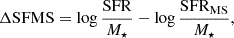
where SFRMS is the SFR corresponding to the SFMS value for a given M⋆. In Table 6, we present the mean and standard deviation of ΔSFMS for the SB, SFMS, and TZ galaxies of both samples, that is, the CO-VG sample and the CO-CS sample.
< ΔSFMS> measurements for CO-VG and CO-CS galaxies.
4.3. Molecular gas mass
Figure 4 shows the relation between the molecular gas mass fraction, MH2/M⋆, and M⋆ for both the CO-VG sample and the comparison sample. Similarly to the SFMS, we adopted the H2 main sequence relation, H2MS, from Janowiecki et al. (2020, their Eq. 5) and identify galaxies falling within ±0.2 dex of this relation as belonging to the H2MS. This relation was derived as a linear fit to the molecular gas mass fraction of the galaxies on the SFMS. Janowiecki et al. (2020) classified galaxies according to their gas content as gas normal (within the H2MS), gas rich (above this relation), or gas poor (below this relation). Following Eq. 7 of this latter publication, we define the distance to the H2MS as
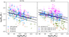 |
Fig. 4. Molecular gas mass fraction as a function of stellar mass for the CO-VG sample (left) and the CO-CS sample (right). The H2MS from Janowiecki et al. (2020) is represented as a solid black line. The dashed black lines represent the ±0.2 dex offset to the H2MS. Galaxies are colour coded according to their positions on the SFMS as described in Fig. 3. The mean logarithm of the molecular gas mass fraction per M⋆ bin is shown with a blue dashed line for the CO-VG and a blue solid line for the CO-CS considering only those galaxies that belong to the SFMS. The extent of this line represent the width of the stellar mass bin. The error of the mean value is represented with a grey shadow. The MH2 upper limits are represented with downward-pointing arrows. |
where MH2, MS is the MH2 corresponding to the H2MS value for a given M⋆.
There are no significant differences in terms of the mean values of the molecular gas mass fraction in different mass bins between SFMS galaxies in the CO-VG sample and those in the CO-CS sample (see Table 7). We note that the lowest mass bin has a high number of upper limits, making the results less reliable.
Molecular gas mass fraction for CO-VG and CO-CS galaxies: Mean values for galaxies on the SFMS.
In Fig. 5, we present a histogram of the distributions of ΔH2MS for three categories (SB, SFMS, and TZ) in both the CO-VG sample and the comparison sample. The mean and the median values, as well as the standard deviation for the ΔH2MS distributions, are summarised in Table 8. The three distributions exhibit overlap, especially in the case of the CO-VG sample. The distribution of the SFMS galaxies is similar for CO-CS and CO-VG galaxies, with no significant difference either in the mean or in the standard deviation of ΔH2MS. However, for the SB galaxies, there is a tentative difference, with the mean value of ΔH2MS for the CO-CS sample being shifted to higher values (by 0.07 dex, corresponding to 2σ) compared to the CO-VG sample. For the TZ galaxies, we find a similar trend, in the sense that the mean value for CO-VG galaxies is higher (i.e. closer to the SFMS value) than for the CO-CS sample by 0.27 dex (corresponding to 4σ). The trend for this galaxy group has, however, to be taken with caution because of the sparse sampling of the CO-VG sample, and in particular the lack of massive galaxies in the TZ, and the large number of upper limits.
 |
Fig. 5. Histograms of ΔH2MS for the CO-VG sample (left) and the comparison sample (right). The three categories of galaxies are colour coded with respect to their positions on the SFMS; (i) pink for SB galaxies above the SFMS, (ii) blue for SF galaxies within the SFMS (±0.3 dex), and (iii) green for galaxies that lie in the TZ. H2 detections are shown as full lines and non-detections as dotted histograms. |
< ΔH2MS> measurements for CO-VG and CO-CS galaxies.
In addition to their dependence on M⋆, the molecular gas properties also depend on the distance to the SFMS, ΔSFMS (see Saintonge et al. 2016; Tacconi et al. 2018; Janowiecki et al. 2020). Figure 6 shows the relation between ΔSFMS and ΔH2MS. There is a clear relation between the two quantities in the comparison sample. For the CO-VG sample, this relation has a higher dispersion and a smaller dynamic range in ΔH2MS. We used the linear least squares method to fit the data in both samples as ΔSFMS = a + m × ΔH2MS. We derived slopes of m = 0.95 ± 0.09 and 1.33 ± 0.06 and a = −0.03 ± 0.26 and −0.05 ± 0.03 for the CO-VG sample and the CO-CS sample, respectively. The correlation coefficients are r = 0.59 and 0.83 for the CO-VG sample and the CO-CS sample, respectively.
 |
Fig. 6. ΔSFMS as a function of ΔH2MS for the CO-VG sample (left) and the comparison sample (right). Galaxies are colour coded according to their position on the SFMS as described in Fig. 3. The blue and orange lines represent fits for the CO-VG sample and the comparison sample, respectively. The respective blue and orange shadows represent the 1σ dispersion of the fits. The CO non-detections are shown with leftward-pointing arrows. |
In conclusion, we find no major differences in the dependence of the molecular gas fraction on stellar mass for galaxies on the SFMS between galaxies in the CO-VG sample and those in the CO-CS sample. However, when considering the distribution of ΔH2MS and its relation to ΔSFMS, we find a positive correlation for both the CO-VG and the CO-CS sample, in the sense that the larger the distance in SFR from the SFMS, the larger the distance in the molecular gas mass fraction from the H2MS. However, this relation is tighter for galaxies in the CO-CS sample than for those in the CO-VG sample, for which the dynamical range in the molecular gas mass fraction also seems to be smaller.
4.4. Star formation efficiency
Figure 7 shows the relation between SFE and stellar mass (where SFE = SFR/MH2). For the SFMS galaxies in the comparison sample, a slightly decreasing trend is visible. This trend is not seen for the CO-VG sample, for which the relation seems to be constant across all mass bins. The different trends are also seen when comparing the mean values for the individual bins (Table 9). The low value of the KS test (p-value = 0.002) for the lowest mass bin confirms the difference in the trends at low stellar masses for the two samples. These trends remain the same when calculating the mean of all galaxies in each mass bin (i.e. taking together SB, SFMS, and TZ galaxies), and therefore they seem to be robust and to be the result of the different environments and independent of SF activity.
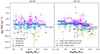 |
Fig. 7. Star formation efficiency as a function of stellar mass for the CO-VG sample (left) and the CO-CS (right) sample. Galaxies are colour coded according to their position on the SFMS as described in Fig. 3. The mean logarithm of the SFE per M⋆ bin is shown with a blue dashed line for the CO-VG and a blue solid line for the CO-CS sample, considering only those galaxies that belong to the SFMS. The extent of this line represent the width of the stellar mass bin. The error of the mean value is represented with a grey shadow. The lower limits are shown with upward-pointing arrows. |
Star formation efficiency for CO-VG and CO-CS galaxies: Mean values for galaxies on the SFMS.
CO(2–1)-to-CO(1–0) line ratio, R21, for CO-VG and CO-CS galaxies: Mean values.
Figure 8 shows the relation between the SFE and ΔSFMS for both the CO-VG and the CO-CS samples. A linear relationship is visible for both samples. We carried out a linear least square fit to the data in both samples, as log SFE = a + m × ΔSFMS. We derived slopes of m = 0.64 ± 0.03 and 0.55 ± 0.02 for the CO-VG sample and the CO-CS sample, respectively, and a = −9.0 ± 0.1 for both samples. For comparison, Fig. 8 also incorporates the relationship reported by Tacconi et al. (2018) for a large sample of galaxies at different redshifts (log SFE ∝ ΔSFMS0.44; here we arbitrarily adjust the abscissa to best fit our data). The slope derived for the CO-VG sample is steeper than that for the comparison sample, and is also steeper than the slope of Tacconi et al. (2018), suggesting a tendency of local void galaxies above the SFMS to show a relatively high SFE.
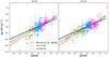 |
Fig. 8. Star formation efficiency as a function of SFMS distance for the CO-VG sample (left) and the comparison sample (right). Galaxies are colour coded according to their position on the SFMS as described in Fig. 3. The blue and orange lines represent fits for the CO-VG sample and the comparison sample, respectively, considering the four categories of galaxies. The respective blue and orange shadows represent the 1σ dispersion of the fits. The black thick line represents the power law found by Tacconi et al. (2018). |
4.5. Line intensity ratio (R21 = ICO(2 − 1)/ICO(1 − 0))
Figure 9 shows the correlation between the observed velocity-integrated intensities ICO(1 − 0) and ICO(2 − 1) for both samples. The observations of the CO(1–0) and CO(2–1) emission were carried out with different beam sizes. Therefore, in order to interpret the ratio between them, R21 = ICO(2 − 1)/ICO(1 − 0), one has to consider, in addition to the excitation temperature of the gas, two main parameters: the source size relative to the beam and the opacity of the molecular gas (see e.g. Solomon et al. 1997, Sect. 3.1.1, or Domínguez-Gómez et al. 2022, Appendix A). Following Domínguez-Gómez et al. (2022), we can derive from their Eq. A7 the expected values of R21 for optically thick gas in thermal equilibrium in the case of a point-like or a very extended source: For emission with a point-like distribution, we expect a ratio of R21 =  (with
(with  being the central intrinsic brightness ratio and ΘB the FWHM of the respective beams). On the other hand, for a source that is more extended than the beams, or for beam-matched observations with ΘB(CO1 − 0) = ΘB(CO2 − 1), we expect R21
 .
.
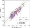 |
Fig. 9. ICO(2 − 1) and ICO(1 − 0) line emission (on the Tmb temperature scale) for the CO-VG sample and the CO-CS sample. To guide the eye, we include lines for fixed ratios between ICO(2 − 1) and ICO(1 − 0). |
In order to interpret R21 from our observations with different beam sizes, we need to take the ratio between source and beam size into account. In Fig. 10 we therefore show the relation between R21 and R90, r, which parameterises the source size. We consider two cases separately in order to be able to calculate the mean values with the Kaplan-Meier estimator, which does not allow upper and lower limits to be mixed: (i) subsamples including galaxies with detection and upper limits in R21, that is, data points derived from detections ICO(1 − 0) and detections or upper limits in ICO(2 − 1), and ii) subsamples including galaxies with detection and lower limits in R21, that is, data points derived from detections ICO(2 − 1) and detections or upper limits in ICO(1 − 0). In the figures, we include lines showing the theoretically expected R21 ratios for different intrinsic central brightness temperature ratios, following Domínguez-Gómez et al. (2022). These theoretical ratios are valid under the assumption that the distribution of the CO emission decreases exponentially with a scale length of 0.2 × r25 (see Sect. 3.1.2). In addition, the mean values for different R90, r bins for both samples are plotted.
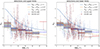 |
Fig. 10. Observed line-intensity ratio R21 = ICO(2 − 1)/ICO(1 − 0) as a function of the r-Petrosian R90, r. Left panel: Only detections and upper limits (i.e. data points with non-detections in ICO(1 − 0) were not considered). Right panel: Only detections and lower limits (i.e. data points with non-detections in ICO(2 − 1) were not considered. |
We find for both samples that R21 decreases with R90, r, as theoretically expected. The values of R21 for both samples are compatible within the errors for most of the bins that contain a significant number of galaxies (n≳ 10). Only in the radial bin 15″ < R90, r < 20″ is there a higher R21 (by ∼3σ) for CO-CS galaxies. In both samples, the mean values of R21 follow the predicted relation reasonably well for an intrinsic central brightness temperature ratio of  . This value is consistent with optically thick gas with a temperature of 5–10 K (
 = 0.6 corresponds to gas with a temperature of ∼5 K, 0.8 to ∼10 K, and 0.9 to ∼21 K, and higher excitation temperatures yield a line ratio of ∼1; Braine & Combes 1992; Leroy et al. 2009).
The value of  agrees well with results for beam-matched line ratios, R21, from other galaxy samples, which indicates that the ratio in discs is typically R21 ∼0.5–0.8, with higher values (∼1) in the centres (Casoli et al. 1991; Leroy et al. 2009). In agreement with this, Braine & Combes (1993) found an average line ratio of 0.89 ± 0.6 for the central regions of a small sample of nearby spiral galaxies. Furthermore, Braine & Combes (1992) found a small difference in their sample for isolated galaxies (R21 = 0.82) and perturbed objects (R21 = 1.11). Casasola et al. (2015) found R21 ∼0.6–0.9 for four low-luminosity AGN from the NUclei of GAlaxies (NUGA) survey. Also, for the Milky Way, typical line ratios of ∼0.6–0.8 in the disc and ∼1 towards the Galactic centre were found (Sakamoto et al. 1995; Oka et al. 1996, 1998).
5. Discussion
Simulations and observations suggest that galaxy properties are strongly influenced by their large-scale environment. However, there remains no clear consensus regarding the concrete effect that this relation has on the gas and the SF. While simulations generally predict a suppression of SF in present-day galaxies with decreasing distance from filaments (e.g. Hasan et al. 2023; Bulichi et al. 2024), observations suggest the opposite is true. Some studies find an enhancement of the sSFR in filament galaxies (Vulcani et al. 2019; Darvish et al. 2014), which is possibly caused by filaments assisting gas cooling and thereby enhancing star formation. However, within filaments, other phenomena with opposing consequences may also occur, such as gas-stripping, which can quench star formation (e.g. Chen et al. 2017; Kraljic et al. 2018; Winkel et al. 2021). In any case, these large-scale environmental processes are expected to mostly affect the atomic hydrogen (HI) supply of the galaxies (see e.g. Hasan et al. 2023), and not directly the molecular gas, which is formed from the HI in galaxies. Observations of HI will be important in order to search for differences between galaxies in voids and those in denser environments, and are in progress for the CAVITY project.
In the present study, we focus on observations of the molecular gas mass to find out whether the amount of molecular gas or the SFE depend on the large-scale environment, and, in particular, if there are differences between galaxies in voids and those in filaments and walls. Our large sample (200 void galaxies in CO-VG and a similar number of galaxies in filaments and walls in CO-CS) allows a solid statistical comparison between the two environments. In order to provide a reliable comparison, we made sure that the relevant parameters of this study (SFR, molecular gas mass, and stellar mass) were derived consistently in both samples and in addition we excluded galaxies with AGN from our study in order to prevent any ambiguities. The two most important internal parameters that control the molecular gas mass fraction and the SFE are stellar mass and distance to the SFMS. Accordingly, we based our comparison on these two parameters.
With respect to the molecular gas mass fraction, MH2/M⋆, we do not find significant differences between CO-VG and CO-CS across all mass bins for the SFMS galaxies. This finding is consistent with the results of Domínguez-Gómez et al. (2022), who analysed similar properties in a pilot sample of about 20 void galaxies. When also considering SB and TZ galaxies, we find a tentative indication that the dynamic range of MH2/M⋆ is higher in the comparison sample than in the CO-VG sample, suggesting that the environment could affect the molecular gas content in galaxies.
On the other hand, a much clearer difference is observed in the variation of the SFE with respect to stellar mass between galaxies in CO-VG and in CO-CS (see Fig. 7). For the comparison sample, the mean SFE exhibits a decline of approximately 5% from the highest to the lowest value when considering only the first four most populated mass bins (log M⋆/M⊙, = 9.0–11.0). This trend aligns with prior investigations (see e.g. Saintonge et al. 2017; Lisenfeld et al. 2023, for the highest mass galaxies). Quite differently, the SFE–stellar mass relationship in the CO-VG sample remains almost constant in this mass range. The clearest difference is in the lowest mass bin (log M⋆/M⊙, = 9.0–9.5), where the SFE in CO-VG lies 0.24 dex (corresponding to > 3σ, and KS p-value ∼0.002) below the value of the comparison sample. This means that at low stellar masses, SF is less efficient in void galaxies than in galaxies residing in filaments and walls.
The cause of this difference is not entirely clear. A variation of the SFE might be associated with a change in the properties of the molecular gas. We note that CO(1–0) probes relatively low-density gas (∼3000 cm−3), part of which might not be associated with giant molecular clouds (GMCs) able to form stars. Other molecules, such as HCN(1–0), with higher critical densities are better tracers of the star-forming molecular gas (e.g. Gao & Solomon 2004; Graciá-Carpio et al. 2006; García-Burillo et al. 2012). Thus, the variation of the fraction of high-density molecular gas to low-density molecular gas – which is unable to form stars – across the SFMS might be the reason for the observed variation of the SFE in CO-CS (see Saintonge et al. 2017); if this is the case, such a variation might be absent in the void galaxies. The reason for such a variation – or lack of it – is, however, not obvious from the single-dish data. Resolved data are needed to shed more light on this subject. Resolved studies relying on CO and HCN (Usero et al. 2015; Bigiel et al. 2016; Jiménez-Donaire et al. 2019) have shown that indeed the dense molecular gas fraction depends on many galactic properties, such as the stellar or gas surface density, the molecular-to-atomic mass ratio, and the dynamical equilibrium pressure. Surprisingly, the ratio between SFR and dense (i.e. HCN traced) molecular gas varies considerably – more than the CO-traced SFE – with galactic environmental conditions. Studies at the scale of individual GMCs in different galaxies have shown that their properties are driven by their galactic environment on kpc scales (Sun et al. 2022), and that the pressure of the hydrostatic ISM plays a role in shaping their density and velocity dispersion (Hughes et al. 2013). Thus, it might be possible that these effects play a role in the (small) differences that we have found between CO-VG and CO-CS galaxies, most likely due to effects that the large-scale intergalactic environment might have on the galactic ISM. High-resolution observations with ALMA are currently under way for the CAVITY sample in order to make progress in this regard.
Another internal mechanism has been proposed to be responsible for quenching, known as ‘morphological quenching’ (Martig et al. 2009; Bluck et al. 2014). According to these works, the presence of a bulge can stabilise the gas and inhibit star formation. Simulations have confirmed that this relation has a causal basis through dynamical effects (‘dynamical quenching’; Gensior et al. 2020) linked to the central spheroids, which increase the gas velocity dispersion and stabilise the region against SF. This mechanism may help to explain the observed decrease in the SFE with stellar mass, given that the bulge fraction also increases with stellar mass. If this mechanism were to explain the difference found between the void galaxies and the comparison sample in terms of SFE – and in particular the higher SFE at low masses for void galaxies–, a smaller bulge-to-disc ratio for low-mass galaxies in voids would be a necessary condition; this could be explored by further analysis of the optical CAVITY data.
6. Conclusions
In this paper, following the CO-CAVITY pilot project containing CO data for 20 void galaxies (Domínguez-Gómez et al. 2022), we present data for the molecular gas mass of a large sample of void galaxies (200 galaxies, referred to here as the CO-VG sample), which we analysed and compared to a similar-sized comparison sample (265 galaxies, the CO-CS sample). This analysis is based on the largest statistical data set for the molecular gas in void galaxies so far. Our aim is to study the molecular gas content and properties in void galaxies and to search for possible differences between them and galaxies that inhabit denser structures.
We present new data of the CO(1–0) and CO(2–1) line emission observed with the IRAM 30 m IRAM telescope for a sample of 106 galaxies belonging to the CAVITY project (Pérez et al. 2024). For CO(1–0), we recorded 64 detections, 9 tentative detections, and 33 non-detections, while for CO(2–1), we obtained 63 detections, 8 tentative detections, and 35 non-detections. In addition to the 106 CAVITY galaxies, we included a sample of 16 CO-VGS galaxies that were previously observed using the IRAM 30 m telescope (Domínguez-Gómez et al. 2022), and 89 xCOLD GASS void galaxies. Finally, we exclude 11 galaxies classified as AGN, and thus the final CO-VG sample is composed of 200 galaxies.
We selected the xCOLD GASS survey as our comparison sample after removing void and cluster galaxies, as well as galaxies with AGN. We conducted an analysis of the sSFR, the molecular gas mass fraction, and the SFE as a function of stellar mass and distance to the SFMS. Below, we summarise our key conclusions.
-
The distribution of the molecular gas mass fraction as a function of M⋆ of galaxies on the SFMS is overall consistent with the distribution of the comparison sample. For starburst galaxies, defined as objects located above the SFMS, the mean log(MH2/M⋆) is slightly lower in CO-VG than in CO-CS galaxies, while it is higher in galaxies in the TZ, which are defined as objects below the SFMS, indicating that the distribution of log(MH2/M⋆) as a function of distance from the SFMS might be more concentrated than for the comparison sample.
-
The mean values for the SFE for void galaxies on the SFMS show no trend with M⋆ in contrast to the comparison sample; for void galaxies, the mean value of SFE ranges between ∼−8.94 and −8.99, whereas in the comparison sample the SFE decreases from −8.73 to −9.12 from the lowest to the highest mass bin. These different trends might be related to differences in the properties of the molecular gas at the spatial scales of GMCs, which are possibly caused by the different environments. However, the exact cause is unclear and higher-resolution observations are necessary to make progress in this regard.
-
The CO(2–1)/CO(1–0) intensity ratio, R21, shows a decreasing trend with galactic radius, R90, r, for both samples, and is compatible, within the scatter, with the intrinsic brightness temperature (i.e. beam-matched) ratio of R21 ∼ 0.7. This ratio is consistent with optically thick, thermalised emission with an excitation temperature of 5–10 K, in agreement with other studies based on beam-matched observations.
This is one of the first studies of molecular gas in a large number of void galaxies. Our analysis shows that there are no differences between void galaxies and galaxies within filaments and walls in terms of the total amount of molecular gas, but there are differences in the SFE, suggesting that the physical mechanisms affecting the SFE are different in void galaxies. Further data provided by the CAVITY project (IFU, and high-resolution CO and HI) will enable further elucidation of the distinctions between void galaxies and those within filaments and walls.
Data availability
Full Tables 1–4 are available at the CDS via anonymous ftp to cdsarc.cds.unistra.fr (130.79.128.5) or via https://cdsarc.cds.unistra.fr/viz-bin/qcat?J/A+A/692/A125.
The observed spectra of the CO(1–0) and CO(2–1) emission lines of the CO-CAVITY galaxies are available on Zenodo https://zenodo.org/records/13981624.
The KS test is a statistical tool used to compare the characteristics of two distinct sample distributions. The KS test evaluates whether two samples come from the same mother sample. A p-value of below 0.05 indicates with reliability higher than 95% that both samples come from different mother samples, whereas for higher p-values, no firm conclusions can be drawn.
Acknowledgments
We thank the referee for very constructive comments improving the content and presentation of this paper. Thanks to the staff at IRAM Pico Veleta for their support during the observations. This work is based on observations carried out with the IRAM 30 m telescope. IRAM is supported by INSU/CNRS (France), MPG (Germany) and IGN (Spain). We acknowledge financial support by the research projects AYA2017-84897-P, PID2020-113689GB-I00, and PID2020-114414GB-I00, financed by MCIN/AEI/10.13039/501100011033, the project A-FQM-510-UGR20 financed from FEDER/Junta de Andalucía-Consejería de Transformación Económica, Industria, Conocimiento y Universidades/Proyecto and by the grants P20-00334 and FQM108, financed by the Junta de Andalucía (Spain). MIR acknowledge financial support from Grant AST22.4.4, funded by Consejería de Universidad, Investigación e Innovación and Gobierno de España and Unión Europea – NextGenerationEU. Funding for this work/research was provided by the European Union (MSCA EDUCADO, GA 101119830). BB acknowledges financial support from the Grant AST22-4.4 funded by Consejería de Universidad, Investigación e Innovación and Gobierno de España and Unión Europea – NextGenerationEU, and by the research project PID2020-113689GB-I00 financed by MCIN/AEI/10.13039/501100011033. DE acknowledges support from a Beatriz Galindo senior fellowship (BG20/00224) from the Spanish Ministry of Science and Innovation. J. F-B acknowledges support from the PID 2022-140869 NB-100 grant from the Spanish Ministry of Science and Innovation. GTR acknowledges financial support from the research project PRE2021-098736, funded by MCIN/AEI/10.13039/501100011033 and FSE+. IP acknowledges financial support from the grant AST22.4.4, funded by Consejería de Universidad, Investigaciń e Innovación and Gobierno de España and Unión Europea – NextGenerationEU, and by PID2020-113689GB-I00, financed by MCIN/AEI. KK gratefully acknowledges funding from the Deutsche Forschungsgemeinschaft (DFG, German Research Foundation) in the form of an Emmy Noether Research Group (grant number KR4598/2-1, PI Kreckel) and the European Research Council’s starting grant ERC StG-101077573 (“ISM-METALS”). LSM acknowledges support from Juan de la Cierva fellowship (IJC2019-041527-I). M.A-F. acknowledges support from the Emergia program (EMERGIA20-38888) from Consejería de Universidad, Investigación e Innovación de la Junta de Andalucía. M.S.P. and A.B. acknowledge the support of the Spanish Ministry of Science, Innovation and Universities through the project PID-2021-122544NB-C43. PVG acknowledges that the project that gave rise to these results received the support of a fellowship from “la Caixa” Foundation (ID 100010434). The fellowship code is B005800. SBD acknowledges financial support by the grant AST22.4.4, funded by Consejería de Universidad, Investigación e Innovación and Gobierno de España and Unión Europea – NextGeneration EU, also funded by PID2020-113689GB-I00, financed by MCIN/AEI. RGB acknowledges financial support from the Severo Ochoa grant CEX2021-001131-S funded by MCIN/AEI/ 10.13039/501100011033 and grant PID2022-141755NB-I00. SDP acknowledges financial support from Juan de la Cierva Formación fellowship (FJC2021-047523-I) financed by MCIN/AEI/10.13039/501100011033 and by the European Union ‘NextGenerationEU’/PRTR, Ministerio de Economía y Competitividad under grants PID2019-107408GB-C44, PID2022-136598NB-C32, and is grateful to the Natural Sciences and Engineering Research Council of Canada, the Fonds de Recherche du Québec, and the Canada Foundation for Innovation for funding. TRL acknowledges support from Juan de la Cierva fellowship (IJC2020-043742-I). This work made use of the following software packages: astropy (Astropy Collaboration 2013, 2018, 2022), Jupyter (Perez & Granger 2007; Kluyver et al. 2016), matplotlib (Hunter 2007), numpy (Harris et al. 2020), pandas (Wes McKinney 2010; The pandas development team 2024), python (Van Rossum & Drake 2009), scipy (Virtanen et al. 2020; Gommers et al. 2024), astroquery (Ginsburg et al. 2019, 2024) and scikit-learn (Pedregosa et al. 2011; Buitinck et al. 2013; Grisel et al. 2024). Software citation information aggregated using https://www.tomwagg.com/software-citation-station/ (Wagg & Broekgaarden 2024a,b). This research has made use of the NASA/IPAC Extragalactic Database, which is funded by the National Aeronautics and Space Administration and operated by the California Institute of Technology. Funding for SDSS-III has been provided by the Alfred P. Sloan Foundation, the Participating Institutions, the National Science Foundation, and the U.S. Department of Energy Office of Science. The SDSS-III Web site is http://www.sdss3.org/. The SDSS-IV site is http://www.sdss.org.
References
- Abazajian, K. N., Adelman-McCarthy, J. K., Agüeros, M. A., et al. 2009, ApJS, 182, 543 [Google Scholar]
- Accurso, G., Saintonge, A., Catinella, B., et al. 2017, MNRAS, 470, 4750 [NASA ADS] [Google Scholar]
- Alpaslan, M., Driver, S., Robotham, A. S. G., et al. 2015, MNRAS, 451, 3249 [Google Scholar]
- Aragón-Calvo, M. A., Jones, B. J. T., van de Weygaert, R., & van der Hulst, J. M. 2007, A&A, 474, 315 [NASA ADS] [CrossRef] [EDP Sciences] [Google Scholar]
- Asplund, M., Grevesse, N., Sauval, A. J., Allende Prieto, C., & Kiselman, D. 2004, A&A, 417, 751 [NASA ADS] [CrossRef] [EDP Sciences] [Google Scholar]
- Astropy Collaboration (Robitaille, T. P., et al.) 2013, A&A, 558, A33 [NASA ADS] [CrossRef] [EDP Sciences] [Google Scholar]
- Astropy Collaboration (Price-Whelan, A. M., et al.) 2018, AJ, 156, 123 [Google Scholar]
- Astropy Collaboration (Price-Whelan, A. M., et al.) 2022, ApJ, 935, 167 [NASA ADS] [CrossRef] [Google Scholar]
- Baker, W. M., Maiolino, R., Bluck, A. F. L., et al. 2022, MNRAS, 510, 3622 [NASA ADS] [CrossRef] [Google Scholar]
- Baldwin, J. A., Phillips, M. M., & Terlevich, R. 1981, PASP, 93, 5 [Google Scholar]
- Beygu, B., Kreckel, K., van de Weygaert, R., van der Hulst, J. M., & van Gorkom, J. H. 2013, AJ, 145, 120 [NASA ADS] [CrossRef] [Google Scholar]
- Beygu, B., Peletier, R. F., van der Hulst, J. M., et al. 2017, MNRAS, 464, 666 [NASA ADS] [CrossRef] [Google Scholar]
- Bigiel, F., Leroy, A. K., Jiménez-Donaire, M. J., et al. 2016, ApJ, 822, L26 [NASA ADS] [CrossRef] [Google Scholar]
- Bluck, A. F. L., Mendel, J. T., Ellison, S. L., et al. 2014, MNRAS, 441, 599 [NASA ADS] [CrossRef] [Google Scholar]
- Bolatto, A. D., Wolfire, M., & Leroy, A. K. 2013, ARA&A, 51, 207 [CrossRef] [Google Scholar]
- Bond, J. R., Kofman, L., & Pogosyan, D. 1996, Nature, 380, 603 [NASA ADS] [CrossRef] [Google Scholar]
- Braine, J., & Combes, F. 1992, A&A, 264, 433 [NASA ADS] [Google Scholar]
- Braine, J., & Combes, F. 1993, A&A, 269, 7 [NASA ADS] [Google Scholar]
- Brinchmann, J., Charlot, S., White, S. D. M., et al. 2004, MNRAS, 351, 1151 [Google Scholar]
- Buitinck, L., Louppe, G., Blondel, M., et al. 2013, ECML PKDD Workshop: Languages for Data Mining and Machine Learning, 108 [Google Scholar]
- Bulichi, T.-E., Davé, R., & Kraljic, K. 2024, MNRAS, 529, 2595 [NASA ADS] [CrossRef] [Google Scholar]
- Bundy, K., Bershady, M. A., Law, D. R., et al. 2015, ApJ, 798, 7 [Google Scholar]
- Casasola, V., Hunt, L., Combes, F., & García-Burillo, S. 2015, A&A, 577, A135 [NASA ADS] [CrossRef] [EDP Sciences] [Google Scholar]
- Casoli, F., Dupraz, C., Combes, F., & Kazes, I. 1991, A&A, 251, 1 [NASA ADS] [Google Scholar]
- Cautun, M. C. 2014, Ph.D. Thesis, University of Groningen, Netherlands [Google Scholar]
- Chen, Y.-C., Ho, S., Mandelbaum, R., et al. 2017, MNRAS, 466, 1880 [NASA ADS] [CrossRef] [Google Scholar]
- Conrado, A. M., González Delgado, R. M., García-Benito, R., et al. 2024, A&A, 687, A98 [NASA ADS] [CrossRef] [EDP Sciences] [Google Scholar]
- Constantin, A., Hoyle, F., & Vogeley, M. S. 2008, ApJ, 673, 715 [NASA ADS] [CrossRef] [Google Scholar]
- Cormier, D., Madden, S. C., Lebouteiller, V., et al. 2014, A&A, 564, A121 [NASA ADS] [CrossRef] [EDP Sciences] [Google Scholar]
- Darvish, B., Sobral, D., Mobasher, B., et al. 2014, ApJ, 796, 51 [NASA ADS] [CrossRef] [Google Scholar]
- Das, M., Saito, T., Iono, D., Honey, M., & Ramya, S. 2016, The Zeldovich Universe: Genesis and Growth of the Cosmic Web, 610 [Google Scholar]
- Domínguez-Gómez, J., Lisenfeld, U., Pérez, I., et al. 2022, A&A, 658, 124 [Google Scholar]
- Domínguez-Gómez, J., Pérez, I., Ruiz-Lara, T., et al. 2023a, Nature, 619, 269 [CrossRef] [Google Scholar]
- Domínguez-Gómez, J., Pérez, I., Ruiz-Lara, T., et al. 2023b, A&A, 680, A111 [NASA ADS] [CrossRef] [EDP Sciences] [Google Scholar]
- Duarte Puertas, S., Vilchez, J. M., Iglesias-Páramo, J., et al. 2017, A&A, 599, A71 [NASA ADS] [CrossRef] [EDP Sciences] [Google Scholar]
- Duarte Puertas, S., Vilchez, J. M., Iglesias-Páramo, J., et al. 2022, A&A, 666, A186 [NASA ADS] [CrossRef] [EDP Sciences] [Google Scholar]
- Elbaz, D., Daddi, E., Le Borgne, D., et al. 2007, A&A, 468, 33 [NASA ADS] [CrossRef] [EDP Sciences] [Google Scholar]
- Florez, J., Berlind, A. A., Kannappan, S. J., et al. 2021, ApJ, 906, 97 [NASA ADS] [CrossRef] [Google Scholar]
- Gao, Y., & Solomon, P. M. 2004, ApJ, 606, 271 [NASA ADS] [CrossRef] [Google Scholar]
- García-Burillo, S., Usero, A., Alonso-Herrero, A., et al. 2012, A&A, 539, A8 [Google Scholar]
- Gensior, J., Kruijssen, J. M. D., & Keller, B. W. 2020, MNRAS, 495, 199 [NASA ADS] [CrossRef] [Google Scholar]
- Ginsburg, A., Sipőcz, B. M., Brasseur, C. E., et al. 2019, AJ, 157, 98 [Google Scholar]
- Ginsburg, A., Sipőcz, B., Brasseur, C. E., et al. 2024, https://doi.org/10.5281/zenodo.10799414 [Google Scholar]
- Gommers, R., Virtanen, P., Haberland, M., et al. 2024, https://doi.org/10.5281/zenodo.10909890 [Google Scholar]
- Graciá-Carpio, J., García-Burillo, S., Planesas, P., & Colina, L. 2006, ApJ, 640, L135 [CrossRef] [Google Scholar]
- Grisel, O., Mueller, A., Buitinck, L., et al. 2024, https://doi.org/10.5281/zenodo.10666857 [Google Scholar]
- Gunawardhana, M. L. P., Hopkins, A. M., Bland-Hawthorn, J., et al. 2013, MNRAS, 433, 2764 [NASA ADS] [CrossRef] [Google Scholar]
- Harris, C. R., Millman, K. J., van der Walt, S. J., et al. 2020, Nature, 585, 357 [NASA ADS] [CrossRef] [Google Scholar]
- Hasan, F., Burchett, J. N., Hellinger, D., et al. 2023, ArXiv e-prints [arXiv:2311.01443] [Google Scholar]
- Hughes, A., Meidt, S. E., Colombo, D., et al. 2013, ApJ, 779, 46 [NASA ADS] [CrossRef] [Google Scholar]
- Hunter, J. D. 2007, Comput. Sci. Eng., 9, 90 [NASA ADS] [CrossRef] [Google Scholar]
- Iglesias-Páramo, J., Vílchez, J. M., Galbany, L., et al. 2013, A&A, 553, L7 [NASA ADS] [CrossRef] [EDP Sciences] [Google Scholar]
- Iglesias-Páramo, J., Vílchez, J. M., Rosales-Ortega, F. F., et al. 2016, ApJ, 826, 71 [Google Scholar]
- Janowiecki, S., Catinella, B., Cortese, L., et al. 2017, MNRAS, 466, 4795 [NASA ADS] [Google Scholar]
- Janowiecki, S., Catinella, B., Cortese, L., Saintonge, A., & Wang, J. 2020, MNRAS, 493, 1982 [Google Scholar]
- Jiménez-Donaire, M. J., Bigiel, F., Leroy, A. K., et al. 2019, ApJ, 880, 127 [CrossRef] [Google Scholar]
- Kaplan, E. L., & Meier, P. 1958, J. Am. Stat. Assoc., 53, 457 [Google Scholar]
- Kauffmann, G., Heckman, T. M., Tremonti, C., et al. 2003a, MNRAS, 346, 1055 [Google Scholar]
- Kauffmann, G., Heckman, T. M., White, S. D. M., et al. 2003b, MNRAS, 341, 33 [Google Scholar]
- Kennicutt, R. C., Jr. 1998, ARA&A, 36, 189 [Google Scholar]
- Kewley, L. J., Dopita, M. A., Sutherland, R. S., Heisler, C. A., & Trevena, J. 2001, ApJ, 556, 121 [Google Scholar]
- Kluyver, T., Ragan-Kelley, B., Pérez, F., et al. 2016, ELPUB, 87 [Google Scholar]
- Kraljic, K., Arnouts, S., Pichon, C., et al. 2018, MNRAS, 474, 547 [Google Scholar]
- Kreckel, K. 2011, Am. Astron. Soc. Meet. Abstr., 217, 211.03 [NASA ADS] [Google Scholar]
- Kreckel, K., Platen, E., Aragón-Calvo, M. A., et al. 2012, AJ, 144, 16 [Google Scholar]
- Laigle, C., Pichon, C., Arnouts, S., et al. 2018, MNRAS, 474, 5437 [Google Scholar]
- Leroy, A. K., Walter, F., Bigiel, F., et al. 2009, AJ, 137, 4670 [Google Scholar]
- Leroy, A. K., Sandstrom, K. M., Lang, D., et al. 2019, ApJS, 244, 24 [Google Scholar]
- Libeskind, N. I., van de Weygaert, R., Cautun, M., et al. 2018, MNRAS, 473, 1195 [NASA ADS] [CrossRef] [Google Scholar]
- Lisenfeld, U., Espada, D., Verdes-Montenegro, L., et al. 2011, A&A, 534, A102 [NASA ADS] [CrossRef] [EDP Sciences] [Google Scholar]
- Lisenfeld, U., Xu, C. K., Gao, Y., et al. 2019, A&A, 627, A107 [NASA ADS] [CrossRef] [EDP Sciences] [Google Scholar]
- Lisenfeld, U., Ogle, P. M., Appleton, P. N., Jarrett, T. H., & Moncada-Cuadri, B. M. 2023, A&A, 673, A87 [NASA ADS] [CrossRef] [EDP Sciences] [Google Scholar]
- Madden, S. C., Rémy-Ruyer, A., Galametz, M., et al. 2013, PASP, 125, 600 [NASA ADS] [CrossRef] [Google Scholar]
- Martig, M., Bournaud, F., Teyssier, R., & Dekel, A. 2009, ApJ, 707, 250 [Google Scholar]
- Martin, D. C., Fanson, J., Schiminovich, D., et al. 2005, ApJ, 619, L1 [Google Scholar]
- Martin, D. C., Small, T., Schiminovich, D., et al. 2007, ApJS, 173, 415 [NASA ADS] [CrossRef] [Google Scholar]
- McKinney, W., 2010, in Proceedings of the 9th Python in Science Conference, 56 [CrossRef] [Google Scholar]
- Morrissey, P., Conrow, T., Barlow, T. A., et al. 2007, ApJS, 173, 682 [Google Scholar]
- Noeske, K. G., Weiner, B. J., Faber, S. M., et al. 2007, ApJ, 660, L43 [CrossRef] [Google Scholar]
- Oka, T., Hasegawa, T., Handa, T., Hayashi, M., & Sakamoto, S. 1996, ApJ, 460, 334 [NASA ADS] [CrossRef] [Google Scholar]
- Oka, T., Hasegawa, T., Sato, F., Tsuboi, M., & Miyazaki, A. 1998, ApJS, 118, 455 [Google Scholar]
- Pan, D. C., Vogeley, M. S., Hoyle, F., Choi, Y.-Y., & Park, C. 2012, MNRAS, 421, 926 [NASA ADS] [CrossRef] [Google Scholar]
- Park, C., Choi, Y.-Y., Vogeley, M. S., et al. 2007, ApJ, 658, 898 [Google Scholar]
- Pedregosa, F., Varoquaux, G., Gramfort, A., et al. 2011, J. Mach. Learn. Res., 12, 2825 [Google Scholar]
- Peebles, P. J. E. 2001, ApJ, 557, 495 [NASA ADS] [CrossRef] [Google Scholar]
- Perez, F., & Granger, B. E. 2007, Comput. Sci. Eng., 9, 21 [Google Scholar]
- Pérez, I., Verley, S., Sánchez-Menguiano, L., et al. 2024, A&A, 689, A213 [NASA ADS] [CrossRef] [EDP Sciences] [Google Scholar]
- Pettini, M., & Pagel, B. E. J. 2004, MNRAS, 348, L59 [NASA ADS] [CrossRef] [Google Scholar]
- Rodríguez-Medrano, A. M., Springel, V., Stasyszyn, F. A., & Paz, D. J. 2024, MNRAS, 528, 2822 [CrossRef] [Google Scholar]
- Rojas, R. R., Vogeley, M. S., Hoyle, F., & Brinkmann, J. 2004, ApJ, 617, 50 [NASA ADS] [CrossRef] [Google Scholar]
- Rojas, R. R., Vogeley, M. S., Hoyle, F., & Brinkmann, J. 2005, ApJ, 624, 571 [NASA ADS] [CrossRef] [Google Scholar]
- Rosas-Guevara, Y., Tissera, P., Lagos, C. d. P., Paillas, E., & Padilla, N. 2022, MNRAS, 517, 712 [NASA ADS] [CrossRef] [Google Scholar]
- Sage, L. J., Weistrop, D., Cruzen, S., & Kompe, C. 1997, AJ, 114, 1753 [NASA ADS] [CrossRef] [Google Scholar]
- Saintonge, A., Catinella, B., Cortese, L., et al. 2016, MNRAS, 462, 1749 [Google Scholar]
- Saintonge, A., Catinella, B., Tacconi, L. J., et al. 2017, ApJS, 233, 22 [Google Scholar]
- Sakamoto, S., Hasegawa, T., Hayashi, M., Handa, T., & Oka, T. 1995, ApJS, 100, 125 [NASA ADS] [CrossRef] [Google Scholar]
- Salim, S., Rich, R. M., Charlot, S., et al. 2007, ApJS, 173, 267 [NASA ADS] [CrossRef] [Google Scholar]
- Schmidt, M. 1959, ApJ, 129, 243 [NASA ADS] [CrossRef] [Google Scholar]
- Solomon, P. M., Downes, D., Radford, S. J. E., & Barrett, J. W. 1997, ApJ, 478, 144 [NASA ADS] [CrossRef] [Google Scholar]
- Sun, J., Leroy, A. K., Rosolowsky, E., et al. 2022, AJ, 164, 43 [NASA ADS] [CrossRef] [Google Scholar]
- Tacconi, L. J., Genzel, R., Saintonge, A., et al. 2018, ApJ, 853, 179 [Google Scholar]
- Tacconi, L. J., Genzel, R., & Sternberg, A. 2020, ARA&A, 58, 157 [NASA ADS] [CrossRef] [Google Scholar]
- Tempel, E., Tuvikene, T., Kipper, R., & Libeskind, N. I. 2017, A&A, 602, 100 [Google Scholar]
- The pandas development team 2024, https://doi.org/10.5281/zenodo.10697587 [Google Scholar]
- Tremonti, C. A., Heckman, T. M., Kauffmann, G., et al. 2004, ApJ, 613, 898 [Google Scholar]
- Usero, A., Leroy, A. K., Walter, F., et al. 2015, AJ, 150, 115 [Google Scholar]
- van de Weygaert, R. 2016, IAU Symp., 308, 493 [NASA ADS] [Google Scholar]
- van de Weygaert, R., & Bond, J. R. 2008, Lect. Notes Phys., 740, 335 [NASA ADS] [CrossRef] [Google Scholar]
- van de Weygaert, R., Kreckel, K., Platen, E., et al. 2011, Astrophys. Space Sci. Proc., 27, 17 [Google Scholar]
- Van Rossum, G., & Drake, F. L. 2009, Python 3 Reference Manual (Scotts Valley, CA: CreateSpace) [Google Scholar]
- Virtanen, P., Gommers, R., Oliphant, T. E., et al. 2020, Nat. Meth., 17, 261 [Google Scholar]
- Vulcani, B., Poggianti, B. M., Moretti, A., et al. 2019, MNRAS, 487, 2278 [Google Scholar]
- Wagg, T., & Broekgaarden, F. S. 2024a, ArXiv e-prints [arXiv:2406.04405] [Google Scholar]
- Wagg, T., & Broekgaarden, F. 2024b, https://doi.org/10.5281/zenodo.11292917 [Google Scholar]
- Winkel, N., Pasquali, A., Kraljic, K., et al. 2021, MNRAS, 505, 4920 [CrossRef] [Google Scholar]
- Wright, E. L., Eisenhardt, P. R. M., Mainzer, A. K., et al. 2010, AJ, 140, 1868 [Google Scholar]
- Wyder, T. K., Martin, D. C., Schiminovich, D., et al. 2007, ApJS, 173, 293 [Google Scholar]
- York, D. G., Adelman, J., Anderson, J. E. Jr., et al. 2000, AJ, 120, 1579 [Google Scholar]
- Zabel, N., Davis, T. A., Smith, M. W. L., et al. 2019, MNRAS, 483, 2251 [Google Scholar]
Appendix A: Comparison of different SFR tracers
In order to carry out a reliable comparison between the comparison and void samples, it is crucial to ensure that the parameters used, such as SFR, are consistent despite being calculated using different methods. In the CO-CS sample, SFRs are determined through NUV and MIR emissions from the GALEX and WISE surveys, expressed as SFRNUV + MIR = SFRNUV + SFRW4. Here, SFRNUV = 10−28.165 LNUV [erg s−1Hz−1], where LNUV is the NUV luminosity, and SFRw4 = 7.50 × 10⁻¹⁰ × (Lw4 - 0.044 Lw1) [L⊙], where Lw4 and Lw1 are the MIR luminosities in WISE band 4 and WISE band 1, respectively, following the methodology given in Janowiecki et al. (2017). On the other hand, for the CO-VG sample, a substantial portion of the sample lacks NUV and/or W4 data, being available for only 151 galaxies. Therefore, the SFR for the CO-VG sample is determined based on Hα and Hβ fluxes from the SDSS data, denoted as SFRHα, following the procedure detailed in Duarte Puertas et al. (2017). There are a few cases (8 galaxies from the IRAM 30 m CO-CAVITY survey and 19 from the CO-CS void galaxies subset) for which good-quality Hα/Hβ lines were not available for estimating the SFR. In these cases we used GALEX and WISE data to calculate SFRNUV + MIR (adhering to the prescription of Janowiecki et al. 2017) or, alternatively, for those cases without NUV and/or W4 data, as SFRMIR = 10−42.70 LW3 [erg s−1] (Leroy et al. 2019), where LW3 is the MIR luminosity for WISE band 3.
In Figs. A.1 and A.2, we present a comparison of the SFR obtained through different methods for the CO-VG galaxies and the comparison sample respectively. Both figures consist of three panels each, displaying the comparison between SFRHα and SFRNUV + MIR (left), SFRMIR (center), and SFRHα(MPA-JHU) (right), which denotes the values obtained from the MPA-JHU catalogue (Brinchmann et al. 2004). This approach aims to assess whether consistent results can be achieved using different methods. For the comparison sample, we used the SFRNUV + MIR values provided by the xCOLD GASS database. For the CO-VG sample, we recalculated the SFRNUV + MIR following the methodology of Janowiecki et al. (2017). For both samples, CO-VG, and the comparison sample, we calculated the SFRHα following the procedure in Duarte Puertas et al. (2017). Additionally, we calculated SFRMIR using only MIR emission (WISE band 3), as prescribed by Leroy et al. (2019).
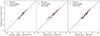 |
Fig. A.1. Star formation rate tracer (SFRHα) derived from Hα emission following the method by Duarte Puertas et al. (2017) and compared with different SFR tracers for the CO-VG sample. Left: SFRNUV + MIR following the prescription in Janowiecki et al. (2017). Centre: SFRMIR following the prescription in Leroy et al. (2019). Right: SFRHα − MPA from the MPA-JHU catalogue. |
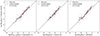 |
Fig. A.2. Star formation rate tracer (SFRHα) derived from Hα emission following the method by Duarte Puertas et al. (2017) and compared with different SFR tracers for the comparison sample. Left: SFRNUV + MIR following the prescription in Janowiecki et al. (2020). Centre: SFRMIR following the prescription in Leroy et al. (2019). Right: SFRHα − MPA from the MPA-JHU catalogue. |
We found a strong correlation between SFRNUV + MIR and SFRHα. The correlation between SFRHα and SFRMIR is good, but weaker than the previous one, particularly at low SFR values for the CO-VG sample and at high SFR values for the CO-CS sample. Finally, the correlation between SFRHα and SFRHα − MPA is very good for CO-VG. However, SFRHα is systematically higher than SFRHα − MPA for CO-CS galaxies, especially at lower SFR values. This is in agreement with the previous results of Duarte Puertas et al. (2017) and Domínguez-Gómez et al. (2022). In conclusion, the SFRHα tracer appears to yield very similar results to the SFRNUV + MIR tracer (the mean difference between the values of SFRNUV + MIR and SFRHα is 0.01 dex for the CO-VG sample and 0.02 for CO-CS) over almost 3 orders of magnitudes. We therefore use SFRHα for the CO-VG sample and SFRNUV + MIR for CO-CS [defined as SFRbest in][]janowiecki17.
All Tables
L′CO10, obs luminosity, αco, molecular gas mass, and aperture correction factor for the CO-VG sample.
Star formation rate for CO-VG and CO-CS galaxies: Mean values for galaxies on the SFMS.
Molecular gas mass fraction for CO-VG and CO-CS galaxies: Mean values for galaxies on the SFMS.
Star formation efficiency for CO-VG and CO-CS galaxies: Mean values for galaxies on the SFMS.
All Figures
|
Fig. 1. BPT diagnostic diagram for CO-VG galaxies (left) and CO-CS galaxies (right). Blue points represent star-forming galaxies, green points represent composite galaxies, and red points represent AGN galaxies. The dashed line represents the demarcation proposed by Kewley et al. (2001), while the solid line corresponds to the curve introduced by Kauffmann et al. (2003a). |
| In the text | |
|
Fig. 2. Normalised histograms for the CO-VG (red) and the CO-CS (blue) to compare, from top to the bottom, the redshift, the stellar masses, and the sizes (R90, r, in arcsec and in kpc) of the galaxies in the two samples. |
| In the text | |
|
Fig. 3. Specific star formation rate as a function of stellar mass for the CO-VG sample (left) and the CO-CS sample (right). The SFMS is represented as a solid black line, and was derived as in Janowiecki et al. (2020, their Eq. 1). The dashed black lines represent the ±0.3 dex offset to the SFMS (Janowiecki et al. 2020) and the brown solid line represents the threshold of the RS, as also defined by Janowiecki et al. (2020, SFMS < 1.55 dex). Galaxies are colour coded according to their positions on the SFMS: (i) pink stars represent SB galaxies that lie above the SFMS, (ii) blue dots are SF galaxies within the SFMS (±0.3 dex), (iii) green diamonds are galaxies that lie in the TZ, and (iv) orange squares show RS galaxies below the TZ (SFMS < 1.55 dex). The mean sSFR per M⋆ bin is shown with a blue dashed line for the CO-VG and blue solid line for the CO-CS considering only those galaxy that belong to the SFMS. The extent of this line represents the width of the stellar mass bin. The error on the mean value is represented with a grey shadow. |
| In the text | |
|
Fig. 4. Molecular gas mass fraction as a function of stellar mass for the CO-VG sample (left) and the CO-CS sample (right). The H2MS from Janowiecki et al. (2020) is represented as a solid black line. The dashed black lines represent the ±0.2 dex offset to the H2MS. Galaxies are colour coded according to their positions on the SFMS as described in Fig. 3. The mean logarithm of the molecular gas mass fraction per M⋆ bin is shown with a blue dashed line for the CO-VG and a blue solid line for the CO-CS considering only those galaxies that belong to the SFMS. The extent of this line represent the width of the stellar mass bin. The error of the mean value is represented with a grey shadow. The MH2 upper limits are represented with downward-pointing arrows. |
| In the text | |
|
Fig. 5. Histograms of ΔH2MS for the CO-VG sample (left) and the comparison sample (right). The three categories of galaxies are colour coded with respect to their positions on the SFMS; (i) pink for SB galaxies above the SFMS, (ii) blue for SF galaxies within the SFMS (±0.3 dex), and (iii) green for galaxies that lie in the TZ. H2 detections are shown as full lines and non-detections as dotted histograms. |
| In the text | |
|
Fig. 6. ΔSFMS as a function of ΔH2MS for the CO-VG sample (left) and the comparison sample (right). Galaxies are colour coded according to their position on the SFMS as described in Fig. 3. The blue and orange lines represent fits for the CO-VG sample and the comparison sample, respectively. The respective blue and orange shadows represent the 1σ dispersion of the fits. The CO non-detections are shown with leftward-pointing arrows. |
| In the text | |
|
Fig. 7. Star formation efficiency as a function of stellar mass for the CO-VG sample (left) and the CO-CS (right) sample. Galaxies are colour coded according to their position on the SFMS as described in Fig. 3. The mean logarithm of the SFE per M⋆ bin is shown with a blue dashed line for the CO-VG and a blue solid line for the CO-CS sample, considering only those galaxies that belong to the SFMS. The extent of this line represent the width of the stellar mass bin. The error of the mean value is represented with a grey shadow. The lower limits are shown with upward-pointing arrows. |
| In the text | |
|
Fig. 8. Star formation efficiency as a function of SFMS distance for the CO-VG sample (left) and the comparison sample (right). Galaxies are colour coded according to their position on the SFMS as described in Fig. 3. The blue and orange lines represent fits for the CO-VG sample and the comparison sample, respectively, considering the four categories of galaxies. The respective blue and orange shadows represent the 1σ dispersion of the fits. The black thick line represents the power law found by Tacconi et al. (2018). |
| In the text | |
|
Fig. 9. ICO(2 − 1) and ICO(1 − 0) line emission (on the Tmb temperature scale) for the CO-VG sample and the CO-CS sample. To guide the eye, we include lines for fixed ratios between ICO(2 − 1) and ICO(1 − 0). |
| In the text | |
|
Fig. 10. Observed line-intensity ratio R21 = ICO(2 − 1)/ICO(1 − 0) as a function of the r-Petrosian R90, r. Left panel: Only detections and upper limits (i.e. data points with non-detections in ICO(1 − 0) were not considered). Right panel: Only detections and lower limits (i.e. data points with non-detections in ICO(2 − 1) were not considered. |
| In the text | |
|
Fig. A.1. Star formation rate tracer (SFRHα) derived from Hα emission following the method by Duarte Puertas et al. (2017) and compared with different SFR tracers for the CO-VG sample. Left: SFRNUV + MIR following the prescription in Janowiecki et al. (2017). Centre: SFRMIR following the prescription in Leroy et al. (2019). Right: SFRHα − MPA from the MPA-JHU catalogue. |
| In the text | |
|
Fig. A.2. Star formation rate tracer (SFRHα) derived from Hα emission following the method by Duarte Puertas et al. (2017) and compared with different SFR tracers for the comparison sample. Left: SFRNUV + MIR following the prescription in Janowiecki et al. (2020). Centre: SFRMIR following the prescription in Leroy et al. (2019). Right: SFRHα − MPA from the MPA-JHU catalogue. |
| In the text | |
Current usage metrics show cumulative count of Article Views (full-text article views including HTML views, PDF and ePub downloads, according to the available data) and Abstracts Views on Vision4Press platform.
Data correspond to usage on the plateform after 2015. The current usage metrics is available 48-96 hours after online publication and is updated daily on week days.
Initial download of the metrics may take a while.