| Issue |
A&A
Volume 690, October 2024
|
|
|---|---|---|
| Article Number | A302 | |
| Number of page(s) | 16 | |
| Section | Extragalactic astronomy | |
| DOI | https://doi.org/10.1051/0004-6361/202451432 | |
| Published online | 18 October 2024 | |
Charting the Lyman-α escape fraction in the range 2.9 < z < 6.7 and consequences for the LAE reionisation contribution
1
Aix Marseille Université, CNRS, CNES, LAM (Laboratoire d’Astrophysique de Marseille), UMR 7326, 13388 Marseille, France
2
Department of Astrophysics, Vietnam National Space Center, Vietnam Academy of Science and Technology, 18 Hoang Quoc Viet, Hanoi, Vietnam
3
Graduate University of Science and Technology, VAST, 18 Hoang Quoc Viet, Cau Giay, Vietnam
4
Institute of Science and Technology Austria (ISTA), Am Campus 1, 3400 Klosterneuburg, Austria
5
Centre for Astrophysics and Supercomputing, Swinburne University of Technology, Hawthorn, VIC 3122, Australia
6
Leibniz Institut für Astrophysik (AIP), An der Sternwarte 16, 14482 Potsdam, Germany
Received:
9
July
2024
Accepted:
13
July
2024
Abstract
Context. The escape of Lyman-α photons at redshifts greater than two is an ongoing subject of study and an important quantity to further understanding of Lyman-α emitters (LAEs), the transmission of Lyman-α photons through the interstellar medium and intergalactic medium, and the impact these LAEs have on cosmic reionisation.
Aims. This study aims to assess the Lyman-α escape fraction, fesc, Lyα, over the redshift range 2.9 < z < 6.7, focusing on Very Large Telescope/Multi Unit Spectroscopic Explorer (VLT/MUSE) selected, gravitationally lensed, intrinsically faint LAEs. These galaxies are of particular interest as the potential drivers of cosmic reionisation.
Methods. We assessed fesc, Lyα in two ways: through an individual study of 96 LAEs behind the A2744 lensing cluster, with James Webb Space Telescope/Near-Infrared Camera (JWST/NIRCam) and HST data, and through a study of the global evolution of fesc, Lyα using the state-of-the-art luminosity functions for LAEs and the UV-selected ‘parent’ population (dust-corrected). We compared these studies to those in the literature based on brighter samples.
Results. We find a negligible redshift evolution of fesc, Lyα for our individual galaxies; it is likely that it was washed out by significant intrinsic scatter. We observed a more significant evolution towards higher escape fractions with decreasing UV magnitude and fit this relation. When comparing the two luminosity functions to derive fesc, Lyα in a global sense, we saw agreement with previous literature when integrating the luminosity functions to a bright limit. However, when integrating using a faint limit equivalent to the observational limits of our samples, we observed enhanced values of fesc, Lyα, particularly around z ∼ 6, where fesc, Lyα becomes consistent with 100% escape. This indicates for the faint regimes we sampled that galaxies towards reionisation tend to allow very large fractions of Lyman-α photons to escape. We interpret this as evidence of a lack of any significant dust in these populations; our sample is likely dominated by young, highly star-forming chemically unevolved galaxies. Finally, we assessed the contribution of the LAE population to reionisation using our latest values for fesc, Lyα and the LAE luminosity density. The dependence on the escape fraction of Lyman continuum photons is strong, but for values similar to those observed recently in z ∼ 3 LAEs and high-redshift analogues, LAEs could provide all the ionising emissivity necessary for reionisation.
Key words: galaxies: evolution / galaxies: formation / galaxies: luminosity function / mass function / galaxies: starburst
Corresponding authors; This email address is being protected from spambots. You need JavaScript enabled to view it. ; This email address is being protected from spambots. You need JavaScript enabled to view it.
© The Authors 2024
 Open Access article, published by EDP Sciences, under the terms of the Creative Commons Attribution License (https://creativecommons.org/licenses/by/4.0), which permits unrestricted use, distribution, and reproduction in any medium, provided the original work is properly cited.
This article is published in open access under the Subscribe to Open model. This email address is being protected from spambots. You need JavaScript enabled to view it. to support open access publication.
1. Introduction
For more than 20 years, the study of high-redshift galaxies has been facilitated by the Lyman-α line (Cowie & Hu 1998; Hu et al. 1998). Galaxies for which this line is observable, Lyman-α emitters (LAEs; equivalent width,  ), have formed an essential part of the drive to characterise star-forming galaxies (SFGs) at increasingly higher redshifts (the most recent examples include, Witstok et al. 2024b; Iani et al. 2023; Chen et al. 2024, see also Ferrara 2024 and references therein). The Lyman-α line, while intrinsically very strong and therefore an attractive target for observations, undergoes a very complicated process escaping a galaxy due to the resonant nature of the line (Verhamme et al. 2008; Hayes et al. 2010; Zheng et al. 2010; Dijkstra & Kramer 2012; Matthee et al. 2016b) as well as dust within the galaxy (Atek et al. 2008; Finkelstein et al. 2009; Hayes et al. 2013), inflows and outflows (Hansen & Oh 2006; Gronke & Dijkstra 2016), and the intergalactic medium (IGM) (Stark et al. 2010, 2011). Understanding the escape of these Lyman-α photons is of paramount importance to the characterisation of these high-redshift SFGs as well as to understanding their impact on extragalactic processes such as cosmic reionisation.
The escape of Lyman-α photons is also expected to be connected to the escape of ionising Lyman continuum photons ( ) (Dijkstra et al. 2016; Verhamme et al. 2017; Steidel et al. 2018; Izotov et al. 2022; Yuan et al. 2024; Choustikov et al. 2024a; Pahl et al. 2024; Gazagnes et al. 2024), although any relation between these two photon escapes tends to be reported with significant scatter between individual galaxies. Since the escape of Lyman continuum photons is extremely challenging to observe directly at redshifts higher than z ∼ 3 due to the intervening IGM, the escape of Lyman-α photons can be an important proxy.
Many efforts have been made towards a better understanding, both on the theoretical and observational front, and a better quantification of the escape fraction (henceforth fesc, Lyα). The well-known relations in Kennicutt (1998a) quantify the basic relationship between Lyman-α luminosity and the star-formation rate (SFR) expected to produce it, subject to assumptions on the initial mass function (IMF), stellar metallicity, and star-formation history (SFH). However, the resonance of the Lyman-α line means that Lyman-α photons will scatter in a galaxy’s neutral hydrogen. During this process, dust may absorb these photons (Schaerer & Verhamme 2008; Ciardullo et al. 2014; Dijkstra 2016 and references therein), so the Lyman-α escape fraction is expected to decrease with increasing dust content (Atek et al. 2008; Runnholm et al. 2020). The size and stellar mass of galaxies may also play a role, with fesc, Lyα generally increasing with lower stellar mass (Oyarzún et al. 2017; Yang et al. 2017; Goovaerts et al. 2024).
The increasing neutrality of the IGM at redshifts above z ∼ 5 − 6 (McGreer et al. 2018; Planck Collaboration VI 2020) is expected to play a significant role in Lyman-α visibility. Neutral hydrogen around the galaxy and along the line of sight absorbs Lyman-α emission, meaning that the number density of LAEs decreases around these redshifts (Schaerer et al. 2011; Pentericci et al. 2011; De Barros et al. 2017; Arrabal Haro et al. 2018; Pentericci et al. 2018). However, this effect is subject to significant uncertainties, and for individual cases, it is highly dependant on the physical conditions and environment of the galaxy in question (Goovaerts et al. 2023; Witten et al. 2024).
Despite these challenges, strides have been made in recent years towards quantifying fesc, Lyα and its evolution with redshift. Blanc et al. (2011), henceforth B11, studied the evolution of dust properties and fesc, Lyα across a sample of ∼100 blank-field LAEs in the range 1.9 < z < 3.8 and compared star-formation rate densities (SFRDs) derived from LAE and UV luminosity functions (henceforth LFs) in order to quantify the evolution of fesc, Lyα with redshift. They found a sample median of ∼29% when considering their LAEs individually and a negligible redshift evolution.
Hayes et al. (2011) found a significantly lower fesc, Lyα, around 5% at z = 2.2 using a blind narrow-band survey searching for Hα and Lyman-α. The authors made use of the Hα line to estimate un-obscured star formation and compared this to the star formation derived from Lyman-α. The Hα line originates from the same process as the Lyman-α line and is less sensitive to dust attenuation; therefore, it is often a more reliable indicator of star formation.
One general agreement in the literature is that fesc, Lyα increases with redshift. Low values such as 0 − 5% are found in the aforementioned study as well as Hayes et al. (2013), Verhamme et al. (2017), Sobral et al. (2017), Sobral & Matthee (2019), and Runnholm et al. (2020). Larger values such as 30 − 40% and even higher have been found at redshifts towards the epoch of reionisation (B11; Hayes et al. 2011; Chen et al. 2024; Witstok et al. 2024a; Lin et al. 2024; Napolitano et al. 2024).
Another general agreement found in the literature relates to sample selection. Samples that are selected by their Lyman-α emission typically display higher values of fesc, Lyα when compared to samples selected by Hα (Song et al. 2014; Trainor et al. 2016; Sobral & Matthee 2019; Matthee et al. 2021).
By contrast, significant scatter in fesc, Lyα is expected in all samples, likely due to the large number of factors that affect Lyman-α photon escape and the differing conditions present in any sample of galaxies. This can be seen in all studies on fesc, Lyα, from low redshift (Hayes et al. 2010, 2013; Ciardullo et al. 2014; Matthee et al. 2016b; Runnholm et al. 2020) to the higher redshift, such as B11, Chen et al. (2024), Lin et al. (2024), and Napolitano et al. (2024).
Currently, the most powerful estimators for determining fesc, Lyα in an indirect manner include EWLyα (Sobral & Matthee 2019) and Lyman-α line separation (Yang et al. 2017; Matthee et al. 2021). The correlation with Lyman-α line separation is likely due to the presence of outflows, to which the Lyman-α line shape is sensitive (Gronke & Dijkstra 2016; Blaizot et al. 2023). These outflows produce channels of low HI column density in the interstellar medium (ISM) and circumgalactic medium (CGM), which allows for more Lyman-α escape (Hashimoto et al. 2015).
We can also constrain fesc, Lyα in a global way by comparing the SFRDs derived from the LAE and general UV-selected populations (with SFR derived from the UV emission). The ratio of these gives the escape fraction of Lyman-α photons over a specific survey volume. Employing this method, Konno et al. (2016), B11 and Hayes et al. (2011) found a gentle evolution over their redshift ranges that could be fitted with a power law of the form: fesc, Lyα = C × (1 + z)ξ, where 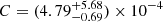 ,
,  at z ∼ 2.2 − 6.7 (Hayes et al. 2011),
 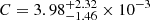 , ξ = 2.2 ± 0.3 at z = 1.9 − 3.8 (B11) and C = 5.0 × 10⁻⁴, ξ = 2.8 in z = 0 − 6 (Konno et al. 2016).
Hayes et al. (2011) mentioned that fesc, Lyα may reach unity at  , while Cassata et al. (2011) argued that fesc, Lyα would reach unity around a redshift of six. In general, such research has been done with a few LAEs fainter than log LLyα [erg/s] < 40, hence without the ability to fully constrain the faint part of the LAE LF and its impact on the SFRD.
Any difference in the evolution of fesc, Lyα may come from the integration limits during the estimation of the Lyman-α and UV luminosity densities. Hence, data on the fainter luminosity regime is necessary in order to integrate to fainter luminosity limits and better understand these faint populations’ effect on the evolution of the LF as well as fesc, Lyα with redshift.
Fortunately, the recent VLT/Multi Unit Spectroscopic Explorer (MUSE) observations of lensing clusters (Claeyssens et al. 2022; Thai et al. 2023) and blank fields (Vitte et al. 2024) have allowed us to observe Lyman-α down to log LLyα [erg/s] ∼ 39, 39.5, respectively.
In this paper, we seek to combine two state-of-the-art LFs of intrinsically faint lensed galaxies, the latest UV LF from Bouwens et al. (2022) and the latest LAE LF from Thai et al. (2023), allowing us to compare the SFRD derived from Lyman-α emission, SFRDLyα, to the total SFR density, SFRDtotal, and hence track the redshift evolution of fesc, Lyα over a wide redshift range: 2.9 < z < 6.7. In Hayes et al. (2011), the independent LF comparison is advocated as a method to calculate fesc, Lyα, though it is subject to cosmic-variance related errors. We can significantly reduce the uncertainties related to cosmic variance by using six lensing clusters for the UV LF and 17 lensing clusters for the LAE LF. The LFs we used provide this study with a unique opportunity to explore the faint galaxy regime (MUV < −13 and log LLyα [erg/s]> 39) without the need for extrapolation in the LFs.
We also calculated fesc, Lyα on an object-per-object basis in order to compare galaxy properties as well as the global fesc, Lyα evolution, based on spectral energy distribution (SED) fitting of HST and JWST/NIRCam data of ∼100 LAEs in the A2744 lensing cluster. The NIRCam data, extending to ∼5 μm, allowed us to access, for the first time, the rest-frame optical emission of these LAEs and greatly improves the reliability of the properties extracted with SED fitting. The NIRCam imaging notably also covers the entire MUSE field of view, meaning the full sample size of MUSE LAEs can be explored. This would not be the case with calculations of SFR from Hα and dust attenuation from the Balmer decrement obtained from spectroscopy, for example from JWST/NIRSpec’s MSA mode. This would, in principle, be preferable, due to the fewer assumptions needed and our lack of photometric coverage of the infrared for our LAEs. However, samples of LAEs with Balmer line detections are rare at the redshifts concerned by this study, and sample sizes are often small. Using photometry, we could gain an appreciable sample size using just one cluster, although more would be preferable (and soon possible with the current and upcoming JWST observations).
Studies of emission lines with slit spectroscopy for these galaxies (especially lensed LAEs and therefore potentially extended sources, both by lensing and due to the extended nature of Lyman-α haloes) are not without difficulties themselves. Parts of flux can be missed in slits, especially slits as small as JWST/NIRSpec’s MSA ( to
to  ; Napolitano et al. (2024) provide a good discussion of these difficulties, see also Jung et al. 2024b), and sometimes, flux can be missed altogether, such as in Jiang et al. (2023).
Section 2 outlines the determination of fesc, Lyα for individual galaxies, describing the data and process used. In Section 3, we describe the global evolution of fesc, Lyα, the two LFs used for this calculation, and the results thereof. A comparison of the two methods to each other and to studies in the literature is presented in Section 4 along with consequences for reionisation and a discussion of the validity of comparing the UV and LAE LFs. Finally, Section 5 offers conclusions and an outlook for fesc, Lyα determination in the near future.
Throughout this paper, we adopt a value for the Hubble constant of H0 = 70 km s−1Mpc−1, and the cosmology used is ΩΛ = 0.7 and Ωm = 0.3. The adopted IMF is that of Salpeter (1955). All values of Lyman-α luminosity and absolute UV magnitude are given corrected for magnification.
2. Escape fraction of individual LAEs
2.1. Data: Combining spectroscopy and photometry
In order to perform analysis of this genre, photometry and spectroscopy of sufficient quality and depth is essential. For our purposes we combined public MUSE integral field unit (IFU) spectroscopic data (Richard et al. 2021) (094.A-0115, 095.A-0181, 096.A-0496) with the latest, deepest combination of Hubble Space Telescope (HST) and James Webb Space Telescope (JWST) photometry from the UNCOVER survey (PIs Labbé and Bezanson, JWST-GO-2561, Bezanson et al. 2022) of the lensing cluster A2744. This cluster is extremely well studied and benefits from a great number of multiple images to constrain its lens models. Below, we detail the two sets of observations and how they are used for this study.
2.1.1. MUSE IFU spectroscopy
The use of an IFU allowed us to blindly select LAEs, rather than performing spectroscopic follow-up on UV-selected targets. This ensures our sample has a simple reproducible selection function, namely Lyman-α luminosity limited. MUSE has a field of view of 1 × 1 arcmin2 and a spectral resolving power of R ∼ 3000 at λ = 808 nm (Bacon et al. 2015). Wavelength coverage ranges between 4750 Å and 9350 Å, meaning the Lyman-α line can be detected between redshifts of 2.9 and 6.7.
The A2744 lensing cluster used in this work has integration times varying between 3.5 and 7 hours. It forms part of a data release by Richard et al. (2021)1 and the LAEs used in this work are comprehensively described as part of the Lensed Lyman-α MUSE Arcs (LLAMA) Sample, in Claeyssens et al. (2022).The full process of LAE detection in MUSE data is detailed in Richard et al. (2021) and Weilbacher et al. (2020). We give an abridged version here.
Emission line sources are identified in MUSE narrow-band datacubes using the MUSELET software (Piqueras et al. 2019)2. Thereafter the Source Inspection package (Bacon et al. 2023) is used to identify line emitters as LAEs and assign redshifts. During this process, the redshift confidence of each LAE is determined, based on the emission lines seen, the shape of the Lyman-α line, ancillary HST data and lensing considerations. The confidence scale ranges from 1 for a tentative redshift attribution to 3 for a very secure redshift attribution. In this work, only sources that have been identified with redshift confidence levels of two and three are used, as well as a S/N greater than three.
The flux of these LAEs is derived using SExtractor (Bertin & Arnouts 1996) on a continuum-subtracted Narrow-Band sub-cube with a size of  . The full process is described in de La Vieuville et al. (2019).
2.1.2. HST + JWST photometry and galaxy properties
The photometric catalogues of the UNCOVER project (Weaver et al. 2023) comprise photometry in 15 bands ranging from the F435W HST filter to the F444W JWST/NIRCam filter. This gives excellent, deep coverage up to 4.4 μm, which corresponds to ∼580 nm in the rest frame at z = 6.7, the highest redshift of the MUSE LAEs. We used the catalogue optimised for faint and compact sources (0.32″ apertures). 5σ depths in the 15 filters range between 27.16 and 29.56 in AB magnitudes. Of the 154 total LAE images, 121 were detected, which corresponds to 99 individual LAEs. We rejected two of these LAEs as being clearly contaminated by bright cluster galaxies and a further LAE, as it lies on a critical line and has a magnification factor of 137 ± 1500. As such, its properties would likely not be well constrained (see, for example, Limousin et al. 2016). Having thus blindly matched these Lyman-α-selected galaxies to their UV counterparts, their SEDs were fitted with the SED-fitting code CIGALE (Boquien et al. 2019). The details of the fitting procedure are outlined in Goovaerts et al. (2024); here we give a brief outline.
Taking advantage of the secure spectroscopic redshifts of these LAEs, we fit their SEDs using two different SFHs: a single exponentially decaying burst with a range of timescales and a double burst model with a second, delayed burst at a time τ after the initial burst, to be fit (Małek et al. 2018). Ages for the bursts range from 10 to 700 Myr and mass fractions in the second burst range from 0.001 to 0.65. The stellar template library of Bruzual & Charlot (2003) is employed with metallicities ranging from 0.001 to 0.02, together with the nebular emission models from Theulé et al. (2024). Gas metallicities range between 0.0004 and 0.02. Dust attenuation is taken into account by means of the Calzetti attenuation law (Calzetti et al. 2000).
The best-fit SFH and model was carried forward in this analysis (see Goovaerts et al. 2024 for comparisons between the two SFHs). One of the parameters in the CIGALE output is the intrinsic dust-corrected star formation, which is used in the computation of fesc, Lyα.
2.1.3. Lensing models
For studies involving lensing clusters, the lens models used are pivotal to the reliability of the results, as these govern the lensing magnifications that are assigned to each galaxy and therefore the correction made to their observed luminosity. The lens models used for this work for the A2744 lensing cluster are described in Richard et al. (2021). As the Hubble Frontier Fields (HFF) and A2744 in particular have been so well studied over the years, these clusters have very well constrained mass models, drawing on many multiple images identified behind each cluster. While systematic uncertainties are still associated to the particular lens model used (Acebron et al. 2017; Furtak et al. 2021), the quantity of multiple images for these particular clusters render the statistical error on the mass distribution as low as 1% (Richard et al. 2021). Typical, accepted magnifications in the sample range from 1.5 to 25, with the maximum magnification being 137. We note that escape fraction measurements for individual galaxies (as in the following Section), are not affected by magnification.
2.2. Escape fraction
To calculate the escape fraction on an object-per-object basis for the 96 individual LAEs behind the A2744 lensing cluster, from the data described in Section 2.1, we compare the SFR inferred from the Lyman-α flux, to the dust-corrected SFR from the CIGALE SED fitting process. The SFR inferred from the Lyman-α flux is calculated using the prescription in Kennicutt (1998a) and the conversion factor of 8.7 between Lyman-α and Hα luminosities, using a Case B recombination scenario (Osterbrock 1989) (T = 104 K).
The ratio of these two SFRs gives the escape fraction of Lyman-α photons, fesc, Lyα. The redshift evolution of this quantity is shown in Fig. 1. The sample median is shown as the red dashed line and the sample median in B11 is shown as the cyan dashed line. They are consistent to within each other’s errors, even though B11 use a different prescription for finding fesc, Lyα. The median escape fraction uncertainty of our sample (18%) is shown by the black error bar. Each LAE is colour-coded by its absolute UV magnitude, calculated from the filter that sees the rest frame 1500 Å emission. One can clearly see that Lyman-α photons escape more easily from UV-fainter objects, a result already remarked upon by Lin et al. (2024), Napolitano et al. (2024). To clarify this further, we can fit a relation between the absolute UV magnitude and fesc, Lyα for each galaxy. This is shown in Fig. 2, where the galaxies are now colour-coded by redshift-bin and median error bars for each bin are shown in the corresponding colour. The best-fit to this data is
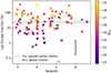 |
Fig. 1. Redshift evolution of the escape fraction of Lyman-α photons from LAEs in the A2744 lensing cluster colour-coded by the absolute UV magnitude of each LAE. The global medians of our sample and that in B11, are shown with red and cyan dashed lines respectively. The median uncertainty of the sample (∼18%) is shown by the black error bar, as if it was at the level of the global median, offset for clarity. |
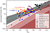 |
Fig. 2. Evolution of fesc, Lyα with absolute UV magnitude MUV. Photometrically detected galaxies are split into three redshift bins to stress the lack of evolution in this sense, while the evolution with MUV is fit by the relation in cyan (details in text). Median error bars for the three redshift bins are shown in the corresponding colour and fesc, Lyα error bars are also listed here for clarity (relevant redshift bin in brackets): 0.18 (2.9 < z < 4), 0.12 (4 < z < 5) and 0.25 (5 < z < 6.7). Absolute magnitude values and their errors are adjusted for magnification. Black triangles denote continuum-undetected LAEs. MUV values are upper limits and escape fraction values are lower limits. These objects are not included in the fit. Red shaded areas denote regions of incompleteness based on MUSE line-detections: a darker colour representing increasing lensing magnification (see text). |
 (1)
(1)
This is clearly a tighter relation than the one shown by the redshift versus fesc, Lyα, with an uncertainty on the slope and normalisation of about 10%. These quantities, MUV and fesc, Lyα are not independent as MUV is related to the intrinsic SFR of a galaxy, so this relation is to be expected, but it is nevertheless noticeable that below MUV = −18 there are few galaxies with fesc, Lyα values less than 10%. However, care must be taken when interpreting this result, as incompleteness can play a role as we start to probe fainter galaxies (towards the right of Fig. 2). To better assess this, in Fig. 2 we plot three regions where we expect to be incomplete as a function of UV magnitude and lensing magnification. This is based on the limiting flux for a MUSE detection (of an LAE). The three magnification regions plotted are μ = 1.5, the minimum magnification included in the sample (the area covered by MUSE observations do not reach the areas with less magnification than this, most of the area has μ > 2), μ = 9, the maximum magnification for an image included in the sample (we note that there are LAEs not included and images not included with μ > 9) and μ = 137, the maximum magnification of any LAE image in the A2744 lensing cluster. These three regions delineate the area of this plot where we expect to become incomplete in terms of detecting a faint galaxy with a small fesc, Lyα value with MUSE. We can see that this effect likely becomes important towards the faint end of this plot, at MUV ≳ −17. However, at the brighter end of this graph, we do not expect the incompleteness to shape the relation we observe.
We did see LAEs undetected in the continuum that might be expected to fill this region of the graph. However, they are uniquely objects of high escape fraction (based on upper limits of the UV continuum, and no dust correction). These objects are denoted by the black triangles in Fig. 2: lower limits on fesc, Lyα and upper limits on MUV.
We note also that around this MUV value of −18 that we start to see objects with fesc, Lyα > 100%. fesc, Lyα > 100% means that we are seeing more Lyman-α emission than we should, given the standard conversions between Lyman-α and UV luminosities and SFR detailed above. Reasons for this may include our assumptions in making those conversions, such as constant SFH, ages greater than ∼50 Myr and the case B recombination scenario (Osterbrock 1989), becoming less valid (see, for example, McClymont et al. 2024). This may point concurrently to our models failing to correctly estimate the dust content of these galaxies and thereby underestimating the intrinsic SFR. However, this would mean that some property of these galaxies is heavily attenuating the UV emission, but not attenuating the Lyman-α emission accordingly. Atek et al. (2008) postulate that geometry or the presence of large outflows may play a role in disconnecting Lyman-α emission and dust such that one may see a high fesc, Lyα from a heavily dust-attenuated system.
We also observed LAEs for which the continuum is completely undetected in the deepest photometry to date (Bacon et al. 2015; Maseda et al. 2020; de La Vieuville et al. 2020; Goovaerts et al. 2023; Maseda et al. 2023), and fesc, Lyα for these galaxies is, naturally, very high, often greater than 100% (as calculated from 2σ upper limits on the UV continuum). This suggests that there is more than simply model inadequacy at play here. We discuss these objects further in Section 4.
Unlike MUV, we see no significant evolution of fesc, Lyα with redshift, although we have relatively few objects at redshifts higher than 6. It is clear from Fig. 1 that we are affected by missed objects above z = 6, both in the high-fesc, Lyα regime (as these objects have low MUV) and the low-escape fraction regime, as objects with low fesc, Lyα are harder to detect at higher redshifts. The greater presence of skylines and decreased MUSE sensitivity towards longer wavelengths are additional challenges to detect LAEs towards the high end of our redshift range.
The comparison to the results in B11 suggest that fesc, Lyα does not evolve significantly over the redshift range 1.8 < z < 6. This is in tension with certain literature results such as Hayes et al. (2011), who find that fesc, Lyα increases with redshift (0.6 < z < 6). However, this study was performed in a similar way to the global analysis of fesc, Lyα that we present in the following sections. Hence, we return to this point after having taken both methods into consideration.
The scatter in the individual results shown in Fig. 1 is to be expected, given the wide variety of conditions within galaxies, even LAEs, expected to be mostly young and highly star forming. Dust content of these galaxies likely varies, which plays a significant role in the escape of Lyman-α photons (Verhamme et al. 2008). Additionally and as mentioned, geometry and line-of-sight effects are also expected to have a hand in the amount of Lyman-α photons that reach the observer (Verhamme 2012; Dijkstra & Kramer 2012; Gronke & Dijkstra 2016; Blaizot et al. 2023; Giovinazzo et al. 2024).
While we see consistency between the sample median of B11 and ours, the offset, as well as the smaller scatter of our results, is to be expected based on the differing methods for finding fesc, Lyα. B11 assume an intrinsic UV slope of −2.23 in order to calculate the dust reddening E(B − V). As this UV slope likely depends on factors other than dust, such as metallicity, age and mass of the stellar population (Buat et al. 2012; Wilkins et al. 2013; Bouwens et al. 2016; Reddy et al. 2018; Topping et al. 2022), and as there is evidence for slopes bluer than this value (De Barros et al. 2017; Naidu et al. 2022; Goovaerts et al. 2023; Iani et al. 2023; Nanayakkara et al. 2023; Napolitano et al. 2024), we prefer not to use this assumption. If there are bluer intrinsic slopes than this, we would expect the corresponding E(B − V) values from B11 to be higher, and therefore, the intrinsic SFR would be higher, and the calculated escape fractions would be lower. This is what we observed in our results. We also saw less scatter in fesc, Lyα, as we do not depend on estimations of the UV slope, which are known to have significant scatter (as well as uncertainty and possibly bias, e.g. Austin et al. 2024).
Our sample median, 22.5%, agrees with determinations at slightly lower redshift from Sobral et al. (2017), Matthee et al. (2021), who both quote escape fractions of ∼30% for LAEs. Most recently, also using JWST, Chen et al. (2024) have found a sample median of 28% for 10 LAEs at 5 < z < 8.
However, we note that the scatter on individual determinations of fesc, Lyα remains a very significant consideration when assessing samples of the kind in Fig. 1. It is therefore unlikely that we will be able to specify a precise fraction for Lyman-α escape at any given redshift. It is clear that the trend of fesc, Lyα with MUV is more useful.
We note also that while individual fesc, Lyα values are better determined using Hα fluxes and the Balmer decrement, the intrinsic scatter seen remains similar, with values ranging from < 1% escape to 100% (see, for example, Chen et al. 2024; Napolitano et al. 2024). For our sample, we can take additional encouragement from the fact that the dust content of these low-mass LAEs, at these redshifts, is both expected to be, and observed to be, very low. We therefore do not expect many cases where our SED fitting significantly underestimates the dust attenuation of a galaxy. Both methods of determining fesc, Lyα are valuable then, and a more detailed comparison between them for the same sample of galaxies is desirable.
3. Evolution of the global Lyman-α escape fraction
One can derive estimates of fesc, Lyα in a global manner by comparing the LF of LAEs and that of the ‘total’ galaxy population. Integrating both of these LFs gives the Lyman-α luminosity density ρLyα and the total luminosity density ρtotal. From this one can derive the respective SFRDs. Then taking the ratio of these SFRDs gives fesc, Lyα (Hayes et al. 2011; Blanc et al. 2011; Zheng et al. 2013; Konno et al. 2016). In order to perform this calculation, we start from the two state-of-the-art LFs in lensing fields, the LAE LF from Thai et al. (2023) and the UV LF from Bouwens et al. (2022), assumed here to be the ‘total’ galaxy population. This assumption and its consequences for the results of this study are discussed in detail in Sect. 4.3.
Before presenting the derivation of fesc, Lyα, we briefly detail both LFs used, starting with the LAE LF from Thai et al. (2023).
3.1. Lyman-α luminosity function
The LAE LF is computed by using the non-parametric Vmax method to estimate the volume of the survey in which we can detect sources individually. The inverse of this parameter is the contribution of the source to the numerical density of the galaxies. The procedure to compute this parameter using data collected by lensing observations by MUSE/VLT was developed by de La Vieuville et al. (2019) and presented in Thai et al. (2023) with some improvements related to the magnification and completeness values of the sources. These completeness values reflect the expected number of galaxies actually in the field based on the observed galaxies and the noise statistics of the field. The sample in Thai et al. (2023) includes 600 LAEs behind 17 lensing clusters observed by MUSE/VLT, identified with highly secure redshifts, zconf = 2, 3 (high Lyman-α line S/N, clearly asymmetric line profile, etc) as defined in Richard et al. (2021). These data are within a redshift interval 2.9 < z < 6.7 and covering four orders of magnitude in luminosity 39 < log L [erg s−1]< 43. These luminosity values were corrected for the magnification of the lensing effect using models from the work of Pello et al. (1991), Covone et al. (2006), Richard et al. (2010), Mahler et al. (2018), Lagattuta et al. (2019), Beauchesne et al. (2023), Richard et al. (2021).
The evolution of the LF with redshift was investigated in four redshift intervals 2.9 < z < 6.7, 2.9 < z < 4.0, 4.0 < z < 5.0 and 5.0 < z < 6.7 (labelled zall, z35, z45 and z56) and the Schechter function used to fit the LF points. Using the data sample collected with the help of gravitational lensing is efficient to study the LF at faint Lyman-α luminosities (log L [erg s−1] < 41). However, it becomes less sensitive when examining the function surrounding the characteristic luminosity value L* of the Schechter function. To tackle this problem, Thai et al. (2023) used the average LF values obtained from the literature in the same luminosity and redshift bins as a constraint at the bright end of the LF. A turnover in the shape of the LF was observed at luminosities log L [erg s−1] < 41 when studying the evolution in the z45 and z56 redshift intervals. This was explained by inefficient cooling of gas in small dark matter haloes (Jaacks et al. 2013; Gnedin 2016; Yue et al. 2016). To accommodate the potential turnover in these two redshift bins, a modified Schechter function was introduced by multiplying an exponential term exp − (LT/L)m to the traditional Schechter function. The best-fit results suggest that m is about unity and log LT [erg s−1] is ∼40 and ∼40.7 for the redshift intervals z45 and z56 respectively. Accounting for the effects of source selection, completeness cut, and flux measurement, the final slope values in the four redshift intervals are −2.00 ± 0.50, −1.97 ± 0.50, −2.28 ± 0.50 and −2.06 ± 0.60. These values are in good agreement with results from other literature studies within a 1σ deviation. The best-fit value of the characteristic luminosity values are log L* [erg s−1] =  ,
,  ,
,  ,
,  and the normalisation factors are ϕ * [10−4 Mpc−3] =
  ,
,  ,
,  and
and  in redshift bins zall, z35, z45 and z60, respectively.
In our analysis we also include results for the LAE LF at different redshift intervals from literature studies to build a general picture, and provide brief descriptions of these works here. de La Vieuville et al. (2019) studied the LF evolution of ∼120 LAEs behind four lensing clusters observed by MUSE, with the same redshift range as Thai et al. (2023) and a luminosity range of 39 ≲ log LLyα[erg/s]≲43. In the blank field observations, Ouchi et al. (2008), Blanc et al. (2011), Cassata et al. (2011), Drake et al. (2017), Konno et al. (2016) presented the LF evolution with redshift of LAEs with luminosities greater than log L [erg/s] = 41. Due to lacking data at faint luminosities, Ouchi et al. (2008) fixed the slope value of the Schechter function at α = −1.5 (z = 3.1, 3.7, 5.7). B11 fixed this parameter at α = −1.7 (z = 1.9 − 3.8), while Cassata et al. (2011) found 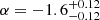 ,
,  , −1.69 (fixed) at z = 1.95 − 3.0, 3.0 − 4.55, 4.55 − 6.6, respectively. However, at a higher redshift and a brighter luminosity range, this value has been found to be much steeper, varying from −2.26 to −2.56 at redshift z = 5.7, and from −1.86 to −2.5 at redshift z = 6.6 (Konno et al. 2016); or ∼ − 1.98 at redshift z = 5.4 ± 0.4 (Sobral et al. 2018), depending on the luminosity limitations used for fitting.
3.2. Ultraviolet luminosity function
Bouwens et al. (2022) presented a new derivation of the UV LF in the redshift range 2.0 < z < 9.0 including over 2500 lensed galaxies behind the HFF clusters using HST observations from the HFF (Lotz 2017), Grism Lens-Amplified Survey from Space (GLASS) (Treu et al. 2015) and Cluster Lensing And Supernova survey with Hubble (CLASH) (Postman et al. 2012) programmes. This LF probes down to MUV < −16 over the full redshift range we are considering in this study. A smooth flattening of α was found, from α = −2.28 ± 0.10 at redshift z = 9 to α = −1.53 ± 0.03 at redshift z ≈ 2. Over our redshift range, 3 ≲ z ≲ 7, the faint-end slope is found to evolve from α ∼ −1.60 to α ∼ −2.05. The shape of the LF and its evolution agrees well with other results in the literature, including determinations from blank fields (see Parsa et al. 2016, as well as other references in Bouwens et al. 2022).
We treat this LF as the LF of the total “parent” population in order to calculate the total SFRD. In this way, inclusive of completeness corrections, we assume that both LFs represent the “total” of their respective populations within the quoted Lyman-α luminosity and absolute UV magnitude limits. This is an assumption that we return to and discuss in Section 4.3.
All LFs, UV and LAE, are shown on a common scale (SFR) in Fig. 3. The LFs of Thai et al. (2023) and Bouwens et al. (2022) are highlighted in thicker, solid lines.
 |
Fig. 3. Ultraviolet and LAE LFs included in our analysis on a common x-axis of SFR. The LFs of Bouwens et al. (2022) and Thai et al. (2023) are shown in bold and the literature LFs are shown in coloured dash-dotted lines. The LF integration limits in terms of L* that we use throughout this work are denoted by the pink shaded regions. Left: Results from the redshift range 3 to 4. Right: Results from the redshift range 5 to 6. The literature LFs in the graph are shown in shorthand in the caption and here in full, in order: Ouchi et al. (2008), Cassata et al. (2011), Sobral et al. (2018), Thai et al. (2023), Drake et al. (2017), Bouwens et al. (2022, 2009). |
3.3. Global evolution results
The results from the Lyman-α LF in each redshift interval are integrated with luminosity to map out the evolution of Lyman-α luminosity density with redshift:
 (2)
(2)
This is then converted to the Lyman-α SFRD based on the calibration of Kennicutt (1998a), assuming the factor of 8.7 between intrinsic Lyman-α and Hα flux and a case B recombination (Osterbrock 1989):
![Mathematical equation: $$ \begin{aligned} \mathrm {SFRD}_{Ly\alpha } [M_{\odot } yr^{-1} Mpc^{-3}] = 7.9 \times 10^{-42} \times \rho _{Ly\alpha } / 8.7 . \end{aligned} $$](/articles/aa/full_html/2024/10/aa51432-24/aa51432-24-eq22.gif) (3)
(3)
The UV luminosity density is converted into the equivalent SFRD using the form SFRD = κ × ρUV (Madau & Dickinson 2014), in which κ is the conversion factor, sensitive to the recent SFH, metal-enrichment history and the IMF. The term ρUV is the UV luminosity density, which is expressed in units of erg s−1Hz−1, estimated by integration the UV LF with MUV. The widely used value of the conversion factor from Kennicutt (1998b) is κ = 1.4 × 10⁻²⁸ , where a Salpeter IMF (Salpeter 1955) is assumed. Bouwens et al. (2022) used a Chabrier IMF (Chabrier 2003) for this conversion, so we correct for this, using a factor of 1.96. Going forward, the SFRD obtained from UV LF is treated as the total SFRD of the entire galaxy population. We estimated the total UV SFRD down to MUV = −13 at redshifts z = 2, 3, 4, 5, 6, 7 (see Table 1 for the values used, after correction to the Salpeter IMF). Subsequently we interpolated the SFRD to redshifts z = 2.5, 3.1, 3.5, 3.7, 4.5, 4.7,5.4, 5.7 to adapt to redshift bins used in the literature studies.
Ultraviolet SFRD used to calculate fesc, Lyα.
The ratio between the LAE SFRD and the total, dust-corrected SFRD in a given redshift interval gives the global Lyman-α escape fraction. This definition was applied in the works of Hayes et al. (2011), Cassata et al. (2011), B11, Zheng et al. (2013) and Konno et al. (2016). The results for the global escape fraction derived in this work are shown in Figs 4 and 5. We compared our results to the results derived using several LAE LFs in the literature, for which we adopted an identical approach to that described above (Ouchi et al. 2008; Blanc et al. 2011; Cassata et al. 2011; de La Vieuville et al. 2019; Thai et al. 2023; Sobral et al. 2018). We used the same UV LF for each comparison.
 |
Fig. 4. Global redshift evolution of fesc, Lyα with an integration limit on both LFs of 0.04L*. Our results, using the LFs from Thai et al. (2023) are shown in cyan for the modified Schechter function and pink for the general Schechter function. The dotted horizontal line denotes fesc = 100%. The dash-dotted green curve is from Hayes et al. (2011) in the redshift range of 2.2 − 6.6 and calculated with the integration limit 0.04L*. The red dash-dotted curve is the best fit to all the data shown and the blue dash-dotted curve fits just the data of Thai et al. (2023) (cyan points: modified Schechter function). |
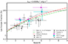 |
Fig. 5. Global redshift evolution of fesc, Lyα with an integration limit on both LFs of 0.0006L*. Results from this study are shown by cyan (modified Schechter function) and pink (general Schechter function) points. Power-law fits from the literature are shown in grey and green (B11, Hayes et al. 2011) and the equivalent fit to all the data is shown in red. The fit from Hayes et al. (2011) is derived from results integrated to 0.04L*, and the fit from B11 from results integrated to 0. |
The lower limits of the respective LF integrations are worth noting. We used two different limits, the first was 0.04L* and the second was 0.0006L* (where L* is the characteristic galaxy luminosity of the Schechter function). The first limit, as suggested in Hayes et al. (2011) is designed to compare our study to previous results using brighter galaxies. It corresponds to limits of ![Mathematical equation: $ {\log\,L_{\mathrm{Ly\alpha}} [\text{ erg} \, \text{ s}^{-1}]\sim41} $](/articles/aa/full_html/2024/10/aa51432-24/aa51432-24-eq23.gif) and MUV ∼ −17 respectively. The results for fesc, Lyα calculated with this limit are shown in Fig. 4. The second limit, 0.0006L*, corresponds to the faint regimes that we reach with the LAE and UV LFs (
and MUV ∼ −17 respectively. The results for fesc, Lyα calculated with this limit are shown in Fig. 4. The second limit, 0.0006L*, corresponds to the faint regimes that we reach with the LAE and UV LFs (![Mathematical equation: $ {\log\,L_{\mathrm{Ly\alpha}}[\text{ erg} \, \text{ s}^{-1} ]\sim39.5} $](/articles/aa/full_html/2024/10/aa51432-24/aa51432-24-eq24.gif) and MUV ∼ −13) and is shown in Fig. 5. The vertical error bars are estimated from published uncertainty values in ϕ*, α, L* (LAE LFs) and ϕ*, α, M* (UV LF). The horizontal error bars display the redshift intervals of each survey. As de La Vieuville et al. (2019) and Thai et al. (2023) probed the LAE LF at the same redshift intervals, the data points derived from the LF of de La Vieuville et al. (2019) have been shifted by 0.1 in redshift. Table A.1 presents the results for each study using this integration limit, as well as the SFRD value derived. By comparing the results obtained with the different limits we can assess the impact of the faint galaxies that we reach with the latest LAE and UV LFs.
and MUV ∼ −13) and is shown in Fig. 5. The vertical error bars are estimated from published uncertainty values in ϕ*, α, L* (LAE LFs) and ϕ*, α, M* (UV LF). The horizontal error bars display the redshift intervals of each survey. As de La Vieuville et al. (2019) and Thai et al. (2023) probed the LAE LF at the same redshift intervals, the data points derived from the LF of de La Vieuville et al. (2019) have been shifted by 0.1 in redshift. Table A.1 presents the results for each study using this integration limit, as well as the SFRD value derived. By comparing the results obtained with the different limits we can assess the impact of the faint galaxies that we reach with the latest LAE and UV LFs.
To investigate the global evolution of escape fraction with redshift, we recall the power-law form that was proposed by B11 and Hayes et al. (2011):  . The coefficient C is constrained strongly by the evolution of escape fraction at low redshift while the exponent ξ is defined by the evolution at high redshift. In Fig. 4, the best fits calculated for this work are shown as red and blue dash-dotted lines, fitting all the points in the graph and only those of Thai et al. (2023), respectively. In Fig. 5, the red fit is to all the data. The green dashed line shows the fit from Hayes et al. (2011), which used the UV LF obtained from Ouchi et al. (2004), Reddy et al. (2008), Bouwens et al. (2009) and an LF integration down to 0.04L* (fitted to data over the range 2 < z < 6). We leave this fit in both plots to guide the eye as to the difference when integrating to a fainter limit. B11 use the results of Bouwens et al. (2010) and an integration limit of 0. The fit of B11 is shown in Fig. 5 to provide the comparison to earlier results which have been integrated to 0.
We find C = 14.3 ± 14.0 × 10⁻⁴ and ξ = 2.3 ± 0.6 when fitting to all the literature and C = 12 ± 43 × 10−4 and ξ = 2.8 ± 2.1 when only fitting the results from Thai et al. (2023) with the integration limit at 0.04L*. With the lower integration limit of 0.0006L*, we find C = 4.1 ± 7.7 × 10⁻⁴ and ξ = 3.6 ± 1.2 when fitting our results together with all the ancillary data in Fig. 5. Because the other studies included in this graph do not probe the faint regime that our LFs do (equivalent to the integration limit of 0.0006L*), and they therefore require an extrapolation outside the limits of the datasets used. During this fitting process, we set the weight of each point equal to the weight of the equivalent point from our study (i.e. the cyan point in the same redshift bin). This relation is qualitatively consistent with the equivalent relation derived in Hayes et al. (2011) (green dashed line, noting that this relation is derived using a different UV LF and a brighter integration limit) and suggests that fesc, Lyα will reach 100% around z = 8.
4. Discussion
With the individual and global results now in hand, we can compare them and consider what these can tell us about fesc, Lyα and its evolution.
4.1. Global fesc, Lyα evolution
Fig. 4 shows the determination of fesc, Lyα using the LF integration limit 0.04L*. We plotted this graph in order to compare our results to previous literature determinations of the escape fraction, which used samples of galaxies brighter than this work, and to assess the impact of the bright (MUV < −17) and faint populations (MUV < −13) on the evolution of fesc, Lyα. We plotted results derived using both the modified (cyan) and the general Schechter (pink) functions in order to show the difference in these results created by the presence or lack of a turnover in the LAE LF. However, at this integration limit, the behaviour of the modified Schechter function is close to that of the traditional Schechter function, so we did not see a significant difference in SFRDLyα. As the current best derivations of the LF come from the modified Schechter functions, going forth we discuss the results related to these (cyan points).
We observed a good agreement at all redshifts between the results derived in this work and the results from the literature. We saw little evolution between z ∼ 3.5 and z ∼ 4.5, followed by a jump in fesc, Lyα at z ∼ 6, but at each redshift, our results agree well with the established literature. When fitting our data (blue line) compared to all the results (red line), we observed an enhancement of fesc, Lyα, likely due to the constraints placed by the literature in the redshift range 2 < z < 4. Our points do lie systematically above the points from the literature, indicating a greater SFRD based on the latest LAE LF of Thai et al. (2023). We note, however, that the LFs of Konno et al. (2016) and Drake et al. (2017) have not been included in Figs. 4 and 5 due to large uncertainties, especially at the highest redshifts and faint luminosities. These uncertainties contribute to unrealistically high (and poorly constrained) escape fractions based on these LFs.
Additionally, the choice of completeness cut has an impact. In Thai et al. (2023), a completeness cut of 1% was chosen (i.e. LAEs with completeness values < 1% are not taken into account in the LF determination), in order to maximise the sample size, while still negating the effect of the most incomplete and therefore uncertain sources. Studies have typically chosen different completeness cuts, or none at all. For example, de La Vieuville et al. (2019) chose 10%, rejecting a larger number of sources. In order to check the effect this has, we recomputed fesc, Lyα using the LF cut at 10% completeness. This yielded values similar to those seen in the literature: 10 − 15% escape. Therefore, we consider our results completely consistent with what has been found previously when considering a brighter integration limit (0.04L*).
The green dashed fit of Hayes et al. (2011) lies slightly higher than the literature data. We attribute this to the significant update in the UV LF since the publishing of that study (the UV LFs of Bouwens et al. (2009) and Reddy et al. (2008) were used for this fit). This emphasises the importance of the UV LF in these calculations and the value of the latest determination from Bouwens et al. (2022). The values used in this work, inclusive of dust and IMF correction are shown in Table 1.
The values we derive for fesc, Lyα are considerably higher when we extend the LF integrations down to 0.0006L*, particularly for the highest redshift bin, z ∼ 6, where we see an increase of 0.4 dex with respect to the 0.04L* integration. In fact, this point is consistent with the fit to the data in B11, which is integrated to zero, that is, taking into account the full population by assuming the validity of the two LFs down to zero. This large escape fraction value is unsurprising, as we see a high number density of faint galaxies in the LAE LF, and these populations typically have higher fesc, Lyα (see Fig. 2, as well as Goovaerts et al. 2023, 2024; Chen et al. 2024; Napolitano et al. 2024; Nakane et al. 2024). In the z ∼ 6 bin, fesc, Lyα is consistent with 100%, i.e. a similar SFRD derived from LAEs as from the UV-selected population. While still consistent at 1σ with the fit derived by B11 (using an LF integration to 0), our point lies above points from the literature. We note that no other studies have had access to the faint regime of LAEs used in this study and as such, the literature LFs we compare to are integrated beyond the limits of their samples to create this graph. Reasons for this enhanced fesc, Lyα value for faint LAEs at z ∼ 6 include the effect of the LAE incompleteness treatment, which acts most strongly for faint objects at the highest redshifts. Effectively, this would mean that we are counting in the LAE LF a significant number of faint LAEs not seen in the continuum.
This result may also point to a general scenario where faint galaxies (i.e. MUV ∼ −13) generally see an extremely high production and escape fraction of Lyman-α photons (see also Atek et al. 2024). This appears to be a clear effect when integrating down to the L* limit our sample reaches: faint galaxies experience a higher escape of Lyman-α photons, especially at higher redshifts. This result is also in agreement with the results presented in Fig. 2 as in this plot, between MUV ∼ −17 and MUV ∼ −13, we see LAEs with exclusively high escape fractions (almost all above 10% and many around 100%). This result implies that at z ∼ 6 and beyond, faint galaxies tend to be highly star forming and chemically unevolved, which should allow high escape fractions. On the other hand, seen in the uncertainties in the faint end of the LAE LF, it is clear that there is still a large intrinsic scatter in the populations (once more in agreement with the results in Section 2).
It is worth noting, however, that if the IMF of these faint, reionisation-era LAEs is top-heavy with respect to the assumed Salpeter IMF, this may also explain an elevated fesc, Lyα. Such an IMF would increase the number of ionising photons, from massive stars, which would in turn increase the Lyman-α emission of the galaxy. A higher ionising photon production efficiency, ξion has been observed for some LAEs (Matthee et al. 2021; Saxena et al. 2024, see also Simmonds et al. 2023) although there is no firm consensus on how much higher. If ξion were indeed to be 25.5 − 25.6, this would mean a factor of 2 − 3 more ionising photons produced. This would in turn mean more Lyman-α photons produced and an overestimation of fesc, Lyα in our results by a similar factor (we note that this would apply to all the results in Figs. 4 and 5). This is an important dependance on the high-mass slope of the IMF and the production of ionising photons, and could be particularly relevant to the faintest galaxies towards the epoch of reionisation, which are more likely to host exotic stellar populations.
In summary, we find that the LAE SFRD matches the UV SFRD during the final stages of reionisation, and is ∼20% of it at redshifts between 3 and 5. For both bright and faint integration limits, we see this jump in the highest redshift bin (z ∼ 6) compared to little evolution between redshifts of 3 and 5. This reflects a significant evolution of the LAE LF in this redshift bin, therefore suggesting that the LAE population evolves significantly between the end of reionisation (z ∼ 6) and later times (z ∼ 4.5). Although it is worth noting the uncertainty on our z ∼ 6 result that we attribute to a combination of several factors: a lower dust content in galaxies at this redshift and above combined with higher specific SFRs in our sample of faint galaxies. As mentioned, the completeness correction for the LAE LF acts most strongly on the faint, high-redshift LAEs, making this a possible additional contributor.
4.2. Comparison of the global and individual fesc, Lyα evolutions
It is immediately clear that the global evolution of fesc, Lyα shows a more significant trend than the individual evolution, despite significant uncertainties, especially in the highest redshift bin. This becomes additionally clear when incorporating the agreement in the literature for the global evolution.
For our datasets, this is likely due at least in part to the far greater sample size used in the global evolution: 2500 UV-selected galaxies and 600 LAEs, compared to ∼100 LAEs for which fesc, Lyα is calculated (Fig. 1). For a smaller sample such as the one used for the individual tracking of fesc, Lyα, particularly considering the lack of sufficient galaxies at redshifts greater than 6, any redshift evolution is washed out by the scatter in individual results. The results of B11 display a similar lack of evolution over 1.9 < z < 3.8 when taking into account the significant scatter of individual galaxies. The same is even true for the more recent studies of Chen et al. (2024) and Napolitano et al. (2024), using Balmer decrements to calculate fesc, Lyα, albeit with smaller sample sizes. The intrinsic variety of escape scenarios for Lyman-α photons from different galaxies (even bearing in mind that all these systems are selected as LAEs) is evident.
The trend seen in the global evolution of fesc, Lyα (integration limit 0.0006L*), towards fesc, Lyα ∼ 80% around z = 6, is not seen in the individual results. Likely this is at least in part due to the incompleteness of the sample used to calculate fesc, Lyα for individual galaxies at this redshift, as both LAEs with very small escape fractions and LAEs with very large escape fractions are harder to observe. For the LAEs with large escape fractions this difficulty comes from the faintness of the associated continuum: the galaxies with the highest fesc, Lyα values tend to be faint in terms of UV magnitude (Fig. 2). This incompleteness should be accounted for in the two LFs used, so we do not expect this to play a significant role for the global fesc, Lyα evolution.
Contrasting these two results, global and individual, it is clear to see that a large sample size, as well as considered completeness corrections, are necessary to observe any significant redshift evolution of fesc, Lyα. Indeed, further exploration of the faintest regimes of LAEs (and UV-selected galaxies) would be desirable in order to better constrain the faint end of the LFs and reduce the uncertainties on the highest-redshift points. For example, it is still very challenging to observe more than a few galaxies with log LLyα < 40 at z > 5.5 (see, for example, Fig. 3 of Thai et al. 2023).
We note also that the global comparison is effectively the Lyman-α escape fraction of a given volume of the Universe, bounded by the luminosity and redshift limits of the surveys used. This calculation takes into account all galaxies, not just those actually selected as LAEs, as is the case for the individual results. We might therefore reasonably expect to see a smaller escape fraction due to the inclusion of galaxies not selected as LAEs. In the lower and intermediate redshift bins, the results are consistent with the sample median shown by the red dashed line in Fig. 1; however in the highest redshift bin, the global calculation of fesc, Lyα appears to yield a larger value. Taking the median of the galaxies from Fig. 1 above z = 5 would yield a higher result (36% escape), and it is likely that we simply do not detect enough LAEs of high escape fraction at higher redshifts in our limited sample behind A2744. As this is just one cluster, extending these measurements to other clusters efficient in lensing galaxies above z = 5 is very desirable.
The galaxies detected by their Lyman-α emission but not in the continuum (the black triangles in Fig. 2) naturally all have high escape fractions and are counted in the LAE LF, so this may go some way towards explaining the discrepancy we observe between our different methods of calculating fesc, Lyα. Additionally, and as mentioned, the completeness correction added to the LAE LF acts strongly in the faint, high-redshift regime so we also expect this to play a role. The results in Fig. 5 suggest that this may be a stronger role than the equivalent completeness correction added to the UV LF.
Contrary to the lack of similarity in redshift evolution in the global and individual fesc, Lyα results, there is a similar trend in terms of an evolution with the UV magnitude of the host galaxy. In Sect. 2 this is established as a much more significant trend and the results when comparing LFs support this. When integrating to fainter limits we see significantly higher values of fesc, Lyα across the redshift range probed.
4.3. The overlap of the LAE and ultraviolet luminosity functions
Here we revisit the assumption made in order to compare the two LFs using single integration limits in terms of L* and treat them as representative of their respective “total” populations. This, in principle, is troublesome as there is no direct mapping between Lyman-α luminosity and UV magnitude; for every given Lyman-α luminosity bin, there are a range of UV magnitudes that galaxies display. In fact, this encodes exactly what we want to measure, the escape of Lyman-α photons. It is clearly invalid to compare a LF based on just the brightest LAEs to the complete UV LF, including the faintest sources. Therefore, in order to make the comparison discussed above and shown in Figs. 4 and 5, we have to assume that we adequately represent the “total” populations with both LFs, within the UV and Lyman-α luminosity integration limits used. This approach is discussed at length in Hayes et al. (2011) and B11 and we revisit this in the context of our dataset.
That we adequately represent both Lyman-α and UV populations is reasonably evident for the brightest objects, they are certain to be included in their respective surveys. This is less evident for the fainter regimes explored. For example, it is useful to ask whether the faintest LAEs included in the LAE LF are adequately represented by the faint end of the UV luminosity function. In order to assess this, we can look at the faintest LAEs and compare them to the UV magnitude regimes included in the UV LF of Bouwens et al. (2022).
It is by now well established that certain LAEs remain undetected in even the deepest photometric searches to date (see, for example, Bacon et al. 2015; Maseda et al. 2018; Sobral & Matthee 2019; Maseda et al. 2020; de La Vieuville et al. 2020; Goovaerts et al. 2023). Additionally, some LAEs display faint continuum that would not pass the criteria for many UV-based selections, be they based on colour-colour cuts (Stark et al. 2010; Pentericci et al. 2011, 2018) or photometric redshifts (Caruana et al. 2018; Kusakabe et al. 2020; Goovaerts et al. 2023). We note that preliminary searches conducted by JWST/NIRCam in lensing clusters yields almost exactly the same number of undetected LAEs (Goovaerts et al. 2024). On the other hand, nebular lines are detected in these systems, so they are likely to be real detections (Maseda et al. 2023). With future, deep JWST (and HST) surveys, we will be able to shed more light on this issue.
This raises concerns as to whether the UV LF truly represents the entirety of the galaxy population, or whether there are a significant number of ‘UV-dark’ LAEs that are counted in the LAE LF but not in the UV LF. This is important to consider given the high values of fesc, Lyα we derive when integrating to 0.0006L* (Fig. 5).
A way that we can assess which of these two cases is closer to reality is to compare the UV magnitude regime where these HST-dark LAEs are expected to lie to the regime covered by the UV LF in Bouwens et al. (2022) and the integration limits we use. Upper limits on the UV magnitude of these LAEs can be calculated by manually extracting the continuum level from the HST images, as in Goovaerts et al. (2023). These objects, denoted by upward-pointing triangles to indicate upper estimates on MUV, are displayed in Fig. 6. This shows that for the clusters considered by the UV LF in question, and for the photometry in question, the UV-dark LAEs would be expected to appear around MUV = −16, with many residing between this and MUV = −14, and some down to MUV ∼ −12.
 |
Fig. 6. Redshift and MUV distribution of LAEs and Lyman-break galaxies (UV-selected galaxies) from the sample in Goovaerts et al. (2023). Grey points denote the Lyman-break galaxies and are thus analogous to the UV-selected sample. Orange points denote objects that were selected as LBGs and LAEs and upwards-facing triangles indicate LAEs that were not detected at all in the HST imaging (Shipley et al. 2018). The 2σ upper limits for the continuum of these objects have been estimated using the local noise in the region where they would have been detected in the HST image that would see the 1500 Å emission. The horizontal dashed line denotes the integration limit in the ρtotal calculation in Bouwens et al. (2022). |
The UV LF in Bouwens et al. (2022), inclusive of the correction for selection incompleteness, extends past MUV = −16 at all redshifts relevant for this work, and extends past MUV = −14 at z ∼ 3 and z ∼ 6, and close to it at z ∼ 4 and z ∼ 5. At z ∼ 3, the coverage extends all the way to MUV = −12. The integration limit (0.0006L*) used for the calculation of ρtotal from the UV LF corresponds to MUV = −13, as denoted by the horizontal dashed line in Fig. 6.
There are four LAEs estimated to have upper UV magnitude limits fainter than this in the sample of four lensing clusters in Goovaerts et al. (2023). As the non-detection of these LAEs likely depends at least in part on the relative depths of the spectroscopy and photometry, it is difficult to estimate what effect this has across our sample, but we can reasonably expect this to have a minor effect, considering the small number of LAEs in this position in comparison to the sample size used for the two LFs.
We can additionally reassure ourselves by comparing what the UV luminosities should be from the faintest LAEs assuming different levels of Lyman-α escape. The faintest LAEs included in the LAE LF are no fainter than LLyα = 1039 erg s−1, which equates to an absolute UV magnitude of MUV ∼ −10.4 assuming 100% Lyman-α escape (meaning this value is a lower (faint) limit on the absolute UV magnitude). If we assume a more likely fesc, Lyα value of our sample median from Section 2 of 22.5%, this UV magnitude becomes MUV = −12.2. This is very faint compared to the reach of the UV LF we use, below the integration limit of MUV = −13. However, using this integration limit and an escape fraction of 22.5%, we recover a value LLyα = 2.4 × 1039 erg s−1. There is only one LAE in our sample close to this luminosity (see Figure 3 of Thai et al. 2023). On the other hand, following this analysis shows that faint LAEs with LLyα < 1040 erg s−1 are not accounted for in the UV LF with its integration limit set at 0.0006L* as in Fig. 5 if they have fesc, Lyα > 95%. Across the board, this effect will bias our results for fesc, Lyα low.
We can perform the same exercise in an inverse manner, to assess whether we are likely to see the Lyman-α emission from the faintest UV objects included in the UV LF. The LAE luminosity expected from a galaxy of MUV = −12 is 1039.6 erg s−1, assuming 100% Lyman-α escape. Assuming 22.5% escape, this value will be 1039.0 erg s−1. So for galaxies of this absolute magnitude, we can expect to account for all the LAEs in the population (when taking into account the completeness correction). However the escape fraction can be lower (down to 0%), meaning that we will miss the objects of very low UV magnitude and very low Lyman-α escape. Unlike missing objects in the UV selection, this biases our results towards high Lyman-α escape values. This counter-bias can alleviate the bias introduced by missing UV-faint objects as described in the previous paragraph, and indeed this is the motivation behind choosing one value of L⋆ down to which the two LF integrations are calculated.
In summary, and in light of the high values for fesc, Lyα found in Fig. 5, for these results to be overestimated, a large population of continuum-undetected LAEs must be playing a role (together with the effects introduced by their incompleteness) in the LAE LF that are not accounted for in the UV LF, even with the completeness treatment described in Bouwens et al. (2022). This potential effect is important for studies looking to evaluate the total SFRD of the Universe.
Alternatively, if we assume that this effect is negligible and the high fesc, Lyα value derived at z ∼ 6 when including our whole faint sample is reflecting a real similarity between SFRDLyα and SFRDUV, this indicates that galaxies at z ≳ 6 are emitting significantly higher amounts of Lyman-α photons than later in the Universe. This supports a picture of galaxies towards reionisation as chemically unevolved and highly star forming, creating a lot of Lyman-α emission and allowing it to escape.
4.4. Revisiting the contribution of LAEs to cosmic reionisation
Seeing as the escape of Lyman-α photons is a crucial quantity for the assessment of the LAE contribution to cosmic reionisation, we can now revisit this in light of our results. There is significant debate in the literature about the relative contribution of the LAE population to reionisation, (see, for example Cassata et al. 2011; Drake et al. 2017; de La Vieuville et al. 2019; Matthee et al. 2022; Thai et al. 2023). All of these results are, naturally, dependent on the fesc, Lyα values assumed in the various studies. The fesc, Lyα value used to calculate this contribution is often pivotal in the classification of this contribution. We can now recalculate the LAE contribution taking into account our results.
We started by considering the ionising emissivity from SFGs, using the following formalism (e.g. Madau et al. 1999; Robertson et al. 2013; Duncan & Conselice 2015):
 (4)
(4)
where  is expressed as the product of the UV luminosity density ρUV(z) (Bouwens et al. 2015b; Finkelstein 2016; Oesch et al. 2018), global UV luminosity to ionising photon conversion factor ξion (Matthee et al. 2016a; Lam et al. 2019), and the ionising photon escape fraction fesc, LyC. We reformulated Eq. (4), as we are interested in the quantity
  for the LAE population only:
 (5)
(5)
where ρLyα is the Lyman-α luminosity density,  is the conversion factor of the observed Lyman-α luminosity to the number of ionising photons, and fesc, LyC is the Lyman continuum escape fraction of the LAEs. Ignoring collisionally excited emission and using Case B recombination (Brocklehurst 1971; Osterbrock & Ferland 2006; see also Matthee et al. 2022) as well as the intrinsic flux ratio between Lyman-α and Hα of 8.7, the ionising emissivity of LAEs, corrected for fesc, Lyα, is written as:
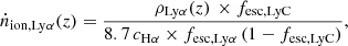 (6)
(6)
where cHα is the coefficient factor of the Hα emission line, ∼1.25 − 1.35 × 10⁻¹² for Case B recombination. It remains to estimate the individual parameters appearing in the above function.
– The LAE luminosity density (ρLyα): this parameter was presented in Sect. 3.3.
– The escape fraction of Lyman-α photons, fesc, Lyα. We cannot correct ρLyα by the escape fraction derived in Sect. 3.3 as this, by construction, corrects ρLyα to the total value of the parent population (ρtotal) that we take from Bouwens et al. (2022). We can nonetheless use the value we have derived in Sect. 2. We discuss both our sample median, fesc, Lyα = 22.5% and the sample median for the LAEs at z > 5, fesc, Lyα = 36%.
– LyC escape fraction, fesc, LyC: This parameter is poorly understood, in particular at high redshift, due to the increasing IGM neutrality, which absorbs Lyman continuum photons along the light of sight. However, recent progress has been made in local galaxies (high-redshift analogues) (Flury et al. 2022; Izotov et al. 2024) and in LAEs up to z ∼ 3 (Liu et al. 2023; Kerutt et al. 2024; Pahl et al. 2024; Jung et al. 2024a). However, results from these studies, as well as simulations (Choustikov et al. 2024a), suggest that there is a significant scatter in the fesc, LyC across the LAE population. Therefore, placing one value on fesc, LyC, such as fesc, Lyα, is a simplification. Many observational studies point to values between 10% and 15%: Kerutt et al. (2024) derive an underlying population value of 12%, Jung et al. (2024a) obtain values between 3% and 15%, Liu et al. (2023) give an upper limit of 16% and Izotov et al. (2024) find values between 1% and 34%, with most of their galaxies having fesc,LyC < 15%. Based on the SPHINX simulations (Garel et al. 2021) and the model for Lyman continuum escape developed by Rosdahl et al. (2022), fesc, LyC is 1.17%,0.4% at MUV = −17, −13 (we note that this is for all galaxies, not just those selected as LAEs).
The ability to turn Eq. (6) into a summation, with each LAE contributing its own ρLyα, fesc, Lyα and with fesc, LyC consequently following a relation such as those presented in Rosdahl et al. (2022), Choustikov et al. (2024a) or Izotov et al. (2024) would be an improvement. Increased statistics, especially for faint LAEs and at redshifts greater than 5 would be necessary to make this approach feasible. This is within reach for JWST in the coming years, as observed samples increase in size and more faint galaxies are uncovered.
A very recent approach by Choustikov et al. (2024b) attempts this individual approach for a large sample of JWST/NIRCam-observed galaxies (not just LAEs) (observed by the JADES programme, Eisenstein et al. 2023). The authors conclude that faint galaxies (MUV ≥ −18.5) are potentially responsible for ∼80% of the reionisation budget. The majority of our sample of LAEs fall within this bracket (see, e.g. Fig. 6).
With  , at z = 6, from Eq. (6), we can compare this value to the ionising emissivity required for reionisation as derived by Bouwens et al. (2015a),
  (we note that this value uses a fiducial clumping factor CHII = 3). In Table 2, we show the range of results, applying different values for ρLyα, fesc, Lyα and fesc, LyC. For ρLyα derived from our results, (the LF of Thai et al. 2023) we find LAE contributions ranging from minor (5–10%) for a low fesc, LyC (0.4%) to dominant > 100% for fesc, LyC = 10%. Changing fesc, Lyα between the sample median and z > 5 median does not qualitatively change the outcome. As fesc, LyC changes more significantly depending on the chosen value, this represents the main effect on the outcome. In several cases we see unrealistic contributions (> 100%) for LAEs based on fesc, LyC = 10%, suggesting that this value may be too high and not representative of our whole sample. Crucial work remains to correlate fesc, LyC with observable parameters (such as Lyman-α parameters) at higher redshifts and constrain the escape of ionising photons for the LAE population at z ∼ 6 and above.
LAE contribution to reionisation.
We investigate the effect on the LAE reionisation contribution in the case of a completeness cut in the calculation of the LAE LF at 10%. We take the results of de La Vieuville et al. (2019) as emblematic of this scenario (as mentioned, the LF of Thai et al. (2023) is consistent with that of de La Vieuville et al. (2019) if this cut is applied). In this case, the contribution to reionisation derived for the LAE population is significantly less (1 − 2% for fesc, LyC = 0.4% and 30 − 50% for fesc, LyC = 10%). This emphasises the sensitivity of these results to the completeness treatment applied for the LAE population.
We additionally show the difference between the modified Schechter function, which we have chosen to adopt throughout this study, and the general Schechter function (noted GSF in Table 2. Using the general Schechter function roughly doubles the LAE contribution to reionisation.
Highlighting the effects of both the function chosen to fit the LAE LF and the completeness cut applied serves to reinforce the need for a larger sample at z > 5 and for faint galaxies. Better statistics in this parameter space will constrain the faint end of the LF more strongly, discriminating between the modified and general Schechter functions. With deeper observations of faint galaxies, the completeness for the faint LAEs will also improve (i.e. the sample will be more complete at a given Lyman-α luminosity) and the chosen cut will become a less important factor.
The chosen value of fesc, LyC is clearly determinant in this calculation with LAEs contributing very little for small values of fesc, LyC and providing the dominant contribution for reasonable values of fesc, LyC observed in many lower-redshift LAEs and low-mass galaxies acting as high-redshift analogs. Using the ρLyα from Thai et al. (2023) and fesc, Lyα = 36%, a sample average fesc, LyC of just 6.5% would be enough for LAEs to provide all the necessary ionising photons at z = 6. If the values of fesc, LyC observed in these low-redshift LAEs are maintained across the LAE population into reionisation, it is certainly conceivable that these galaxies could have been responsible for reionisation in its entirety. We note that the results in this study do not constrain the reionisation scenario beyond z = 6.7 and that LAE LFs at z ≥ 7 are needed to track the contribution of LAEs further into the EoR.
5. Conclusions
We have derived the escape fraction of Lyman-α photons across the redshift range 2.9 < z < 6.7 using two methods, namely, comparing dust-corrected star formation to star formation derived from Lyman-α emission and comparing the SFRD from the UV ‘parent’ population LF and the Lyman-α SFRD derived from the LAE LF. Here we summarise the main conclusions of the work.
– We determined the values of fesc, Lyα for 96 individual galaxies behind the A2744 lensing cluster, finding a significant scatter and a sample median of 22.5%.
– We observed a significant evolution of fesc, Lyα with absolute UV magnitude, following the relation log(fesc, Lyα) = (0.28 ± 0.03) MUV + (4.3 ± 0.6). Notably, we saw very few LAEs with fesc, Lyα < 10% among objects fainter than MUV = −18.
– We expect the line-incompleteness of MUSE Lyman-α detections to play a role here, but only for the faintest objects, MUV ≳ −14.
– For the global redshift evolution of fesc, Lyα, we derived results in agreement with previous determinations in the literature when using a bright LF integration limit (0.04L*). fesc, Lyα appears to reach 100% around z = 11 − 12.
– When we assessed fesc, Lyα with an integration limit that reflects the faint limits of our sample (0.0006L*), we found that fesc, Lyα becomes consistent with 100% escape by z ∼ 6. This result supports galaxies being chemically unevolved and highly star forming at these redshifts, producing a high quantity of Lyman-α photons and allowing them to escape.
– With both bright and faint integration limits, we observed little evolution between z = 3 − 5 and a jump at z ∼ 6, suggesting a rapid evolution of the LAE population towards reionisation, although this effect is at < 1σ for our dataset.
– We saw more significant redshift evolution in our global assessment than for individual galaxies due to the large intrinsic scatter in the LAE population combined with the far greater statistics in the respective LFs used for the global comparison.
– We revisited the LAE contribution to the reionisation process, taking into account our new values for fesc, Lyα and a range of motivated values for fesc, LyC. The results depend heavily on the assumed values for fesc, LyC. Taking the latest values observed in LAEs at z ∼ 3, we find that LAEs can provide all the ionising emissivity needed for reionisation.
– We demonstrated the additional strong dependence of the LAE contribution on the completeness cuts and fitting form of the LAE LF. This stresses the urgent need for better statistics at z > 5 and log LLyα[erg/s]< 40.
At the moment, it is challenging to improve the two luminosity functions used in this work, as they already use the full extent of deep observations in lensing clusters from HFF and MUSE. Further clusters to be included in this sample are desirable, particularly to better constrain the high-redshift (z ∼ 6) faint end of the LAE LF. This will be made possible through further MUSE-observed lensing clusters, such as those presented in Claeyssens et al. (in prep.). This will also help bin the results into smaller redshift bins to better constrain the precise evolution in the range 3 < z < 6. Observations of LAEs at higher redshift from JWST, such as Chen et al. (2024), Tang et al. (2024), Lin et al. (2024), Witstok et al. (2024a), Nakane et al. (2024) are starting to build larger sample sizes, but they are not yet at the quantity of LAEs and UV-selected galaxies used for the results in this work. In particular, intrinsically faint galaxies have poor statistics, although this can be improved with the continuing observations of lensing clusters by JWST/NIRCam and JWST/NIRSpec.
On the other hand, it is possible, with further JWST observations, photometry, and spectroscopy in order to improve the fesc, Lyα determinations for individual galaxies. The Balmer decrement provides accurate estimations of dust attenuation along with SED fitting utilising a greater number of photometric bands and a more extended coverage. Studying these systems in more detail will reveal the range of different escape scenarios leading to the varied fesc, Lyα values that we have observed. This can, in turn, lead to better understanding of galaxy evolution around the epoch of reionisation and how LAEs affect this process.
Acknowledgments
This work is done based on observations made with ESO Telescopes at the La Silla Paranal Observatory under programme IDs 060.A-9345, 092.A-0472, 094.A-0115, 095.A-0181, 096.A-0710, 097.A0269, 100.A-0249, and 294.A-5032. Also based on observations obtained with the NASA/ESA Hubble Space Telescope, retrieved from the Mikulski Archive for Space Telescopes (MAST) at the Space Telescope Science Institute (STScI). STScI is operated by the Association of Universities for Research in Astronomy, Inc. under NASA contract NAS 5-26555. All plots in this paper were created using Matplotlib (Hunter 2007). Part of this work was supported by the French CNRS, the Aix-Marseille University, the French Programme National de Cosmologie et Galaxies (PNCG) of CNRS/INSU with INP and IN2P3, co-funded by CEA and CNES. This work also received support from the French government under the France 2030 investment plan, as part of the Excellence Initiative of Aix-Marseille University - A*MIDEX (AMX-19-IET-008 - IPhU). Financial support from the World Laboratory, the Odon Vallet Foundation and VNSC is gratefully acknowledged. Tran Thi Thai was funded by Vingroup JSC and supported by the Master, PhD Scholarship Programme of Vingroup Innovation Foundation (VINIF), Institute of Big Data, code VINIF.2023.TS.108. This research was funded by Vingroup Innovation Foundation under project code VINIF.2023.DA.057.
References
- Acebron, A., Jullo, E., Limousin, M., et al. 2017, MNRAS, 470, 1809 [Google Scholar]
- Arrabal Haro, P., Rodríguez Espinosa, J., Muñoz-Tuñón, C., et al. 2018, MNRAS, 478, 3740 [NASA ADS] [CrossRef] [Google Scholar]
- Atek, H., Kunth, D., Hayes, M., Östlin, G., & Mas-Hesse, J. M. 2008, A&A, 488, 491 [NASA ADS] [CrossRef] [EDP Sciences] [Google Scholar]
- Atek, H., Labbé, I., Furtak, L. J., et al. 2024, Nature, 626, 975 [NASA ADS] [CrossRef] [Google Scholar]
- Austin, D., Conselice, C. J., Adams, N. J., et al. 2024, ArXiv e-prints [arXiv:2404.10751] [Google Scholar]
- Bacon, R., Brinchmann, J., Richard, J., et al. 2015, A&A, 575, A75 [NASA ADS] [CrossRef] [EDP Sciences] [Google Scholar]
- Bacon, R., Brinchmann, J., Conseil, S., et al. 2023, A&A, 670, A4 [NASA ADS] [CrossRef] [EDP Sciences] [Google Scholar]
- Beauchesne, B., Clément, B., Hibon, P., et al. 2023, MNRAS, 527, 3246 [CrossRef] [Google Scholar]
- Bertin, E., & Arnouts, S. 1996, A&AS, 117, 393 [NASA ADS] [CrossRef] [EDP Sciences] [Google Scholar]
- Bezanson, R., Labbe, I., Whitaker, K. E., et al. 2022, ArXiv e-prints [arXiv:2212.04026] [Google Scholar]
- Blaizot, J., Garel, T., Verhamme, A., et al. 2023, MNRAS, 523, 3749 [NASA ADS] [CrossRef] [Google Scholar]
- Blanc, G. A., Adams, J. J., Gebhardt, K., et al. 2011, ApJ, 736, 31 [CrossRef] [Google Scholar]
- Boquien, M., Burgarella, D., Roehlly, Y., et al. 2019, A&A, 622, A103 [NASA ADS] [CrossRef] [EDP Sciences] [Google Scholar]
- Bouwens, R. J., Illingworth, G. D., Franx, M., et al. 2009, ApJ, 705, 936 [Google Scholar]
- Bouwens, R. J., Illingworth, G. D., Oesch, P. A., et al. 2010, ApJ, 709, L133 [CrossRef] [Google Scholar]
- Bouwens, R. J., Illingworth, G., Oesch, P., et al. 2015a, ApJ, 803, 34 [CrossRef] [Google Scholar]
- Bouwens, R. J., Illingworth, G. D., Oesch, P. A., et al. 2015b, ApJ, 811, 140 [NASA ADS] [CrossRef] [Google Scholar]
- Bouwens, R. J., Aravena, M., Decarli, R., et al. 2016, ApJ, 833, 72 [NASA ADS] [CrossRef] [Google Scholar]
- Bouwens, R. J., Illingworth, G., Ellis, R. S., Oesch, P., & Stefanon, M. 2022, ApJ, 940, 55 [NASA ADS] [CrossRef] [Google Scholar]
- Brocklehurst, M. 1971, MNRAS, 153, 471 [Google Scholar]
- Bruzual, G., & Charlot, S. 2003, MNRAS, 344, 1000 [NASA ADS] [CrossRef] [Google Scholar]
- Buat, V., Noll, S., Burgarella, D., et al. 2012, A&A, 545, A141 [NASA ADS] [CrossRef] [EDP Sciences] [Google Scholar]
- Calzetti, D., Armus, L., Bohlin, R. C., et al. 2000, ApJ, 533, 682 [NASA ADS] [CrossRef] [Google Scholar]
- Caruana, J., Wisotzki, L., Herenz, E. C., et al. 2018, MNRAS, 473, 30 [NASA ADS] [CrossRef] [Google Scholar]
- Cassata, P., Le Fèvre, O., Garilli, B., et al. 2011, A&A, 525, A143 [NASA ADS] [CrossRef] [EDP Sciences] [Google Scholar]
- Chabrier, G. 2003, PASP, 115, 763 [Google Scholar]
- Chen, Z., Stark, D. P., Mason, C., et al. 2024, MNRAS, 528, 7052 [CrossRef] [Google Scholar]
- Choustikov, N., Katz, H., Saxena, A., et al. 2024a, MNRAS, [arXiv:2401.09557] [Google Scholar]
- Choustikov, N., Stiskalek, R., Saxena, A., et al. 2024b, ArXiv e-prints [arXiv:2405.09720] [Google Scholar]
- Ciardullo, R., Zeimann, G. R., Gronwall, C., et al. 2014, ApJ, 796, 64 [CrossRef] [Google Scholar]
- Claeyssens, A., Richard, J., Blaizot, J., et al. 2022, A&A, 666, A78 [NASA ADS] [CrossRef] [EDP Sciences] [Google Scholar]
- Covone, G., Kneib, J. P., Soucail, G., et al. 2006, A&A, 456, 409 [NASA ADS] [CrossRef] [EDP Sciences] [Google Scholar]
- Cowie, L. L., & Hu, E. M. 1998, AJ, 115, 1319 [Google Scholar]
- De Barros, S., Pentericci, L., Vanzella, E., et al. 2017, A&A, 608, A123 [NASA ADS] [CrossRef] [EDP Sciences] [Google Scholar]
- de La Vieuville, G., Bina, D., Pello, R., et al. 2019, A&A, 628, A3 [NASA ADS] [CrossRef] [EDP Sciences] [Google Scholar]
- de La Vieuville, G., Pelló, R., Richard, J., et al. 2020, A&A, 644, A39 [NASA ADS] [CrossRef] [EDP Sciences] [Google Scholar]
- Dijkstra, M. 2016, Understanding the Epoch of Cosmic Reionization: Challenges and Progress (Springer), 145 [NASA ADS] [CrossRef] [Google Scholar]
- Dijkstra, M., & Kramer, R. 2012, MNRAS, 424, 1672 [NASA ADS] [CrossRef] [Google Scholar]
- Dijkstra, M., Gronke, M., & Venkatesan, A. 2016, ApJ, 828, 71 [Google Scholar]
- Drake, A.-B., Garel, T., Wisotzki, L., et al. 2017, A&A, 608, A6 [NASA ADS] [CrossRef] [EDP Sciences] [Google Scholar]
- Duncan, K., & Conselice, C. J. 2015, MNRAS, 451, 2030 [NASA ADS] [CrossRef] [Google Scholar]
- Eisenstein, D. J., Willott, C., Alberts, S., et al. 2023, ArXiv e-prints [arXiv:2306.02465] [Google Scholar]
- Ferrara, A. 2024, A&A, 684, A207 [NASA ADS] [CrossRef] [EDP Sciences] [Google Scholar]
- Finkelstein, S. L. 2016, PASA, 33, e037 [Google Scholar]
- Finkelstein, S. L., Malhotra, S., Rhoads, J. E., Hathi, N. P., & Pirzkal, N. 2009, MNRAS, 393, 1174 [NASA ADS] [CrossRef] [Google Scholar]
- Flury, S. R., Jaskot, A. E., Ferguson, H. C., et al. 2022, ApJS, 260, 1 [NASA ADS] [CrossRef] [Google Scholar]
- Furtak, L. J., Atek, H., Lehnert, M. D., Chevallard, J., & Charlot, S. 2021, MNRAS, 501, 1568 [Google Scholar]
- Garel, T., Blaizot, J., Rosdahl, J., et al. 2021, MNRAS, 504, 1902 [NASA ADS] [CrossRef] [Google Scholar]
- Gazagnes, S., Cullen, F., Mauerhofer, V., et al. 2024, ApJ, 969, 50 [NASA ADS] [CrossRef] [Google Scholar]
- Giovinazzo, E., Trebitsch, M., Mauerhofer, V., Dayal, P., & Oesch, P. A. 2024, A&A, 688, A122 [NASA ADS] [CrossRef] [EDP Sciences] [Google Scholar]
- Gnedin, N. Y. 2016, ApJ, 825, L17 [Google Scholar]
- Goovaerts, I., Pello, R., Thai, T. T., et al. 2023, A&A, 678, A174 [NASA ADS] [CrossRef] [EDP Sciences] [Google Scholar]
- Goovaerts, I., Pello, R., Burgarella, D., et al. 2024, A&A, 683, A184 [NASA ADS] [CrossRef] [EDP Sciences] [Google Scholar]
- Gronke, M., & Dijkstra, M. 2016, ApJ, 826, 14 [NASA ADS] [CrossRef] [Google Scholar]
- Hansen, M., & Oh, S. P. 2006, MNRAS, 367, 979 [NASA ADS] [CrossRef] [Google Scholar]
- Hashimoto, T., Verhamme, A., Ouchi, M., et al. 2015, ApJ, 812, 157 [Google Scholar]
- Hayes, M., Östlin, G., Schaerer, D., et al. 2010, Nature, 464, 562 [NASA ADS] [CrossRef] [Google Scholar]
- Hayes, M., Schaerer, D., Östlin, G., et al. 2011, ApJ, 730, 8 [NASA ADS] [CrossRef] [Google Scholar]
- Hayes, M., Östlin, G., Schaerer, D., et al. 2013, ApJ, 765, L27 [NASA ADS] [CrossRef] [Google Scholar]
- Hu, E. M., Cowie, L. L., & McMahon, R. G. 1998, ApJ, 502, L99 [NASA ADS] [CrossRef] [Google Scholar]
- Iani, E., Caputi, K. I., Rinaldi, P., et al. 2023, ArXiv e-prints [arXiv:2309.08515] [Google Scholar]
- Izotov, Y. I., Chisholm, J., Worseck, G., et al. 2022, MNRAS, 515, 2864 [NASA ADS] [CrossRef] [Google Scholar]
- Izotov, Y. I., Thuan, T. X., Guseva, N. G., et al. 2024, MNRAS, 527, 281 [Google Scholar]
- Jaacks, J., Thompson, R., & Nagamine, K. 2013, ApJ, 766, 94 [NASA ADS] [CrossRef] [Google Scholar]
- Jiang, H., Wang, X., Cheng, C., et al. 2023, ArXiv e-prints [arXiv:2312.04151] [Google Scholar]
- Jung, I., Ferguson, H. C., Hayes, M. J., et al. 2024a, ArXiv e-prints [arxiv:2403.02388v1] [Google Scholar]
- Jung, I., Finkelstein, S. L., Arrabal Haro, P., et al. 2024b, ApJ, 967, 73 [NASA ADS] [CrossRef] [Google Scholar]
- Kennicutt, R. C. 1998a, ApJ, 498, 541 [NASA ADS] [CrossRef] [Google Scholar]
- Kennicutt, R. C. 1998b, ARA&A, 36, 189 [NASA ADS] [CrossRef] [Google Scholar]
- Kerutt, J., Oesch, P. A., Wisotzki, L., et al. 2024, A&A, 684, A42 [NASA ADS] [CrossRef] [EDP Sciences] [Google Scholar]
- Konno, A., Ouchi, M., Nakajima, K., et al. 2016, ApJ, 823, 20 [Google Scholar]
- Kusakabe, H., Blaizot, J., Garel, T., et al. 2020, A&A, 638, A12 [NASA ADS] [CrossRef] [EDP Sciences] [Google Scholar]
- Lagattuta, D. J., Richard, J., Bauer, F. E., et al. 2019, MNRAS, 485, 3738 [NASA ADS] [Google Scholar]
- Lam, Bouwens., Rychard, J., Labbé, Ivo., et al. 2019, A&A, 627, A164 [NASA ADS] [CrossRef] [EDP Sciences] [Google Scholar]
- Limousin, M., Richard, J., Jullo, E., et al. 2016, A&A, 588, A99 [NASA ADS] [CrossRef] [EDP Sciences] [Google Scholar]
- Lin, X., Cai, Z., Wu, Y., et al. 2024, ApJS, 272, 33 [NASA ADS] [CrossRef] [Google Scholar]
- Liu, Y., Jiang, L., Windhorst, R. A., Guo, Y., & Zheng, Z.-Y. 2023, ApJ, 958, 22 [NASA ADS] [CrossRef] [Google Scholar]
- Lotz, J. E., Koekemoer, A., Coe, D., et al. 2017, ApJ, 837, 97 [NASA ADS] [CrossRef] [Google Scholar]
- Madau, P., & Dickinson, M. 2014, ARA&A, 52, 415 [Google Scholar]
- Madau, P., Haardt, F., & Rees, M. J. 1999, ApJ, 514, 648 [CrossRef] [Google Scholar]
- Mahler, G., Richard, J., Clément, B., et al. 2018, MNRAS, 473, 663 [Google Scholar]
- Małek, K., Buat, V., Roehlly, Y., et al. 2018, A&A, 620, A50 [Google Scholar]
- Maseda, M. V., Bacon, R., Franx, M., et al. 2018, ApJ, 865, L1 [Google Scholar]
- Maseda, M. V., Bacon, R., Lam, D., et al. 2020, MNRAS, 493, 5120 [Google Scholar]
- Maseda, M. V., Lewis, Z., Matthee, J., et al. 2023, ApJ, 956, 11 [NASA ADS] [CrossRef] [Google Scholar]
- Matthee, J., Sobral, D., Best, P., et al. 2016a, MNRAS, 465, 3637 [Google Scholar]
- Matthee, J., Sobral, D., Oteo, I., et al. 2016b, MNRAS, 458, 449 [Google Scholar]
- Matthee, J., Sobral, D., Hayes, M., et al. 2021, MNRAS, 505, 1382 [NASA ADS] [CrossRef] [Google Scholar]
- Matthee, J., Naidu, R. P., Pezzulli, G., et al. 2022, MNRAS, 512, 5960 [NASA ADS] [CrossRef] [Google Scholar]
- McClymont, W., Tacchella, S., D’Eugenio, F., et al. 2024, ArXiv e-prints [arXiv:2405.15859] [Google Scholar]
- McGreer, I. D., Fan, X., Jiang, L., & Cai, Z. 2018, AJ, 155, 131 [NASA ADS] [CrossRef] [Google Scholar]
- Naidu, R. P., Oesch, P. A., van Dokkum, P., et al. 2022, ApJ, 940, L14 [NASA ADS] [CrossRef] [Google Scholar]
- Nakane, M., Ouchi, M., Nakajima, K., et al. 2024, ApJ, 967, 28 [NASA ADS] [CrossRef] [Google Scholar]
- Nanayakkara, T., Glazebrook, K., Jacobs, C., et al. 2023, ApJ, 947, L26 [NASA ADS] [CrossRef] [Google Scholar]
- Napolitano, L., Pentericci, L., Santini, P., et al. 2024, A&A, 688, A106 [NASA ADS] [CrossRef] [EDP Sciences] [Google Scholar]
- Oesch, P. A., Bouwens, R. J., Illingworth, G. D., Labbé, I., & Stefanon, M. 2018, ApJ, 855, 105 [Google Scholar]
- Osterbrock, D. E. 1989, Astrophysics of Gaseous Nebulae and Active Galactic Nuclei (University Science Books) [Google Scholar]
- Osterbrock, D. E., & Ferland, G. J. 2006, Astrophysics Of Gas Nebulae and Active Galactic Nuclei (University science books) [Google Scholar]
- Ouchi, M., Shimasaku, K., Okamura, S., et al. 2004, ApJ, 611, 660 [Google Scholar]
- Ouchi, M., Shimasaku, K., Akiyama, M., et al. 2008, ApJS, 176, 301 [Google Scholar]
- Oyarzún, G. A., Blanc, G. A., González, V., Mateo, M., & Bailey, J. I. 2017, ApJ, 843, 133 [CrossRef] [Google Scholar]
- Pahl, A. J., Shapley, A. E., Steidel, C. C., et al. 2024, Arxiv e-prints [arxiv:2401.09526v1] [Google Scholar]
- Parsa, S., Dunlop, J. S., McLure, R. J., & Mortlock, A. 2016, MNRAS, 456, 3194 [Google Scholar]
- Pello, R., Le Borgne, J.-F., Soucail, G., Mellier, Y., & Sanahuja, B. 1991, ApJ, 366, 405 [NASA ADS] [CrossRef] [Google Scholar]
- Pentericci, L., Fontana, A., Vanzella, E., et al. 2011, ApJ, 743, 132 [NASA ADS] [CrossRef] [Google Scholar]
- Pentericci, L., Vanzella, E., Castellano, M., et al. 2018, A&A, 619, A147 [NASA ADS] [CrossRef] [EDP Sciences] [Google Scholar]
- Piqueras, L., Conseil, S., Shepherd, M., et al. 2019, ASP Conf. Ser., 521, 545 [Google Scholar]
- Planck Collaboration VI. 2020, A&A, 641, A6 [NASA ADS] [CrossRef] [EDP Sciences] [Google Scholar]
- Postman, M., Coe, D., Benítez, N., et al. 2012, ApJS, 199, 25 [Google Scholar]
- Reddy, N. A., Steidel, C. C., Pettini, M., et al. 2008, ApJS, 175, 48 [CrossRef] [Google Scholar]
- Reddy, N. A., Oesch, P. A., Bouwens, R. J., et al. 2018, ApJ, 853, 56 [NASA ADS] [CrossRef] [Google Scholar]
- Richard, J., Smith, G. P., Kneib, J.-P., et al. 2010, MNRAS, 404, 325 [NASA ADS] [Google Scholar]
- Richard, J., Claeyssens, A., Lagattuta, D., et al. 2021, A&A, 646, A83 [EDP Sciences] [Google Scholar]
- Robertson, B. E., Furlanetto, S. R., Schneider, E., et al. 2013, ApJ, 768, 71 [Google Scholar]
- Rosdahl, J., Blaizot, J., Katz, H., et al. 2022, MNRAS, 515, 2386 [CrossRef] [Google Scholar]
- Runnholm, A., Hayes, M., Melinder, J., et al. 2020, ApJ, 892, 48 [NASA ADS] [CrossRef] [Google Scholar]
- Salpeter, E. E. 1955, ApJ, 121, 161 [Google Scholar]
- Saxena, A., Bunker, A. J., Jones, G. C., et al. 2024, A&A, 684, A84 [NASA ADS] [CrossRef] [EDP Sciences] [Google Scholar]
- Schaerer, D., & Verhamme, A. 2008, A&A, 480, 369 [NASA ADS] [CrossRef] [EDP Sciences] [Google Scholar]
- Schaerer, D., de Barros, S., & Stark, D. P. 2011, A&A, 536, A72 [NASA ADS] [CrossRef] [EDP Sciences] [Google Scholar]
- Shipley, H. V., Lange-Vagle, D., Marchesini, D., et al. 2018, ApJS, 235, 14 [Google Scholar]
- Simmonds, C., Tacchella, S., Maseda, M., et al. 2023, MNRAS, 523, 5468 [NASA ADS] [CrossRef] [Google Scholar]
- Sobral, D., & Matthee, J. 2019, A&A, 623, A157 [NASA ADS] [CrossRef] [EDP Sciences] [Google Scholar]
- Sobral, D., Matthee, J., Best, P., et al. 2017, MNRAS, 466, 1242 [Google Scholar]
- Sobral, D., Santos, S., Matthee, J., et al. 2018, MNRAS, 476, 4725 [Google Scholar]
- Song, M., Finkelstein, S. L., Gebhardt, K., et al. 2014, ApJ, 791, 3 [Google Scholar]
- Stark, D. P., Ellis, R. S., Chiu, K., Ouchi, M., & Bunker, A. 2010, MNRAS, 408, 1628 [Google Scholar]
- Stark, D. P., Ellis, R. S., & Ouchi, M. 2011, ApJ, 728, L2 [Google Scholar]
- Steidel, C. C., Bogosavljević, M., Shapley, A. E., et al. 2018, ApJ, 869, 123 [Google Scholar]
- Tang, M., Stark, D. P., Ellis, R. S., et al. 2024, MNRAS, 531, 2701 [NASA ADS] [CrossRef] [Google Scholar]
- Thai, T., Tuan-Anh, P., Pello, R., et al. 2023, A&A, 678, A139 [NASA ADS] [CrossRef] [EDP Sciences] [Google Scholar]
- Theulé, P., Burgarella, D., Buat, V., et al. 2024, A&A, 682, A119 [NASA ADS] [CrossRef] [EDP Sciences] [Google Scholar]
- Topping, M. W., Stark, D. P., Endsley, R., et al. 2022, ApJ, 941, 153 [NASA ADS] [CrossRef] [Google Scholar]
- Trainor, R. F., Strom, A. L., Steidel, C. C., & Rudie, G. C. 2016, ApJ, 832, 171 [NASA ADS] [CrossRef] [Google Scholar]
- Treu, T., Schmidt, K., Brammer, G., et al. 2015, ApJ, 812, 114 [NASA ADS] [CrossRef] [Google Scholar]
- Verhamme, A., Schaerer, D., Atek, H., & Tapken, C. 2008, A&A, 491, 89 [NASA ADS] [CrossRef] [EDP Sciences] [Google Scholar]
- Verhamme, Dubois Y., Blaizot, J., et al. 2012, A&A, 546, A111 [NASA ADS] [CrossRef] [EDP Sciences] [Google Scholar]
- Verhamme, A., Orlitová, I., Schaerer, D., et al. 2017, A&A, 597, A13 [NASA ADS] [CrossRef] [EDP Sciences] [Google Scholar]
- Vitte, E., Verhamme, A., Hibon, P., et al. 2024, A&A, submitted [Google Scholar]
- Weaver, J. R., Cutler, S. E., Pan, R., et al. 2023, ArXiv e-prints [arXiv:2301.02671] [Google Scholar]
- Weilbacher, P. M., Palsa, R., Streicher, O., et al. 2020, A&A, 641, A28 [NASA ADS] [CrossRef] [EDP Sciences] [Google Scholar]
- Wilkins, S. M., Bunker, A., Coulton, W., et al. 2013, MNRAS, 430, 2885 [NASA ADS] [CrossRef] [Google Scholar]
- Witstok, J., Maiolino, R., Smit, R., et al. 2024a, ArXiv e-prints [arXiv:2404.05724] [Google Scholar]
- Witstok, J., Smit, R., Saxena, A., et al. 2024b, A&A, 682, A40 [NASA ADS] [CrossRef] [EDP Sciences] [Google Scholar]
- Witten, C., Laporte, N., Martin-Alvarez, S., et al. 2024, Nat. Astron., 8, 384 [Google Scholar]
- Yang, H., Malhotra, S., Gronke, M., et al. 2017, ApJ, 844, 171 [NASA ADS] [CrossRef] [Google Scholar]
- Yuan, Y., Martin-Alvarez, S., Haehnelt, M. G., Garel, T., & Sijacki, D. 2024, MNRAS, 532, 3643 [NASA ADS] [CrossRef] [Google Scholar]
- Yue, B., Ferrara, A., & Xu, Y. 2016, MNRAS, 463, 1968 [NASA ADS] [CrossRef] [Google Scholar]
- Zheng, Z., Cen, R., Trac, H., & Miralda-Escudé, J. 2010, ApJ, 716, 574 [NASA ADS] [CrossRef] [Google Scholar]
- Zheng, Z.-Y., Finkelstein, S. L., Finkelstein, K., et al. 2013, MNRAS, 431, 3589 [Google Scholar]
Appendix A: LAE luminosity density and its star-forming rate density
LAE luminosity density and its SFRD.
All Tables
All Figures
|
Fig. 1. Redshift evolution of the escape fraction of Lyman-α photons from LAEs in the A2744 lensing cluster colour-coded by the absolute UV magnitude of each LAE. The global medians of our sample and that in B11, are shown with red and cyan dashed lines respectively. The median uncertainty of the sample (∼18%) is shown by the black error bar, as if it was at the level of the global median, offset for clarity. |
| In the text | |
|
Fig. 2. Evolution of fesc, Lyα with absolute UV magnitude MUV. Photometrically detected galaxies are split into three redshift bins to stress the lack of evolution in this sense, while the evolution with MUV is fit by the relation in cyan (details in text). Median error bars for the three redshift bins are shown in the corresponding colour and fesc, Lyα error bars are also listed here for clarity (relevant redshift bin in brackets): 0.18 (2.9 < z < 4), 0.12 (4 < z < 5) and 0.25 (5 < z < 6.7). Absolute magnitude values and their errors are adjusted for magnification. Black triangles denote continuum-undetected LAEs. MUV values are upper limits and escape fraction values are lower limits. These objects are not included in the fit. Red shaded areas denote regions of incompleteness based on MUSE line-detections: a darker colour representing increasing lensing magnification (see text). |
| In the text | |
|
Fig. 3. Ultraviolet and LAE LFs included in our analysis on a common x-axis of SFR. The LFs of Bouwens et al. (2022) and Thai et al. (2023) are shown in bold and the literature LFs are shown in coloured dash-dotted lines. The LF integration limits in terms of L* that we use throughout this work are denoted by the pink shaded regions. Left: Results from the redshift range 3 to 4. Right: Results from the redshift range 5 to 6. The literature LFs in the graph are shown in shorthand in the caption and here in full, in order: Ouchi et al. (2008), Cassata et al. (2011), Sobral et al. (2018), Thai et al. (2023), Drake et al. (2017), Bouwens et al. (2022, 2009). |
| In the text | |
|
Fig. 4. Global redshift evolution of fesc, Lyα with an integration limit on both LFs of 0.04L*. Our results, using the LFs from Thai et al. (2023) are shown in cyan for the modified Schechter function and pink for the general Schechter function. The dotted horizontal line denotes fesc = 100%. The dash-dotted green curve is from Hayes et al. (2011) in the redshift range of 2.2 − 6.6 and calculated with the integration limit 0.04L*. The red dash-dotted curve is the best fit to all the data shown and the blue dash-dotted curve fits just the data of Thai et al. (2023) (cyan points: modified Schechter function). |
| In the text | |
|
Fig. 5. Global redshift evolution of fesc, Lyα with an integration limit on both LFs of 0.0006L*. Results from this study are shown by cyan (modified Schechter function) and pink (general Schechter function) points. Power-law fits from the literature are shown in grey and green (B11, Hayes et al. 2011) and the equivalent fit to all the data is shown in red. The fit from Hayes et al. (2011) is derived from results integrated to 0.04L*, and the fit from B11 from results integrated to 0. |
| In the text | |
|
Fig. 6. Redshift and MUV distribution of LAEs and Lyman-break galaxies (UV-selected galaxies) from the sample in Goovaerts et al. (2023). Grey points denote the Lyman-break galaxies and are thus analogous to the UV-selected sample. Orange points denote objects that were selected as LBGs and LAEs and upwards-facing triangles indicate LAEs that were not detected at all in the HST imaging (Shipley et al. 2018). The 2σ upper limits for the continuum of these objects have been estimated using the local noise in the region where they would have been detected in the HST image that would see the 1500 Å emission. The horizontal dashed line denotes the integration limit in the ρtotal calculation in Bouwens et al. (2022). |
| In the text | |
Current usage metrics show cumulative count of Article Views (full-text article views including HTML views, PDF and ePub downloads, according to the available data) and Abstracts Views on Vision4Press platform.
Data correspond to usage on the plateform after 2015. The current usage metrics is available 48-96 hours after online publication and is updated daily on week days.
Initial download of the metrics may take a while.