| Issue |
A&A
Volume 690, October 2024
|
|
|---|---|---|
| Article Number | A149 | |
| Number of page(s) | 9 | |
| Section | Extragalactic astronomy | |
| DOI | https://doi.org/10.1051/0004-6361/202450757 | |
| Published online | 04 October 2024 | |
Simulations of cluster ultra-diffuse galaxies in MOND
1
Université de Strasbourg, CNRS, Observatoire Astronomique de Strasbourg, UMR 7550, F-67000 Strasbourg, France
2
LERMA, Observatoire de Paris, CNRS, PSL Univ., Sorbonne Univ., 75014 Paris, France
3
Instituto de Física y Astronomía, Universidad de Valparaíso, Gran Bretaña 1111, Valparaíso, Chile
4
Institute of Physics, Laboratory of Astrophysics, Ecole Polytechnique Fédérale de Lausanne (EPFL), 1290 Sauverny, Switzerland
5
Scottish Universities Physics Alliance, University of Saint Andrews, North Haugh, Saint Andrews, Fife KY16 9SS, UK
Received:
17
May
2024
Accepted:
2
July
2024
Abstract
Ultra-diffuse galaxies (UDGs) in the Coma cluster have velocity dispersion profiles that are in full agreement with the predictions of modified Newtonian dynamics (MOND) in isolation. However, the external field effect (EFE) from the cluster seriously undermines this agreement. It has been suggested that this could be related to the fact that UDGs are out-of-equilibrium objects whose stars have been heated by the cluster tides or that they recently fell onto the cluster on radial orbits; thus, their velocity dispersion may not reflect the EFE at their instantaneous distance from the cluster centre. In this work, we simulated UDGs within the Coma cluster in MOND, using the Phantom of Ramses (POR) code. We show that if UDGs are initially at equilibrium within the cluster, tides are not sufficient to increase their velocity dispersions to values as high as the observed ones. On the other hand, if they are on a first radial infall onto the cluster, they can keep high-velocity dispersions without being destroyed until their first pericentric passage. We conclude that in the context of MOND, and without alterations (e.g. a screening of the EFE in galaxy clusters or much higher baryonic masses than currently estimated), we find that UDGs must be out-of-equilibrium objects on their first infall onto the cluster.
Key words: methods: numerical / galaxies: dwarf / galaxies: evolution / galaxies: general / galaxies: clusters: individual: Coma / galaxies: kinematics and dynamics
Corresponding author; This email address is being protected from spambots. You need JavaScript enabled to view it.
© The Authors 2024
 Open Access article, published by EDP Sciences, under the terms of the Creative Commons Attribution License (https://creativecommons.org/licenses/by/4.0), which permits unrestricted use, distribution, and reproduction in any medium, provided the original work is properly cited.
This article is published in open access under the Subscribe to Open model. This email address is being protected from spambots. You need JavaScript enabled to view it. to support open access publication.
1. Introduction
The need for an additional component in the matter sector, beyond the one described by the standard model of particle physics, is backed by a plethora of observations at scales ranging from galaxies to the whole observable Universe – in the context of general relativity (GR) and its weak-field Newtonian counterpart. However, it was also suggested four decades ago (Milgrom 1983a,b; Bekenstein & Milgrom 1984) that, at least on galactic scales, phenomena attributed to this additional matter component could also be attributed in principle to new gravitational degrees of freedom instead of new particles. This concept, known as modified Newtonian dynamics (MOND; see Famaey & McGaugh 2012; Milgrom 2014; Banik & Zhao 2022, for extensive reviews) postulates that weak-field deviations from Newtonian dynamics occur in systems with accelerations below Milgrom’s constant a0 ≈ 1.2 × 10⁻¹⁰ m/s2 ≈ 3.9 pc/Myr2 (Begeman et al. 1991; Gentile et al. 2011; Desmond et al. 2024). Well below this threshold, and until the external gravitational field dominates over the internal one, the gravitational acceleration would become  , where gN is the Newtonian gravitational acceleration. This simple prescription automatically predicts the asymptotic flatness of galaxy rotation curves, but also makes several important non-trivial predictions. In particular, it predicts a relation between the total baryonic mass and the asymptotic circular velocity of rotationally-supported disc galaxies, with no dependence of the residuals on the surface density of the discs, a power-law slope of 4, and no change of slope at high masses. This relation, known as the baryonic Tully-Fisher relation (BTFR) has been repeatedly confirmed for rotationally-supported galaxies (McGaugh et al. 2000; Lelli et al. 2019; Di Teodoro et al. 2023). Even more non-trivially, MOND predicts that BTFR ‘twins’ (i.e. disc galaxies sharing the same baryonic mass and asymptotic circular velocity) ought to display very different rotation curve shapes as a function of surface density. In fact, this is precisely what is seen in observations (e.g. de Blok & McGaugh 1997; Swaters et al. 2009). Interpreted in the dark matter context, this would mean that disc galaxies should display a variety of cold dark matter (CDM) halo density profiles as a function of the surface density of the baryons, which remains very surprising today in the standard ΛCDM context (Oman et al. 2015; Ghari et al. 2019). In summary, this observed dependence of rotation curve shapes on baryonic surface density, together with the surprising independence of the BTFR on that same baryonic surface density, is the main argument behind adopting MOND in earnest as a plausible alternative to CDM. This phenomenology is encapsulated into the observational radial acceleration relation for disc galaxies (RAR, McGaugh 2016; Lelli et al. 2017; Stiskalek & Desmond 2023), which connects the radial dynamical acceleration inferred from kinematics with that predicted from the observed baryonic distribution.
Stellar systems that have low internal gravitational accelerations (g ≪ a0) are, in principle, an ideal testing ground for MOND. Ultra-diffuse galaxies (UDGs; Fosbury et al. 1978; Sandage & Binggeli 1984; Karachentsev et al. 2000) are low-surface-brightness (LSB) objects with a typical central surface brightness of μg, 0 > 24 mag/arcsec2, optical luminosities ranging from 107–108 L⊙, and large effective radii (as compared to other dwarfs) of Reff > 1.5 kpc, indicating that their internal accelerations are very low. Overall, UDGs have been observed both in the field (Leisman et al. 2017; Román & Trujillo 2017; Prole et al. 2019; Bautista et al. 2022) and in galaxy groups and clusters (van Dokkum et al. 2015a,b; Janowiecki et al. 2015; Mihos et al. 2015, 2017; Yagi et al. 2016; Koda et al. 2015; Martínez-Vázquez et al. 2015; Venhola et al. 2017; Müller et al. 2018; Marleau et al. 2021).
For example, in the Coma cluster, there are ∼103 detected UDGs (e.g. Bautista et al. 2023). Multiple scenarios for their formation in the standard ΛCDM context have been proposed (e.g. van Dokkum et al. 2015b, 2016; Amorisco & Loeb 2016; Beasley & Trujillo 2016; Di Cintio et al. 2017; Greco et al. 2018; Toloba et al. 2018; Jiang et al. 2019; Freundlich et al. 2020a,b). However, no consensus has been reached and a broad uncertainty over their dark matter content still persists (van Dokkum et al. 2016, 2018, 2019; Wasserman et al. 2019; Nusser 2019; Emsellem et al. 2019; Haslbauer et al. 2019; Müller et al. 2021).
In the context of MOND, Freundlich et al. (2022) investigated a sample of 11 UDGs (van Dokkum et al. 2015a, 2016, 2017, 2019; Chilingarian et al. 2019), with measured stellar velocity dispersion profiles in the Coma cluster and noted that those UDGs seem to be in-line with the MOND prediction if these galaxies were isolated (see also Bílek et al. 2019a; Haghi et al. 2019a). However, the non-linear nature of MOND gravity should imply that the dynamics of a system is regulated by the total gravitational field (both its internal field, g, and the external one, ge, in which it is embedded). If g < ge, as is the case for UDGs in the Coma cluster, the system should experience an ‘external field effect’ (EFE; Milgrom 1983a; Bekenstein & Milgrom 1984; Famaey & McGaugh 2012; McGaugh & Milgrom 2013), which would damp the rotational velocities or velocity dispersions compared to those predicted by MOND in isolation (e.g. McGaugh & Milgrom 2013; Pawlowski et al. 2015; Hees et al. 2016; Famaey et al. 2018; Kroupa et al. 2018; Bílek et al. 2018; Haghi et al. 2019a; Müller et al. 2019; Chae et al. 2020, 2021; Oria et al. 2021). The EFE is also an observational necessity in the MOND context to explain certain phenomena such as the escape velocity curve of the Milky Way (Famaey et al. 2007; Banik & Zhao 2018; Oria et al. 2021). Therefore, UDGs inside clusters should be entirely EFE-dominated in the MOND context, meaning that the result of Freundlich et al. (2022) seems to either (i) contradict MOND or (ii) could indicate that the EFE is screened inside the Coma cluster for some deep theoretical reasons related to the yet-to-be-found fundamental theory underpinning the MOND paradigm. However, in the context of classical modified gravity theories of MOND, other possible explanations might be that UDGs are out-of-equilibrium objects (iii) whose stars have been heated by the cluster tides or (iv) that recently fell onto the cluster on radial orbits, such that their velocity dispersion may not reflect the EFE at their instantaneous distance from the cluster centre.
The present work is focussed on testing these two last hypotheses (iii) and (iv), via detailed N−body simulations using the POR patch of the RAMSES code. The article is structured as follows. Section 2 describes the numerical methods as well as the simulations setups, Section 3 discusses the results of the simulations, and Section 4 presents our conclusions.
2. Methods
In principle, MOND can be formulated as a modification of Newton’s second law, but such formulations cannot be considered as fully-fledged theories at present (Milgrom 1994, 2022). On the other hand, theories based on adding new gravitational degrees of freedom to GR have been well-developed over the last four decades, including approaches in scalar-tensor form (Bekenstein & Milgrom 1984) and later in tensor-vector-scalar form to account for gravitational lensing (Bekenstein 2004). Their latest versions even managing to reproduce cosmological observables in the linear regime of structure formation (Skordis & Złośnik 2020; Blanchet & Skordis 2024). Such theories are typically calibrated to reproduce a generalised classical Lagrangian for gravity in the weak-field limit, associated with a non-linear MOND Poisson equation. Two main classical Lagrangians of this sort have been proposed: one known as the aquadratic Lagrangian (AQUAL) theory, developed by Bekenstein & Milgrom (1984) and the other is the quasi-linear MOND (QUMOND) developed by Milgrom (2010). These formulations enable the application of MOND to systems that deviate from spherical symmetry, where the algebraic relation  in the weak-field regime cannot be precise (see e.g. Bekenstein & Milgrom 1984; Brada & Milgrom 1995; Famaey & McGaugh 2012).
Both of these classical formalisms have been numerically implemented and tested on diverse scenarios. For example, AQUAL was implemented in a N-body code developed by Brada & Milgrom (1999), which was used to study the stability of disc galaxies. Furthermore, Tiret & Combes (2008b) later developed a multi-grid Poisson solver to study the evolution of spiral galaxies using pure stellar discs and gas dynamics using a sticky particle scheme (Tiret & Combes 2008a). The N-body code (Londrillo & Nipoti 2009) was also developed in order to study dynamical questions such as the radial orbit instability in the AQUAL context (Nipoti et al. 2011). Two main N-body and hydrodynamical codes have been developed as patches of the adaptive mesh refinement (AMR) code RAMSES (Teyssier 2002). RAMSES is equipped with a Newtonian Poisson solver for gravitational computations, and a second-order Godunov scheme with a Riemann solver for the Euler equations, which allows us to run both N-body and hydrodynamical simulations with star formation. The RAYMOND patch has both AQUAL and QUMOND implemented and it has, for instance, been used to run cosmological simulations (Candlish et al. 2015). The phantom of ramses (POR patch, Lüghausen et al. 2015; Nagesh et al. 2021) is a publicly available patch1 numerically implementing the QUMOND Poisson equation within the RAMSES Poisson solver, which has been widely used over the last decade to test QUMOND predictions in a plethora of systems (Lüghausen et al. 2013; Thomas et al. 2017, 2018; Bílek et al. 2018, 2022; Renaud et al. 2016; Banik et al. 2020, 2022; Wittenburg et al. 2020; Eappen et al. 2022; Nagesh et al. 2023; Wittenburg et al. 2023). Several other independent codes have also been used to test cosmology in the context of MOND (Llinares et al. 2008; Angus et al. 2011, 2013).
The simulations presented here are carried out using POR. With MOND gravity turned on, the field equation for the gravitational potential, Φ, is expressed as:
 (1)
(1)
where gN and g are the Newtonian and MONDian gravitational acceleration vectors, respectively. The function ν has gN/a0 as its argument and it is the MOND interpolating function that dictates the transition between Newtonian and MONDian regimes, for which we used the so-called ‘simple’ form (Famaey & Binney 2005; Famaey & McGaugh 2012). At each step, POR computes gN from the baryon density ρb by solving the standard Poisson equation, then it uses the interpolating function to compute the new source term on the right-hand side of Eq. (1) and solves the standard Poisson equation a second time to find the QUMOND potential Φ.
The UDGs used in our simulations were initially modelled as Sérsic spheres, following Bílek et al. (2022). We assumed a total mass MUDG = 6 × 10⁷ M⊙, an effective radius Reff = 1.5 kpc, and a Sérsic index n = 1. These parameters are approximately chosen to be the median of the observed UDG sample analysed in Freundlich et al. (2022), with the exception of DF44 and DFX1. We de-projected the two-dimensional (2D) Sérsic light profile, using the semi-analytical approximation proposed by Lima Neto et al. (1999), with an update from Márquez et al. (2000). In comparison, Freundlich et al. (2022, Section 3.1.2), numerically inverted the corresponding enclosed mass profile, and sample positions of particles from the resulting inverted cumulative distribution function. For a particle at a given radius, the speed, v, is drawn from a Gaussian distribution with standard deviation given by the velocity dispersion, which is obtained from the Jeans equation (Eq. 4.125 of Binney 2008) assuming isotropy. Random numbers are drawn from a 𝒩(0,1) Gaussian distribution for vx, vy, vz, normalised by the total speed  . We used a mass resolution of 600 M⊙ and 105 particles for each UDG.
We modelled the Coma cluster, where the UDGs evolve through an analytic density profile representing the dynamical mass of the cluster in MOND, stemming from hydrostatic equilibrium of the X-ray emitting gas. MOND has long been known to underpredict the deviation from GR needed to explain observations on galaxy cluster scales (e.g. Sanders 1999, 2003; Angus et al. 2008; Bílek et al. 2019b), possibly implying a residual missing mass in clusters. We stress that the current cluster model includes both the baryonic component and this residual missing mass. The density, ρana, is assumed to be spherically symmetric and computed following Reiprich (2001) and Sanders (2003), as explained in Freundlich et al. (2022, Section 4.1). To highlight the importance of this analytic profile, the Coma cluster was also modelled using 106 static particles distributed in spherical symmetry, which caused a spurious dissolution of the UDGs upon close encounter with the cluster particles. To avoid this effect a new patch, implementing an analytic density profile of the Coma cluster, was developed within the POR context2. Similarly, Candlish et al. (2018) implemented analytic density profiles for the Coma and Virgo clusters in the RAYMOND context. In the MOND framework, the gravitational field within the UDG is a combination of the external field from the galaxy cluster and the self-gravity of the UDG. Thus, for a UDG at equilibrium within the cluster, before being potentially heated up by tides, it is important to take into account the external field from the cluster when generating the initial conditions for the UDG. Several analytic approximations exist for this (Famaey & McGaugh 2012; Famaey et al. 2018; Müller et al. 2019; Haghi et al. 2019b). Here, we chose the one proposed by Freundlich et al. (2022, Sect. 4.2, Eq. 25, cf. also Oria et al. 2021). We ran two sets of simulations:
-
To test whether cluster tides can heat up UDGs in the MOND context, we first ran 36 simulations with UDGs placed at distances Ri = 1, 1.2, 1.4, 1.6, 1.8, and 2.0 Mpc from the cluster centre, respectively. At each Ri, the UDGs were launched on orbits with different eccentricities: e = 0, 0.2, 0.4, 0.6, 0.8, 0.99. Their velocity components are set to be vx = vce, and
 , where vc is the MOND circular velocity of the galaxy cluster at a given Ri. They were not launched at apocentre, but instead at fixed distances, Ri, in the direction of the cluster centre. For this set of simulations, a box-size of 8 Mpc, level_min = 8, and a level_max = 15 was used. The level_min sets the size of coarse grid cell, and level_max sets the size of the maximum resolved grid cell, given as box_length/2lmax, which in our case was 244 pc. The simulated UDGs were advanced for 5 Gyr with 100 Myr time-intervals. To check for the adequacy of the chosen resolution, we also ran a few comparison simulations by doubling the spatial resolutions (most resolved grid cell of 122 pc) and increasing the mass resolution (and number of particles) by a factor of 10. The results were the same within 1%, justifying our resolution choice.
 -
Then, to test whether UDGs on a first infall could retain the memory of their velocity dispersion in isolation, an additional set of simulations was then run with Ri, varying from 10–14 Mpc and e = 0.99. In this second set of simulations, a box-size of 22 Mpc, and level_max= 16 was used. These simulations are run for 7 Gyr with outputs at 100 Myr interval. The positions, velocities, and mass of the UDG particles are extracted from the output of POR using the EXTRACT_POR software (Nagesh et al. 2021).
3. Results
3.1. Heating by tides?
For our first set of simulations with different initial radii and eccentricities, Fig. 1 shows the equilibrium velocity dispersion profiles at launch, taking into account the EFE at the initial radius with Eq. 25 of Freundlich et al. (2022). It can be seen clearly that the MOND EFE due to the cluster potential lowers the self-gravity of UDGs. This renders them more susceptible to tidal forces (Brada & Milgrom 2000; Asencio et al. 2022) that could play an important role in enhancing the velocity dispersion of these systems3. Signatures of tidal interactions such as tidal streams (Mihos et al. 2015; Wittmann et al. 2017; Bennet et al. 2018), elongation (Koch et al. 2012; Merritt et al. 2016; Toloba et al. 2016; Venhola et al. 2017; Lim et al. 2020), and gas kinematics (Scott et al. 2021), have indeed been observed in UDGs of the Coma cluster.
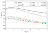 |
Fig. 1. Initial equilibrium velocity dispersion profile of the simulated UDG, computed by solving Jeans equation and taking into account the external field at the launch radius. For comparison, the solid black line corresponds to MOND in isolation, while the dotted light gray line shows the Newtonian prediction. The EFE decreases the velocity dispersion from the isolated MOND prediction, making the profile closer to the Newtonian prediction. |
In order to understand the effect of tides, we first calculated the tidal susceptibility as:
 (2)
(2)
where r1/2 ≈ (4/3)Re is the de-projected half mass radius and r2 is the Roche lobe radius perpendicularly to the axis linking the centre of the cluster and the UDG. The latter radius, r2, is calculated using the inner Lagrange point, r1, which is itself obtained by numerically solving the equation equating the UDG internal gravity with the tidal force (see Appendix B of Freundlich et al. 2022 for a complete derivation). For simulated UDGs as a function of distance from the centre of the cluster, Fig. 2 shows η, which is significant at small cluster-centric radii (< 2 Mpc).
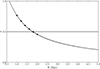 |
Fig. 2. Tidal susceptibility, η, derived from Eq. (2) as a function of distance from the cluster centre. The solid black points mark the tidal susceptibility at the distances where the UDGs were launched. Points above the horizontal η = 0.5 line are expected to be at least partially affected by tides. |
In Freundlich et al. (2022), the measured line-of-sight (los) velocity dispersions of Coma cluster UDGs were found to be in relatively good agreement with the MOND prediction in isolation. Therefore, we chose to compare the los (along the z-axis of the cluster) velocity dispersions, σlos, of the simulated UDGs with the prediction of MOND in isolation. After extracting all the output particle data using EXTRACT_POR, we subtracted the barycentre in position and velocities of all the particles at each snapshot. This subtraction allows us to calculate quantities in the rest frame of the UDGs and reduces the effect of numerical drift. At each snapshot, we constructed annuli of 0.25 kpc up to a projected radius of 5 kpc, which corresponds approximately to the distance of the furthest velocity dispersion measurement in DF44 (van Dokkum et al. 2019). However, we note that the typical radius in the observed sample within which we have data for most UDGs of the Coma cluster is of the order of 2 kpc or less. The los velocity dispersion is calculated in each bin with the unbiased estimator of the standard deviation:
 (3)
(3)
where N is the total number of particles in a given bin. For the UDGs to completely experience the effect of tides, we let them make at least one pericentric passage on their orbit. We also considered the UDGs at apocentres since they spend a longer time close to apocentre than to pericentre, except for the case of circular orbits where we analysed the last snapshot of the simulation.
The theoretical los velocity dispersion in the MOND context was derived from Sérsic fits of the surface density maps in the (x, y) plane using GALFIT (Peng et al. 2010) to emulate observational studies such as that of Freundlich et al. (2022). To compute mass throughout our simulations, we generated surface density maps along the (los) z-axis of the cluster at each snapshot, we computed the isodensity contours, corresponding to a g-band surface brightness of 29.5 mag arcsec−2, in the surface brightness using M = Mg + 21.572 − 2.5 log10(L⊙/pc2); here, Mg, and L⊙ are the absolute g-band magnitude and luminosity of the Sun. We adopted a mass-to-light ratio of 1 to convert the luminosity into mass. The 29.5 mag arcsec−2 is motivated by possible upcoming surveys with the Euclid Visual instrument (Borlaff & Gómez-Alvarez 2022). It is important to note that the mass of the UDG varies along the simulation, since we only considered the mass enclosed within the 29.5 surface brightness contour. In Figs. 3 and 4, we illustrate the typical evolution of UDGs along the simulation in terms of projected surface density maps and los velocity dispersion. We note that in all surface density maps, the observable parts of the galaxies within the 29.5 mag arcsec−2 threshold look relatively relaxed, implying that that our current observational view of such galaxies may be limited due to sensitivity; however, future deeper images may reveal that the outer parts of UDGs are severely tidally distorted. We deprojected the 2D best-fit Sérsic profile, as indicated in Section 2, using the semi-analytical approximation by Lima Neto et al. (1999) and the update by Márquez et al. (2000). We then computed the radial velocity dispersion from the Jeans equation assuming isotropy and converted it into the expected los velocity dispersion by projecting the velocity ellipsoid along the los (cf. Freundlich et al. 2022, Section 3.2.1, as well as Binney & Mamon 1982 and Mamon & Łokas 2005).
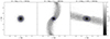 |
Fig. 3. Projected surface density maps of simulated UDGs. Left: UDG launched from R = 1 Mpc with an eccentricity e = 0 after 0.1 Gyr. Middle: Same UDG after 5 Gyr, with tidal tails. Right: UDG launched from R = 1.4 Mpc with e = 0.99 after 3.1 Gyr. In all panels, the blue contour corresponds to a surface brightness threshold of 29.5 mag arcsec−2. |
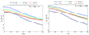 |
Fig. 4. Evolution of the los velocity dispersion (σlos) of the two simulated UDGs shown in Fig. 3. Left: UDG launched from R = 1 Mpc on a circular orbit with an eccentricity e = 0. Right: UDG launched from R = 1.4 Mpc on a radial orbit with e = 0.99. |
We derived the theoretical los velocity dispersion both in isolation (hereafter, σiso) and in the presence of an external field, σEFE. Figure 5 shows the ratio of the simulated σlos, measured with Eq. (3), to the isolated MOND theoretical prediction, σiso. The main result here is that the σlos profiles of UDGs on all orbits remain significantly below the isolated MOND prediction, indicating that tides do not increase the σlos from their initial equilibrium values (within the external field from the cluster) up to the isolated MOND prediction. Nevertheless, UDGs launched from 1 and 1.2 Mpc have rising σlos profiles that become steeper as a function of eccentricity, indicating that the outskirts are significantly affected by tides, but not enough to reach the isolated MOND prediction. To check how much heating is produced with respect to the equilibrium prediction within the external field of the cluster, σEFE, the ratio σlos/σEFE is plotted in Fig. 6. In all cases, the latter ratio in the inner parts of the UDG remains close to 1, especially for low-eccentricity orbits (this also justifies a posteriori our chosen analytical prescription for the internal gravitational field in the presence of an EFE). This shows that the inner part of the UDG is in equilibrium within the EFE, while the outer parts are not, due to tides, although not enough compared to observations.
 |
Fig. 5. Ratio between the line-of-sight velocity dispersion (σlos) of the simulated UDGs at apocentre and the corresponding expected isolated MOND prediction (σiso) as a function of radius. The six panels are arranged in the order of increasing eccentricity of the orbits of the launched UDGs, and the six different curves are colored based on the initial launch distance of the UDGs. The horizontal black line corresponds to σlos = σiso. The stellar velocity dispersion of observed Coma cluster UDGs are generally within 30% of σlos given their uncertainties (cf. Table 1 and Fig. 4 of Freundlich et al. 2022), a regime that no simulated UDG reaches. |
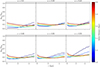 |
Fig. 6. Same as Fig. 5 but for the ratio between σlos and σEFE the Jeans equilibrium MOND prediction with EFE. The outskirts of the simulated UDGs are affected by tides but not enough to reach σiso. |
3.2. First infall onto the cluster?
Our second set of simulations of UDGs launched from 10–14 Mpc on radial orbits is meant to test whether UDGs on their first infall may not have time to equilibrate themselves with the EFE and could thus retain the velocity dispersion they had in isolation. As can be seen in Fig. 1, the velocity dispersion in equilibrium at 10 Mpc is indeed close to that expected in isolation, reaching 90% of the isolated MOND velocity dispersion in the central parts. Since it takes ∼6 Gyr for a UDG to fall towards the central 3 Mpc, we estimate that ∼166 UDGs have to be accreted per Gyr to reach the number of observed UDG candidates in the Coma cluster (∼103Bautista et al. 2023; Zaritsky et al. 2019; Yagi et al. 2016; Koda et al. 2015). Figure 7 shows the evolution of one such UDG, while Fig. 8 shows the ratio of σlos/σiso and σlos/σEFE at different times for a UDG launched from 10 Mpc on a radial orbit with an eccentricity e = 0.99. It shows that from launch to pericentre the velocity dispersion decreases, especially towards the outskirts, but not sufficiently to be in equilibrium with the EFE; close to pericentre, the velocity dispersion reaches more than four times its equilibrium value under the EFE. After pericentre, the UDG undergoes tidal heating with an increase of the velocity dispersion, especially at its centre, and it starts to equilibrate with the EFE in the outskirts. We note that this central increase of the velocity dispersion may be precisely in line with some of the velocity dispersion profiles of Coma cluster UDGs reported by Chilingarian et al. (2019, cf. also Freundlich et al. 2022, Fig. 4). Consequently, UDGs on their first infall could retain the relatively high velocity dispersion they had in isolation, but they equilibrate with the EFE after pericentre passage.
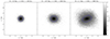 |
Fig. 7. Projected surface density maps of a UDG launched from R = 10 Mpc on a radial orbit with an eccentricity of e = 0.99 at different times. As in Fig. 3, the blue contours correspond to a surface brightness threshold of 29.5 mag arcsec−2. |
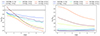 |
Fig. 8. Evolution of the ratios between the los velocity dispersion (σlos) and that predicted by MOND in isolation (σiso, left panel) and including the EFE (σEFE, right panel) for a simulated UDG launched on a radial orbit (e = 0.99) from 10 Mpc from the cluster centre. The UDG reaches pericentre around 4 Gyr. Its velocity dispersion decreases until pericentre passage (cf. σlos/σiso), however without equilibrating with the EFE (cf. σlos/σEFE), and it undergoes tidal heading after pericentre passage. Numbers in the legend indicate the simulation time and the distance from the cluster centre. |
If cluster UDGs are indeed on their first infall, their observed distribution places relatively strong constraints on their assembly history. A possibility would be that they fell together onto the cluster along cosmic filaments, as suggested by several observations (van Dokkum et al. 2019; Zaritsky et al. 2019). To illustrate this scenario, we considered a population of UDGs falling onto the cluster from 10–14 Mpc with an initial inward radial velocity of 100 km/s, which corresponds to the lower bound of average kinetic bulk flow velocities in cosmic filaments (e.g. Kraljic et al. 2019). We then followed this population as it falls towards the cluster centre. Figure 9 displays the evolution of this UDG population, whose initial distribution was specifically chosen so that its final distribution would be comparable to the observed one. It shows that with an initial cylindrical density distribution within filaments that would be almost flat, with a slight increase towards the cluster centre, such an accretion event almost 8 Gyr ago would allow for the recoverery of a distribution very similar to that of the observed Coma cluster UDGs; notably, indicating whether they came together from a cosmic filament. However, the observed distribution of UDGs is isotropic and would require at least a few such filamentary accretions at a roughly similar time for this scenario to work. This radial infall scenario is therefore the only viable scenario for explaining the kinematics of UDGs in MOND, if they do indeed have baryonic masses, as estimated observationally.
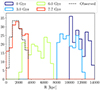 |
Fig. 9. Evolution of a UDG population launched between 10 and 14 Mpc with an inward velocity of 100 km/s, which approximately recovers the observed UDG distribution after 7.7 Gyr. |
4. Conclusion
Ultra-diffuse galaxies (UDGs) in clusters provide a testing ground for modified Newtonian dynamics (MOND) and its external field effect (EFE) given their low internal gravitational acceleration and the presence of an external field. Previous works have shown that the velocity dispersion of Coma cluster UDGs are in line with the MOND prediction in isolation, but in tension with the EFE (Freundlich et al. 2022). This result may either contradict MOND or point towards a yet-to-be found theory underpinning the MOND phenomenology, in which the EFE would be screened inside clusters. In the classical MOND context, the tension could however be alleviated if the Coma cluster UDGs had much higher baryonic mass than currently estimated, if these UDGs were heated by tides, or if they fell recently onto the cluster such that they retained part of the high velocity dispersion they had in isolation.
Here, we investigated the latter two possibilities by running N-body simulations of UDGs in a cluster potential using the ‘Phantom of Ramses’ (POR; Lüghausen et al. 2015; Nagesh et al. 2021) patch of the adaptive mesh refinement code RAMSES (Teyssier 2002). In order to eliminate spurious noise due to discrete cluster particles, we implemented an analytical external density within the POR context for the first time, which is publicly available here4. First, to test whether tides could heat up UDGs in the MOND context, we simulated UDGs on different orbits with initial radii between 1 and 2 Mpc from the cluster centre. We show that if UDGs are initially at equilibrium within the cluster external field, tides are not sufficient to increase their velocity dispersions to values as high as those observed (Section 3.1).
Then, to test whether UDGs on first infall could retain their high velocity dispersion, we simulated UDGs falling on radial orbits towards the cluster centre from distances of 10–14 Mpc. We show that such UDGs on their first radial infall onto the cluster may retain their high velocity dispersions without being destroyed until their first pericentric passage (Section 3.2). Hence, without alterations such as a screening of the EFE in galaxy clusters or higher baryonic mass, UDGs must be out-of-equilibrium objects on their first infall onto the cluster in the MOND context.
We stress that this work relies on different assumptions and simplifications. In particular, we only considered tidal forces from a smooth cluster potential, while actual clusters host substructures and other galaxies that can also influence the dynamics of UDGs and contribute to increasing their velocity dispersion or to accelerate their disruption. We further assumed initial conditions where the galaxies were already ultra-diffuse, while UDGs can in principle form through tidal heating in clusters (e.g. Jiang et al. 2019) or ram-pressure striping of gas-rich dwarf (e.g Grishin et al. 2021). The expansion of the stellar distribution is however expected to be accompanied by a decrease of the velocity dispersion during the relaxation phase if energy is conserved. We relied on the QUMOND formalism, as implemented in POR, and estimated the EFE with an analytical formula derived and tested in this context. Finally, we carried out pure N-body simulations without taking into account any possible gaseous component, including the effect of ram-pressure stripping in the radial infall scenario. It is also important to note that our simulation setup does not consider Hubble expansion of the Universe or mass growth of the Coma cluster with time, which can slow down the infall of the UDGs and moderate the EFE. However, both effects are not expected to affect the qualitative conclusions of the present work. Modelling this scenario would require a reliance on a specific formalism, such as the spherical top-hat collapse model of Malekjani et al. (2009) or on cosmological simulations in the MOND context. Finally, the framework developed in the current work could also be applied in the future to dwarf spheroidal satellites in the Local Group.
The POR package, extraction software, and other relevant algorithms are available at https://bitbucket.org/SrikanthTN/bonnPoR/src/master/, along with a POR manual to setup, run, and analyse isolated disc galaxy simulations in MOND (Nagesh et al. 2021).
This patch implements an analytic density profile of the Coma cluster in both MOND and Newtonian framework, and is available here: https://github.com/SrikanthNagesh/Coma_analytic_density_PoR
For a UDG on a circular orbit at 10 Mpc from the cluster centre, where the tidal heating is negligible, the velocity dispersions remain very close to the initial setup after launching the simulation, thereby validating the adopted EFE formula at equilibrium.
This patch implements an analytic density profile of the Coma cluster in both MOND and Newtonian framework, and is available here: https://github.com/SrikanthNagesh/Coma_analytic_density_PoR
Acknowledgments
STN thanks Gary Mamon, Nicolas Martin, Raphael Errani, Francoise Combes, and Jin Koda for useful discussions. STN, JF, BF and RI acknowledge funding from the European Research Council (ERC) under the European Union’s Horizon 2020 research and innovation program (grant agreement No. 834148). MB acknowledges partial support from UK Science and Technology Facilities Council grant ST/V000861/1 and hospitality from University of St Andrews during the visit. OM is grateful to the Swiss National Science Foundation for financial support under the grant number PZ00P2_202104.
References
- Amorisco, N. C., & Loeb, A. 2016, MNRAS, 459, L51 [NASA ADS] [CrossRef] [Google Scholar]
- Angus, G. W., Famaey, B., & Buote, D. A. 2008, MNRAS, 387, 1470 [CrossRef] [Google Scholar]
- Angus, G. W., Diaferio, A., & Kroupa, P. 2011, MNRAS, 416, 1401 [NASA ADS] [CrossRef] [Google Scholar]
- Angus, G. W., Diaferio, A., Famaey, B., & van der Heyden, K. J. 2013, MNRAS, 436, 202 [NASA ADS] [CrossRef] [Google Scholar]
- Asencio, E., Banik, I., Mieske, S., et al. 2022, MNRAS, 515, 2981 [CrossRef] [Google Scholar]
- Banik, I., & Zhao, H. 2018, MNRAS, 473, 419 [NASA ADS] [CrossRef] [Google Scholar]
- Banik, I., & Zhao, H. 2022, Symmetry, 14, 1331 [NASA ADS] [CrossRef] [Google Scholar]
- Banik, I., Thies, I., Candlish, G., et al. 2020, ApJ, 905, 135 [NASA ADS] [CrossRef] [Google Scholar]
- Banik, I., Thies, I., Truelove, R., et al. 2022, MNRAS, 513, 129 [NASA ADS] [CrossRef] [Google Scholar]
- Bautista, J. M., Koda, J., Komiyama, Y., et al. 2022, Am. Astron. Soc. Meeting Abstr., 54, 123.07 [Google Scholar]
- Bautista, J. M. G., Koda, J., Yagi, M., Komiyama, Y., & Yamanoi, H. 2023, ApJS, 267, 10 [NASA ADS] [CrossRef] [Google Scholar]
- Beasley, M. A., & Trujillo, I. 2016, ApJ, 830, 23 [CrossRef] [Google Scholar]
- Begeman, K. G., Broeils, A. H., & Sanders, R. H. 1991, MNRAS, 249, 523 [Google Scholar]
- Bekenstein, J. D. 2004, Phys. Rev. D, 70, 083509 [Google Scholar]
- Bekenstein, J., & Milgrom, M. 1984, ApJ, 286, 7 [NASA ADS] [CrossRef] [Google Scholar]
- Bennet, P., Sand, D. J., Zaritsky, D., et al. 2018, ApJ, 866, L11 [NASA ADS] [CrossRef] [Google Scholar]
- Bílek, M., Thies, I., Kroupa, P., & Famaey, B. 2018, A&A, 614, A59 [Google Scholar]
- Bílek, M., Müller, O., & Famaey, B. 2019a, A&A, 627, L1 [NASA ADS] [CrossRef] [EDP Sciences] [Google Scholar]
- Bílek, M., Samurović, S., & Renaud, F. 2019b, A&A, 625, A32 [Google Scholar]
- Bílek, M., Fensch, J., Ebrová, I., et al. 2022, A&A, 660, A28 [NASA ADS] [CrossRef] [EDP Sciences] [Google Scholar]
- Binney, J. 2008, Galactic Dynamics: Second Edition (Princeton University Press) [CrossRef] [Google Scholar]
- Binney, J., & Mamon, G. A. 1982, MNRAS, 200, 361 [Google Scholar]
- Blanchet, L., & Skordis, C. 2024, ArXiv e-prints [arXiv:2404.06584] [Google Scholar]
- Brada, R., & Milgrom, M. 1995, MNRAS, 276, 453 [Google Scholar]
- Brada, R., & Milgrom, M. 1999, ApJ, 519, 590 [NASA ADS] [CrossRef] [Google Scholar]
- Brada, R., & Milgrom, M. 2000, ApJ, 531, L21 [NASA ADS] [CrossRef] [Google Scholar]
- Candlish, G. N., Smith, R., & Fellhauer, M. 2015, MNRAS, 446, 1060 [NASA ADS] [CrossRef] [Google Scholar]
- Candlish, G. N., Smith, R., Jaffé, Y., & Cortesi, A. 2018, MNRAS, 480, 5362 [NASA ADS] [CrossRef] [Google Scholar]
- Chae, K.-H., Lelli, F., Desmond, H., et al. 2020, ApJ, 904, 51 [NASA ADS] [CrossRef] [Google Scholar]
- Chae, K.-H., Desmond, H., Lelli, F., McGaugh, S. S., & Schombert, J. M. 2021, ApJ, 921, 104 [NASA ADS] [CrossRef] [Google Scholar]
- Chilingarian, I. V., Afanasiev, A. V., Grishin, K. A., Fabricant, D., & Moran, S. 2019, ApJ, 884, 79 [NASA ADS] [CrossRef] [Google Scholar]
- de Blok, W. J. G., & McGaugh, S. S. 1997, MNRAS, 290, 533 [NASA ADS] [CrossRef] [Google Scholar]
- Desmond, H., Hees, A., & Famaey, B. 2024, MNRAS, 530, 1781 [CrossRef] [Google Scholar]
- Di Cintio, A., Brook, C. B., Dutton, A. A., et al. 2017, MNRAS, 466, L1 [NASA ADS] [CrossRef] [Google Scholar]
- Di Teodoro, E. M., Posti, L., Fall, S. M., et al. 2023, MNRAS, 518, 6340 [Google Scholar]
- Eappen, R., Kroupa, P., Wittenburg, N., Haslbauer, M., & Famaey, B. 2022, MNRAS, 516, 1081 [NASA ADS] [CrossRef] [Google Scholar]
- Emsellem, E., van der Burg, R. F. J., Fensch, J., et al. 2019, A&A, 625, A76 [NASA ADS] [CrossRef] [EDP Sciences] [Google Scholar]
- Euclid Collaboration (Borlaff, A. S., et al.) 2022, A&A, 657, A92 [NASA ADS] [CrossRef] [EDP Sciences] [Google Scholar]
- Famaey, B., & Binney, J. 2005, MNRAS, 363, 603 [NASA ADS] [CrossRef] [Google Scholar]
- Famaey, B., & McGaugh, S. S. 2012, Liv. Rev. Relat., 15, 10 [Google Scholar]
- Famaey, B., Bruneton, J.-P., & Zhao, H. 2007, MNRAS, 377, L79 [NASA ADS] [CrossRef] [Google Scholar]
- Famaey, B., McGaugh, S., & Milgrom, M. 2018, MNRAS, 480, 473 [NASA ADS] [CrossRef] [Google Scholar]
- Fosbury, R. A. E., Mebold, U., Goss, W. M., & Dopita, M. A. 1978, MNRAS, 183, 549 [NASA ADS] [CrossRef] [Google Scholar]
- Freundlich, J., Dekel, A., Jiang, F., et al. 2020a, MNRAS, 491, 4523 [NASA ADS] [CrossRef] [Google Scholar]
- Freundlich, J., Jiang, F., Dekel, A., et al. 2020b, MNRAS, 499, 2912 [NASA ADS] [CrossRef] [Google Scholar]
- Freundlich, J., Famaey, B., Oria, P.-A., et al. 2022, A&A, 658, A26 [NASA ADS] [CrossRef] [EDP Sciences] [Google Scholar]
- Gentile, G., Famaey, B., & de Blok, W. J. G. 2011, A&A, 527, A76 [NASA ADS] [CrossRef] [EDP Sciences] [Google Scholar]
- Ghari, A., Famaey, B., Laporte, C., & Haghi, H. 2019, A&A, 623, A123 [NASA ADS] [CrossRef] [EDP Sciences] [Google Scholar]
- Greco, J. P., Greene, J. E., Strauss, M. A., et al. 2018, ApJ, 857, 104 [NASA ADS] [CrossRef] [Google Scholar]
- Grishin, K. A., Chilingarian, I. V., Afanasiev, A. V., et al. 2021, Nat. Astron., 5, 1308 [NASA ADS] [CrossRef] [Google Scholar]
- Haghi, H., Amiri, V., Hasani Zonoozi, A., et al. 2019a, ApJ, 884, L25 [NASA ADS] [CrossRef] [Google Scholar]
- Haghi, H., Kroupa, P., Banik, I., et al. 2019b, MNRAS, 487, 2441 [CrossRef] [Google Scholar]
- Haslbauer, M., Dabringhausen, J., Kroupa, P., Javanmardi, B., & Banik, I. 2019, A&A, 626, A47 [NASA ADS] [CrossRef] [EDP Sciences] [Google Scholar]
- Hees, A., Famaey, B., Angus, G. W., & Gentile, G. 2016, MNRAS, 455, 449 [NASA ADS] [CrossRef] [Google Scholar]
- Janowiecki, S., Leisman, L., Józsa, G., et al. 2015, ApJ, 801, 96 [NASA ADS] [CrossRef] [Google Scholar]
- Jiang, F., Dekel, A., Freundlich, J., et al. 2019, MNRAS, 487, 5272 [CrossRef] [Google Scholar]
- Karachentsev, I. D., Karachentseva, V. E., Suchkov, A. A., & Grebel, E. K. 2000, A&AS, 145, 415 [NASA ADS] [CrossRef] [EDP Sciences] [Google Scholar]
- Koch, A., Burkert, A., Rich, R. M., et al. 2012, ApJ, 755, L13 [Google Scholar]
- Koda, J., Yagi, M., Yamanoi, H., & Komiyama, Y. 2015, ApJ, 807, L2 [NASA ADS] [CrossRef] [Google Scholar]
- Kraljic, K., Pichon, C., Dubois, Y., et al. 2019, MNRAS, 483, 3227 [Google Scholar]
- Kroupa, P., Haghi, H., Javanmardi, B., et al. 2018, Nature, 561, E4 [CrossRef] [Google Scholar]
- Leisman, L., Haynes, M. P., Janowiecki, S., et al. 2017, ApJ, 842, 133 [NASA ADS] [CrossRef] [Google Scholar]
- Lelli, F., McGaugh, S. S., Schombert, J. M., & Pawlowski, M. S. 2017, ApJ, 836, 152 [Google Scholar]
- Lelli, F., McGaugh, S. S., Schombert, J. M., Desmond, H., & Katz, H. 2019, MNRAS, 484, 3267 [NASA ADS] [CrossRef] [Google Scholar]
- Lim, S., Côté, P., Peng, E. W., et al. 2020, ApJ, 899, 69 [CrossRef] [Google Scholar]
- Lima Neto, G. B., Gerbal, D., & Márquez, I. 1999, MNRAS, 309, 481 [Google Scholar]
- Llinares, C., Knebe, A., & Zhao, H. 2008, MNRAS, 391, 1778 [NASA ADS] [CrossRef] [Google Scholar]
- Londrillo, P., & Nipoti, C. 2009, Mem. Soc. Astron. Ital. Suppl., 13, 89 [NASA ADS] [Google Scholar]
- Lüghausen, F., Famaey, B., Kroupa, P., et al. 2013, MNRAS, 432, 2846 [CrossRef] [Google Scholar]
- Lüghausen, F., Famaey, B., & Kroupa, P. 2015, Can. J. Phys., 93, 232 [CrossRef] [Google Scholar]
- Malekjani, M., Rahvar, S., & Haghi, H. 2009, ApJ, 694, 1220 [CrossRef] [Google Scholar]
- Mamon, G. A., & Łokas, E. L. 2005, MNRAS, 363, 705 [Google Scholar]
- Marleau, F. R., Habas, R., Poulain, M., et al. 2021, A&A, 654, A105 [NASA ADS] [CrossRef] [EDP Sciences] [Google Scholar]
- Márquez, I., Lima Neto, G. B., Capelato, H., Durret, F., & Gerbal, D. 2000, A&A, 353, 873 [NASA ADS] [Google Scholar]
- Martínez-Vázquez, C. E., Monelli, M., Bono, G., et al. 2015, MNRAS, 454, 1509 [Google Scholar]
- McGaugh, S. S. 2016, ApJ, 832, L8 [NASA ADS] [CrossRef] [Google Scholar]
- McGaugh, S., & Milgrom, M. 2013, ApJ, 775, 139 [NASA ADS] [CrossRef] [Google Scholar]
- McGaugh, S. S., Schombert, J. M., Bothun, G. D., & de Blok, W. J. G. 2000, ApJ, 533, L99 [Google Scholar]
- Merritt, A., van Dokkum, P., Danieli, S., et al. 2016, ApJ, 833, 168 [NASA ADS] [CrossRef] [Google Scholar]
- Mihos, J. C., Durrell, P. R., Ferrarese, L., et al. 2015, ApJ, 809, L21 [Google Scholar]
- Mihos, J. C., Harding, P., Feldmeier, J. J., et al. 2017, ApJ, 834, 16 [Google Scholar]
- Milgrom, M. 1983a, ApJ, 270, 371 [Google Scholar]
- Milgrom, M. 1983b, ApJ, 270, 365 [Google Scholar]
- Milgrom, M. 1994, Ann. Phys., 229, 384 [NASA ADS] [CrossRef] [Google Scholar]
- Milgrom, M. 2010, MNRAS, 403, 886 [NASA ADS] [CrossRef] [Google Scholar]
- Milgrom, M., 2014, Scholarpedia, 9, 31410 [NASA ADS] [CrossRef] [Google Scholar]
- Milgrom, M. 2022, Phys. Rev. D, 106, 064060 [NASA ADS] [CrossRef] [Google Scholar]
- Müller, O., Pawlowski, M. S., Jerjen, H., & Lelli, F. 2018, Science, 359, 534 [CrossRef] [Google Scholar]
- Müller, O., Famaey, B., & Zhao, H. 2019, A&A, 623, A36 [Google Scholar]
- Müller, O., Durrell, P. R., Marleau, F. R., et al. 2021, ApJ, 923, 9 [CrossRef] [Google Scholar]
- Nagesh, S. T., Banik, I., Thies, I., et al. 2021, Can. J. Phys., 99, 607 [NASA ADS] [CrossRef] [Google Scholar]
- Nagesh, S. T., Kroupa, P., Banik, I., et al. 2023, MNRAS, 519, 5128 [NASA ADS] [CrossRef] [Google Scholar]
- Nipoti, C., Ciotti, L., & Londrillo, P. 2011, MNRAS, 414, 3298 [Google Scholar]
- Nusser, A. 2019, MNRAS, 484, 510 [CrossRef] [Google Scholar]
- Oman, K. A., Navarro, J. F., Fattahi, A., et al. 2015, MNRAS, 452, 3650 [CrossRef] [Google Scholar]
- Oria, P.-A., Famaey, B., Thomas, G. F., et al. 2021, ArXiv e-prints [arXiv:2109.10160] [Google Scholar]
- Pawlowski, M. S., Famaey, B., Merritt, D., & Kroupa, P. 2015, ApJ, 815, 19 [NASA ADS] [CrossRef] [Google Scholar]
- Peng, C. Y., Ho, L. C., Impey, C. D., & Rix, H.-W. 2010, AJ, 139, 2097 [Google Scholar]
- Prole, D. J., van der Burg, R. F. J., Hilker, M., & Davies, J. I. 2019, MNRAS, 488, 2143 [NASA ADS] [Google Scholar]
- Reiprich, T. H. 2001, Ph.D. Thesis, Max-Planck-Institut für extraterrestrische Physik, P.O. Box 1312, Garching bei München, Germany [Google Scholar]
- Renaud, F., Famaey, B., & Kroupa, P. 2016, MNRAS, 463, 3637 [NASA ADS] [CrossRef] [Google Scholar]
- Román, J., & Trujillo, I. 2017, MNRAS, 468, 703 [CrossRef] [Google Scholar]
- Sandage, A., & Binggeli, B. 1984, AJ, 89, 919 [Google Scholar]
- Sanders, R. H. 1999, ApJ, 512, L23 [NASA ADS] [CrossRef] [Google Scholar]
- Sanders, R. H. 2003, MNRAS, 342, 901 [NASA ADS] [CrossRef] [Google Scholar]
- Scott, T. C., Sengupta, C., Lagos, P., Chung, A., & Wong, O. I. 2021, MNRAS, 503, 3953 [NASA ADS] [CrossRef] [Google Scholar]
- Skordis, C., & Złośnik, T. 2020, ArXiv e-prints [arXiv:2007.00082] [Google Scholar]
- Stiskalek, R., & Desmond, H. 2023, MNRAS, 525, 6130 [NASA ADS] [CrossRef] [Google Scholar]
- Swaters, R. A., Sancisi, R., van Albada, T. S., & van der Hulst, J. M. 2009, A&A, 493, 871 [NASA ADS] [CrossRef] [EDP Sciences] [Google Scholar]
- Teyssier, R. 2002, A&A, 385, 337 [CrossRef] [EDP Sciences] [Google Scholar]
- Thomas, G. F., Famaey, B., Ibata, R., Lüghausen, F., & Kroupa, P. 2017, A&A, 603, A65 [NASA ADS] [CrossRef] [EDP Sciences] [Google Scholar]
- Thomas, G. F., Famaey, B., Ibata, R., et al. 2018, A&A, 609, A44 [NASA ADS] [CrossRef] [EDP Sciences] [Google Scholar]
- Tiret, O., & Combes, F. 2008a, A&A, 483, 719 [NASA ADS] [CrossRef] [EDP Sciences] [Google Scholar]
- Tiret, O., & Combes, F. 2008b, ASP Conf. Ser., 396, 259 [Google Scholar]
- Toloba, E., Sand, D. J., Spekkens, K., et al. 2016, ApJ, 816, L5 [Google Scholar]
- Toloba, E., Lim, S., Peng, E., et al. 2018, ApJ, 856, L31 [CrossRef] [Google Scholar]
- van Dokkum, P. G., Abraham, R., Merritt, A., et al. 2015a, ApJ, 798, L45 [NASA ADS] [CrossRef] [Google Scholar]
- van Dokkum, P. G., Romanowsky, A. J., Abraham, R., et al. 2015b, ApJ, 804, L26 [NASA ADS] [CrossRef] [Google Scholar]
- van Dokkum, P., Abraham, R., Brodie, J., et al. 2016, ApJ, 828, L6 [Google Scholar]
- van Dokkum, P., Abraham, R., Romanowsky, A. J., et al. 2017, ApJ, 844, L11 [NASA ADS] [CrossRef] [Google Scholar]
- van Dokkum, P., Danieli, S., Cohen, Y., et al. 2018, Nature, 555, 629 [Google Scholar]
- van Dokkum, P., Wasserman, A., Danieli, S., et al. 2019, ApJ, 880, 91 [Google Scholar]
- Venhola, A., Peletier, R., Laurikainen, E., et al. 2017, A&A, 608, A142 [NASA ADS] [CrossRef] [EDP Sciences] [Google Scholar]
- Wasserman, A., van Dokkum, P., Romanowsky, A. J., et al. 2019, ApJ, 885, 155 [NASA ADS] [CrossRef] [Google Scholar]
- Wittenburg, N., Kroupa, P., & Famaey, B. 2020, ApJ, 890, 173 [NASA ADS] [CrossRef] [Google Scholar]
- Wittenburg, N., Kroupa, P., Banik, I., Candlish, G., & Samaras, N. 2023, MNRAS, 523, 453 [NASA ADS] [CrossRef] [Google Scholar]
- Wittmann, C., Lisker, T., Ambachew Tilahun, L., et al. 2017, MNRAS, 470, 1512 [Google Scholar]
- Yagi, M., Koda, J., Komiyama, Y., & Yamanoi, H. 2016, ApJS, 225, 11 [CrossRef] [Google Scholar]
- Zaritsky, D., Donnerstein, R., Dey, A., et al. 2019, ApJS, 240, 1 [Google Scholar]
All Figures
|
Fig. 1. Initial equilibrium velocity dispersion profile of the simulated UDG, computed by solving Jeans equation and taking into account the external field at the launch radius. For comparison, the solid black line corresponds to MOND in isolation, while the dotted light gray line shows the Newtonian prediction. The EFE decreases the velocity dispersion from the isolated MOND prediction, making the profile closer to the Newtonian prediction. |
| In the text | |
|
Fig. 2. Tidal susceptibility, η, derived from Eq. (2) as a function of distance from the cluster centre. The solid black points mark the tidal susceptibility at the distances where the UDGs were launched. Points above the horizontal η = 0.5 line are expected to be at least partially affected by tides. |
| In the text | |
|
Fig. 3. Projected surface density maps of simulated UDGs. Left: UDG launched from R = 1 Mpc with an eccentricity e = 0 after 0.1 Gyr. Middle: Same UDG after 5 Gyr, with tidal tails. Right: UDG launched from R = 1.4 Mpc with e = 0.99 after 3.1 Gyr. In all panels, the blue contour corresponds to a surface brightness threshold of 29.5 mag arcsec−2. |
| In the text | |
|
Fig. 4. Evolution of the los velocity dispersion (σlos) of the two simulated UDGs shown in Fig. 3. Left: UDG launched from R = 1 Mpc on a circular orbit with an eccentricity e = 0. Right: UDG launched from R = 1.4 Mpc on a radial orbit with e = 0.99. |
| In the text | |
|
Fig. 5. Ratio between the line-of-sight velocity dispersion (σlos) of the simulated UDGs at apocentre and the corresponding expected isolated MOND prediction (σiso) as a function of radius. The six panels are arranged in the order of increasing eccentricity of the orbits of the launched UDGs, and the six different curves are colored based on the initial launch distance of the UDGs. The horizontal black line corresponds to σlos = σiso. The stellar velocity dispersion of observed Coma cluster UDGs are generally within 30% of σlos given their uncertainties (cf. Table 1 and Fig. 4 of Freundlich et al. 2022), a regime that no simulated UDG reaches. |
| In the text | |
|
Fig. 6. Same as Fig. 5 but for the ratio between σlos and σEFE the Jeans equilibrium MOND prediction with EFE. The outskirts of the simulated UDGs are affected by tides but not enough to reach σiso. |
| In the text | |
|
Fig. 7. Projected surface density maps of a UDG launched from R = 10 Mpc on a radial orbit with an eccentricity of e = 0.99 at different times. As in Fig. 3, the blue contours correspond to a surface brightness threshold of 29.5 mag arcsec−2. |
| In the text | |
|
Fig. 8. Evolution of the ratios between the los velocity dispersion (σlos) and that predicted by MOND in isolation (σiso, left panel) and including the EFE (σEFE, right panel) for a simulated UDG launched on a radial orbit (e = 0.99) from 10 Mpc from the cluster centre. The UDG reaches pericentre around 4 Gyr. Its velocity dispersion decreases until pericentre passage (cf. σlos/σiso), however without equilibrating with the EFE (cf. σlos/σEFE), and it undergoes tidal heading after pericentre passage. Numbers in the legend indicate the simulation time and the distance from the cluster centre. |
| In the text | |
|
Fig. 9. Evolution of a UDG population launched between 10 and 14 Mpc with an inward velocity of 100 km/s, which approximately recovers the observed UDG distribution after 7.7 Gyr. |
| In the text | |
Current usage metrics show cumulative count of Article Views (full-text article views including HTML views, PDF and ePub downloads, according to the available data) and Abstracts Views on Vision4Press platform.
Data correspond to usage on the plateform after 2015. The current usage metrics is available 48-96 hours after online publication and is updated daily on week days.
Initial download of the metrics may take a while.