| Issue |
A&A
Volume 691, November 2024
|
|
|---|---|---|
| Article Number | A21 | |
| Number of page(s) | 11 | |
| Section | Stellar structure and evolution | |
| DOI | https://doi.org/10.1051/0004-6361/202450361 | |
| Published online | 28 October 2024 | |
The impact of UV spectra on searches for extremely metal-poor stars: A study for future CSST observations
1
School of Mathematics and Statistics, Shandong University, Weihai, 264209 Shandong, PR China
2
CAS Key Lab of Optical Astronomy, National Astronomical Observatories, Chinese Academy of Sciences, A20 Datun Road, Chaoyang, Beijing 100101, China
3
School of Astronomy and Space Science, University of Chinese Academy of Sciences, Beijing 100049, PR China
4
School of Physics and Technology, Nantong University, Nantong 226019, China
5
School of Mechanical, Electrical and Information Engineering, Shandong University, Weihai, 264209 Shandong, PR China
6
School of Mathematics and Statistics, Shandong University, Weihai, 264209 Shandong, PR China
⋆ Corresponding authors; buyude@sdu.edu.cn; whl1156646283@163.com
Received:
13
April
2024
Accepted:
8
August
2024
Extremely metal-poor (EMPs, [Fe/H] < −3.0) and carbon-enhanced EMP (CE-EMP, [Fe/H] < −3.0 and [C/Fe]> + 1.0) stars are crucial for understanding the chemical evolution and early formation of the galaxies. Current research on EMP stars is limited by small samples, and ultraviolet (UV) band spectra are lacking. The China Space Station Telescope (CSST) will provide high-quality, low-resolution spectra across wavelengths from near-ultraviolet to near-infrared, with a limiting magnitude of about 21 mag. These will help in identifying EMPs and CE-EMP candidates in the distant Milky Way and nearby galaxies. The present study first uses the simulated CSST spectra to quantitatively evaluate the contribution of UV band spectra in predicting [Fe/H], [α/Fe], and [C/Fe]. The results indicate that UV band spectra reduce the mean absolute error by 0.04, 0.04, and 0.03, respectively, with a σ of 0.02, 0.03, and 0.04, respectively. Further spectral analysis reveals that the EMP stars show unique spectral-line features in the UV band, with significant differences compared to stars of higher metallicity, which could help in identifying EMP stars. Additionally, we tested the impact of UV band spectra on identifying EMP and CE-EMP stars at different noise levels and find that models including UV band spectra improve the identification of EMP and CE-EMP stars in terms of accuracy, recall, and F1 score. At low signal-to-noise ratio (S/N), the model including the UV band achieves a recall of 0.94, significantly higher than the model without the UV band (Recall = 0.48), doubling the capability to identify EMP stars. As the S/N increases, the inclusion of the UV band maintains high recall. This suggests that UV spectra in future large surveys could reduce the risk of missing potentially interesting stellar candidates, ensuring a more comprehensive identification of all possible EMP and CE-EMP star candidates.
Key words: methods: data analysis / methods: statistical / techniques: spectroscopic / astrometry / ultraviolet: stars
© The Authors 2024
 Open Access article, published by EDP Sciences, under the terms of the Creative Commons Attribution License (https://creativecommons.org/licenses/by/4.0), which permits unrestricted use, distribution, and reproduction in any medium, provided the original work is properly cited.
This article is published in open access under the Subscribe to Open model. Subscribe to A&A to support open access publication.
1. Introduction
The stars in the Milky Way with very metal-poor (VMP, [Fe/H] < −2.0) and extremely metal-poor stars (EMP, [Fe/H] < −3.0), carry the chemical fingerprints of gas from the early Universe, which are essential for unveiling the nature of the first generation of stars, known as Population III stars (Beers & Christlieb 2005; Frebel & Norris 2015). Among the EMP stars, many are carbon-enhanced stars with carbon-to-iron ratios [C/Fe] > +1.0, which are known as carbon-enhanced metal-poor stars (CEMP). Their fraction increases with decreasing metallicity: they comprise approximately 30% of all stars with [Fe/H] < −2.0, 60% of those with [Fe/H] < −3.0, and 80% of all stars with [Fe/H] < −4.0 (e.g. Lucatello et al. 2006; Placco et al. 2014; Yoon et al. 2018). By analysing the chemical abundances of EMP and CEMP stars, we can enhance our understanding of early nucleosynthesis processes and constrain the properties of early stars such as mass, rotation rates, mixing processes, explosion energies, remnant masses (whether neutron stars or black holes), and thermohaline convection (e.g. Heger & Woosley 2010; Limongi & Chieffi 2012; Wanajo 2018; Jones et al. 2019; Ishigaki et al. 2021). These studies can also help us to elucidate the early formation and evolution of the Milky Way (e.g. Hawkins et al. 2015; Das et al. 2020; Helmi 2020; Horta et al. 2021; Belokurov & Kravtsov 2022; Conroy et al. 2022; Rix et al. 2022).
However, metal-poor stars are relatively rare in the Milky Way, constituting less than 0.1% of the total stellar population of the Galaxy (see Starkenburg et al. 2017; El-Badry et al. 2018; Li et al. 2018; Placco et al. 2018; Chiti et al. 2021). The EMP stars are especially scarce, and the search for them typically involves the following steps: (i) a broad survey is conducted to filter potential metal-poor star candidates; (ii) medium-resolution spectroscopic follow-up observations are employed to verify which candidates are indeed metal-poor stars; and (iii) the most valuable stars identified in the second step are subjected to high-resolution spectroscopic analysis. Spectroscopic surveys are particularly effective in this process, not only because they identify a higher proportion of genuine metal-poor stars among the candidates but also because the samples obtained in this manner are dynamically unbiased, offering significant advantages over those selected solely based on proper motion (e.g. Beers & Christlieb 2005; Hughes et al. 2022; Da Costa et al. 2023). Moreover, large astronomical surveys, such as the Sloan Digital Sky Survey and its extensions for understanding and evolving the Milky Way (SDSS/SEGUE; York et al. 2000; Yanny et al. 2009; Rockosi et al. 2022); the Large Sky Area Multi-Object Fiber Spectroscopic Telescope (LAMOST; Deng et al. 2012; Liu et al. 2014); the Gaia-ESO Public Spectroscopic Survey (Gilmore et al. 2022; Randich et al. 2022); the Apache Point Observatory Galactic Evolution Experiment (APOGEE; Majewski et al. 2017); the Radial Velocity Experiment (RAVE; Steinmetz et al. 2006); and Galactic Archaeology with HERMES (GALAH; Buder et al. 2018), have identified thousands of metal-poor stars by observing their medium-resolution spectra and estimating their metallicity. However, the sample size remains far from sufficient for the study of early formation and evolution of our Galaxy.
In addition to the limitations of small sample sizes, current research on metal-poor stars generally does not take into consideration or is restricted by the ultraviolet (UV) band. Sneden et al. (2023) pointed out that iron-group elements exhibit numerous transitions in the vacuum UV region, especially within the near-ultraviolet (NUV) wavelength range of 3000–4000 Å. This band not only facilitates the detection of absorption lines of iron-group elements, crucial for the accurate determination of metallicity in stars, but also offers information on the abundance of α-elements (such as oxygen, magnesium, silicon, etc.) and other significant elements present in the atmospheres of stars. Lu et al. (2024) also demonstrated the potential of the NUV band in estimating metallicity. By combining data from the GALEX GR6+7 All-sky Imaging Survey and Gaia Early Data Release 3, along with stellar parameters from the SAGA and PASTEL catalogues, these latter authors revealed a strong dependency of metallicity on the NUV band and showed that information from this band can effectively provide a more complete census of VMP and EMP stars with minimal influence from enhancements of C and N. However, these studies have not provided a quantitative analysis to measure the actual improvement in [Fe/H] regression accuracy when the UV band spectra are included an analysis, nor has there been a quantitative study of the contribution of the UV band in complex noise environments, especially when searching for EMP stars.
Given that stars with lower metallicity have weaker metal lines, the Hubble Space Telescope (HST), located above the terrestrial atmosphere, is able to access space UV spectroscopy, thus providing crucial supplementary information that is often challenging to obtain with ground-based telescopes. However, due to the limited receiving capacity of the HST, such observations are only feasible for a very small number of stars (Bonifacio et al. 2019). Future space telescopes equipped with more powerful gathering capabilities will be indispensable for gaining a deeper understanding of the early evolution of the Milky Way. The China Space Station Telescope (CSST) is a space telescope following the HST (Pang et al. 2022). It will be equipped with a two-metre diameter collecting area with a field of view of 1.1 deg2 in width, and will conduct photometric and slitless grating spectroscopic surveys across a large sky area of 17 500 deg2, featuring a high spatial resolution of approximately 0.15 arcseconds (Zhan 2011; Cao et al. 2018; Gong et al. 2019). The imaging survey of the CSST will cover the 255–1000 nm wavelength range from NUV to near-infrared (NIR) through seven photometric filters (NUV, u, g, r, i, z, and y). In the g band and NUV, its limiting magnitudes are 26.3 and 25.4 mag, respectively, which will extend to 27.5 and 26.7 mag for ultradeep field observations. The spectroscopic survey comprises three bands, GU (255–420 nm), GV (400–650 nm), and GI (620–1000 nm), with the aim being to provide high-quality low-resolution (R > 200) seamless spectra for hundreds of millions targets, with a limiting magnitude of about 21 mag. The observation capabilities of the CSST in the UV band and its limiting magnitudes are capable of detecting very faint celestial objects over a large area, significantly increasing the number of metal-poor star candidates. This is crucial for finding EMP stars located in distant parts of the Milky Way or nearby galaxies.
In the present study, we improved the deep learning algorithm SPT (Zhang et al. 2024a), which is designed for analysing high-dimensional spectral features. We used simulated spectral data from CSST (2550–10 000 Å) in a quantitative analysis, investigating the impact of UV band spectral features on the estimates of [Fe/H], [α/Fe], and [C/Fe]. Additionally, we quantitatively evaluated the effect of UV band spectral features on identifying EMP stars under various noise levels. We also performed quantitative tests to assess whether our method can effectively distinguish between carbon-enhanced EMP (CE-EMP) stars and carbon-normal EMP (CN-EMP) stars under these conditions. This consideration is crucial because the search for EMP and CEMP stars in real-world scenarios often occurs in noisy environments. Our goal is to ensure that our method can effectively identify target objects even under low-signal-to-noise-ratio (S/N) conditions.
The paper is organised as follows: In Sect. 2, we introduce the data used and the preprocessing steps undertaken to ensure the accuracy and reliability of the data. Section 3 provides a detailed description of the methods adopted, including model construction and evaluation metrics. Section 4 focuses on the regression analysis of [Fe/H], [α/Fe], and [C/Fe], as well as a quantitative study on the search for EMP stars, including an exploration of our ability to distinguish between CE-EMP and CN-EMP stars at different noise levels. Finally, Sect. 5 concludes the paper.
2. Data
2.1. Synthetic spectra
Given the limited availability of spectra that include the UV band, particularly for EMP stars, we used a synthetic spectral library based on PHOENIX atmospheric models (Husser et al. 2013) to simulate spectra as observed by the CSST. This approach enabled us to specifically analyse how the inclusion of the UV band data improves the identification of EMP stars in large datasets.
The PHOENIX grid encompasses a comprehensive set of synthetic spectra suitable for a wide range of spectral analyses and stellar parameter syntheses. This spectral grid was generated using the PHOENIX model atmospheres and radiative transfer code. All model atmospheres are computed assuming local thermodynamic equilibrium (LTE) and spherical geometry. For certain specific lines (such as Li I, Na I, K I, Ca I, and Ca II), non-local thermodynamic equilibrium (NLTE) effects are included, and the micro-turbulence in the model atmospheres is described using a novel, self-consistent approach. The spectra cover a broad wavelength range from the UV to the mid-infrared (MIR; 500–50 000 Å), with resolution powers of R = 500 000 for optical and NIR, while R = 100 000 for IR, with a △λ = 0.1 Å for the UV. The parameter space encompasses effective temperatures (Teff) ranging from 2300 K to 12 000 K, and surface gravity (log g) constrains the properties of early stars such as mass, rotation rates, mixing processes, explosion energies, remnant masses from 0.0 to +6.0, metallicity ([Fe/H]) from −4.0 to +1.0, and α-element abundance ([α/Fe]) from −0.2 to +1.2. This synthetic spectral library has been used in several studies, such as Kamann et al. (2016), who analysed the stars of the metal-poor globular cluster NGC 6397 in MUSE integral field spectroscopy. Wang & Luo (2019) applied machine learning techniques to analyse lower resolution spectra from LAMOST, and Zhang et al. (2024b) validated the higher sensitivity to metallicity of the NUV band due to its rich metal lines based on this dataset.
Additionally, due to the prevalence of CEMP stars at low metallicity, it is important to evaluate [C/Fe], and specifically to quantitatively test if our approach significantly differs in identifying EMP and CE-EMP stars. To this end, we additionally built a set of synthetic spectra that include [C/Fe], computed with the synthesis code SPECTRUM (Gray & Corbally 1994). SPECTRUM calculates the synthetic spectra using the ATLAS9 stellar atmosphere model grid of Castelli & Kurucz (2003), assuming LTE and a plane-parallel atmosphere. The generated synthetic spectra have a resolution of 0.01 Å. The parameter space covers 4600 K ≤ Teff ≤ 7000 K, 0.0 ≤ log g ≤ +5.0, −4.0 ≤ [Fe/H] ≤ +0.5, and −1.0 ≤ [C/Fe]≤ + 4.0. We apply the same resolution degradation and noise-addition methods described in Sects. 2.2 and 2.3, respectively, to the synthesised spectra of the two atmospheric models mentioned above.
2.2. Resolution matching
To better match the resolution of the CSST spectra, we convolved the synthetic spectra to achieve a comparable resolution (R ≈ 200). This process of reducing resolution is achieved through convolution, which involves mathematically convolving the original spectra with a resolution function (also known as the point spread function (PSF)). In this case, we used a Gaussian function as the resolution function, which simulates the broadening effect of optical instruments on incident light rays. This process results in broader spectral lines, thus reducing the resolution of the spectra. Specifically, the Gaussian function is defined as:
where μ is the centre of the Gaussian function (corresponding to the central wavelength of the spectral line), and σ is the standard deviation, which is related to the resolution of the spectroscopic instrument (R). The relationship between σ and the full width at half maximum (FWHM) is:
In practice, the FWHM is determined from the resolution R, that is,

where λ is the central wavelength. The implementation of the convolution operation includes the following steps:
(i) Wavelength grid generation: Generate a new wavelength grid based on a given resolution R. This grid is used to determine the wavelength points of the spectrum after convolution.
(ii) Convolution kernel (Gaussian function) preparation: For each point on the new wavelength grid, we calculate the FWHM based on its wavelength value and the given resolution R, and then determine the corresponding Gaussian function.
(iii) Convolution operation: For each point on the new wavelength grid, we convolve the original spectral data with the Gaussian function associated with that point, which involves slicing the original spectral data, dot-multiplying with the Gaussian kernel, and then summing the results to obtain the convolved spectral intensity value.
(iv) Parallel processing: To improve the processing speed, parallel computing methods are employed to handle the convolution operation at each wavelength point.
Figure 1 presents the spectra of one EMP model before and after the resolution-reduction process.
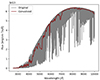 |
Fig. 1. Comparative spectral profiles pre- and post-resolution reduction for a stellar model with Teff = 3500 K, log g = +4.0, and [α/Fe]= + 3.0. The grey curve depicts the original high-resolution spectrum. The red curve illustrates the spectrum after Gaussian convolution processing, which reduces the resolution to simulate the observational effect of the CSST. The wavelength range extends from 2550 to 10 000 Å, displaying the changes from the UV to the NIR region following the resolution-degradation process. |
2.3. Add noise
After reducing the spectral resolution, we simulated the observational conditions of the CSST by adding Gaussian noise to the synthetic spectra. We fully recognise that this approach may not perfectly reflect all noise sources present in real observations. Noise in actual astronomical observations can originate from various factors, including but not limited to atmospheric disturbances, instrument noise, statistical fluctuations of photon counting, and so on. Given the complexity of accurately simulating these components, using Gaussian noise is a common and effective approach to approximating the random perturbations that affect the signal during observations.
By controlling different noise levels (i.e. S/N = 10, 20, 30), we are able to quantify the potential contribution of UV band information to improving the efficiency of identifying EMP stars under ideal conditions, systematically simulate and evaluate the search capabilities under various noise conditions, especially under low-S/N scenarios, and to provide predictions of performance under real observational conditions. In summary, although Gaussian noise may not fully replicate the actual noise observed by CSST, this approach is reasonable and necessary for the purposes of this study.
The generation of noise follows a Gaussian distribution, with the standard deviation σ(λ) determined by the formula:

where σ(λ) is the standard deviation of noise at wavelength λ, and F(λ) represents the spectral flux at that wavelength. For cases where the flux is non-positive, σ is set to a very small positive value (1 × 10⁻¹⁰) to avoid division by zero. The noise is then added to the spectrum using a Gaussian distribution centred at zero value with σ(λ) as the standard deviation, and the error estimate is updated accordingly.
Our first dataset contains a total of 27 702 spectra. We divided it into training and testing sets with an 8:2 ratio, resulting in 22 161 spectra for the training set and 5541 spectra for the testing set. The second dataset consists of 131 024 spectra, including 18 751 EMP stars and 112 273 normal stars ([Fe/H] > −3.0). Among these EMP stars, 10 411 are CE-EMP stars. We applied the same 8:2 split ratio to divide the second dataset into training and testing sets.
3. Methods
3.1. Algorithm
In the domain of spectral data analysis, the conventional convolutional neural networks (CNNs) and recurrent neural networks (RNNs) present inherent constraints. CNNs extract features through local convolution kernels, focusing primarily on local patterns, which limits their ability to capture long-range dependencies. On the other hand, RNNs, capable of processing sequential data, face issues of vanishing or exploding gradients with long sequences, and their recursive computation nature also makes them less efficient than other network structures. Considering these drawbacks, we adopted the SPT method proposed by Zhang et al. (2024a), a deep learning algorithm designed specifically for spectral data. SPT, through the design of multi-head Hadamard self attention (Multi-head HSA) operators, combines the global attention capability of self-attention mechanisms with the multi-perspective viewing ability of multi-head attention mechanisms, effectively capturing comprehensive information on the spectral data in different representation spaces, overcoming the limitations of traditional methods.
We modified the SPT method to adapt it to our research needs. As shown in Fig. 2, the embedding layer and the SPT backbone remain unchanged, continuing to serve as the foundational part for feature extraction. The MLP head is divided into two parts: one for regression on [Fe/H], [α/Fe], and [C/Fe], and the other for a binary classification task for identifying EMP and CE-EMP stars.
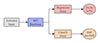 |
Fig. 2. Model architecture. At its core, the architecture comprises an embedded input layer and an SPT backbone, which together form the fundamental feature-extraction module. Building on this, the model bifurcates into two specialised branches: a regression head tasked with the precise prediction of stellar [Fe/H] and [α/Fe] indices, and a classification head designed for the binary classification of EMP and non-EMP stars. |
For different tasks, we employed specific loss functions to ensure that the model accurately learns distinct features. Specifically, the regression task utilises the SmoothL1 loss function to reduce training instability when handling outliers, thereby enhancing the robustness of the model. For the classification task of EMP stars, cross-entropy loss is used to better guide the model in discerning classification boundaries.
The optimiser chosen for the model is the Adam algorithm, which combines the advantages of Adagrad and RMSprop algorithms. It not only adaptively adjusts the learning rate for each parameter but is also suitable for optimising large-scale data and parameters. We set the initial learning rate to 0.00002 and adopted a StepDecay learning-rate decay strategy, reducing the learning rate by a decay factor gamma (set to 0.8) every 100 epochs in order to gradually decrease the learning rate and help the model converge more stably in the later stages of training. Furthermore, to avoid overfitting and enhance the generalisation capability of the model, we also incorporated an L2 regularisation term, with a weight decay coefficient set of 0.005.
3.2. Evaluation metrics for [Fe/H], [α/Fe], and [C/Fe]
In this study, we aim to determine if the inclusion of UV bands can improve the accuracy of predicting [Fe/H], [α/Fe], and [C/Fe]. We quantitatively measured this improvement using three evaluation metrics: the mean absolute error (MAE), the standard deviation (σ), and the median (M).
MAE represents the average absolute difference between the model predictions and the labels. The calculation formula is
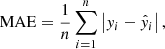
where n is the total number of samples, yi is the label of the ith sample, and  is the prediction of the model. The smaller the MAE, the higher the prediction accuracy.
Here, σ indicates the range of the distribution of model prediction errors, and is defined as
where n, yi, and  are defined as above. The smaller the σ, the higher the consistency of model predictions – that is, the better the stability of the model.
Here, M represents the median of all absolute values of prediction errors, providing a measure of the central tendency of errors that is not influenced by extreme values. The calculation formula is
where  is the absolute value of the difference between the label and the model prediction for the ith sample.
3.3. Evaluation metrics for identifying EMP and CE-EMP stars
To evaluate the impact of including UV bands on our ability to identify EMP and CE-EMP stars, we used three classification metrics: accuracy, recall, and F1 score. These metrics are commonly used for assessing the performance of binary classification models, particularly in scenarios with imbalanced datasets.
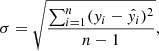
Accuracy measures the percentage of all samples that are correctly classified. A high accuracy score means that the model is effective at correctly identifying both positive (EMP or CE-EMP stars) and negative (normal or CN-EMP stars) cases. It is a crucial metric for evaluating the overall performance of a classification model and can be calculated using the following equation:
where TP refers to the number of stars that are actual EMP or CE-EMP stars and are correctly predicted as such by the model. TN is the number of stars that are actual normal or CN-EMP stars and are accurately predicted as such. FP represents the stars that are actually normal or CN-EMP stars but are incorrectly predicted as EMP or CE-EMP stars. FN is the number of stars that are actually EMP or CE-EMP stars but are mistakenly predicted as normal or CN-EMP stars.
Recall measures the proportion of actual EMP or CE-EMP stars that are correctly identified by the model. A high recall indicates that the model is effective at identifying most of the EMP or CE-EMP stars. In practical applications, it is important to maximise recall in order to ensure that as many of these rare star types as possible are correctly identified.
The recall can be derived with the following relation:
The F1 score is a comprehensive metric that balances precision and recall, evaluating the overall performance in identifying EMP or CE-EMP stars. It provides a single measure that accounts for both the accuracy and the ability to identifying these rare star types. The F1 score can be formulated as follows:
4. Results
4.1. Regression results for [Fe/H] and [α/Fe]
In our study of the impact of UV band spectra on the accuracy of predicting [Fe/H] and [α/Fe], we find that when UV band spectra are included, the predicted results for both [Fe/H] (shown in the top-left panel of Fig. 3) and [α/Fe] (shown in the top-right panel of Fig. 3) are closely clustered along the 45 degree line. This indicates a high level of agreement between the predicted and actual values. In contrast, when UV band spectra are excluded, the predicted values, although still centred around the 45 degree line, show a more dispersed density distribution, as seen in the bottom-left panel ([Fe/H]) and bottom-right panel ([α/Fe]) of Fig. 3. This dispersion is particularly noticeable for stars with low metallicity ([Fe/H]< − 3.0), suggesting an increase in prediction uncertainty. These results indicate that the lack of UV band spectra negatively impacts the prediction of [Fe/H] and [α/Fe] in stars.
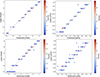 |
Fig. 3. Prediction results for [Fe/H] and [α/Fe] with and without the UV band spectra (ranging from 2550–10 000 Å and 4000–10 000 Å, respectively). The top panels compare the predicted and actual values of [Fe/H] and [α/Fe] when the UV band spectra are included. The colour intensity represents the density of data points, ranging from blue (low density) to red (high density). The dashed lines represent the identity line. The bottom panels show the prediction results without the UV band spectra. |
Table 1 indicates that, for [Fe/H] predictions, with the inclusion of the UV band data, the MAE, σ, and M are 0.04, 0.03, and −0.006; whereas without the UV band spectra, these values are 0.08, 0.05, and −0.008, respectively. The inclusion of UV band spectra notably reduces both MAE and σ, indicating an improvement in the precision and consistency of predictions. The negative values of the error median suggest that predictions are generally slightly lower than the actual values, but the deviation is smaller when the UV band spectra are included. For [α/Fe] predictions, with the inclusion of the UV band spectra, the MAE, σ, and M are 0.05, 0.03, and 0.011, while they are 0.09, 0.06, and 0.011 without the UV band data, respectively. It is obvious that the inclusion of the UV band spectra not only reduces MAE but also decreases the variability of predictions, and the median of errors also shows a value closer to zero, reflecting the fact that the central tendency of predictions is closer to actual values.
Statistical comparison of prediction errors for [Fe/H] and [α/Fe].
These statistical results further confirm the significant effect of including the UV band spectra on improving the accuracy of predicting [Fe/H] and [α/Fe]. This is especially important in the study of EMP stars, as it has practical implications for identifying these stars.
4.2. Spectral analysis
In our detailed analysis of UV band spectra, as shown in Fig. 4, we observe that the EMP stars have distinctive spectral line features under different effective temperatures and surface gravities. These features differ significantly from those of higher metallicity stars, particularly in the intensity and width of certain spectral lines. These differences reflect the unique chemical composition and atmospheric structure of EMP stars. The distinctive characteristics of these spectral lines in the UV band are useful for identifying EMP stars.
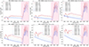 |
Fig. 4. UV band spectra at different Teff and log g. These subplots show the spectra flux under varying Teff (ranging from 3800 K to 12 000 K) and log g (ranging from +1.0 to +6.0), with [Fe/H] changing from metal-rich ([Fe/H] = +1.0) to EMP ([Fe/H] = −4.0). The red curves generally represent higher [Fe/H], while blue curves represent lower [Fe/H]. The transition from red to blue corresponds to the change from high to low [Fe/H], where each curve represents a specific level of [Fe/H]. |
When analysing the UV spectral region within a high-temperature range (9000 K < Teff < 12 000 K), as shown in Fig. 5, we notice some interesting characteristics. Specifically, at higher temperatures, the spectral flux of EMP stars is lower compared to the stars of higher metallicity, with this discrepancy increasing as the temperature rises. Additionally, starting from 3600 Å, the spectral lines show a more concentrated trend (as indicated by the shaded area in Fig. 5), which increases the difficulty of identifying EMP stars at these temperatures.
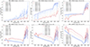 |
Fig. 5. UV band spectra at high Teff. These subplots show the UV spectral flux at various high Teff conditions (ranging from 9000 K to 12 000 K), with a constant log g (e.g. log g = 3.0) and varying [Fe/H] (ranging from +1.0 to −4.0). |
In the mid-to-low temperature range (3700 K < Teff < 7600 K), as illustrated in Fig. 6, the EMP stars tend to show a higher flux level compared to the stars of higher metallicity. As shown in Fig. 7, the impact of different surface gravities indicates that as log g increases, the difference in flux between the metal-poor stars and the stars of higher metallicity decreases, and the spectral-line features become more concentrated. This could similarly present challenges in identifying EMP stars.
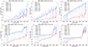 |
Fig. 6. UV band spectra at mid-to-low Teff. These subplots show the UV spectral flux under various mid-to-low Teff (from 3700 K to 7200 K) and a constant log g (e.g. log g = 3.0), with varying [Fe/H] (ranging from +1.0 to −4.0). |
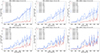 |
Fig. 7. UV band spectra with varying log g. These subplots display the UV spectral flux at a fixed Teff (e.g. Teff = 4200 K), with varying log g (ranging from +1.0 to +6.0) and different [Fe/H] (ranging from +1.0 to −4.0). |
Furthermore, under all physical conditions, minor variations in metallicity lead to a densification of spectral lines. This densification, when coupled with noise, could cause oscillations in the regression results around the actual values, making the regression analysis more sensitive to noise. Therefore, it is crucial to evaluate the classification results at different levels of noise. In Sect. 4.3, we focus on how UV band spectra affect model performance under various noise conditions, especially in identifying EMP stars.
4.3. Noise experiments
Before conducting noise experiments, we first tested our ability to identify EMP stars using spectral data – with and without the inclusion of the UV band spectra – under ideal, noise-free conditions. The results show near-perfect classification accuracy, aligning with our expectations and validating the effectiveness of our model and theoretical spectra. We then analysed the impact of different S/N levels (S/N = 10, 20, 30) on our capability to search for EMP stars using the same approach.
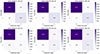 |
Fig. 8. Confusion matrices for identifying EMP stars at different S/N levels. The top panels show the results with UV band spectra at S/N of 10, 20, and 30, while the bottom panels show them without UV band spectra. In each matrix, the upper left and lower right corners show the counts of correctly classified normal stars (label 0) and EMP stars (label 1), respectively. The lower left corner indicates the number of normal stars mistakenly classified as EMP stars (false positives), and the upper right corner represents EMP stars incorrectly identified as normal stars (false negatives). The intensity of the colour indicates the quantity, with darker colours representing higher numbers and lighter colours indicating lower numbers. |
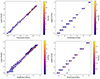 |
Fig. 9. Prediction results for [Fe/H] and [C/Fe] with and without the UV band spectra (ranging from 2550–10 000 Å and 4000–10 000 Å, respectively). The top panels compare the predicted and actual values of [Fe/H] and [C/Fe] when the UV band spectra are included. The bottom panels show the prediction results without the UV band spectra. |
As illustrated in Fig. 8, the model that includes UV band spectra shows a distinct advantage in identifying true EMP stars (labelled 1), even at a lower S/N of 10. Specifically, this model correctly identified the majority of EMP stars, with only 59 true EMP stars misclassified. In contrast, the model that does not include UV band spectra failed to recognise 465 EMP stars. When the S/N increases to 20, the model including the UV band spectra still shows a strong capability in identifying EMP stars, misclassifying only 44 EMP stars, while the model without UV band spectra fails to recognise 245 EMP stars. At even higher S/N levels, both models improve in their ability to identifying EMP stars. However, the model with UV band spectra still performs better, with only 13 misclassified EMP stars, compared to 146 unrecognised by the model without UV band spectra.
Table 2 shows that the model with UV band spectra consistently performs better than the model without them – particularly at a low S/N of 10 – in terms of accuracy, recall, and F1 score. Here, recall is a critical metric (measuring the ability of the model to correctly identify positive classes, in this case, EMP stars), because in astrophysical research, missing any EMP star could mean losing valuable information for studying the early Universe. As shown in Table 2, at S/N = 10, the recall for the model including the UV band spectra is 0.94, compared to just 0.48 for the model without the UV band spectra. This indicates that the model that includes UV band spectra is nearly twice as effective at identifying EMP stars under low S/N conditions as the model without. When the S/N increases to 20, the recall of the model with the UV band data remains higher than that of the model without the UV band spectra (0.75 vs. 0.95). At an S/N of 30, the difference in recall between the two models, although smaller (0.95 vs. 0.84), still demonstrates the superiority of the model with UV band data. Given the limited resources in practical applications, such high recall can maximise the identification of all possible EMP star candidates, greatly reducing the omission of potentially interesting celestial bodies. Under low S/N, the advantage of the model including the UV band data in identifying EMP star candidates is particularly evident. Ultimately, we can conclude that UV band spectra are crucial for improving the identification of EMP stars, especially in low S/N environments.
Performance evaluation metrics for identifying EMP stars at different S/N.
Statistical comparison of prediction errors for [Fe/H] and [C/Fe].
Performance evaluation metrics for identifying CE-EMP stars at different S/N.
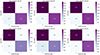 |
Fig. 10. Confusion matrices for identifying CE-EMP stars at different S/N levels. The top panels show the results with UV band spectra at S/N of 10, 20, and 30, while the bottom panels show them without UV band spectra. In each matrix, the upper left and lower right corners show the counts of correctly classified CN-EMP stars (label 0) and CE-EMP stars (label 1), respectively. The lower left corner indicates the number of CN-EMP stars mistakenly classified as CE-EMP stars (false positives), and the upper right corner represents CE-EMP stars incorrectly identified as CN-EMP stars (false negatives). |
4.4. Evaluating [C/Fe]
Based on the experiments and analyses in Sects. 4.1 and 4.3, we quantitatively evaluated the contribution of UV band spectra in estimating [Fe/H] and [α/Fe] using the SPT model. Additionally, we tested the impact of these spectral data on identifying EMP stars at various noise levels. In this section, we continue to use the SPT model to estimate [C/Fe] based on the second set of synthesised spectra from Sect. 2.3 to better distinguish between CE-EMP stars and CN-EMP stars. As shown in the Table 3, the model including UV band spectra achieved reductions in MAE and σ by 0.03 and 0.04, respectively. Furthermore, Fig. 9 shows that the predictions using UV band spectra are more closely aligned with the actual values, indicating reduced uncertainty.
We also analysed the impact of UV band spectra on the identification of CE-EMP stars at different noise levels. Table 4 shows that the model with UV band spectra outperformed the model without them in terms of accuracy, recall, and F1 score. Figure 10 clearly shows that, across three different noise levels, the model including UV band spectra identified an additional 268, 340, and 101 CE-EMP stars, respectively, compared to the model without UV data.
These indicate that the inclusion of UV band spectra enhances the effectiveness of CE-EMP star identification. This improvement is especially noticeable in high-noise environments, where the model represents better performance.
5. Conclusion
In this study, we quantitatively evaluated the contribution of UV band spectra in predicting [Fe/H], [α/Fe], and [C/Fe] using the SPT model. Additionally, we analysed the differences in [Fe/H] spectral lines under different physical conditions and tested the impact of UV band spectra on our ability to identify EMP and CE-EMP stars at different noise levels.
Our results show that the inclusion of UV band spectra reduces the MAE for [Fe/H], [α/Fe], and [C/Fe] by 0.04, 0.04, and 0.03, respectively, with reductions in σ of 0.02, 0.03, and 0.04. Further spectral analysis reveals unique spectral-line features of EMP stars at different effective temperatures and surface gravity conditions, particularly in the UV band, which is useful for identifying EMP stars. We observe that at higher effective temperatures (9000 K < Teff < 12 000 K), metal-poor stars show lower spectral flux compared to normal stars, and this difference increases with rising effective temperature. Conversely, in the mid-to-low effective temperature range (3700 K < Teff < 7600 K), metal-poor stars tend to show relatively higher flux levels.
In our noise experiments, we find that UV band spectra significantly boost our ability to identify EMP and CE-EMP stars in low-S/N conditions. We tested different S/N levels (S/N = 10, 20, 30) and observe that models including UV band spectra show an advantage in identifying true EMP and CE-EMP stars. As S/N increases, these models maintain high recall, demonstrating robustness across a range of S/N environments. Compared to models without UV band spectra, these models effectively reduce the risk of missing potentially interesting stellar candidates, ensuring a more comprehensive identification of all possible EMP and CE-EMP star candidates.
In summary, this study reveals the importance of UV spectral data in improving the identification of EMP and CE-EMP stars in future astrophysical observations, particularly for projects like the CSST.
Acknowledgments
We thank the anonymous referee for useful comments that helped us improve the manuscript substantially. This work is supported by the National Natural Science Foundation of China (NSFC) under grant No. 12090044 and 11873037, the science research grants from the China Manned Space Project with No. CMS-CSST-2021-B05 and CMS-CSST-2021-A08, the Natural Science Foundation of Shandong Province under grant No. ZR2022MA076, and partially supported by the Young Scholars Program of Shandong University, Weihai (2016WHWLJH09) and GHfund A (202202018107). X.K is supported by the National Natural Science Foundation of China under grant No. 11803016. Z.Y is supported by the Shandong Province Natural Science Foundation grant No. ZR2022MA089.
References
- Beers, T. C., & Christlieb, N. 2005, ARA&A, 43, 531 [NASA ADS] [CrossRef] [Google Scholar]
- Belokurov, V., & Kravtsov, A. 2022, MNRAS, 514, 689 [NASA ADS] [CrossRef] [Google Scholar]
- Bonifacio, P., Caffau, E., & Spite, M. 2019, BAAS, 51, 546 [NASA ADS] [Google Scholar]
- Buder, S., Asplund, M., Duong, L., et al. 2018, MNRAS, 478, 4513 [Google Scholar]
- Cao, Y., Gong, Y., Meng, X.-M., et al. 2018, MNRAS, 480, 2178 [Google Scholar]
- Castelli, F., & Kurucz, R. L. 2003, in Modelling of Stellar Atmospheres, eds. N. Piskunov, W. W. Weiss, & D. F. Gray, 210, A20 [Google Scholar]
- Chiti, A., Frebel, A., Mardini, M. K., et al. 2021, ApJS, 254, 31 [NASA ADS] [CrossRef] [Google Scholar]
- Conroy, C., Weinberg, D. H., Naidu, R. P., et al. 2022, OJAp, submitted [arXiv:2204.02989] [Google Scholar]
- Da Costa, G. S., Bessell, M. S., Nordlander, T., et al. 2023, MNRAS, 520, 917 [NASA ADS] [CrossRef] [Google Scholar]
- Das, P., Hawkins, K., & Jofré, P. 2020, MNRAS, 493, 5195 [NASA ADS] [CrossRef] [Google Scholar]
- Deng, L.-C., Newberg, H. J., Liu, C., et al. 2012, Res. Astron. Astrophys., 12, 735 [Google Scholar]
- El-Badry, K., Bland-Hawthorn, J., Wetzel, A., et al. 2018, MNRAS, 480, 652 [NASA ADS] [CrossRef] [Google Scholar]
- Frebel, A., & Norris, J. E. 2015, ARA&A, 53, 631 [NASA ADS] [CrossRef] [Google Scholar]
- Gilmore, G., Randich, S., Worley, C. C., et al. 2022, A&A, 666, A120 [NASA ADS] [CrossRef] [EDP Sciences] [Google Scholar]
- Gong, Y., Liu, X., Cao, Y., et al. 2019, ApJ, 883, 203 [NASA ADS] [CrossRef] [Google Scholar]
- Gray, R. O., & Corbally, C. J. 1994, AJ, 107, 742 [Google Scholar]
- Hawkins, K., Jofré, P., Masseron, T., & Gilmore, G. 2015, MNRAS, 453, 758 [NASA ADS] [CrossRef] [Google Scholar]
- Heger, A., & Woosley, S. E. 2010, ApJ, 724, 341 [Google Scholar]
- Helmi, A. 2020, ARA&A, 58, 205 [Google Scholar]
- Horta, D., Schiavon, R. P., Mackereth, J. T., et al. 2021, MNRAS, 500, 1385 [Google Scholar]
- Hughes, A. C. N., Spitler, L. R., Zucker, D. B., et al. 2022, ApJ, 930, 47 [NASA ADS] [CrossRef] [Google Scholar]
- Husser, T. O., Wende-von Berg, S., Dreizler, S., et al. 2013, A&A, 553, A6 [NASA ADS] [CrossRef] [EDP Sciences] [Google Scholar]
- Ishigaki, M. N., Hartwig, T., Tarumi, Y., et al. 2021, MNRAS, 506, 5410 [NASA ADS] [CrossRef] [Google Scholar]
- Jones, S., Côté, B., Röpke, F. K., & Wanajo, S. 2019, ApJ, 882, 170 [NASA ADS] [CrossRef] [Google Scholar]
- Kamann, S., Husser, T. O., Brinchmann, J., et al. 2016, A&A, 588, A149 [NASA ADS] [CrossRef] [EDP Sciences] [Google Scholar]
- Li, H., Tan, K., & Zhao, G. 2018, ApJS, 238, 16 [CrossRef] [Google Scholar]
- Limongi, M., & Chieffi, A. 2012, ApJS, 199, 38 [NASA ADS] [CrossRef] [Google Scholar]
- Liu, X. W., Yuan, H. B., Huo, Z. Y., et al. 2014, in Setting the Scene for Gaia and LAMOST, eds. S. Feltzing, G. Zhao, N. A. Walton, P. Whitelock, 298, 310 [NASA ADS] [Google Scholar]
- Lu, X., Yuan, H., Xu, S., et al. 2024, ApJS, 271, 26 [NASA ADS] [CrossRef] [Google Scholar]
- Lucatello, S., Beers, T. C., Christlieb, N., et al. 2006, ApJ, 652, L37 [NASA ADS] [CrossRef] [Google Scholar]
- Majewski, S. R., Schiavon, R. P., Frinchaboy, P. M., et al. 2017, AJ, 154, 94 [NASA ADS] [CrossRef] [Google Scholar]
- Pang, X., Shu, Q., Wang, L., & Kouwenhoven, M. B. N. 2022, Res. Astron. Astrophys., 22, 095015 [CrossRef] [Google Scholar]
- Placco, V. M., Frebel, A., Beers, T. C., & Stancliffe, R. J. 2014, ApJ, 797, 21 [Google Scholar]
- Placco, V. M., Beers, T. C., Santucci, R. M., et al. 2018, AJ, 155, 256 [Google Scholar]
- Randich, S., Gilmore, G., Magrini, L., et al. 2022, A&A, 666, A121 [NASA ADS] [CrossRef] [EDP Sciences] [Google Scholar]
- Rix, H.-W., Chandra, V., Andrae, R., et al. 2022, ApJ, 941, 45 [NASA ADS] [CrossRef] [Google Scholar]
- Rockosi, C. M., Lee, Y. S., Morrison, H. L., et al. 2022, ApJS, 259, 60 [CrossRef] [Google Scholar]
- Sneden, C., Boesgaard, A. M., Cowan, J. J., et al. 2023, ApJ, 953, 31 [CrossRef] [Google Scholar]
- Starkenburg, E., Oman, K. A., Navarro, J. F., et al. 2017, MNRAS, 465, 2212 [NASA ADS] [CrossRef] [Google Scholar]
- Steinmetz, M., Zwitter, T., Siebert, A., et al. 2006, AJ, 132, 1645 [Google Scholar]
- Wanajo, S. 2018, ApJ, 868, 65 [CrossRef] [Google Scholar]
- Wang, R., & Luo, A. 2019, ASP Conf. Ser., 523, 119 [NASA ADS] [Google Scholar]
- Yanny, B., Rockosi, C., Newberg, H. J., et al. 2009, AJ, 137, 4377 [Google Scholar]
- Yoon, J., Beers, T. C., Dietz, S., et al. 2018, ApJ, 861, 146 [NASA ADS] [CrossRef] [Google Scholar]
- York, D. G., Adelman, J., Anderson, J. E., Jr., et al. 2000, AJ, 120, 1579 [NASA ADS] [CrossRef] [Google Scholar]
- Zhan, H. 2011, Sci. Sin. Phys. Mech. Astron., 41, 1441 [NASA ADS] [CrossRef] [Google Scholar]
- Zhang, M., Wu, F., Bu, Y., et al. 2024a, A&A, 683, A163 [NASA ADS] [CrossRef] [EDP Sciences] [Google Scholar]
- Zhang, J., Tang, B., Chang, J., et al. 2024b, Res. Astron. Astrophys., 24, 015011 [CrossRef] [Google Scholar]
All Tables
All Figures
|
Fig. 1. Comparative spectral profiles pre- and post-resolution reduction for a stellar model with Teff = 3500 K, log g = +4.0, and [α/Fe]= + 3.0. The grey curve depicts the original high-resolution spectrum. The red curve illustrates the spectrum after Gaussian convolution processing, which reduces the resolution to simulate the observational effect of the CSST. The wavelength range extends from 2550 to 10 000 Å, displaying the changes from the UV to the NIR region following the resolution-degradation process. |
| In the text | |
|
Fig. 2. Model architecture. At its core, the architecture comprises an embedded input layer and an SPT backbone, which together form the fundamental feature-extraction module. Building on this, the model bifurcates into two specialised branches: a regression head tasked with the precise prediction of stellar [Fe/H] and [α/Fe] indices, and a classification head designed for the binary classification of EMP and non-EMP stars. |
| In the text | |
|
Fig. 3. Prediction results for [Fe/H] and [α/Fe] with and without the UV band spectra (ranging from 2550–10 000 Å and 4000–10 000 Å, respectively). The top panels compare the predicted and actual values of [Fe/H] and [α/Fe] when the UV band spectra are included. The colour intensity represents the density of data points, ranging from blue (low density) to red (high density). The dashed lines represent the identity line. The bottom panels show the prediction results without the UV band spectra. |
| In the text | |
|
Fig. 4. UV band spectra at different Teff and log g. These subplots show the spectra flux under varying Teff (ranging from 3800 K to 12 000 K) and log g (ranging from +1.0 to +6.0), with [Fe/H] changing from metal-rich ([Fe/H] = +1.0) to EMP ([Fe/H] = −4.0). The red curves generally represent higher [Fe/H], while blue curves represent lower [Fe/H]. The transition from red to blue corresponds to the change from high to low [Fe/H], where each curve represents a specific level of [Fe/H]. |
| In the text | |
|
Fig. 5. UV band spectra at high Teff. These subplots show the UV spectral flux at various high Teff conditions (ranging from 9000 K to 12 000 K), with a constant log g (e.g. log g = 3.0) and varying [Fe/H] (ranging from +1.0 to −4.0). |
| In the text | |
|
Fig. 6. UV band spectra at mid-to-low Teff. These subplots show the UV spectral flux under various mid-to-low Teff (from 3700 K to 7200 K) and a constant log g (e.g. log g = 3.0), with varying [Fe/H] (ranging from +1.0 to −4.0). |
| In the text | |
|
Fig. 7. UV band spectra with varying log g. These subplots display the UV spectral flux at a fixed Teff (e.g. Teff = 4200 K), with varying log g (ranging from +1.0 to +6.0) and different [Fe/H] (ranging from +1.0 to −4.0). |
| In the text | |
|
Fig. 8. Confusion matrices for identifying EMP stars at different S/N levels. The top panels show the results with UV band spectra at S/N of 10, 20, and 30, while the bottom panels show them without UV band spectra. In each matrix, the upper left and lower right corners show the counts of correctly classified normal stars (label 0) and EMP stars (label 1), respectively. The lower left corner indicates the number of normal stars mistakenly classified as EMP stars (false positives), and the upper right corner represents EMP stars incorrectly identified as normal stars (false negatives). The intensity of the colour indicates the quantity, with darker colours representing higher numbers and lighter colours indicating lower numbers. |
| In the text | |
|
Fig. 9. Prediction results for [Fe/H] and [C/Fe] with and without the UV band spectra (ranging from 2550–10 000 Å and 4000–10 000 Å, respectively). The top panels compare the predicted and actual values of [Fe/H] and [C/Fe] when the UV band spectra are included. The bottom panels show the prediction results without the UV band spectra. |
| In the text | |
|
Fig. 10. Confusion matrices for identifying CE-EMP stars at different S/N levels. The top panels show the results with UV band spectra at S/N of 10, 20, and 30, while the bottom panels show them without UV band spectra. In each matrix, the upper left and lower right corners show the counts of correctly classified CN-EMP stars (label 0) and CE-EMP stars (label 1), respectively. The lower left corner indicates the number of CN-EMP stars mistakenly classified as CE-EMP stars (false positives), and the upper right corner represents CE-EMP stars incorrectly identified as CN-EMP stars (false negatives). |
| In the text | |
Current usage metrics show cumulative count of Article Views (full-text article views including HTML views, PDF and ePub downloads, according to the available data) and Abstracts Views on Vision4Press platform.
Data correspond to usage on the plateform after 2015. The current usage metrics is available 48-96 hours after online publication and is updated daily on week days.
Initial download of the metrics may take a while.