| Issue |
A&A
Volume 689, September 2024
|
|
|---|---|---|
| Article Number | A313 | |
| Number of page(s) | 13 | |
| Section | Galactic structure, stellar clusters and populations | |
| DOI | https://doi.org/10.1051/0004-6361/202450270 | |
| Published online | 20 September 2024 | |
Dynamics of star clusters with tangentially anisotropic velocity distribution
1
Astronomical Institute of the Czech Academy of Sciences, Boční II 1401, 141 00 Prague 4, Czech Republic
2
Department of Astronomy, Indiana University, Swain Hall West, 727 E 3rd Street, Bloomington, IN 47405, USA
3
Aventinum Publishing House, Tolstého 22, 101 00 Prague 10, Czech Republic
4
School of Mathematics and Maxwell Institute for Mathematical Sciences, University of Edinburgh, Kings Buildings, Edinburgh EH9 3FD, UK
5
Institute for Astronomy, University of Edinburgh, Royal Observatory, Blackford Hill, Edinburgh EH9 3HJ, UK
Received:
5
April
2024
Accepted:
29
May
2024
Abstract
Context. Recent high-precision observations with HST and Gaia enabled new investigations of the internal kinematics of star clusters (SCs) and the dependence of kinematic properties on the stellar mass. These studies raised new questions about the dynamical evolution of self-gravitating stellar systems.
Aims. We aim to develop a more complete theoretical understanding of how the various kinematical properties of stars affect the global dynamical development of their host SCs.
Methods. We perform N-body simulations of globular clusters with isotropic, radially anisotropic, and tangentially anisotropic initial velocity distributions. We also study the effect of an external Galactic tidal field.
Results. We obtain three main results. First, compared to the conventional, isotropic case, the relaxation processes are accelerated in the tangentially anisotropic models and, in agreement with our previous investigations, are slower in the radially anisotropic ones. This leads to, for example, more rapid mass segregation in the central regions of the tangential models or their earlier core collapse. Second, although all SCs become isotropic in the inner regions after several relaxation times, we observe differences in the anisotropy profile evolution in the outer cluster regions – all tidally filling models gain tangential anisotropy there, while the underfilling models become radially anisotropic. Third, we observe different rates of evolution towards energy equipartition (EEP). While all SCs evolve towards EEP in their inner regions (regardless of the filling factor), the outer regions of the tangentially anisotropic and isotropic models are evolving to an ‘inverted’ EEP (i.e. with the high-mass stars having higher velocity dispersion than the low-mass ones). The extent (both spatial and temporal) of this inversion can be attributed to the initial velocity anisotropy – it grows with increasing tangential anisotropy and decreases as the radial anisotropy rises.
Key words: methods: numerical / stars: kinematics and dynamics / globular clusters: general
Corresponding author; This email address is being protected from spambots. You need JavaScript enabled to view it. .
© The Authors 2024
 Open Access article, published by EDP Sciences, under the terms of the Creative Commons Attribution License (https://creativecommons.org/licenses/by/4.0), which permits unrestricted use, distribution, and reproduction in any medium, provided the original work is properly cited.
This article is published in open access under the Subscribe to Open model. This email address is being protected from spambots. You need JavaScript enabled to view it. to support open access publication.
1. Introduction
Recent observations from the Hubble Space Telescope and Gaia along with data from large spectroscopic surveys have provided many new insights into the internal kinematical properties of star clusters (SCs; see e.g. Bellini et al. 2014, 2017, 2018; Watkins et al. 2015; Ferraro et al. 2018; Libralato et al. 2018; Bianchini et al. 2018; Kamann et al. 2018; Jindal et al. 2019; Cohen et al. 2021; Vasiliev & Baumgardt 2021). Complementary studies show that the initial velocity distribution of a SC has a significant effect on its dynamical evolution (e.g. Einsel & Spurzem 1999; Kim et al. 2002; Bianchini et al. 2016, 2017; Aros et al. 2020; Livernois et al. 2022, 2023), and that kinematical signatures also provide a useful way to characterise the formation history of SCs or the ‘multiple stellar population’ conundrum, which remains a focus of current research (e.g. Bellini et al. 2015; Libralato et al. 2019; Cordoni et al. 2020; Vesperini et al. 2021). All these findings have highlighted the need for an improved theoretical understanding of SCs, and the recent observational results of Watkins et al. (2022) further show the importance of studying the different kinematical properties of these stellar systems.
The phenomenological motivation for exploring more complex initial conditions, particularly in the velocity space, is to assess the impact and survivability of any primordial kinematic signatures; ideally, in order to distinguish them from evolutionary ones. Therefore, here we present the fourth paper in a series where we investigate the dynamical processes taking place during the evolution of SCs, with a specific focus on the consequences regarding their stellar kinematics. In Pavlík & Vesperini (2021, hereafter PV1), we provided novel insights into the evolution of SCs towards energy equipartition (EEP) using models with isotropic and radially anisotropic velocity distributions. In Pavlík & Vesperini (2022a, hereafter PV2), we focused on the strength of the galactic tidal field and the observable parameters to facilitate verification of our results with observations. In Pavlík & Vesperini (2022b, hereafter PV3), we further studied the properties of binary stars and mass segregation in the isotropic and radially anisotropic SCs1.
In the present paper, we venture to the other end of the kinematical spectrum, the lesser-known territory of tangential anisotropy. Anisotropy in the tangential direction has gained some attention in conjunction with equilibrium modelling efforts of stellar systems with a central black hole (see e.g. Cohn & Kulsrud 1978; Young 1980; Goodman & Binney 1984; Feldmeier-Krause et al. 2017; Zhang & Amaro Seoane 2024)2. In addition, tangential anisotropy was reported to appear in the outskirts of evolved, tidally limited SCs as a result of stellar escape (Tiongco et al. 2016), and was briefly discussed in the context of long-term evolution of SCs by Breen et al. (2017) and Rozier et al. (2019). Recently, Lahén et al. (2020) gave it some renewed attention after finding signatures of tangential anisotropy in the simulations of low-mass young SCs; however, this kinematical regime still remains understudied. Our aim now is to provide further insights into the relaxation processes in tangentially anisotropic SCs and to expand the very few previous works on this topic.
2. Methods
We simulated N-body models with N0 = 105 stars, an initial King (1966) profile of W0 = 6, and stellar masses drawn from the Kroupa (2001) initial mass function (IMF) within 0.1 ≤ m/M⊙ ≤ 1.0. All models were integrated in NBODY6++GPU (Wang et al. 2015). There were no primordial binary stars but the dynamical formation of binaries was permitted in the simulations (in the following analyses, those are replaced by their centres of mass). The modelled clusters were placed on a circular orbit in a Keplerian Galactic potential with two different filling factors; that is, the initial ratio of the tidal radius, rt, to the King model truncation radius, rK, was either equal to one or ten. We note that all radii in this work are calculated with respect to the cluster’s density centre, as provided by NBODY6++GPU (see also Casertano & Hut 1985; Aarseth 2003).
We considered four sets of initial conditions based on the velocity anisotropy profile. Two of those models – the isotropic one (iso-u/f) and the one with isotropic distribution of velocities in the core but gradual radial anisotropy (rh1-u/f) – were analysed in PV1 and PV2, and are included here to allow for a more direct and detailed comparison. The remaining two models (labelled rad-u/f and tan-u/f) started with a fully radial or fully tangential constant level of anisotropy, respectively. The initial velocity distributions were set up numerically with AGAMA using the Cuddeford–Osipkov–Merritt profile (Osipkov 1979; Merritt 1985; Cuddeford 1991; Vasiliev 2019):
 (1)
(1)
where σrad and σtan are the radial and tangential stellar velocity dispersions, respectively. The anisotropy radius, ra, determines how steeply the profile grows towards radial anisotropy. The specific values for each model are listed in Table 1 and the initial radial profiles of β(r) are plotted in Fig. 1. We note that the filling and underfilling models start with the same anisotropy profiles, and therefore the only difference between the two is the size of the tidal radius.
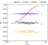 |
Fig. 1. Initial velocity anisotropy profiles of the models. See also Eq. (1) and Table 1. The radial distance is shown in terms of the initial half-mass radius, with each point corresponding to an increment of 2% of mass in the initial Lagrangian radii of the SC. |
Parameters of the models.
Despite their kinematical differences, all models have the same initial spatial structure and half-mass radius, and thus the initial half-mass relaxation time for all of them is given by
 (2)
(2)
in Hénon units (see e.g. Heggie & Mathieu 1986; Heggie & Hut 2003; Heggie 2014). However, this definition does not take into account the initial velocity distributions, which are responsible for different stellar orbits in the SCs and consequently for the variation in the rate of mass loss, the rate of the mixing of stars, and the rate of mass segregation. All this leads to differences in the timescales of the relaxation processes (the same effect has also been noted by Breen et al. 2017; PV1; PV2,PV3).
We can see a manifestation of this when we plot the initial relaxation time as a function of radius,
 (3)
(3)
in Hénon units (see Heggie & Hut 2003; Binney & Tremaine 2008; Merritt 2013). Here Λ = 0.02 N0, consistently with Eq. (2), ⟨m(r)⟩ is the mean mass of stars up to the radius r, ρ(r) is their density, and σ(r) is their velocity dispersion. Figure 2 shows that the relaxation time in the core is two to three times lower in the tangentially anisotropic model than in the other models and this difference is present up to approximately two half-mass radii.
3. Results: Underfilling models
We note that some of the following figures contain both filling and underfilling models for easier visual comparison. Nevertheless, to help us isolate the internal dynamical effects from those related to the external tidal field, we first focus on the underfilling SCs and compare the filling and underfilling SCs in Sect. 4.
3.1. Structural evolution
As illustrated in the top row of plots in Fig. 3, for the underfilling SCs, the tangential model (tan-u) shows the slowest expansion (see the solid black lines for the 99% Lagrangian radius; hereafter L.r.) and the fastest evolution towards core collapse (see the green line representing the core radius). This is then followed by iso-u, rad-u, and rh1-u (with the latter exhibiting core collapse more than 2 trh, 0 later than tan-u). Both dynamical effects (i.e. the rates of expansion and collapse) are caused by the fractions of tangentially and radially moving stars in the SCs. A larger fraction of stars move within circular shells in the tangentially anisotropic cluster, whereas the radially anisotropic SCs are initialised with a larger number of very eccentric orbits. First, this helps the radially anisotropic SCs to expand more rapidly. Second, stars on radial orbits contribute to heating up the cluster core, delaying its core collapse (see PV1 and PV2 for further discussion). In the tangentially anisotropic model, on the other hand, the smaller fraction of radially orbiting stars implies that this heat source is reduced. Consequently, the centre of tan-u has a smaller central velocity dispersion than the other models and the central relaxation time is shorter (see also Fig. 2).
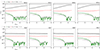 |
Fig. 3. Time evolution of the radial structure of the underfilling SCs (top row) and the filling SCs (bottom row). We show the core radius (as calculated by NBODY6++GPU), the 1% and 99% L.r., the half-mass radius, and the tidal radius (see also the legend). |
3.2. Mass loss and mass segregation
An important factor affecting the dynamical evolution of the studied systems is mass loss, which we visualise in the left-hand panel of Fig. 4 using the total mass of each SC throughout its evolution. We note that the underfilling models lost up to 5% of their initial mass by the end of the simulation – in particular, tan-u lost slightly less mass over time than iso-u and a few per cent less than both radially anisotropic SCs. While these numbers are small, they are not negligible when compared to the total mass loss. These differences are a consequence of anisotropy and the number of stars on very elongated eccentric orbits, which are more likely to escape.
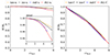 |
Fig. 4. Total mass of the underfilling (left) and filling models (right) at time t, shown as a fraction of the initial SC mass, M0. |
The left-hand panel of Fig. 5 includes the evolution of the mean stellar mass. We note a clear signature of core collapse as the first spike on each curve. Due to the relaxation processes before core collapse, the low-mass stars typically evaporate from the SC at a higher rate than the higher-mass stars (which in turn sink inwards) and the overall ⟨m⟩ should increase. We further illustrate this expansion of the low-mass population with the dotted lines in the top row of Fig. 6. The radial profiles of low-mass stars are very similar in all underfilling models up to 75% L.r. and only differ at higher radii due to a more anisotropy-driven cluster expansion. Immediately after core collapse, the mean mass is expected to drop down due to the additional ejection of massive stars and hard binaries undergoing close interactions in the central regions, which explains the spike in the left-hand panel of Fig. 5 (see e.g. also Aarseth 1972; Fujii & Portegies Zwart 2014; Pavlík & Šubr 2018).
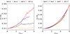 |
Fig. 5. Mean stellar mass in solar masses at time t in the underfilling (left) and filling models (right). The vertical axes have different scales. |
In our case, the left-hand panel of Fig. 5 further reveals that both radially anisotropic models (rad-u and rh1-u) exhibit the highest increase in mean mass and this growth continues even after core collapse. This is due to the higher rate of evaporation of stars on extremely eccentric orbits. On the other hand, the mean mass in the tangentially anisotropic SC (tan-u) remains almost constant even before core collapse, which is mainly caused by the very low initial mass loss (again, see the yellow dashed line in the left-hand panel of Fig. 4). Unlike the radial models, iso-u and tan-u also show almost no evolution of ⟨m⟩ in the post-core-collapse phase.
Regarding mass segregation, PV3 previously concluded that it proceeds at different rates in the outer and inner regions of isotropic and radially anisotropic SCs. The models in PV3 are similar to our iso-u and rh1-u but contain 10 % primordial binaries, which we have not included in the simulations presented in this paper. Nonetheless, the same conclusion can be drawn from our models. Specifically, in the top row of Fig. 6, the lowermost solid line representing the 1% L.r. of the massive stars has slower contraction in both radially anisotropic models than in the isotropic or tangentially anisotropic models. On the contrary, the uppermost solid line, which shows the 90% L.r., significantly decreases in both radial models (rh1-u and rad-u), only slowly decreases in iso-u, but stays constant in the tangentially anisotropic model (see the top-left panel of Fig. 6).
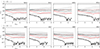 |
Fig. 6. Time evolution of the Lagrangian radii of two stellar mass groups: low-mass (‘L’, m ≤ 0.2 M⊙, dotted lines) and high-mass (‘H’, m ≥ 0.9 M⊙, solid lines). The curves represent 1, 50, 75, and 90% of the total mass of the corresponding mass group (from bottom to top; the half-mass radius is also highlighted in red). The cluster tidal radius is the top dashed line. |
We further investigate the rate of mass segregation by adopting the parameter introduced by Gill et al. (2008) in the left-hand panel of Fig. 7, where we compare the mean stellar masses in three regions, pairwise: namely the core (0–5% L.r.), around the half-mass radius (45–50% L.r.), and the outer regions (70–75% L.r.). There is a clear indication that, before core collapse, tan-u experiences the slowest mass segregation in the outer regions of all the models (see how the yellow circles are below the other circles). However, tan-u initially shows somewhat more rapid mass segregation than the other models in the inner regions (see the yellow crosses on top of all the datasets). As discussed in PV3, the speeding up of mass segregation in the outer regions of the anisotropic model (relative to the segregation rate in the isotropic model) is caused by the enhanced rate of migration of the massive stars on radial orbits, and the delay in mass segregation in the core of the same model is due to the heating up by the larger number of stars on eccentric orbits. We can extrapolate the arguments proposed in PV3 to the models in our work. Specifically, the tangentially anisotropic model (tan-u), which has very few of these elongated orbits, has the shortest relaxation time in the core and the fastest mass segregation there. The other models are then almost ordered in the left-hand panel of Fig. 7 by the amount of initial radial anisotropy (we note that although rad-u has a constant level of radial anisotropy at all r, rh1-u reaches higher values of β in the outer regions, which makes it more radially anisotropic in this sense).
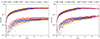 |
Fig. 7. Evolution of mass segregation in the SCs. We compare the mean mass in the core and around the half-mass radius (crosses), and around the half-mass radius and in the outer regions (circles). The ranges of Lagrangian radii from which the mean mass is taken are specified as mass percentages in the labels. The underfilling models are shown in the left-hand panel, and the filling ones in the right-hand panel. |
3.3. Anisotropy evolution
In this section, we present a more detailed exploration of the internal kinematics in the underfilling models. Starting from the initial β(r) profile displayed in Fig. 1, here we plot its temporal evolution in Fig. 8 (see also Appendix A for technical details on how these plots were made). To explore the possible dependence of anisotropy on the stellar mass, in addition to the overall β(r) profile (in the top row of Fig. 8), we also show the anisotropy evolution in three distinct mass groups (as labelled in each of the lower rows of the figure). Two major global features are apparent in the top row of Fig. 8 for all models. First, the regions below the half-mass radius (which is represented by the solid black middle line in each plot) are mostly isotropic (plotted with white) – since the relaxation time decreases by one to two orders of magnitude towards the SC core (as visualised in Fig. 2), the initial anisotropy of the velocity distribution can be quickly removed. Second, the outer regions have significant radial anisotropy (see the red area in the figure) – this is consistent with the findings of Tiongco et al. (2016) and is due to the ongoing relaxation processes as well as the overall expansion of the SC, which we discuss in Sect. 3.2.
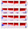 |
Fig. 8. Time evolution of β(r), defined by Eq. (1), in the underfilling models. The top row shows β calculated from the velocity dispersion of all stars in the SC (regardless of mass), and the rows below are calculated for specific mass groups – from the least massive in the second row, intermediate-mass in row three, and the most massive stars in the bottom row (see also the labels on the right-hand side). Red colours correspond to radial anisotropy, and blue colours to tangential anisotropy. If the fit is poorly defined because of an insufficient number of data points in a radius–mass bin, we mask the corresponding pixel in grey. To give a sense of the radial scale and dynamical evolution of the SCs in each plot, we also show the 1% L.r., the half-mass radius, the 99% L.r., and the tidal radius (from bottom to top; black lines). We note that because of the log-scale on the vertical axis, the bins below 2% may appear more prominent than the other bins despite covering a smaller radial range. |
The only model that displays tangential anisotropy is tan-u, which preserves its initial tangential anisotropy imprint during the first 1 − 2 trh, 0 (see the blue region in the top left plot of Fig. 8). However, similarly to the other models, tan-u also becomes isotropic in the inner regions after several relaxation times. A comparison of the blue wedges in the left-most panels in all rows of Fig. 8 further reveals that higher-mass stars in tan-u maintain their tangential anisotropy around and above the half-mass radius for longer than the lower-mass stars. This helps us explain the previously discussed results on the levels of mass segregation (i.e. that it proceeds at the slowest rate in the outer regions of tan-u). If we focus on the other panels in the figure, we also note that no SC develops tangential anisotropy on its own. The only exception is the high-mass population of iso-u, where mild tangential anisotropy appears before core collapse around the half-mass radius (see the faint blue spot around the half-mass radius line in the bottom row of Fig. 8). This is because the massive stars on more radial orbits tend to be mass-segregating into the core, leaving behind the ones on more tangential orbits.
After core collapse, the most massive stars, which segregated to the core, are being ejected from the central region. This dynamical activity causes high fluctuations of β between positive and negative values around 1% L.r., and increases the radial anisotropy in the inner parts of the SCs, which is visible in the bottom row of Fig. 8 as the pale red area just below the half-mass radius. Consistently with our previous discussion regarding the degree of mass segregation, the tangential model shows the smallest increase in β overall, followed by iso-u and then the two radially anisotropic models.
3.4. Energy equipartition
As a SC evolves, the random encounters between stars of different masses guide the system towards EEP (see also, e.g. Spitzer 1969; Inagaki & Wiyanto 1984; Webb & Vesperini 2017). We can quantify the ‘degree’ of EEP with the equipartition mass, meq (a parameter introduced by Bianchini et al. 2016, and extended by PV1 to allow positive and negative values, and formally redefined by Aros & Vesperini 2023):
![Mathematical equation: $$ \begin{aligned} \sigma (r,m) = \left\{ \begin{array}{ll} \sigma _{0} \exp {[-m / (2m_{\rm eq})]}&{, }\,m_{\rm eq} < 0 \\ \sigma _{0} \exp {[-m / (2m_{\rm eq})]}&{, }\,m_{\rm eq} \ge 0 \text{ and} m \le m_{\rm eq} \\ \sigma _{0} e^{-0.5} \sqrt{m_{\rm eq} / m}&{, }\,m_{\rm eq} \ge 0 \text{ and} m > m_{\rm eq} \end{array} \right. \end{aligned} $$](/articles/aa/full_html/2024/09/aa50270-24/aa50270-24-eq4.gif) (4)
(4)
Here, m is the stellar mass and σ0 is a scaling parameter (the velocity dispersion at zero mass). Infinite or very high |meq| shows that there is no relationship between the stellar mass and velocity (i.e. no EEP), whereas if meq decreases below some stellar mass m and meq > 0, particles above that mass achieve EEP. Despite the expectations for evolved systems, some SCs do not reach full EEP (see e.g. Spitzer 1969; Vishniac 1978; Trenti & van der Marel 2013). In PV1, we also found that several SCs develop a trend between velocity dispersion and mass in their outer regions which is opposite to EEP; that is, low-mass stars have systematically lower σ than high-mass stars. Here, we extend these previous results.
In Fig. 9, we plot the evolution of the equipartition mass in the underfilling models. In essence, these plots are similar to those in PV1, PV2, and PV3; however, here we now include two new models and use a much higher radial resolution (compared to only three radial bins in the former works).
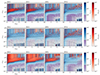 |
Fig. 9. Time evolution of the equipartition mass, meq, in the underfilling SCs (top row – calculated from the 3D velocity dispersion; middle row – calculated only from its radial component; bottom row – calculated only from its tangential component). The regions that evolve towards EEP (to lower positive values of meq) are in shades of blue and purple, and the regions that evolve away from EEP (to negative meq, i.e. away from EEP) are in shades of red; see the colour bars. To give a sense of the radial scale and dynamical evolution of the SCs in each plot, we also show the 1% L.r., half-mass radius, 99% L.r., and the tidal radius (from bottom to top; black lines). If the fit is poorly defined due to an insufficient number of data points in a radius–mass bin, we mask the corresponding pixel with grey. We note that because of the log-scale on the vertical axis, the bins below 2% may appear more prominent than the other bins despite covering a smaller radial range. |
In the top row of Fig. 9, we can see that the SCs evolve towards EEP in the inner regions up to ≲20% L.r. However, only the most massive stars m ≳ 0.5 M⊙ show long-term signs that they achieved EEP (see the purple-coloured bins before and around 2 trh, 0). In certain, very central bins, the lowest value of meq occasionally drops as low as 0.4 M⊙ ± 0.1 M⊙ (the tangential and radial components of σ may give even slightly lower values of meq, but with higher uncertainties), but it never stays this low for more than one time snapshot. The full mass spectrum is therefore never in EEP in our SCs. This behaviour is similar for all the models explored here. On the other hand, the outer regions differ despite having similar levels of anisotropy, as we show in Sect. 3.3. The only underfilling model that has some tendency to evolve towards EEP in the region above the half-mass radius is rh1-u (see the top-right plot in Fig. 9) but meq still fluctuates between positive and negative values (switching between blue and red colours). Thus, we can also draw the conclusion that the system remains in its initial state of velocity equipartition in which the velocity dispersion is independent of the stellar mass (i.e. the slope of σ(m) is almost flat and meq oscillates around ±∞).
The radial component of the velocity dispersion rarely contributes to EEP, as we can see from the scattered purple bins in the middle row of Fig. 9. The tangential component, however, contributes the most to EEP (see the bottom row of Fig. 9). Moreover, in the post-core-collapse evolution of, for example, the rh1-u model, the regions where σtan shows EEP among the high-mass stars extend up to the half-mass radius and the outer regions (see the purple bins in the bottom right panel).
Figure 9 further shows that rad-u, iso-u, and tan-u develop an opposite velocity–mass distribution to what would be expected for a system in partial or full EEP (see the red regions above rh in the top row of the figure). In rad-u and iso-u models, it takes approximately until the moment of core collapse for this trend to disappear; then the outer regions start showing high fluctuations between positive and negative values, as in the case of rh1-u. For the model tan-u, the red region influenced by the negative meq extends up to several relaxation times after core collapse and is also the most extended (reaching down to ≈0.5 rh, initially). In comparison, this region is less extended in the iso-u and rad-u models (see the middle two plots in the top row of Fig. 9).
As illustrated in the bottom two rows of Fig. 9, where we plot meq calculated from the radial and tangential components of σ, respectively, the systematically negative meq (red colour) is clearly visible only in the tangential component. On the other hand, in the radial component, if there is meq < 0, it is rather a fluctuation between positive and negative values (i.e. around meq → ±∞). This is consistent with the discussion in PV2, where it is stated that the inversion of EEP (i.e. the high-mass stars having higher velocity dispersion than the low-mass ones) is mainly apparent in the tangential component of velocity dispersion.
We further corroborate this result with all our models in Fig. 10, where we plot the difference between the velocity dispersion of the high-mass (σH) and the low-mass stars (σL). The top row of plots with the total velocity dispersion shows higher σH than σL in the whole region above the half-mass radius in the models tan-u and iso-u up to core collapse; and similarly in the rad-u model but only in the 70–90% L.r. region. The bottom row of Fig. 10 shows that this observed behaviour is due to the tangential component of σ.
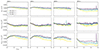 |
Fig. 10. Time evolution of the difference between the velocity dispersion of the high-mass stars (‘H’, 0.8 ≤ m/M⊙ ≤ 1.0) and that of the low-mass stars (‘L’, 0.1 ≤ m/M⊙ ≤ 0.2). The velocity dispersion is scaled by |

The reason behind the observed behaviour of σ and meq in the outer regions is as follows. As briefly mentioned in Sect. 3.3, the more massive stars at large radius may be thought of as two populations: those with more tangential motion (which stay out of the dense central regions, relax slowly, are subject to little mass segregation, and so remain in the outer regions for a long time) and those with more radial motions (which therefore visit the central, dense regions, relax more quickly, are subject to greater mass segregation, and so are removed from the outer regions). Thus, tangential motions of high-mass stars in the outer regions tend to stay higher in tan-u than iso-u or the other models because of the initially lower removal rate of stars with low tangential motions. As discussed in Sect. 3.2, the low-mass stars migrate outwards from the inner regions and their motion is more in the radial direction than the tangential direction. Consequently, this decreases their tangential velocity dispersion in the outer regions (see also PV1 and PV2 for further discussion of the effect of migration of the low-mass stars).
The net result of all this is a positive difference between the velocity dispersion of the high-mass and the low-mass stars in the outer regions (i.e. opposite to what is expected for systems evolving towards EEP). As the relaxation processes in the outer regions become increasingly prominent, σH also starts to decrease and the initial positive difference between σH and σL gradually vanishes (see how the curves representing the different L.r. shells in Fig. 10 become ordered by the mass percentages in all models over time).
Furthermore, the ratio of tangentially to radially moving stars above the half-mass radius seems to directly affect the sign of meq calculated from the tangential component of σ in this region. In other words, the lower the initial value of β, the longer the SC tends to remain in the negative meq regime. The model rh1-u is an extreme case, where the outer region is almost fully radially anisotropic initially (β ≈ 1) and meq (tangential) is almost never negative; although it has the tendency to display negative meq (radial) (compare the plots in the right-hand column of Fig. 9). On the other hand, the model tan-u has β ≈ −0.5 and therefore represents the other extreme, where we see the longest duration of meq < 0 in the outer regions (compare the plots in the left-hand column of Fig. 9). The other two models fit in between these extremes based on their initial β(r) (see the middle two columns of Fig. 9).
4. Results: Filling versus underfilling models
In this section, we discuss the models that started as tidally limited and compare them to their underfilling counterparts.
4.1. Structural evolution
In Sect. 3.1, we point out a trend concerning the order in which the SCs experience core collapse. As Table 1 and the evolution of the L.r. (bottom row of Fig. 3) indicate, this trend seems to be independent of the filling factor. However, since the tidally limited SCs have no room to expand, the stars on the most eccentric orbits with large semi-major axes are being removed more efficiently. Consequently, the role of radial anisotropy in delaying core collapse is reduced and the difference in tcc is not as prominent as in the underfilling models: specifically, iso-f and rad-f are only separated by ≈0.2 trh, 0 (which is within the estimated uncertainties), and the largest span between tan-f and rh1-f is only about 1.4 trh, 0 (compared to ≳2 trh, 0 in the underfilling counterparts).
4.2. Mass loss and mass segregation
We quantify mass loss in the filling models in the right-hand panel of Fig. 4 by plotting the total SC mass in time. We note that while the underfilling SCs only lost a few percent of their mass over the course of several relaxation times, the filling models lost around 50 − 60% by the end of the simulations. The initial slope of the mass-loss curves is also different. There is almost no initial mass loss in the underfilling models but all the filling ones show a short but steep initial decrease in the total mass caused by the primordial escapers. Furthermore, for the underfilling models, there is a change in the rate of mass loss at core collapse (see the break in the slopes of the dashed lines in the inset plot in the left-hand panel of Fig. 4), while for the tidally filling clusters, the mass loss proceeds at almost the same rate, regardless of the initial kinematics or the evolutionary stage. This shows that the tidal limitation plays a much greater role in the overall mass loss than the initial anisotropy in the filling models.
The increased mass loss also affects the evolution of the mean stellar mass, which is plotted in the right-hand panel of Fig. 5; it shows a similar growth in all the filling SCs – with both radially anisotropic SCs increasing only slightly faster (by ≈0.0025 M⊙/trh, 0) than the isotropic or tangentially anisotropic ones. There is also no visible signature of core collapse in the mean stellar mass of the filling models.
Regarding the mass segregation in the filling models, the dotted lines in the bottom row of Fig. 6 show that the radial profiles of the low-mass stars are almost identical throughout the evolution of the SCs (which also agrees with the similarities in the evolution of the mean mass and the rates of mass loss). The Lagrangian radii of the high-mass stars (solid lines in the bottom row of the same figure) follow a qualitatively similar trend as in the underfilling models (top row of the figure). Furthermore, we find similar degrees of mass segregation in the core of both the filling and the underfilling models, but on slightly different timescales (compare the crosses between the right and left-hand panels of Fig. 7). The outer regions (circles in the same figure) also evolve in a similar way; however, because of the high ongoing mass loss in the filling models, its outer ⟨m⟩ is growing even after core collapse.
4.3. Anisotropy evolution
The obvious difference in the evolution of the β(r) profile between the filling (Fig. 11) and underfilling SCs (Fig. 8) is in the outer regions. As the majority of the radially moving stars are removed from the filling clusters, more of those on tangential orbits remain. Consequently, the SCs develop an outer shell with significant tangential anisotropy (see the blue regions around the tidal radius in Fig. 11); this is, again, is consistent with Tiongco et al. (2016). This feature is independent of the stellar mass.
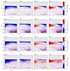 |
Fig. 11. Same as Fig. 8 but for the filling models. The vertical axis has the same range as in Fig. 8 to ease the comparison; we note, however, that the tidal radius limits the SC at a much lower r. |
The regions below the half-mass radius show no qualitative differences between the filling and underfilling SCs before core collapse and only minor deviations can be found after tcc. Specifically, the low-mass stars in the filling models develop more tangential anisotropy in the shell from 0.1 rh, 0 to 1 rh, 0, whereas the high-mass and intermediate-mass stars are slightly less radially anisotropic around the half-mass radius. The whole core region is again noisy, and therefore we do not discuss it here.
4.4. Energy equipartition
We also find similarities when studying the equipartition mass. Apart from the different timescales, the regions up to the half-mass radius appear almost identical in the underfilling models and their filling counterparts (see Figs. 9 and 12, respectively). The only noticeable difference is in the outer regions where, for example, rh1-f does not exhibit the fluctuations we describe in rh1-u, and shows a global evolution towards EEP. Nonetheless, even in the filling SCs, meq stays mostly above 1.0 M⊙ (see the blue regions in Fig. 12) and drops down to ≳0.5 only before core collapse (see the purple regions in the figure) – EEP is never reached in the full mass spectrum. Moreover, in the post-core-collapse evolution, the regions where the high-mass stars show temporary EEP based on our fitting (see Appendix A) are far more scattered throughout the cluster than in the underfilling models, and they are most prominent in the tan-f model.
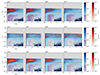 |
Fig. 12. Same as Fig. 9 but for the filling models. The vertical axis has the same range as in Fig. 9 to ease the comparison; we note, however, that the tidal radius limits the SC at a much lower r. |
The outer regions of the models tan-f, iso-f, and rad-f evolve towards an inverted EEP initially, which is characterised by negative values of meq (see the red areas in the top row of Fig. 12). Within several relaxation times, all three models gradually transition back to positive meq and none of them are showing an area dominated by meq < 0 after core collapse. The reason behind the inverted EEP is the same here as in the underfilling SCs – it is driven by the tangential component of σ and depends on the number of massive stars with tangential orbits and the outward migration of the low-mass population. Referring to the discussion in Sect. 3.4, a similar comparison can be made between Fig. 12 (see the extent of the red regions in the bottom row) and Fig. 13, which shows the difference in velocity dispersion between the high-mass and low-mass stars in the filling models.
However, the filling models cannot maintain the negative meq (or the positive difference σH − σL) for the same amount of time as the underfilling models. First, this is due to the tidal limitation, which does not allow the low-mass stars to expand as far as in the underfilling SCs (compare the slopes of the dotted lines in the bottom and top rows of Fig. 6). The second factor is the higher mass-loss rate, which prevents the massive stars from staying within their radial shells for a long period of time, even in the tangentially anisotropic model (see the decreasing trend of all uppermost solid black lines in the bottom row of Fig. 6).
5. Conclusions
We investigated the implications of the initial stellar kinematics for the global dynamical evolution of SCs with 105 stars. We find that the relaxation processes responsible, for example, for mass segregation or EEP, take place over different timescales in the SCs with tangentially anisotropic, isotropic, or radially anisotropic velocity distributions. We also evaluated the effects of the external Galactic tidal field. Our conclusions can be summarised as follows.
The time of core collapse in all SCs depends on the amount of radial velocity anisotropy introduced to the system. In the tidally underfilling SCs, it happens earliest in the tangentially anisotropic model and is delayed by up to ≳2 trh, 0 in the radially anisotropic model (with the isotropic model between the two). The same order is also visible in the tidally filling SCs; however, the time separation of core collapse is not as pronounced because of the higher mass loss, which accelerates the evolution in the radially anisotropic models.
Mass segregation proceeds at different rates in the models. This is consistent with Pavlík & Vesperini (2022b) but here we extend their conclusions by adding the tangentially anisotropic SC. In particular, (i) in the core region, mass segregation is most rapid in the tangentially anisotropic SC and slows down with increasing radial anisotropy; (ii) in the outer regions, mass segregation in the tangentially anisotropic SC is the slowest and accelerates in the models with added radial anisotropy.
All tidally underfilling SCs develop radial anisotropy in their outer regions above the half-mass radius, whereas the filling SCs form a tangentially anisotropic shell below their tidal radii. These results are conststent with Tiongco et al. (2016).
Focusing on the regions below the half-mass radius, all SCs become isotropic there after several relaxation times (we note that this includes even the SC, which started fully tangentially anisotropic). This effect is caused by the much shorter relaxation timescale in the inner regions.
All SCs, regardless of their filling factor, evolve towards EEP in the central regions. The most massive stars there, with m ≳ 0.5 M⊙, are even able to achieve EEP for an extended period of time.
In the outer regions, the evolution differs between the models. The SCs that were initially the most radially anisotropic evolve towards EEP but the other models show an ‘inverted’ evolution in the outer regions, where the high-mass stars tend to have systematically higher velocity dispersion than the low-mass stars. The duration of this inverted EEP increases with the increasing tangential anisotropy in the system, and decreases as the degree of radial anisotropy in the system grows. This result further extends the findings of Pavlík & Vesperini (2021) and Pavlík & Vesperini (2022a).
We note that isotropy and radial and tangential anisotropy in this work always refer to the stellar velocity distributions.
It is important to point out that the models in our study do not have a black hole and tangential anisotropy is considered as primordial.
Acknowledgments
VP has received funding from the European Union’s Horizon Europe and the Central Bohemian Region under the Marie Skłodowska-Curie Actions – COFUND, Grant agreement https://doi.org/10.3030/101081195 (“MERIT”). Views and opinions expressed are, however, those of the authors only and do not necessarily reflect those of the European Union or the Central Bohemian Region. Neither the European Union nor the Central Bohemian Region can be held responsible for them. VP also acknowledges (1) the use of the high-performance storage within his project “Dynamical evolution of star clusters with anisotropic velocity distributions” at Indiana University Bloomington; (2) Lilly Endowment, Inc., through its support for the Indiana University Pervasive Technology Institute; (3) access to computational resources provided by the e-INFRA CZ project (ID:90254), supported by the Ministry of Education, Youth and Sports of the Czech Republic, and (4) the support from the project RVO:67985815 at the Czech Academy of Sciences. ALV acknowledges support from a UKRI Future Leaders Fellowship (MR/S018859/1). For the purpose of Open Access, the authors have applied a Creative Commons Attribution (CC BY) licence to any Author Accepted Manuscript version arising from this submission. The Python programming language with NumPy (Harris et al. 2020) and Matplotlib (Hunter 2007) contributed to this project. This research has made use of NASA’s Astrophysics Data System Bibliographic Services.
References
- Aarseth, S. J. 1972, in Binary Evolution in Stellar Systems, ed. M. Lecar (Netherlands: Springer), 88 [Google Scholar]
- Aarseth, S. J. 2003, Gravitational N-Body Simulations (Cambridge: Cambridge University Press) [Google Scholar]
- Aros, F. I., & Vesperini, E. 2023, MNRAS, 525, 3136 [NASA ADS] [CrossRef] [Google Scholar]
- Aros, F. I., Sippel, A. C., Mastrobuono-Battisti, A., et al. 2020, MNRAS, 499, 4646 [CrossRef] [Google Scholar]
- Bellini, A., Anderson, J., van der Marel, R. P., et al. 2014, ApJ, 797, 115 [Google Scholar]
- Bellini, A., Vesperini, E., Piotto, G., et al. 2015, ApJ, 810, L13 [NASA ADS] [CrossRef] [Google Scholar]
- Bellini, A., Bianchini, P., Varri, A. L., et al. 2017, ApJ, 844, 167 [NASA ADS] [CrossRef] [Google Scholar]
- Bellini, A., Libralato, M., Bedin, L. R., et al. 2018, ApJ, 853, 86 [NASA ADS] [CrossRef] [Google Scholar]
- Bianchini, P., van de Ven, G., Norris, M. A., Schinnerer, E., & Varri, A. L. 2016, MNRAS, 458, 3644 [NASA ADS] [CrossRef] [Google Scholar]
- Bianchini, P., Sills, A., & Miholics, M. 2017, MNRAS, 471, 1181 [Google Scholar]
- Bianchini, P., van der Marel, R. P., del Pino, A., et al. 2018, MNRAS, 481, 2125 [Google Scholar]
- Binney, J., & Tremaine, S. 2008, Galactic Dynamics, 2nd edn. (Princeton: Princeton University Press) [Google Scholar]
- Breen, P. G., Varri, A. L., & Heggie, D. C. 2017, MNRAS, 471, 2778 [NASA ADS] [CrossRef] [Google Scholar]
- Casertano, S., & Hut, P. 1985, ApJ, 298, 80 [Google Scholar]
- Cohen, R. E., Bellini, A., Libralato, M., et al. 2021, AJ, 161, 41 [Google Scholar]
- Cohn, H., & Kulsrud, R. M. 1978, ApJ, 226, 1087 [NASA ADS] [CrossRef] [Google Scholar]
- Cordoni, G., Milone, A. P., Mastrobuono-Battisti, A., et al. 2020, ApJ, 889, 18 [Google Scholar]
- Cuddeford, P. 1991, MNRAS, 253, 414 [NASA ADS] [Google Scholar]
- Einsel, C., & Spurzem, R. 1999, MNRAS, 302, 81 [NASA ADS] [CrossRef] [Google Scholar]
- Feldmeier-Krause, A., Zhu, L., Neumayer, N., et al. 2017, MNRAS, 466, 4040 [NASA ADS] [Google Scholar]
- Ferraro, F. R., Mucciarelli, A., Lanzoni, B., et al. 2018, ApJ, 860, 50 [NASA ADS] [CrossRef] [Google Scholar]
- Fujii, M. S., & Portegies Zwart, S. 2014, MNRAS, 439, 1003 [NASA ADS] [CrossRef] [Google Scholar]
- Gill, M., Trenti, M., Miller, M. C., et al. 2008, ApJ, 686, 303 [CrossRef] [Google Scholar]
- Goodman, J., & Binney, J. 1984, MNRAS, 207, 511 [NASA ADS] [CrossRef] [Google Scholar]
- Harris, C. R., Millman, K. J., van der Walt, S. J., et al. 2020, Nature, 585, 357 [NASA ADS] [CrossRef] [Google Scholar]
- Heggie, D. C. 2014, ArXiv e-prints [arXiv:1411.4936v2] [Google Scholar]
- Heggie, D. C., & Hut, P. 2003, The Gravitational Million-Body Problem: A Multidisciplinary Approach to Star Cluster Dynamics (Cambridge: Cambridge University Press) [Google Scholar]
- Heggie, D. C., & Mathieu, R. D. 1986, in The Use of Supercomputers in Stellar Dynamics, eds. P. Hut, & S. L. W. McMillan (Berlin, Heidelberg: Springer), 233 [NASA ADS] [CrossRef] [Google Scholar]
- Hunter, J. D. 2007, Comput. Sci. Eng., 9, 90 [NASA ADS] [CrossRef] [Google Scholar]
- Inagaki, S., & Wiyanto, P. 1984, PASJ, 36, 391 [NASA ADS] [Google Scholar]
- Jindal, A., Webb, J. J., & Bovy, J. 2019, MNRAS, 487, 3693 [Google Scholar]
- Kamann, S., Husser, T. O., Dreizler, S., et al. 2018, MNRAS, 473, 5591 [NASA ADS] [CrossRef] [Google Scholar]
- Kim, E., Einsel, C., Lee, H. M., Spurzem, R., & Lee, M. G. 2002, MNRAS, 334, 310 [NASA ADS] [CrossRef] [Google Scholar]
- King, I. R. 1966, AJ, 71, 64 [Google Scholar]
- Kroupa, P. 2001, MNRAS, 322, 231 [NASA ADS] [CrossRef] [Google Scholar]
- Lahén, N., Naab, T., Johansson, P. H., et al. 2020, ApJ, 904, 71 [CrossRef] [Google Scholar]
- Libralato, M., Bellini, A., van der Marel, R. P., et al. 2018, ApJ, 861, 99 [CrossRef] [Google Scholar]
- Libralato, M., Bellini, A., Piotto, G., et al. 2019, ApJ, 873, 109 [NASA ADS] [CrossRef] [Google Scholar]
- Livernois, A. R., Vesperini, E., Varri, A. L., Hong, J., & Tiongco, M. 2022, MNRAS, 512, 2584 [NASA ADS] [CrossRef] [Google Scholar]
- Livernois, A. R., Vesperini, E., & Pavlík, V. 2023, MNRAS, 521, 4395 [NASA ADS] [CrossRef] [Google Scholar]
- Merritt, D. 1985, AJ, 90, 1027 [Google Scholar]
- Merritt, D. 2013, Class. Quant. Grav., 30, 244005 [NASA ADS] [CrossRef] [Google Scholar]
- Osipkov, L. P. 1979, Pisma v Astronomicheskii Zhurnal, 5, 77 [Google Scholar]
- Pavlík, V., & Šubr, L. 2018, A&A, 620, A70 [NASA ADS] [CrossRef] [EDP Sciences] [Google Scholar]
- Pavlík, V., & Vesperini, E. 2021, MNRAS, 504, L12 [CrossRef] [Google Scholar]
- Pavlík, V., & Vesperini, E. 2022a, MNRAS, 509, 3815 [Google Scholar]
- Pavlík, V., & Vesperini, E. 2022b, MNRAS, 515, 1830 [CrossRef] [Google Scholar]
- Rozier, S., Fouvry, J. B., Breen, P. G., et al. 2019, MNRAS, 487, 711 [CrossRef] [Google Scholar]
- Spitzer, L., Jr 1969, ApJ, 158, L139 [NASA ADS] [CrossRef] [Google Scholar]
- Tiongco, M. A., Vesperini, E., & Varri, A. L. 2016, MNRAS, 455, 3693 [Google Scholar]
- Trenti, M., & van der Marel, R. 2013, MNRAS, 435, 3272 [NASA ADS] [CrossRef] [Google Scholar]
- Vasiliev, E. 2019, MNRAS, 482, 1525 [Google Scholar]
- Vasiliev, E., & Baumgardt, H. 2021, MNRAS, 505, 5978 [NASA ADS] [CrossRef] [Google Scholar]
- Vesperini, E., Hong, J., Giersz, M., & Hypki, A. 2021, MNRAS, 502, 4290 [NASA ADS] [CrossRef] [Google Scholar]
- Vishniac, E. T. 1978, ApJ, 223, 986 [NASA ADS] [CrossRef] [Google Scholar]
- Wang, L., Spurzem, R., Aarseth, S., et al. 2015, MNRAS, 450, 4070 [NASA ADS] [CrossRef] [Google Scholar]
- Watkins, L. L., van der Marel, R. P., Bellini, A., & Anderson, J. 2015, ApJ, 803, 29 [Google Scholar]
- Watkins, L. L., van der Marel, R. P., Libralato, M., et al. 2022, ApJ, 936, 154 [CrossRef] [Google Scholar]
- Webb, J. J., & Vesperini, E. 2017, MNRAS, 464, 1977 [NASA ADS] [CrossRef] [Google Scholar]
- Young, P. 1980, ApJ, 242, 1232 [NASA ADS] [CrossRef] [Google Scholar]
- Zhang, F., & Amaro Seoane, P. 2024, ApJ, 961, 232 [NASA ADS] [CrossRef] [Google Scholar]
Appendix A: Plotting the 2D histograms
In order to plot the very high-resolution Figs. 8, 11, 9, and 12, we split the stars from each simulation snapshot into 50 radial shells based on the current Lagrangian radii — each shell contains 2% of the total SC mass at a given time. We then evaluate β or meq in each shell. The bins without values —those without stars (e.g. above the tidal radius) or where the simulation terminated earlier— are not shown and are coloured grey instead.
In the case of the lower rows of Figs. 8 and 11, where different mass subgroups are shown, we use the same radial bins as in the top row of each figure (with all stars) but we only evaluate β from the stars within the mass range in each shell. This sometimes results in the shells being empty, and these are also coloured grey.
To fit the equipartition mass in Figs. 9 and 12, the stars from each shell are binned by mass with the following bin edges:
 (A.1)
(A.1)
Those are arbitrarily selected to account for the IMF generating a greater number of low-mass stars and fewer high-mass stars in the SC. In each radius–mass bin, we determine meq using the least-square fitting on Eq. (4).
As the velocity dispersion in the central regions of the SCs is subject to high fluctuations (especially during core collapse and the post-core-collapse evolution), the fitted values of meq in the central mass-bins have high uncertainties — usually about ±0.1 but occasionally also up to ±0.4 or more. This especially impacts the regions where meq < 1 because the relative error is higher; therefore, in these regions, we only show the fit if its uncertainty is below ±0.1 and we colour the other pixels (i.e. with meq < 1 and higher uncertainty) grey in the figures. We also note that if the fit is poorly defined due to an insufficient number of data points in the radial-mass bins (as determined by the fitting function) we mask those pixels with grey colour in the figures.
All Tables
All Figures
|
Fig. 1. Initial velocity anisotropy profiles of the models. See also Eq. (1) and Table 1. The radial distance is shown in terms of the initial half-mass radius, with each point corresponding to an increment of 2% of mass in the initial Lagrangian radii of the SC. |
| In the text | |
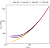 |
Fig. 2. Initial relaxation time as a function of radius, calculated from Eq. (3). |
| In the text | |
|
Fig. 3. Time evolution of the radial structure of the underfilling SCs (top row) and the filling SCs (bottom row). We show the core radius (as calculated by NBODY6++GPU), the 1% and 99% L.r., the half-mass radius, and the tidal radius (see also the legend). |
| In the text | |
|
Fig. 4. Total mass of the underfilling (left) and filling models (right) at time t, shown as a fraction of the initial SC mass, M0. |
| In the text | |
|
Fig. 5. Mean stellar mass in solar masses at time t in the underfilling (left) and filling models (right). The vertical axes have different scales. |
| In the text | |
|
Fig. 6. Time evolution of the Lagrangian radii of two stellar mass groups: low-mass (‘L’, m ≤ 0.2 M⊙, dotted lines) and high-mass (‘H’, m ≥ 0.9 M⊙, solid lines). The curves represent 1, 50, 75, and 90% of the total mass of the corresponding mass group (from bottom to top; the half-mass radius is also highlighted in red). The cluster tidal radius is the top dashed line. |
| In the text | |
|
Fig. 7. Evolution of mass segregation in the SCs. We compare the mean mass in the core and around the half-mass radius (crosses), and around the half-mass radius and in the outer regions (circles). The ranges of Lagrangian radii from which the mean mass is taken are specified as mass percentages in the labels. The underfilling models are shown in the left-hand panel, and the filling ones in the right-hand panel. |
| In the text | |
|
Fig. 8. Time evolution of β(r), defined by Eq. (1), in the underfilling models. The top row shows β calculated from the velocity dispersion of all stars in the SC (regardless of mass), and the rows below are calculated for specific mass groups – from the least massive in the second row, intermediate-mass in row three, and the most massive stars in the bottom row (see also the labels on the right-hand side). Red colours correspond to radial anisotropy, and blue colours to tangential anisotropy. If the fit is poorly defined because of an insufficient number of data points in a radius–mass bin, we mask the corresponding pixel in grey. To give a sense of the radial scale and dynamical evolution of the SCs in each plot, we also show the 1% L.r., the half-mass radius, the 99% L.r., and the tidal radius (from bottom to top; black lines). We note that because of the log-scale on the vertical axis, the bins below 2% may appear more prominent than the other bins despite covering a smaller radial range. |
| In the text | |
|
Fig. 9. Time evolution of the equipartition mass, meq, in the underfilling SCs (top row – calculated from the 3D velocity dispersion; middle row – calculated only from its radial component; bottom row – calculated only from its tangential component). The regions that evolve towards EEP (to lower positive values of meq) are in shades of blue and purple, and the regions that evolve away from EEP (to negative meq, i.e. away from EEP) are in shades of red; see the colour bars. To give a sense of the radial scale and dynamical evolution of the SCs in each plot, we also show the 1% L.r., half-mass radius, 99% L.r., and the tidal radius (from bottom to top; black lines). If the fit is poorly defined due to an insufficient number of data points in a radius–mass bin, we mask the corresponding pixel with grey. We note that because of the log-scale on the vertical axis, the bins below 2% may appear more prominent than the other bins despite covering a smaller radial range. |
| In the text | |
|
Fig. 10. Time evolution of the difference between the velocity dispersion of the high-mass stars (‘H’, 0.8 ≤ m/M⊙ ≤ 1.0) and that of the low-mass stars (‘L’, 0.1 ≤ m/M⊙ ≤ 0.2). The velocity dispersion is scaled by |
| In the text | |
|
Fig. 11. Same as Fig. 8 but for the filling models. The vertical axis has the same range as in Fig. 8 to ease the comparison; we note, however, that the tidal radius limits the SC at a much lower r. |
| In the text | |
|
Fig. 12. Same as Fig. 9 but for the filling models. The vertical axis has the same range as in Fig. 9 to ease the comparison; we note, however, that the tidal radius limits the SC at a much lower r. |
| In the text | |
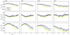 |
Fig. 13. Same as Fig. 10 but for the filling models. |
| In the text | |
Current usage metrics show cumulative count of Article Views (full-text article views including HTML views, PDF and ePub downloads, according to the available data) and Abstracts Views on Vision4Press platform.
Data correspond to usage on the plateform after 2015. The current usage metrics is available 48-96 hours after online publication and is updated daily on week days.
Initial download of the metrics may take a while.