| Issue |
A&A
Volume 691, November 2024
|
|
|---|---|---|
| Article Number | A202 | |
| Number of page(s) | 15 | |
| Section | Galactic structure, stellar clusters and populations | |
| DOI | https://doi.org/10.1051/0004-6361/202450783 | |
| Published online | 13 November 2024 | |
Energy equipartition in globular clusters through the eyes of dynamical models
1
Department of Mathematics and Physics, University of Campania Luigi Vanvitelli,
viale Lincoln 5,
81100
Caserta,
Italy
2
INAF – Osservatorio Astronomico d’Abruzzo,
Via M. Maggini,
64100
Teramo,
Italy
3
INFN – sezione di Roma,
Piazzale Aldo Moro 2,
00185,
Rome,
Italy
4
Department of Physics, University of Rome La Sapienza,
Piazzale Aldo Moro 2,
00185
Rome,
Italy
★ Corresponding author; This email address is being protected from spambots. You need JavaScript enabled to view it.
, This email address is being protected from spambots. You need JavaScript enabled to view it.
, This email address is being protected from spambots. You need JavaScript enabled to view it.
Received:
18
May
2024
Accepted:
1
October
2024
Abstract
Context. Following their birth, globular clusters (GCs) experience a very peculiar dynamical evolution. Gravitational encounters drive these systems toward energy equipartition, mass segregation, and evaporation, which alter structural, spatial, and kinematic features.
Aims. We determine the dynamical state of a few GCs by means of a multi-mass King-like dynamical model. Our work focuses on the prediction of the energy equipartition degree and its relationship with model parameters.
Methods. We adjusted the dynamical model parameters in order to reproduce the observed velocity dispersion – as derived from Hubble Space Telescope proper motion data – as a function of the stellar mass. By doing so, we estimated Φ0, a measure of the gravitational potential well. We repeated the same fit by means of the Bianchini relation, a function obtained by interpolating on N-body simulation results. We studied the relationship between Φ0 and the Bianchini equipartition mass meq and discuss the structural properties, such as concentration c, the number of core relaxation timescales Ncore, and core radius rc. To obtain an independent estimate of Φ0, we also fitted observed surface brightness profiles using the predicted surface density and a mass-luminosity relation from isochrones.
Results. The quality of the fits of the velocity dispersion–mass relationship obtained by means of our dynamical model is comparable to those obtained with the Bianchini function. Nonetheless, when the Bianchini function is used to fit the projected velocity dispersion, the resulting degree of equipartition is underestimated. On the contrary, our approach provides the equipartition degree at any radial or projected distance by means of Φ0. As a result, a cluster in a more advanced dynamical state shows a larger Φ0, as well as larger Ncore and c, while rc decreases. We find the estimates of Φ0 obtained by fitting surface brightness profiles to be compatible at 2σ confidence level with those from internal kinematics, although further investigation of statistical and systematic errors is required.
Conclusions. Our work illustrates the predicting power of dynamical models to determine the energy equipartition degree of GCs. These models are a unique tool for determining structural and kinematic properties, and can be used where observational data are poor, as is the case for the most crowded regions of a cluster, where stars are barely resolved.
Key words: stars: kinematics and dynamics / globular clusters: general
© The Authors 2024
 Open Access article, published by EDP Sciences, under the terms of the Creative Commons Attribution License (https://creativecommons.org/licenses/by/4.0), which permits unrestricted use, distribution, and reproduction in any medium, provided the original work is properly cited.
This article is published in open access under the Subscribe to Open model. This email address is being protected from spambots. You need JavaScript enabled to view it. to support open access publication.
1 Introduction
Searching in the vicinity of the Milky Way, we find mostly spherically shaped stellar systems with an increasing density of stars toward their center. These are called globular clusters (GCs). They are commonly known for their very old age, which reaches ∼10 Gyr in most cases or even more.
GCs were thought to consist of a single stellar population with low metallicity. However, the detection of chemical and photometrical differences first suggested and then confirmed the presence of different generations of stars. A variety of questions were raised, establishing a renewed interest in GCs. Astronomers are studying the possible formation scenarios of such multiple stellar generations, as well as their initial properties, using the enormous amount of recently collected observational data and by developing advanced models (see the reviews by Bastian & Lardo 2018; Gratton et al. 2019; Milone & Marino 2022). Behind their intriguing formation and stellar generations, GCs have a highly articulated dynamical evolution. Their high-density environment makes them the only known collisional star-cluster systems in astronomy. The relaxation process driven by gravitational encounters between stars plays a fundamental role in determining the structure and evolution of GCs following their birth. The efficiency of relaxation brings these systems toward a degree of kinetic energy equipartition among stars (Spitzer 1987), altering their structural and kinematic features. Such internal dynamical processes affect the spatial distribution of stars, a phenomenon known as mass segregation. A system close to equipartition has massive stars with a lower velocity dispersion, which consequently sink toward the center. On the contrary, less massive stars are faster and migrate to the outer regions. Here, the gravitational pull of our Galaxy subtracts stars from the cluster, leading to a limited phase-space domain through what is known as evaporation (Ambartsumyan 1938; von Hoerner 1957; King 1958a,b; Spitzer 1987), and producing the tidal streams (Odenkirchen et al. 2001; Piatti & Carballo-Bello 2020). The joint effect of mass segregation and evaporation flattens the mass function, whose initial shape is largely unknown. Our comprehension of the internal dynamics of GCs can provide hints concerning their initial mass function (IMF). The mass loss from GCs following their formation also contributes to populating the Galactic environment. Depending on their orbits, they can suffer shocks and inhomogeneities in the still unknown early galactic potential (Webb et al. 2019). Regarding multiple stellar generations, these dynamical processes, coupled with stellar evolution, favor a strong and predominant loss of first-generation stars in the early evolutionary phases of clusters. The evaporation of such stars may explain the origin of galactic halo stars. Furthermore, the internal dynamics mixes these populations, mainly erasing their initial spatial and kinematic differences, further complicating attempts to understand the characteristics of the system. Studying GC dynamics can thus reveal fundamental insights concerning the early environment of our Galaxy, as well as their contribution to its evolution (see Chapter 8 of Gratton et al. 2019).
Although it is well known that massive stars are more centrally concentrated than less massive ones, a theoretical description of energy equipartition, mass segregation, and evaporation is still missing and astronomers are trying to quantify these processes. A satisfying explanation of this intricate stellar dynamics is required to extract information about the primordial environment and the formation scenario of GCs. Understanding the stellar dynamics may also help to solve the puzzle of the formation of multiple stellar generations, describing their dynamical evolution. However, even single stellar population dynamical phenomenology still needs to be fully understood.
Focusing on energy equipartition, several scientists are exploring GC evolution through N-body simulations to study the efficiency of this process and its relation to structural and internal properties, as well as initial conditions (Trenti & van der Marel 2013; Webb & Vesperini 2017; Pavlík & Vesperini 2021b,a, 2022). Among such works, the most important from our perspective is that of Bianchini et al. (2016). Here, with a set of N -body simulations, the authors look at the degree of energy equipartition through the velocity dispersion as a function of stellar mass in the inner regions of clusters (namely inside the half-mass radius). These authors find an analytic formula to fit the velocity dispersion–mass relationship that is
 (1)
(1)
where the equipartition mass meq is the parameter that quantifies the degree of energy equipartition, while σ0,B is a normalization constant and σeq = σ0,B exp (−1/2). In a subsequent paper, Bianchini et al. (2018) characterize the variation of meq during GC evolution and its dependence on the radial coordinate.
The provided fitting function includes the limit of complete equipartition for masses m > meq, which is σ(m) ∝ m−1/2. Then, meq tells us which masses reach complete equipartition, with high-mass stars closer to equipartition than low-mass stars. Furthermore, as the degree of equipartition is expected to increase with the dynamical state of a cluster, the meq parameter appears to be related to the concentration parameter c and the numbers of relaxation times elapsed during the life of a cluster, namely Nrelax = tage/trelax, where tage is the age of a cluster and trelax is the relaxation time, which is often evaluated in the core trc and at the half-mass radius, yielding the number of core and median relaxation timescales Ncore and Nhalf respectively (Bianchini et al. 2016). The work of these authors has gained attention in the literature due to the simplicity of the analytical function. It was used in N -body simulations to quantify the degree of energy equipartition in GCs hosting multiple stellar populations (Vesperini et al. 2021) and to explore the effect of anisotropy, primordial binaries, tidal field, and black holes in equipartition (Pavlík & Vesperini 2021b,a, 2022; Aros & Vesperini 2023). The exponential fitting function in Eq. (1) is often compared with the classical power law σ(m) = σs(m/ms)−η with η = 0.5 for complete equipartition, where σs and ms are scale values for the velocity dispersion and mass.
Thanks to Hubble Space Telescope (HST) proper motion measurements, observers can now both measure internal kinematics and estimate stellar masses, quantifying the equipartition level in a few GCs (Libralato et al. 2018, 2019, 2022). In Watkins et al. (2022, hereafter W22), the authors analyzed the degree of energy equipartition in nine GCs using the Bianchini et al. (2016) fitting function and the classical one, with the respective parameters. Most, if not all, of the stars of the studied clusters do not show complete equipartition.
Although the Bianchini function reproduces the observable well, it provides no information on the physics underlying the equipartition process. Our aim is to compare measured data and the Bianchini fitting function with theoretical results, which provide more fundamental information about cluster dynamics. Multi-mass King-like dynamical models have the advantage of being self-consistent, that is they are directly obtained from the physics of the system, namely the gravitational interaction between stars, the mass distribution, and the limited available phase space. As a consequence, the dependence of the velocity dispersion on mass is predicted by the model itself, and is not related to an interpolation function that fits simulation outputs and observations. In this paper, we carefully discuss the relation between the outcomes of our model and N-body-based results, namely the successful Bianchini fitting function. We note that N-body simulations are used to study the temporal evolution of stars in clusters, numerically integrating the Newtonian equation of motion after choosing suitable initial conditions. Current state-of-the-art simulations include a variety of phenomena, such as the treatment of stellar evolution, binary systems, compact object formation, and tidal forces, which make them a powerful numerical tool for simulating more realistic clusters. However, the definition of such recipes and the choice of initial conditions themselves require accurate modeling. Theoretical assumptions and prescriptions can significantly affect the simulation results. This is why most researchers explore the parameters of those models to determine the initial conditions and to describe the considered phenomena. As a result, N-body methods are a modeling tool needed to explore the temporal evolution, but they require theoretical references to consistently set up the simulations themselves. Despite large increases in computational resources in recent years, realistic simulations require large and advanced computer infrastructures as well as computational time, which grows with the square of the number of simulated stars.
On the contrary, exploring dynamical models for GCs is much less computationally expensive. In our approach, a single equilibrium configuration can be obtained in few seconds or minutes depending on the desired precision. Furthermore, these models can be used to predict radial and projected profiles for several observables, such as the surface density (both in mass and in the number of stars), the surface brightness (if a mass– luminosity relation is known), and the velocity dispersion. When using models including a mass distribution, our knowledge of the distribution function characterizes not only the phase-space but also the mass function. These models provide a description of the seven-dimensional space of masses, positions, and velocities. Such theoretical frameworks are clearly limited by the assumptions made, as in our case where isotropic velocities are considered. Furthermore, some theoretical quantities require observational constraints in order to get their numerical values, as is usually the case for physical models. The temporal evolution is assumed as described by equilibrium configurations with different structural parameters, whose values determine the dynamical state. The temporal dependence of such quantities can be addressed with numerical simulations, which offer a unique opportunity in that sense (see Wang et al. 2016, for a relation between the King single-mass model parameter W0 and advanced simulations). Indeed, observing the historical properties of GCs would require observations of the satellites of distant galaxies (i.e., far enough to look back in time into the life of the GCs) under the strong assumption that cluster evolution is similar in every galactic environment, which may not be the case. Unfortunately, we are currently limited to GCs of the Milky Way and its satellites and nearby galaxies.
Numerical simulations and theoretical modeling can therefore provide a broader perspective as to the dynamics of GCs. However, we strongly emphasize that taking advantage of dynamical models is fundamental to understanding the underlying physics of the processes involved. Such models are an advanced interpretative and predictive tool for addressing the major open questions in the field.
2 Methods
Our main approach consists in comparing the velocity dispersion dependence on stellar mass predicted by our multi-mass dynamical model for GCs, with the Bianchini function in Eq. (1), fitting the observational data by W22. The fitting procedure leads to an estimate of model parameters, to be related with the Bianchini equipartition mass meq.
We also look at the surface brightness profiles (SBPs) of the clusters by fitting the measured data by Trager et al. (1995) with our theoretical prediction, which provides an estimate of parameters from a different observable. This allows us to see how confident our model is at reproducing both the observed internal kinematics and luminosity profile.
2.1 Dynamical model
Our dynamical model derives from the distribution function (DF) obtained by King (1965) as an approximated solution of the Fokker-Planck equation, which itself comes from the Boltzmann equation for collisional systems (Chandrasekhar 1943; Rosenbluth et al. 1957; Spitzer & Härm 1958; Chandrasekhar 1960). The King model (King 1966) was a single-mass one, with the DF having a cut-off in the phase-space that takes the Galactic tidal field into account. Such a model describes the equilibrium configuration of the system, once the DF is used to calculate the density profile and solve the Poisson equation for the gravitational potential. It was used for many years by astronomers to fit the SBPs of GCs and to obtain structural parameters (Peterson & King 1975; Trager et al. 1995; Harris 1996; Miocchi et al. 2013). A further step on was done first by Da Costa & Freeman (1976), introducing a discrete multi-mass model with ten mass classes, each having its own DF with an energy cut-off and a weight factor to be constrained by observations. They successfully fit M3 surface brightness, where the King model was failing to reproduce both the inner and outer profile.
Due to the general good agreement between the King model and observations, little effort was put in developing and exploring multi-mass models, although they are fundamental in the comprehension of several phenomena produced or altered by the mass distribution, like segregation, evaporation, and equipartition (Miocchi 2006; Gieles & Zocchi 2015; Peuten et al. 2017; Torniamenti et al. 2019; Dickson et al. 2023). Even if N-body simulations are offering great opportunities in understanding the dynamical evolution of GCs, we underline the importance of developing analytical models to describe physical processes, offering an important tool in the comprehension of such systems, like it was the King DF.
The formulation of a continuous multi-mass model was presented by Merafina (2019), as an extension of the Da Costa & Freeman one and recovering the King formalism. The model we present is similar, but with some improvements concerning the derivation and the relation with the global mass function. Our DF is an approximated solution of a generalized expression of the Fokker-Planck equation, valid for collisional systems with a mass distribution (see Eq. (A.1)). The DF keeps the property of being limited in the phase-space. Moreover, not only it brings information on the velocity distribution within the cluster, but it also concerns the mass distribution of the stars, meaning that the mass function is embedded in the DF. Its expression is
![Mathematical equation: $g(r,v,m) = k(m){{\rm{e}}^{ - m\left[ {\varphi (r) - {\varphi _0}} \right]/\left( {{k_{\rm{B}}}\theta } \right)}}\left[ {{{\rm{e}}^{ - \varepsilon (v,m)/\left( {{k_{\rm{B}}}\theta } \right)}} - {{\rm{e}}^{ - {\varepsilon _{\rm{c}}}(r,m)/\left( {{k_{\rm{B}}}\theta } \right)}}} \right],$](/articles/aa/full_html/2024/11/aa50783-24/aa50783-24-eq2.png) (2)
(2)
where ε = mv2/2 is the kinetic energy of a star with mass m and εc = mv2/2 is its cut-off energy with ve = ve(r) the escape velocity, φ(r) is the gravitational potential (with φ0 its value in the cluster center) and r is the radial coordinate. The variable θ is the thermodynamic temperature, a memory of the Boltzmann DF limit and constant all over the equilibrium configuration (Merafina 2017; Merafina 2018, 2019) and kB is the Boltzmann constant. The multiplying factor k(m) weights the DF of each mass m, like it was in the Da Costa & Freeman (1976) model, although theoretically it gathers some mass-dependent functions resulting from the derivation, related with the mass function and the escape velocity at cluster center (see Appendix A for details).
The mass density radial profile ρ(r) is computed through an integration over the masses and velocities of the DF in Eq. (2), that is
![Mathematical equation: $\rho (r) = \int_{{m_{\min }}}^{{m_{\max }}} {\left[ {\int_0^{{v_{\rm{e}}}(r)} g (r,v,m){{\rm{d}}^3}v} \right]} {\rm{d}}m,$](/articles/aa/full_html/2024/11/aa50783-24/aa50783-24-eq3.png) (3)
(3)
with mmin and mmax the extremes of the mass range, where the mass function is valid. Equation (3) is used to solve the Poisson equation for the gravitational potential. Following the King formalism, one could introduce ![Mathematical equation: $W(r) = {\varepsilon _{{\rm{c}},1}}(r)/\left( {{k_{\rm{B}}}\theta } \right) = {m_1}v_{\rm{e}}^2(r)/\left( {2{k_{\rm{B}}}\theta } \right) = {m_1}\left[ {{\varphi _{\rm{R}}} - \varphi (r)} \right]/\left( {{k_{\rm{B}}}\theta } \right)$](/articles/aa/full_html/2024/11/aa50783-24/aa50783-24-eq4.png) and solve the Poisson equation for W(r), obtaining a set of equilibrium configurations each identified by the initial condition W0,1 = m1 [φR − φ0] /(kBθ), like shown in Merafina (2019). However, the parameter for determining the configuration should not depend on the scale mass (the models by Da Costa & Freeman 1976 and Merafina 2019 were using the greatest mass m1 of the system). Using a generic mass unit mu and solving for Wu(r) = mu[φR − φ(r)]/(kBθ), the expression of the dimensionless Poisson equation keeps the same analytical expression, that is
and solve the Poisson equation for W(r), obtaining a set of equilibrium configurations each identified by the initial condition W0,1 = m1 [φR − φ0] /(kBθ), like shown in Merafina (2019). However, the parameter for determining the configuration should not depend on the scale mass (the models by Da Costa & Freeman 1976 and Merafina 2019 were using the greatest mass m1 of the system). Using a generic mass unit mu and solving for Wu(r) = mu[φR − φ(r)]/(kBθ), the expression of the dimensionless Poisson equation keeps the same analytical expression, that is
 (4)
(4)
with the dimensionless coordinate x = r/rk,u in units of the King radius  . The initial conditions of Eq. (4) are
  and Wɪ(x = 0) = W0,u = mu(φR −φ0)/(kBθ), which determines the solution. Here, we use a better parameter to identify the equilibrium configuration, that is Φ0 = (φR − φ0)/(kBθ), which measures the potential well without depending on a scale mass (as W0,u do) and having the dimension of the inverse of a mass.
To solve Eq. (3), the quantities in the DF in Eq. (2) must be known. At the present state of development, the factor k(m) has to be constrained from the global mass function ξ(m) with a numerical procedure. Since the integration of g(r, v, m) over the radial coordinate r and the velocity v gives the mass function by definition, we can iteratively constrain k(m). In this work, we consider a single-power law mass function ξ(m) ∝ mα , with the slope α taken from Baumgardt et al. (2023) or theoretically assumed. The code that numerically integrates Eq. (3), once given the slope α, the mass range and Φ0, evaluates k(m) with a convergence procedure and draws radial profiles for each mass composing the system. These include the 3D velocity dispersion profile as function of mass
 (5)
(5)
that we project in two dimensions to obtain σ(R, m), with R the projected distance from the cluster center. This profile is needed to fit the proper motion observations on σ(m).
The model also provides the density profile of each mass, which is used to predict the surface density profile for each mass Σ(R, m), by integrating along the line of sight. This allows us to estimate the surface brightness profile I(R), by introducing a mass-luminosity relation. This is a fundamental step when dealing with multi-mass systems in particular. We go through the details of the production of the theoretical SBPs in Sect. 2.2.2, where we discuss the fitting procedure on observational data.
2.2 Fitting procedure
2.2.1 Velocity dispersion–mass relationship
W22 provide the binned velocity dispersion of stars as function of their estimated mass for a sample of Galactic GCs (see their Table 2). Their dispersion measures are obtained from proper motion (then in the 2D plane of the sky) and inside a ring in the inner regions of the analyzed clusters.
In order to compare the model prediction with the data, we compute σ(m) from the projected profile σ(R, m) in the same region. When looking at a projected radial distance from cluster center R, the observer intercepts all stars having 3D radius r ∈ [R, Rt], where Rt = rt is the tidal radius. Then, we average the 3D profile σ(r, m) in that range to obtain the 2D profile σ(R, m). Subsequently, the projected dispersion is averaged in the circular annulus covered by the data sample, drawn around the median radius (see W22, Table 1). We use the observed core radius rc from the Harris (1996) catalog (2010 edition, hereafter indicated as the Harris catalog) and the theoretical core radius rc,th to convert the dimensional coordinates into our dimensionless ones. Here, rc,th is obtained from the surface density profile, predicted by our model. This coincides with rc if the surface brightness profile is proportional to the surface density profile (with a factor only dependent on mass).
The overall average procedure returns the velocity dispersion as function of stellar mass, normalized to the dispersion of the lowest mass σ0 . The shape of σ(m)/σ0 depends on the model parameters. In particular, for an increasing Φ0 that gives a more advanced dynamical state, the dispersion σ(m) is closer to the complete energy equipartition limit σ ∝ m−1/2. Furthermore, more massive stars have a greater degree of equipartition than less massive ones for any value of Φ0 (see Fig. B.5 available on Zenodo).
Concerning the choice of the mass function shape needed to draw theoretical profiles, we set mmin = 0.1 and mmax = 1.0, while for the slope α we select two approaches: the first takes it from Baumgardt et al. (2023), the second one (more general) explores a wide range α ∈ [−2.0, 0.0], actually adding the slope to the parameter space of the minimization procedure. As a consequence, the first approach gives the best-fit values of σ0 and Φ0, while the second also returns an estimate for α. For the fit, we numerically minimize the χ2 test value between data and model prediction. We apply this procedure to the GCs in our sample, only removing NGC 2808 following W22. We also fit the velocity dispersion data with the Bianchini function in Eq. (1), to have an estimate of the χ2 , to be compared with our model ones. Although such a fit is less detailed than in W22, we obtain the Bianchini equipartition mass meq and the normalization constant σ0,B .
2.2.2 Surface brightness profiles
An extensive catalog of SBPs for Milky Way GCs was released by Trager et al. (1995). Although more accurate measurements are available from the work conducted by Noyola & Gebhardt (2006) with HST photometry, they are restricted to internal regions and to a few subsets of clusters. For these reasons, we choose the Trager et al. (1995) dataset. To analyze the profiles, we follow a procedure similar to that described by McLaughlin & van der Marel (2005) and Zocchi et al. (2012), which these authors used to estimate uncertainties on the data and fit SBPs with single-mass dynamical models. The Trager et al. (1995) SBPs consists of measurements for the logarithm of the projected radial coordinate Ri, the surface (apparent) magnitude in the V -band µV (Ri), as well as its best-fit with Chebyshev polynomials and a weight wi for each point according to its by-eye reliability. The analysis performed by McLaughlin & van der Marel (2005) provides an estimate of the uncertainty for each surface brightness measure, namely δµV(Ri) = σµ/wi, where σµ is a constant that varies from cluster-to-cluster. Following Zocchi et al. (2012), we remove data points with wi < 0.15 and we correct each measure for the extinction as derived from the Harris catalog.
In the context of multi-mass dynamical models, the standard assumption of a constant mass-to-light ratio is too crude. To obtain the theoretical profile for the surface brightness, useful to fit the available data, we need a mass-magnitude relation in the V -band. Using theoretical isochrones we can establish such a relationship by assigning to the masses of the dynamical model a value for the corresponding absolute magnitude MV . We use BaSTI isochrones (Hidalgo et al. 2018; Pietrinferni et al. 2021; Salaris et al. 2022; Pietrinferni et al. 2024), considering an age of 13 Gyrs, [α/Fe] = +0.4, the He mass fraction Y = 0.247 and a different metallicity [Fe/H ] for each cluster as a reference case. The metallicity value is taken from the Harris catalog, where we also get the distance modulus to convert the observed apparent magnitudes into absolute ones. Due to stellar mass loss, the final mass of each star is naturally different from its initial mass, depending on its evolutionary state. In particular, initially more massive stars are now much brighter than low-mass stars, even if their current mass may be similar. Furthermore, since GCs are very old, and excluding remnants, the most massive stars have around 0.8 M⊙ and their mass loss occurred mainly in the last million years. As a consequence, they did not have the time to adjust their dynamical state, which is better described by their initial mass. We then use the initial mass as representative of the dynamical mass, in order to assign the corresponding MV value. We note that when the stars evolve beyond the main sequence, a large variation in luminosity occurs for a very small variation in their mass. These evolved stars are also the more massive ones still alive in the cluster. For these reasons, they play an important role in shaping the surface brightness profile in the more central regions of clusters, because of the mass segregation process. To account for these effects, we choose a regular mass step, but substantially smaller than that used to determine the velocity dispersion. We note that the mass range, in particular the maximum mass of stars still alive, is provided by the isochrones and depends on the age of the cluster. While this maximum mass has a little effect on the prediction of σ(m), it will play an important role in shaping the surface brightness profile.
Finally, we follow Zocchi et al. (2012) regarding the minimization procedure of the χ2, by converting both the observed and the theoretical SBPs into solar luminosities.
Concerning the theoretical prediction, the model gives the surface density profile for each mass Σ(R, m). The global SBP I(R) is defined as
 (6)
(6)
where LV is the luminosity obtained by converting the theoretical absolute magnitudes MV to solar luminosities, using MV,⊙ = 4.83 (see the Sun Fact Sheet by NASA). Although MV,⊙ may suffer from several non-negligible uncertainties, as noted by Torres (2010), its choice is irrelevant in our fits.
The computed theoretical profile is normalized to its central value I0. The shape of I(R)/I0 depends on the parameters of the model, and its values are given for the dimensionless radial coordinate. However, in our fitting procedure, we must be aware that the observed radial coordinate is in physical units. To deal with all these, we define a numerical auxiliary function h(R/Rc; Φ0,α, mmin, mmax) = I(R)/I0 where Rc is the core radius, α is the mass function slope that we take from Baumgardt et al. (2023), mmin and mmax are the mass extremes given by the isochrone. We numerically minimize the χ2 and obtain an estimate of the best-fit Φ0, I0 and Rc . On the theoretical ground, since the 2D and 3D radial grids are the same, rc = Rc and rt = Rt. We apply this method to each cluster for which we have analyzed the velocity dispersion–mass relation. In this way, we can obtain two independent estimations of the Φ0 parameter.
2.3 Error estimation
Our fitting procedure is based on the χ2 minimization with respect to parameters. In our modeling for the velocity dispersion-mass relation, such parameters are Φ0 and σ0 for the first approach, while the second one also includes the slope α. The minimization of the χ2 requires that дχ2/дaj = 0 and д2χ2/дaiдaj < 0 where aj represents the parameters. We obtain such conditions with a numerical procedure. For the uncertainties, we need to compute the matrix Mij = (1/2) д2χ2/дaiдaj, whose inverse M−1 is the covariance matrix, from which we obtain parameters errors  as well as error bands for the velocity dispersion. A similar procedure is done when the slope is considered as a free parameter.
Our theoretical prediction for the velocity dispersion as function of stellar mass depends on parameters. We can write that σ(m; Φ0, σ0) = σ0f(m; Φ0) where f(m; Φ0) is the numerical relation obtained from the model (that generally also depends on α, fixed in the first approach). To obtain the matrix M, we must compute the derivative of the χ2 with respect to parameters. Specifically, we have an analytical expression for the first and second derivatives with respect to σ0. Concerning the derivatives with respect to Φ0, we use the Finite Difference Methods for their approximation. For the first derivative, we use
 (7)
(7)
where ΔΦ0 is the numerical step in Φ0 used to compute the function f . Regarding the second derivative, we take
 (8)
(8)
Both approximations are considered at second order. When the slope is added to the parameter space, we have σ(m; Φ0, α, σ0) = σ0 f (m; Φ0, α). For the derivatives with respect to the slope, we consider the same Finite Difference Eqs. (7) and (8) for their approximation, using the numerical step Δα. The mixed derivatives are obtained similarly, applying the same method.
Concerning the fitting procedure on SBPs, we follow the same approach. We determine the covariance matrix by computing (and inverting) Mij = (1/2) д2χ2/дaiдaj where the parameters are Φ0, Rc and I0. Except for the latter that has an analytical expression, the first, and second derivative of the χ2 with respect to Φ0 and Rc need the derivatives of I(R) with respect to the same parameters. These are approximated by using the Finite Difference Method, similarly to what already described, as well as for mixed derivatives. We obtain uncertainties δΦ0 , δI0 and δRc , from which we can also compute the uncertainty on the tidal radius.
3 Results
We report here the main results concerning our fit of the projected velocity dispersion as function of stellar mass. The estimated model parameters are given and the relation between Φ0 and the equipartition mass meq is shown and discussed. The relations with GCs structural parameters are also presented.
Finally, we show the estimated Φ0 parameter by fitting the SBPs and compare them with the values obtained by fitting the σ(m) observable.
3.1 Fitting the velocity dispersion to constrain Φ0
As a first approach, we evaluate Φ0 by fitting the velocity dispersion data with the model prediction, considering a single power law mass function ξ(m) ∝ mα with the slope α taken from Baumgardt et al. (2023), but with a mass range 0.1 < m/M⊙ < 1.0, slightly broader than the usual one [0.2, 0.8] M⊙. However, it can be shown that the effect of a different range of masses (when reasonable) is negligible with respect to variations in Φ0 or α.
In Fig. 1 we plot σ(m) predicted by the model against dispersion data by W22 and the fit with the Bianchini function for NGC 6397.
The plot clearly underlines a great compatibility between the model prediction and the Bianchini fitting function on the same data. We confirm a partial degree of equipartition in all clusters and for all masses (see also Fig. B.1 for other clusters). We expect that a cluster in an advanced dynamical state is closer to energy equipartition and shows a smaller value of meq . In the model framework, dynamically old means a greater Φ0 value, namely a deeper gravitational potential well. Then, there should be a relation between these parameters: a cluster showing a higher degree of equipartition should have a greater value of Φ0 and a lower value of meq . This is what we obtain in Fig. 2, where we plot the relationship between meq by W22 and the estimated Φ0, colored with the obtained χ2 . In Table 1 we give the estimated parameters and the χ2 test value for all analyzed clusters, also for our fit with the Bianchini fitting function. Our evaluation of meq , conducted on binned data and with a nonlinear least squares algorithm (available in the SciPy software package), is similar to that obtained by W22, who used unbinned data, set prior constraints on the parameter values, and used a Monte Carlo method to sample the parameter space. The χ2 values of the two fits are close to each other, sustaining a similar confidence with the data. Furthermore, the scaling dispersion σ0 of our model is systematically lower than σ0,B , a natural behavior due to the different meaning they have. While the first is the dispersion of the lowest model mass, the latter is the dispersion value in the limit m → 0.
The results of the fits made by using the classical power law σ(m) = σs(m/ms)−η, with ms = 1.0 M⊙, are shown in Table 2.
Our estimates of η, obtained with the same method as for meq , are compatible with those provided by W22, statistically equivalent to the other fitting functions, with small variations in the obtained χ2 . Furthermore, η follows the expected trend with meq and Φ0 . For a more advanced dynamical state, we have a larger degree of equipartition described by a higher η value, as well as a larger Φ0 and a smaller meq , as expected. W22 already provided a discussion of the relationship between the classical power law and the Bianchini fitting function, as well as the obtained values for the equipartition mass and η, showing that they appear equivalent in measuring the equipartition degree. Here we focus on the link between the Bianchini function and the dynamical model prediction due to the closer statistical compatibility obtained in our fits.
Concerning the results of the fitting procedure and the relation between meq and Φ0 , some considerations must be made. First, for NGC 5139 (ω-Cen) we have the lowest value of Φ0 and the greatest value of meq, also coming with a very poor fit quality (largest χ2 value). This cluster must be treated with caution due to its intricate history and structure. It shows evidence of multiple stellar populations that are dynamically interacting and are likely to have different degrees of equipartition. Furthermore, each has its own mass function and chemical pattern. It is also strongly suspected to be the survived core of a disrupted dwarf galaxy. The full picture behind this object requires further study with more sophisticated models, given its complexity. Although the overall trend for σ(m) looks promising, we emphasize that the uncertainties may be underestimated due to the fluctuations around the decreasing pattern (we come back to this point in the next lines). This suggests an additional source of statistical error that may increase the estimated uncertainty in the corresponding Φ0 value. However, the long relaxation timescale of such a cluster (see Table 1 in W22 work) may indicate that our estimates are not far from reality, specifically a low energy equipartition level corresponding to a smaller Φ0 and a larger meq . Furthermore, NGC 6397 and NGC 6752 are post-core collapsed objects according to the Harris catalog, since they have a very high value of the concentration, while NGC 6266 is suspected to be collapsed even if its concentration is not very high. Considering that only for three of the analyzed clusters, namely NGC 6266, NGC 6341 and NGC 6397, we have a high confidence level coming from the fitting procedure, excluding collapsed objects and poor fit quality results, we are left only with NGC 6341, which is also the cluster with the lowest meq and the highest Φ0 . Moreover, this cluster has a low mass coverage in the velocity dispersion data, with a range of 0.59 < m/M⊙ < 0.78. Looking at data points (see Fig. B.1), it looks evident a decreasing trend of σ(m) with the mass, but the oscillations around such tendency, which change from cluster to cluster, suggest that uncertainties can be underestimated. Indeed, we obtain a relation between our χ2 test value and the average relative error on σ(m) data (see Fig. B.4), showing that low relative errors produce a greater χ2 value in our fitting procedure (with ω-Cen showing the lower relative error and the larger χ2), while the opposite is vaguely true for greater relative errors. Furthermore, our χ2 looks slightly asymmetric with respect to Φ0 in the minimum, suggesting a more advanced uncertainty estimation method for such parameter, like evaluating the right and left errors. However, this does not affect the results that we present here.
The uncertainties given for Φ0 reflect the observed ones and come from the minimization process. A possible source of error in our procedure is the choice of the core radius. It can affect the theoretical prediction, since it determines the radial shell where the projected velocity dispersion σ(R, m) is averaged (see Sect. 2.2.1). An underestimation of the core radius would map the observed radial shell into a more outer dimensionless radial shell. As a result, the velocity dispersion would be generally smaller and more dominated by the low-mass stars due to mass segregation. Then, σ(m) would be steeper and the corresponding best-fit Φ0 would be higher. The opposite holds for an overestimate of the core radius. This introduces a systematic error into our procedure for determining model parameters, but we do not explore such an effect here. Actually, the expected relation between Φ0 and rc suggests that only a large relative uncertainty on the core radius may affect the estimate of Φ0 . We quantify the effect of varying rc on the Φ0 determination in Sect. 3.4.
All these uncertainties motivate an independent examination of Φ0 , as obtained by fitting the surface brightness profile (see Sect. 3.5).
Consequently, our work must be considered as a first guess in the evaluation of multi-mass dynamical model parameters from GCs kinematic observations concerning energy equipartition.
Outline of parameters for the analyzed GCs.
Estimated parameters for the classical power law.
 |
Fig. 1 Projected velocity dispersion as a function of stellar mass for NGC 6397. The error bars are the data from Watkins et al. (2022), the continuous green line is our best fit with the Bianchini et al. (2016) fitting function in Eq. (1) with its error band, the dotted brown line is the complete equipartition limit (σ ∝ m−1/2), and the dashed orange line is our model best-fit with its 68% confidence band. |
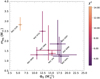 |
Fig. 2 Relation between the estimated Φ0 and meq from Watkins et al. (2022). The χ2 test value is given by the color of the data point for each NGC according to the color bar to the right. |
3.2 Adding the mass function slope to the parameter space
As an extension of the previous analysis, we add to the parameter space the mass function slope α. The fitting procedure is naturally more computationally expensive, because we have to iteratively solve equilibrium configurations with a different mass function. As previously done, we minimize the χ2 for each cluster: we explore Φ0 around a value close to the one obtained with the first approach and the slope α is taken in the range [−2.0, 0.0]. The adopted range for α accounts for the typical slopes values of GCs and is only a first guess, to be eventually modified to increase the precision. Unfortunately, we find a degeneration between Φ0 and α, preventing a more precise evaluation of the slope.
In Fig. 3, we show the contour plot for NGC 6397 in the Φ0–α plane, with some values around the χ2 minimum, together with the mass function assumed in the first approach, with its uncertainty. Even if our minimum falls in the error band by Baumgardt et al. (2023) for NGC 6397, the same is not valid for other clusters (see Fig. B.2). Furthermore, the shape of the parameter space is preventing us to constrain the slope of the mass function, whose uncertainties are too big and overcome the considered range. In Table 3 we give the results for the estimated model parameters, with their errors.
Although the contour plots are not the same for all analyzed clusters, in some cases there is a small tendency of having a greater Φ0 corresponding to a lower α, while in other ones the contour plot lines are almost horizontally oriented. Indeed, the velocity dispersion dependence on mass is steeper and closer to equipartition for both a larger Φ0 or a greater slope α. Such effect is expected since a larger slope means a flatter mass function, with more massive stars than a steeper one. This results in a greater degree of energy equipartition, because massive stars are more efficient in reaching equipartition due to their higher mass, which cause them to suffer more gravitational encounters than less massive stars. Similarly, a greater Φ0 implies a deeper potential well, namely a more dynamically evolved cluster, with a higher level of equipartition. As a result, a given degree of equipartition can be reached with more massive stars and a less deep gravitational well or by a stronger gravity and a steeper mass function. However, the effect of the gravitational potential through the Φ0 parameter looks more important, with smaller changes affecting equipartition more than variations in the slope. This is also remarked by the estimated errors on Φ0 , which are compatible with respect to the first approach, meaning that any reasonable assumption on the mass function slope would work well in setting up the model and constrain Φ0 from the velocity dispersion σ(m).
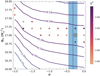 |
Fig. 3 Contour plot for NGC 6397 in the Φ0−α plane, showing the χ2 levels. The blue band gives the slope from Baumgardt et al. (2023). Squares indicate the χ2 values around the minimum, which is identified by a large gray circle. |
Results of the second fitting approach.
 |
Fig. 4 Radial and projected profile of the equipartition mass meq, obtained by fitting the model prediction of the velocity dispersion with the Bianchini function at each radial coordinate, given in units of the core radius. The panel zooms onto the region r ≤ rc. |
3.3 Shell selection and projection effects
As already outlined, the data we are fitting concerns projected quantities, and it is restricted to a circular ring close to the central regions of the clusters. We explore, by means of our model and the Bianchini fitting function, the effects of projection and shell selection in quantifying the degree of equipartition.
Our dynamical model predicts the shape of the function σ(r, m), which can be used to explore the degree of energy equipartition in different radial shells. Equipartition is more efficient in the core of clusters, and the maximum degree is expected to be measured there. Unfortunately, to date kinematic measurements in the core are difficult due to crowding effects and are limiting observers to look around it, as W22 do. As a result, the measured degree of equipartition is less than the core one. Furthermore, working with projected velocities also gives a smaller equipartition level than using 3D quantities. Indeed, at the projected radial distance R, the observer intercepts stars with a 3D radial distance r є [R, rt]. Being the velocity dispersion σ(r, m) a decreasing function of r, its value is lowered for each mass, in average, with respect to the 3D one. Being massive stars more centrally concentrated than less massive ones, the projection decreases more σ(m) for low-mass stars and brings to a flatter profile, resulting in a lower equipartition degree with respect to the 3D case. Both these effects bias the estimation of meq, leading to higher values (i.e., lower equipartition). To visualize this, we plot in Fig. 4 the value of meq obtained by fitting with the Bianchini function the 3D and 2D theoretical profiles σ(r, m) and σ(R, m) respectively, for a particular choice of α and Φ0. Such analysis is possible due to the very good similarity between our prediction for σ(m) and Eq. (1), which we check quantifying the uncertainty of the fitted meq and verifying its small value.
As expected, meq increases with the distance from the center of the cluster, due to the decreasing efficiency of the relaxation process. A measure of the maximum degree of equipartition should be done with the 3D equipartition mass at least in the core r < rc, where an almost flat trend is seen, as shown in the zoom panel of Fig. 4. The projected profile of meq always gives bigger values, even in the core. Every analysis of the projected velocity dispersion as function of stellar mass should consider that the estimation of equipartition obtained fitting data with the Bian- chini function will give an overestimated meq (underestimating the degree of equipartition), with respect to the 3D value. This is not the case when the fit is done with our model, since the degree of equipartition depends on Φ0 that uniquely determines the velocity dispersion value σ(r, m) in any position and for each mass, from which the projected one can be computed without any loss of information.
Furthermore, we give in Fig. 5 few 3D radial profiles of meq obtained changing Φ0 and α, to show their effect. Here, for very low values of Φ0, namely a dynamically young cluster, the profile meq(r) starts from ∼10 M⊙ in the central regions and grows with radius, almost insensible to α variations. With a greater Φ0 , the effect of a different slope is clearly visible in the outer regions. A flatter mass function will produce a more extended profile, as a greater Φ0 do (due to the existent degeneration). Additionally, it also gives smaller values of meq at each radial coordinate than a steeper mass function, as already mentioned.
In the core, the value of meq is approximately constant and decreases with increasing Φ0 , as expected from more advanced dynamical states. The zoom panel of Fig. 5 gives the trend for r ≤ rc , showing the small differences between the considered slopes. Such approximately flatness of meq(r) in the central region, a common behavior of other observable profiles like the surface density, can be used to quantify the maximum degree of equipartition reached by stars in the cluster. Then, we build a relation between meq(r ≤ rc) and Φ0, which is highly useful in the perspective of quantifying the maximum degree of equipartition in terms of the equipartition mass. Indeed, the value of Φ0 can be constrained from other observables more easily measurable than the velocity dispersion as function of mass in the center, which suffers crowding. Since the slope of the mass function has a negligible effect in the relation between meq and Φ0 in the core, we choose α = −0.5 and plot such relationship in Fig. 6, comparing with the estimates of meq and Φ0 already shown in Fig. 2 and given in Table 1. The plot shows how the parameters constrained from the projected σ(m) observations lie in the region above the curve. This underlines that the estimated meq by W22 do not measure the maximum degree of equipartition. They suffer the projection effect and the radial shell selection, as already said. Indeed, the radial coverage of the data sample has a median radius beyond the core radius for most clusters. Only for two clusters, namely NGC 5139 and NGC 6656, the selected shell lies around the core radius (0.4 ≲ r/rc ≲ 1.2). Indeed, these clusters are also the closest points to the theoretical curve in Fig. 6.
Concerning the estimates of Φ0 , we stress that this is not affected by projection or radial coverage, since it is a global parameter that identifies the equilibrium configuration with its profiles. As a result, once Φ0 is determined or constrained from observations, even with a limited radial coverage, the equipartition degree is known in every region of the cluster. It can also be presented in terms of the Bianchini equipartition mass, as we have shown here.
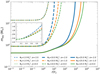 |
Fig. 5 Theoretical radial profile of the equipartition mass obtained for different values of the model parameters Φ0 (same line style) and α(same colors and line width). The panel zooms onto the core region r ≤ rc. |
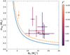 |
Fig. 6 Equipartition mass meq in the core (r ≤ rc) as function of Φ0. The blue continuous line and the orange dashed line are the 3D and 2D theoretical predictions, respectively. The circles with error bars are the same as in Fig. 2. |
3.4 Relation with structural parameters
The dynamical state of GCs is related to the amount of relaxation they experienced during their life. A dynamically old cluster has seen several relaxation timescales trelax during its evolution, a time that is shorter in the central regions, being gravitational interactions more frequent. In literature, the relaxation process is often quantified with the relaxation timescale in the core trc (Djorgovski 1993) and at half-mass radius (Binney & Tremaine 2008), which have an analytical approximated formula for their evaluation. This leads W22 to compare their prediction of meq with the number of core and median relaxation timescales Ncore and Nhalf, as shown in their Fig. 16.
From the King (1966) model, it is also expected that dynamically evolved clusters have a greater concentration c = log(rt/rk) value, with the King radius rk often replaced with the core radius rc . Indeed, a monotonically increasing relation exists between the concentration and the corresponding W0 equilibrium parameter of the King model.
In the framework of our multi-mass dynamical model, the equilibrium configuration is identified by Φ0 . However, the scaling radius of the model rk,u loses, in principle, the relation with the core radius that the King model had. This leads us to define the equivalent King concentration ck = log(rt/ rk,u) and the theoretical concentration cth = log(rt/rc,th), with rc,th estimated from the surface density profile, assuming a proportionality relationship between the mass and luminosity density profiles (as outlined before). These concentrations have a small relative difference and both monotonically increase with Φ0, following a trend that depends on the slope α. In the perspective of comparing with observations, we consider only cth.
About the relaxation timescale, the model derivation highlights a dependence on mass, consistent with what is observed. However, obtaining an analytical formula requires further investigation and development. We are then limited to take the values of Ncore and Nhalf from literature.
We expect that Φ0 increases with Ncore, Nhalf and cobs = log(rt/rc). For the core and median relaxation timescales numbers we take the same values considered by W22, while for the concentrations we consider c in the Harris catalog and its estimation obtained with two sources for the core radius, the one in the Harris catalog and the other by Baumgardt (2018–2023) online catalog (which used the Spitzer 1987 definition), while for the tidal radius we refer to Webb et al. (2013), reported in the same catalog.
In Fig. 7, the previously estimated values of Φ0 are given with the concentration. We show the theoretical relation for some choices of the slope α, against the observational concentrations from different sources. The predicted concentration grows continuously with Φ0, as already stated, but there are differences with the observational ones. From the model point of view, such discrepancy can be related to the fit quality and the value of the theoretical core radius. Low fit quality results can give an incorrect estimate of Φ0, which affects the vertical positions of each marker in the pictures. Concerning the core radius, the adopted choice is reasonable, since it is based on the assumption that the luminosity density profile is proportional to the density profile, with a multiplying factor only dependent on mass. From the observational point of view, we first note that the Harris catalog concentrations come by fitting the surface brightness profile of clusters with a King single-mass model (King 1966), which has been found to be in disagreement with observations in the outer regions, being clusters more extended, like already pointed out so far by Da Costa & Freeman (1976). Indeed, the authors found that the outer regions of M3 can be described by a King profile with c = 1.98, while the inner ones using c = 1.29. This suggests that clusters are more extended and, consequently, have a higher concentration with respect to the single-mass model prediction. Multi-mass models can overcome such discrepancy, being more extended. In principle, a concentration value completely based on observations requires the knowledge of both the core radius and the tidal radius. While the first is easier to measure, the latter is quite tricky, since a clear distinction between stars that belong to the cluster or are leaving it is difficult to infer. This leads us to compute the concentration using the core and tidal radius from different sources (Baumgardt 2018–2023; Harris 1996; Webb et al. 2013). Indeed, Webb et al. (2013) found an empirical formula for the limiting radius of GCs through N-body simulations, which takes the orbital properties of the system in the galactic gravitational potential into account. This results in a greater tidal radius and consequently a greater concentration with respect to the King ones from the Harris catalog, as can be inferred from Fig. 7, comparing the orange squares and the green stars with the blue triangles. Such tendency slightly erases the differences with the theoretical prediction, with the only exception of NGC 5139 (ω-Cen), which however is a complex object, as already mentioned, whose deviation is not so surprising.
Our analysis of few clusters reveals that there are important inhomogeneities among observational-based concentrations. Indeed, we can state that the estimate of the concentration suffers several sources of errors that can differ between clusters. The difficulty of measuring the tidal radius and, consequently, the concentration suggests to recover the role of theoretical models in predicting its value, as it was for the King model. The concentration value could be estimated from the relationship with the gravitational potential well through Φ0, to be constrained fitting observational profiles with model predictions. Anyway, an extensive comparison between the theoretically predicted concentrations and the observational ones must be addressed in future works, with a greater GCs sample and heterogeneous observational sources.
In Fig. 8, we show the relation between the gravitational potential and the number of core and median relaxation timescales. The plot shows a tendency of having greater Φ0 values with a larger Ncore and Nhalf , as expected for more dynamically evolved states. A similar trend was found by W22 with the meq parameter. Unfortunately, the great errors and the absence of a theoretical prediction on Ncore and Nhalf do not allow us to further discuss the obtained pattern.
Another quantifier of the dynamical state of GCs is the so-called dynamical-clock, mainly measured through the A+ parameter that is the area between the cumulative distribution of Blue Straggler Stars (BSSs) and the reference stars (Ferraro et al. 2012, 2020; Alessandrini et al. 2016; Lanzoni et al. 2016). Only four of the analyzed GCs have a measure of A+, which also well correlates with the number of core relaxation timescales and the core radius, as shown by Lanzoni et al. (2016) and Ferraro et al. (2018). We give in Fig. 9 the estimated Φ0 and the corresponding A+ and log(rc), where we use again the core radius from the Harris catalog and Baumgardt (2018–2023) online catalog.
As for the number of core relaxation timescales, the Φ0 parameter grows at increasing values of A+, both measuring the dynamical state of GCs, although the number of points is small and only a general increasing trend can be deduced. While Φ0 measures the gravitational potential well, the A+ parameter tracks the segregation of BSSs with respect to the other stars, measuring the mass segregation process. They have a lower velocity dispersion value, corresponding to their expected higher mass with respect to reference stars, namely the main sequence turn-off mass (see Baldwin et al. 2016, and references therein). In principle, the mass of BSSs depends on the formation mechanisms of such objects, which is still unknown. The most spread idea is that they are binary stars or a result of stellar coalescence. To precisely measure the dynamical state of the cluster, the formation of such objects should be mostly coeval with the cluster itself. Any recently formed BSS will naturally be less segregated, meaning that the overall BSSs population segregation will decrease, resulting in a lower dynamical state for the cluster. Indeed, the dynamical processes that bring the collisional system toward mass segregation and energy equipartition are phenomena that strongly depend on the mass of the object and the relation between its age and the relaxation timescale. Our work, as well as several energy equipartition studies in literature, underlines that massive stars are faster in reaching equipartition than less massive ones. Consequently, the population of BSSs can have internal differences in their kinematic properties if a spread in mass exists. As we observe and predict a different degree of energy equipartition for reference stars, a similar phenomenology can state also for BSSs. One of the main strength of our modeling approach is the ability of predicting such kinematic differences for objects with whatever mass, once known their mass function and the structural parameter Φ0. That would further broaden the role of BSSs in characterizing GCs dynamical state and understanding the complex internal dynamics, giving important insight in the energy equipartition and mass segregation topics.
Concerning the relation with the core radius, advanced dynamical states have a greater value of Φ0 and a lower rc, as shown in the lower panel of Fig. 9, which also affects the concentration that will be higher. Indeed, as the relaxation proceed, the cluster is driven toward the core collapse phase and the gravothermal catastrophe. Here, the structure of the system is altered and King-based models do not reproduce well the structural properties. However, the energy equipartition keeps going on in the survived core, where a higher degree of equipartition can be expected. As mentioned in Sect. 3.1, the estimates of Φ0 from the observable σ(m) may suffer from a systematic effect related to the adopted value for the core radius, which is neglected in our analysis. With simple order-of-magnitude calculations and a linear interpolation of the Φ0−log (rc) relation, in the case of NGC 5904 and NGC 6397 a 10% variation in the core radius is requested to get a systematic shift on Φ0 comparable to the estimated statistical error. For all the other clusters in our sample, the variation of rc should be much larger. Although the relative error for the core radius is typically smaller, as can be seen from Table 4, larger discrepancies are found when the Harris catalog values are compared to those of Baumgardt (2018–2023).
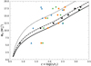 |
Fig. 7 Relation between Φ0 and the concentration c = log(rt/rc). The continuous, dashed, and dotted lines represent, respectively, the theoretical prediction with a mass function slope α = 0.0, α = −1.0, and α = −2.0, while the black circles show the constrained values of Φ0 and c for the analyzed clusters. The blue triangles show the King concentration from the Harris (1996) catalog (2010 edition), while the orange squares and green stars are computed using the core radius from the Harris (1996) and Baumgardt (2018–2023) catalogs respectively, and the tidal radius from Webb et al. (2013). |
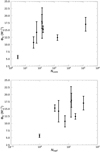 |
Fig. 8 Obtained values of Φ0 against the number of core relaxation timescales Ncore (upper panel) and the number of median relaxation timescales Nhalf (lower panel) from Watkins et al. (2022). |
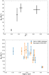 |
Fig. 9 Comparison of structural parameters that measure the dynamical state of globular clusters. Upper panel: relation between Φ0 and the area A+ between the cumulative distribution of blue straggler stars and the reference stars. Lower panel: Φ0 relation with the core radius, using values from the Harris (1996) catalog (blue triangles) and the Baumgardt (2018–2023) online catalog (orange squares). |
Structural parameters obtained by fitting SBPs.
3.5 Fitting surface brightness profiles
To provide an independent determination of the structural parameter Φ0, we fit the SBPs data by Trager et al. (1995) with the prediction of the dynamical model, by using theoretical isochrones from BaSTI (Hidalgo et al. 2018; Pietrinferni et al. 2021; Salaris et al. 2022; Pietrinferni et al. 2024) for an age of 13 Gyrs, with [α/Fe] = +0.4, Y = 0.247 and a different metal- licity [Fe/H] for each cluster, taken from the Harris catalog, as described in Sect. 2.2.2.
In Fig. 10, we plot the obtained best-fit profile for NGC 6341. In Table 4, we give the estimated Φ0 as well as the central surface brightness, the core and tidal radius and the normalized χ2 value for the analyzed clusters.
The obtained best-fit curves reproduce well the observed data, with a very narrow error band and small uncertainties for the parameters. However, the obtained estimates neglect possible error sources, both statistical and systematic ones. Regarding the conversion of the observed magnitudes into luminosities, several systematic effects can occur, as due to the extinction values or the distance modulus value as well as in the assumed solar V- magnitude. However, all these parameters produce an offset in the magnitude, but they do not affect our minimization procedure and the obtained Φ0. This is not the case for the parameters related to the isochrones, such as the age and the adopted values of [α/Fe], He abundance and [Fe/H]. As an example, we report in the last column of Table 4 the effect of a different age in the estimated value of Φ0, using isochrones at 11 Gyr, keeping the previous adopted values for [α/Fe], Y and [Fe/H]. The overall impact of a reduced age is a smaller Φ0 , resulting in a systematic effect. As already explained in Sect. 2.2.2, a smaller age implies a larger maximum mass. Since more massive stars are more segregated and affect the luminosity distribution in the innermost region of the cluster, a steeper brightness profile is expected. Therefore, in order to reproduce the observed SBP, the effect of an increase in the maximum mass should be compensated by a reduction of the Φ0 value. We note that we cannot distinguish from the 11 Gyr and 13 Gyr cases, because the implied variations of the observable parameters (such as the central surface brightness, core radius and tidal radius) are smaller than their respective statistical errors. In addition, the isochrones vary from cluster to cluster also due to the different metallic- ity that we considered. The role of the metallicity, [α/Fe], He mass fraction Y, and cluster age in shaping GCs SBPs, especially in the framework of multi-mass King-like models, requires a broader exploration and a dedicated work. The same holds for the mass function shape, which can alter the predictions due to its structural role, being a fundamental physical ingredient in such dynamical models. In fact, the massive stars content is extremely important in shaping the SBPs and thus the slope α is expected to play a relevant effect.
Finally, we compare the independent estimates of Φ0 obtained from internal kinematics, namely the velocity dispersion as function of stellar mass, with those from the SBPs. Concerning the latter, we first account for age variations by averaging the corresponding Φ0 values and computing the associated uncertainty. In Fig. 11, we plot the relative variation ΔΦ0/〈Φ0〉, showing the 2σ confidence interval. The two estimates are compatible at 2σ level for most clusters, although some are compatible at 1σ confidence interval (namely NGC 5904, NGC 6266 and NGC 6656). The larger deviation is obtained for NGC 5139 (ω-Cen). As already mentioned, this cluster is a much more complex object. It is probably the remnant of a dwarf galaxy. It hosts multiple stellar generations, also showing metallicity variations, for which multiple isochrones should be used and potentially multiple dynamical states for each of the subsystems that make up such an object.
The plot also highlights how multi-mass King-like dynamical models can predict both internal kinematics and the surface brightness profiles. However, as already outlined, there are several possible sources of error that could further increase our uncertainties in the Φ0 estimates. A full exploration of the assumptions made in the SBPs fitting procedure is needed to better constrain the Φ0 value. Only afterward, its relation with the other structural quantities such as concentration, number of relaxation times, core radius and A+ can be addressed similarly to what done in Sect. 3.4.
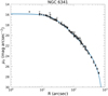 |
Fig. 10 Surface brightness profile for NGC 6341. The black circles with error bars are the data from Trager et al. (1995) analyzed following the work by McLaughlin & van der Marel (2005) and Zocchi et al. (2012). The continuous blue line is our model best fit with its confidence band, which is obtained by assuming the Baumgardt et al. (2023) mass function slope and adopting the BaSTI isochrones (Hidalgo et al. 2018; Pietrinferni et al. 2021; Salaris et al. 2022; Pietrinferni et al. 2024) with 13 Gyr, [α/Fe] = +0.4, Y = 0.247, and metallicity [Fe/H]=−2.31, taken from the Harris (1996) catalog (2010 edition). |
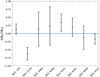 |
Fig. 11 Relative variation in the estimates of the Φ0 parameter for each of the analyzed clusters, obtained by fitting the velocity dispersion dependence on stellar mass σ(m) and the surface brightness profiles I(R). The error bars are the 2σ level uncertainties. |
4 Conclusions
In this work, we explore the degree of energy equipartition in GCs by means of a multi-mass King-like dynamical model for collisional and phase-space-limited systems. This theoretical description offers an efficient way to predict several dynamical processes occurring in GCs, such as energy equipartition, mass segregation, and evaporation. These phenomena alter the properties of clusters, modifying their spatial and kinematic structure. Here we focus on the degree of equipartition, and determine the dynamical state of a few GCs by means of model parameters.
We fit the velocity dispersion dependence on the stellar mass – measured through HST proper motions by Watkins et al. (2022) – with our prediction, discussing the relation with the Bianchini et al. (2016) fitting function and the equipartition mass meq. We obtain a similar confidence level and a relation between the equipartition mass and the model parameter Φ0 , which is a measure of the gravitational potential difference between the center and the edge of the cluster. An increasing value for this quantity describes a more dynamically old cluster, with a larger degree of energy equipartition, which is in turn associated with a lower value of meq.
We confirm that the energy equipartition in the analyzed GCs is only partial, even in the central regions. The equipartition degree appears similar in the core, while decreasing significantly in the outer regions. More massive stars are closer to equipartition than less massive ones, as already found and outlined in other works.
We extend our fitting procedure by adding the slope of the mass function α to the parameter space; α is a required input for the model, and we take its value from Baumgardt et al. (2023). This procedure provides similar results regarding the estimate of Φ0 , but prevents any constraint on the mass function slope using the data. Although we obtain a degeneration between the two parameters, the effect of varying the gravitational potential well alters the observable σ(m) to a greater degree than the variations in the mass function when reasonable (i.e., α є [−2.0, 0]).
We carefully discuss the implications of quantifying the degree of energy equipartition through the Bianchini fitting function with respect to our dynamical model prediction, when working with a restricted radial shell and projected quantities. We find that the estimated meq from the projected dispersion is higher than the three-dimensional one. Moreover, for radial shells overcoming the core radius, the equipartition mass underestimates the maximum degree of equipartition reached in the core. On the contrary, the equilibrium parameter Φ0 uniquely defines both projected and 3D radial theoretical profiles, without suffering shell selection or projection effects. We also find that variations in the slope α affect the degree of equipartition mainly in the outer regions, while their effect is relatively small in the core. Here, by fitting theoretical profiles with the Bianchini function, we obtain a mostly constant meq, suggesting that this value can be used as a measure of the maximum degree of energy equipartition in clusters. However, taking advantages of dynamical models like ours offers the opportunity to quantify the degree of equipartition in the cores of clusters by means of structural parameters. Here, observational data suffer several limitations and a theoretical tool for predicting observables can offer important support to the astronomical community.
We compare the estimates of Φ0 with other structural properties of GCs that depend on the dynamical state of the system. The theoretical relation between Φ0 and the concentration is presented, as is the relation between the estimated Φ0 and observational values for the concentration from different sources (Harris 1996; Baumgardt 2018–2023; Webb et al. 2013). The spread among observations as well as the differences with respect to the theoretical prediction highlight the presence of several sources of error. However, the theoretical relation between Φ0 and the concentration provides an important tool to constrain the latter on a more fundamental ground, once the former is properly estimated. Consequently, we advise to recover the predicting role of models concerning the determination of the concentration value for GCs. A positive trend is also seen between Φ0 and the number of core and median relaxation timescales. We note a similar trend for the area A+ between the cumulative distributions of blue straggler stars and reference stars (Lanzoni et al. 2016; Ferraro et al. 2018), although the number of points is small (only four clusters). All such structural quantities, such as Φ0 , increase for dynamically old systems. Conversely, the core radius decreases with the dynamical state, a trend we clearly see between Φ0 and rc. These outcomes strongly suggest that we can include Φ0 among the properties that track the dynamical age of GCs. However, a statistically robust comparison between the structural parameters of Galactic GCs and those of our model must be carried out in future works, with a wider sample of clusters.
Finally, we successfully fit the surface brightness profiles by Trager et al. (1995) following a procedure similar to that described by Trenti & van der Marel (2013) and Zocchi et al. (2012). To make the theoretical prediction, we need the surface density profile and a mass–luminosity relation, which we take from theoretical isochrones (Hidalgo et al. 2018; Pietrinferni et al. 2021; Salaris et al. 2022; Pietrinferni et al. 2024). We obtain an estimate for Φ0 , the central surface brightness, the core, and the tidal radius. We discuss the possible effects that can alter our predictions, mainly in regard to the mass–luminosity relation. A different age for the isochrone introduces a systematic error in the determination of Φ0 that is larger than the statistical uncertainty inherent to the fitting procedure. We average these contributions to get Φ0 estimates from the fitting procedure on each cluster SBP. We compare these values with the ones computed by fitting the velocity dispersion–mass relation, showing that they are compatible at the 2σ level for almost all clusters. The largest deviation is obtained for ω-Cen, whose complexity suggests that our fitting procedure needs to be extended to consider multiple stellar populations with different chemical contents and metallicities, and consequently different isochrones.
The obtained results strongly underline the central role of dynamical models in predicting the phenomenology of GCs, such as the highly debated energy equipartition process. With the increasing amount of information coming from internal kinematics observations, more effort must be put into advanced physical modeling. Such models are powerful tools for elucidating the mechanisms behind several dynamical phenomena, such as segregation and evaporation, as well as anisotropic velocity distributions and internal rotation. However, determinations of the dynamical state and predictions of the different observables are affected by several sources of error. These errors are related to, for example, the internal kinematics and the surface brightness profiles, where the role of the assumptions made regarding structural properties and the mass–luminosity relation must be further explored.
Data availability
Appendix B is available on Zenodo.
Acknowledgements
MT thanks Michele Bellanzini for important hints that expanded this work. The authors would thank the anonymous referee for the useful indications and comments that improved this paper.
Appendix A Model derivation
The distribution function (DF) that defines our model is given in Eq. (2). It comes from an analytical derivation, which replicates and adapt the analytical procedures that brought from the dynamical friction (Chandrasekhar 1943) to the King (1966) model. In King (1965), the author obtained a DF as an approximated solution of the Fokker-Planck equation, valid for collisional systems. Then, he generalized and used it in King (1966). Our DF keeps the memory of the King one, but takes the mass distribution into account, as was done by Da Costa & Freeman (1976). They presented a discrete model, where each mass class has a DF with an energy cut-off and a weight factor, to be constrained from observations. In principle, the assumption that each mass has that specific DF analytical shape must be proved similarly, solving the Fokker-Planck equation in a multi-mass system.
The procedure that lead to the King DF starts from the Boltzmann equation for collisional systems and follows the Chandrasekhar (1943) development: assuming local approximation and low energy exchanges, the equation is written in terms of the diffusion coefficients, which quantify the dynamical friction that a test star with mass m suffers due to field stars with mass ma. Following Binney & Tremaine (2008), the Spitzer & Härm (1958) expression of the Fokker-Planck equation is obtained. King was able to solve such equation in 1965 with an approximation. He originally obtained a DF where both masses m and ma appear, but then he takes them equal.
In principle, the same approach can be followed again, but taking care of considering the field stars’ mass function when evaluating the diffusion coefficients, as well as their velocity distribution, assumed Maxwell-Boltzmann like. A further needed step is the distinction between dynamical quantities and thermodynamic ones. In particular, when using a Maxwell-Boltzmann DF for field stars, which is ![Mathematical equation: $ \propto \exp \left[ { - {v^2}/\left( {2\sigma _{\rm{a}}^2} \right)} \right]$](/articles/aa/full_html/2024/11/aa50783-24/aa50783-24-eq35.png) , one gets the scaling factor σa which is related to the thermodynamic temperature θ (kept constant) and the field stars’ mass, namely
, one gets the scaling factor σa which is related to the thermodynamic temperature θ (kept constant) and the field stars’ mass, namely  . In this framework σ is the 1D velocity dispersion of the Maxwell-Boltzmann DF, and it depends only on the mass, while there is another quantity that comes at the end of the procedure, namely the kinetic one. In the limit of a Maxwell-Boltzmann DF for the test star (that describes an isothermal sphere) the kinetic quantity converges to the thermodynamic one. This distinction allows us to explicit mass dependence in the obtained generalized expression of the Fokker-Planck equation, which finally states
![Mathematical equation: ${{{\rm{d}}f} \over {{\rm{d}}t}} = {1 \over {{t_{\rm{R}}}(m)}}{1 \over {{x^2}}}{\partial \over {\partial x}}\left[ {2x{\cal G}(x,m)\left( {2xf + {{\partial f} \over {\partial x}}} \right)} \right],$](/articles/aa/full_html/2024/11/aa50783-24/aa50783-24-eq37.png) (A.1)
(A.1)
where f = f (x, m; t) is the DF of the test star, x = v2/(2σ2) and
![Mathematical equation: ${{{\cal G}(x,m)} \over {{t_{\rm{R}}}(m)}} = \int_{\Delta {m_{\rm{a}}}} {{1 \over {{\tau _{{\rm{R}},{\rm{a}}}}}}} {\left( {{m \over {{m_{\rm{a}}}}}} \right)^{3/2}}\left[ {{2 \over {\sqrt \pi x_{\rm{a}}^2}}\int_0^{{x_{\rm{a}}}} {{y^2}} {{\rm{e}}^{ - {y^2}}}{\rm{d}}y} \right]{\rm{d}}{m_{\rm{a}}},$](/articles/aa/full_html/2024/11/aa50783-24/aa50783-24-eq38.png) (A.2)
(A.2)
with  the relaxation time for binary encounters between m and ma , with the latter distributed in the interval Δma. Here, tR(m) is the relaxation time of the mass m, due to gravitational encounters with all the field stars.
Following King (1965), Eq. (A.1) can be solved similarly assuming f (x, m; t) = ց(x, m)exp[−λ(m) t/1R(m)], with λ the evaporation rate of stars with mass m and ց(x, m) = A(m)ḡ(x, m), which brings the dependence on x and the dimensions in the multiplying factor A(m). With an expansion in power series of the evaporation rate, with boundary conditions ḡ(0) = 1, ḡ′(0) = 0 and ḡ(xe) = 0 where xe is the cut-off, we obtain the approximated solution for ց(x, m) in the central region, where the treatment is valid, that is
![Mathematical equation: $g(x,m) = k(m)\left[ {\exp \left( { - {x^2}} \right) - \exp \left( { - x_{\rm{e}}^2} \right)} \right],$](/articles/aa/full_html/2024/11/aa50783-24/aa50783-24-eq40.png) (A.3)
(A.3)
with k(m) that gathers all the mass-dependent multiplying factors. From the reasonable assumption that field stars have a Maxwell-Boltzmann DF, to be recovered in the limit of an infinite escape velocity (i.e., the isothermal sphere), and since the DFs we are dealing with give the number of stars in the infinitesimal volume d3v d3 r dm, it results that
![Mathematical equation: $k(m) = {\left( {{m \over {2\pi {k_{\rm{B}}}\theta }}} \right)^{3/2}}{{{\rm{d}}{n_0}(m)} \over {{\rm{d}}m}}{\left[ {1 - \exp \left( { - x_{\rm{e}}^2} \right)} \right]^{ - 1}},$](/articles/aa/full_html/2024/11/aa50783-24/aa50783-24-eq41.png) (A.4)
(A.4)
where n0(m) is the number density of stars with mass between m and m + dm in the central region and dn0/dm = ξ0(m)/ V with ξ0(m) the mass function and V the volume of the central region.
The final step is the generalization to different radial regions. Applying the Jeans theorem leads to the DF in Eq. (2) that is given in terms of the kinetic energy and cut-off energy.
References
- Alessandrini, E., Lanzoni, B., Ferraro, F. R., Miocchi, P., & Vesperini, E. 2016, ApJ, 833, 252 [NASA ADS] [CrossRef] [Google Scholar]
- Ambartsumyan, V. A. 1938, Trudy Astron. Obs. Leningr. Gos. Univ., 7, 19 [Google Scholar]
- Aros, F. I., & Vesperini, E. 2023, MNRAS, 525, 3136 [NASA ADS] [CrossRef] [Google Scholar]
- Baldwin, A. T., Watkins, L. L., van der Marel, R. P., et al. 2016, ApJ, 827, 12 [NASA ADS] [CrossRef] [Google Scholar]
- Bastian, N., & Lardo, C. 2018, ARA&A, 56, 83 [Google Scholar]
- Baumgardt, H. 2018-2023, Structural Parameters of Galactic Globular Clusters, website [Google Scholar]
- Baumgardt, H., Hénault-Brunet, V., Dickson, N., & Sollima, A. 2023, MNRAS, 521, 3991 [CrossRef] [Google Scholar]
- Bianchini, P., van de Ven, G., Norris, M. A., Schinnerer, E., & Varri, A. L. 2016, MNRAS, 458, 3644 [NASA ADS] [CrossRef] [Google Scholar]
- Bianchini, P., Webb, J. J., Sills, A., & Vesperini, E. 2018, MNRAS, 475, L96 [CrossRef] [Google Scholar]
- Binney, J., & Tremaine, S. 2008, Galactic Dynamics (Princeton University Press) [Google Scholar]
- Chandrasekhar, S. 1943, ApJ, 97, 255 [Google Scholar]
- Chandrasekhar, S. 1943, Rev. Mod. Phys., 15, 1 [CrossRef] [Google Scholar]
- Chandrasekhar, S. 1960, Principles of Stellar Dynamics (New York: Dover Pubblications, Inc.) [Google Scholar]
- Da Costa, G. S., & Freeman, K. C. 1976, ApJ, 206, 128 [NASA ADS] [CrossRef] [Google Scholar]
- Dickson, N., Hénault-Brunet, V., Baumgardt, H., Gieles, M., & Smith, P. J. 2023, MNRAS, 522, 5320 [NASA ADS] [CrossRef] [Google Scholar]
- Djorgovski, S. G., & Meylan, G. 1993, Structure and Dynamics of Globular Clusters (ASP Conf. Ser. Vol. 50 Astron. Soc. Pac.) [Google Scholar]
- Ferraro, F. R., Lanzoni, B., Dalessandro, E., et al. 2012, Nature, 492, 393 [Google Scholar]
- Ferraro, F. R., Lanzoni, B., Raso, S., et al. 2018, ApJ, 860, 36 [NASA ADS] [CrossRef] [Google Scholar]
- Ferraro, F. R., Lanzoni, B., & Dalessandro, E. 2020, Rend. Lincei. Sci. Fis. Natur., 31, 19 [CrossRef] [Google Scholar]
- Gieles, M., & Zocchi, A. 2015, MNRAS, 454, 576 [NASA ADS] [CrossRef] [Google Scholar]
- Gratton, R., Bragaglia, A., Carretta, E., et al. 2019, A&A Rev., 27, 8 [NASA ADS] [CrossRef] [Google Scholar]
- Harris, W. E. 1996, AJ, 112, 1487 [Google Scholar]
- Hidalgo, S. L., Pietrinferni, A., Cassisi, S., et al. 2018, ApJ, 856, 125 [Google Scholar]
- King, I. 1958a, AJ, 63, 109 [NASA ADS] [CrossRef] [Google Scholar]
- King, I. 1958b, AJ, 63, 114 [NASA ADS] [CrossRef] [Google Scholar]
- King, I. R. 1965, AJ, 70, 376 [NASA ADS] [CrossRef] [Google Scholar]
- King, I. R. 1966, AJ, 71, 64 [Google Scholar]
- Lanzoni, B., Ferraro, F. R., Alessandrini, E., et al. 2016, ApJ, 833, L29 [NASA ADS] [CrossRef] [Google Scholar]
- Libralato, M., Bellini, A., van der Marel, R. P., et al. 2018, ApJ, 861, 99 [CrossRef] [Google Scholar]
- Libralato, M., Bellini, A., Piotto, G., et al. 2019, ApJ, 873, 109 [NASA ADS] [CrossRef] [Google Scholar]
- Libralato, M., Bellini, A., Vesperini, E., et al. 2022, ApJ, 934, 150 [NASA ADS] [CrossRef] [Google Scholar]
- McLaughlin, D. E., & van der Marel, R. P. 2005, ApJS, 161, 304 [NASA ADS] [CrossRef] [Google Scholar]
- Merafina, M. 2017, Int. J. Mod. Phys. D, 26, 1730017 [NASA ADS] [CrossRef] [Google Scholar]
- Merafina, M. 2018, in Proceedings of XII Multifrequency Behaviour of High Energy Cosmic Sources Workshop — PoS(MULTIF2017), 306, 004 [CrossRef] [Google Scholar]
- Merafina, M. 2019, in Proceedings of Frontier Research in Astrophysics III — PoS(FRAPWS2018), 331, 010 [CrossRef] [Google Scholar]
- Milone, A. P., & Marino, A. F. 2022, Universe, 8, 359 [NASA ADS] [CrossRef] [Google Scholar]
- Miocchi, P. 2006, MNRAS, 366, 227 [NASA ADS] [CrossRef] [Google Scholar]
- Miocchi, P., Lanzoni, B., Ferraro, F. R., et al. 2013, ApJ, 774, 151 [Google Scholar]
- Noyola, E., & Gebhardt, K. 2006, AJ, 132, 447 [Google Scholar]
- Odenkirchen, M., Grebel, E. K., Rockosi, C. M., et al. 2001, ApJ, 548, L165 [Google Scholar]
- Pavlík, V., & Vesperini, E. 2021a, MNRAS, 509, 3815 [CrossRef] [Google Scholar]
- Pavlík, V., & Vesperini, E. 2021b, MNRAS, 504, L12 [CrossRef] [Google Scholar]
- Pavlík, V., & Vesperini, E. 2022, MNRAS, 515, 1830 [CrossRef] [Google Scholar]
- Peterson, C. J., & King, I. R. 1975, AJ, 80, 427 [NASA ADS] [CrossRef] [Google Scholar]
- Peuten, M., Zocchi, A., Gieles, M., & Hénault-Brunet, V. 2017, MNRAS, 470, 2736 [CrossRef] [Google Scholar]
- Piatti, A. E., & Carballo-Bello, J. A. 2020, A&A, 637, L2 [NASA ADS] [CrossRef] [EDP Sciences] [Google Scholar]
- Pietrinferni, A., Hidalgo, S., Cassisi, S., et al. 2021, ApJ, 908, 102 [NASA ADS] [CrossRef] [Google Scholar]
- Pietrinferni, A., Salaris, M., Cassisi, S., et al. 2024, MNRAS, 527, 2065 [Google Scholar]
- Rosenbluth, M. N., MacDonald, W. M., & Judd, D. L. 1957, Phys. Rev., 107, 1 [NASA ADS] [CrossRef] [Google Scholar]
- Salaris, M., Cassisi, S., Pietrinferni, A., & Hidalgo, S. 2022, MNRAS, 509, 5197 [Google Scholar]
- Spitzer, L. 1987, Dynamical Evolution of Globular Clusters (Princeton University Press) [Google Scholar]
- Spitzer, L., & Härm, R. 1958, ApJ, 127, 544 [NASA ADS] [CrossRef] [Google Scholar]
- Torniamenti, S., Bertin, G., & Bianchini, P. 2019, A&A, 632, A67 [NASA ADS] [CrossRef] [EDP Sciences] [Google Scholar]
- Torres, G. 2010, AJ, 140, 1158 [Google Scholar]
- Trager, S. C., King, I. R., & Djorgovski, S. 1995, AJ, 109, 218 [NASA ADS] [CrossRef] [Google Scholar]
- Trenti, M., & van der Marel, R. 2013, MNRAS, 435, 3272 [NASA ADS] [CrossRef] [Google Scholar]
- Vesperini, E., Hong, J., Giersz, M., & Hypki, A. 2021, MNRAS, 502, 4290 [NASA ADS] [CrossRef] [Google Scholar]
- von Hoerner, S. 1957, ApJ, 125, 451 [NASA ADS] [CrossRef] [Google Scholar]
- Wang, L., Spurzem, R., Aarseth, S., et al. 2016, MNRAS, 458, 1450 [Google Scholar]
- Watkins, L. L., van der Marel, R. P., Libralato, M., et al. 2022, ApJ, 936, 154 [CrossRef] [Google Scholar]
- Webb, J. J., & Vesperini, E. 2017, MNRAS, 464, 1977 [NASA ADS] [CrossRef] [Google Scholar]
- Webb, J. J., Harris, W. E., Sills, A., & Hurley, J. R. 2013, ApJ, 764, 124 [Google Scholar]
- Webb, J. J., Reina-Campos, M., & Kruijssen, J. M. D. 2019, MNRAS, 486, 5879 [NASA ADS] [CrossRef] [Google Scholar]
- Zocchi, A., Bertin, G., & Varri, A. L. 2012, A&A, 539, A65 [NASA ADS] [CrossRef] [EDP Sciences] [Google Scholar]
All Tables
All Figures
|
Fig. 1 Projected velocity dispersion as a function of stellar mass for NGC 6397. The error bars are the data from Watkins et al. (2022), the continuous green line is our best fit with the Bianchini et al. (2016) fitting function in Eq. (1) with its error band, the dotted brown line is the complete equipartition limit (σ ∝ m−1/2), and the dashed orange line is our model best-fit with its 68% confidence band. |
| In the text | |
|
Fig. 2 Relation between the estimated Φ0 and meq from Watkins et al. (2022). The χ2 test value is given by the color of the data point for each NGC according to the color bar to the right. |
| In the text | |
|
Fig. 3 Contour plot for NGC 6397 in the Φ0−α plane, showing the χ2 levels. The blue band gives the slope from Baumgardt et al. (2023). Squares indicate the χ2 values around the minimum, which is identified by a large gray circle. |
| In the text | |
|
Fig. 4 Radial and projected profile of the equipartition mass meq, obtained by fitting the model prediction of the velocity dispersion with the Bianchini function at each radial coordinate, given in units of the core radius. The panel zooms onto the region r ≤ rc. |
| In the text | |
|
Fig. 5 Theoretical radial profile of the equipartition mass obtained for different values of the model parameters Φ0 (same line style) and α(same colors and line width). The panel zooms onto the core region r ≤ rc. |
| In the text | |
|
Fig. 6 Equipartition mass meq in the core (r ≤ rc) as function of Φ0. The blue continuous line and the orange dashed line are the 3D and 2D theoretical predictions, respectively. The circles with error bars are the same as in Fig. 2. |
| In the text | |
|
Fig. 7 Relation between Φ0 and the concentration c = log(rt/rc). The continuous, dashed, and dotted lines represent, respectively, the theoretical prediction with a mass function slope α = 0.0, α = −1.0, and α = −2.0, while the black circles show the constrained values of Φ0 and c for the analyzed clusters. The blue triangles show the King concentration from the Harris (1996) catalog (2010 edition), while the orange squares and green stars are computed using the core radius from the Harris (1996) and Baumgardt (2018–2023) catalogs respectively, and the tidal radius from Webb et al. (2013). |
| In the text | |
|
Fig. 8 Obtained values of Φ0 against the number of core relaxation timescales Ncore (upper panel) and the number of median relaxation timescales Nhalf (lower panel) from Watkins et al. (2022). |
| In the text | |
|
Fig. 9 Comparison of structural parameters that measure the dynamical state of globular clusters. Upper panel: relation between Φ0 and the area A+ between the cumulative distribution of blue straggler stars and the reference stars. Lower panel: Φ0 relation with the core radius, using values from the Harris (1996) catalog (blue triangles) and the Baumgardt (2018–2023) online catalog (orange squares). |
| In the text | |
|
Fig. 10 Surface brightness profile for NGC 6341. The black circles with error bars are the data from Trager et al. (1995) analyzed following the work by McLaughlin & van der Marel (2005) and Zocchi et al. (2012). The continuous blue line is our model best fit with its confidence band, which is obtained by assuming the Baumgardt et al. (2023) mass function slope and adopting the BaSTI isochrones (Hidalgo et al. 2018; Pietrinferni et al. 2021; Salaris et al. 2022; Pietrinferni et al. 2024) with 13 Gyr, [α/Fe] = +0.4, Y = 0.247, and metallicity [Fe/H]=−2.31, taken from the Harris (1996) catalog (2010 edition). |
| In the text | |
|
Fig. 11 Relative variation in the estimates of the Φ0 parameter for each of the analyzed clusters, obtained by fitting the velocity dispersion dependence on stellar mass σ(m) and the surface brightness profiles I(R). The error bars are the 2σ level uncertainties. |
| In the text | |
Current usage metrics show cumulative count of Article Views (full-text article views including HTML views, PDF and ePub downloads, according to the available data) and Abstracts Views on Vision4Press platform.
Data correspond to usage on the plateform after 2015. The current usage metrics is available 48-96 hours after online publication and is updated daily on week days.
Initial download of the metrics may take a while.