| Issue |
A&A
Volume 695, March 2025
|
|
|---|---|---|
| Article Number | A216 | |
| Number of page(s) | 20 | |
| Section | Cosmology (including clusters of galaxies) | |
| DOI | https://doi.org/10.1051/0004-6361/202449599 | |
| Published online | 20 March 2025 | |
The SRG/eROSITA All-Sky Survey
Weak lensing of eRASS1 galaxy clusters in KiDS-1000 and consistency checks with DES Y3 and HSC-Y3
1
Universität Innsbruck, Institut für Astro- und Teilchenphysik, Technikerstr. 25/8, 6020 Innsbruck, Austria
2
Argelander-Institut für Astronomie (AIfA), Universität Bonn, Auf dem Hügel 71, 53121 Bonn, Germany
3
Max Planck Institute for Extraterrestrial Physics, Giessenbachstr. 1, 85748 Garching, Germany
4
Department of Physics, National Cheng Kung University, 70101 Tainan, Taiwan
5
IRAP, Université de Toulouse, CNRS, UPS, CNES, F-31028 Toulouse, France
6
University Observatory, Faculty of Physics, LMU Munich, Scheinerstr. 1, 81679 München, Germany
7
McWilliams Center for Cosmology, Carnegie Mellon University, 5000 Forbes Avenue, Pittsburgh, PA 15213, USA
8
Kobayashi-Maskawa Institute for the Origin of Particles and the Universe (KMI), Nagoya University, Nagoya 464-8602, Japan
9
Division of Physics and Astrophysical Science, Graduate School of Science, Nagoya University, Nagoya 464-8602, Japan
10
Kavli Institute for the Physics and Mathematics of the Universe (WPI), The University of Tokyo Institutes for Advanced Study (UTIAS), The University of Tokyo, Chiba 277-8583, Japan
11
National Astronomical Observatory of Japan, 2-21-1 Osawa, Mitaka, Tokyo 181-8588, Japan
12
Department of Astronomy, University of Geneva, Ch. d’Ecogia 16, CH-1290 Versoix, Switzerland
13
Department of Physical Science, Hiroshima University, 1-3-1 Kagamiyama, Higashi-Hiroshima, Hiroshima 739-8526, Japan
⋆ Corresponding author; This email address is being protected from spambots. You need JavaScript enabled to view it.
Received:
13
February
2024
Accepted:
9
January
2025
Abstract
Aims. We aim to participate in the calibration of the X-ray photon count rate to halo mass scaling relation of galaxy clusters selected in the first eROSITA All-Sky Survey on the western Galactic hemisphere (eRASS1) using weak-lensing (WL) data from the fourth data release of the Kilo-Degree Survey (KiDS-1000). We therefore measured the radial shear profiles around eRASS1 galaxy clusters using background galaxies in KiDS-1000 as well as the cluster member contamination. Furthermore, we provide consistency checks with the other stage-III weak-lensing surveys that take part in the eRASS1 mass calibration, the Dark Energy Survey Year 3 (DES Y3) and Hyper Suprime-Cam Year 3 (HSC-Y3), as KiDS-1000 has overlap with both surveys.
Methods. We determined the cluster member contamination of eRASS1 clusters present in KiDS-1000 based on background galaxy number density profiles, where we accounted for the optical obscuration caused by cluster galaxies. The extracted shear profiles, together with the result of the contamination model and the lens sample selection, were then analysed through a Bayesian population model. We calibrated the WL mass bias parameter by analysing realistic synthetic shear profiles from mock cluster catalogues. Our consistency checks between KiDS-1000 and DES Y3 and HSC-Y3 include the comparison of contamination-corrected density contrast profiles and amplitudes by employing the union of background sources around common clusters as well as the individual scaling relation results.
Results. We present a global contamination model for eRASS1 clusters in KiDS-1000 and the calibration results of the X-ray photon count rate to halo mass relation. The results of the WL mass bias parameter bWL obtained through mock observations show that hydro-dynamical modelling uncertainties only play a sub-dominant role in KiDS-1000. The uncertainty of the multiplicative shear bias dominates the systematic error budget at low cluster redshifts, while the uncertainty of our contamination model does so at high ones. The crosschecks between the three WL surveys show that they are for the most part statistically consistent with each other. This enables, for the first time, cosmological constraints from clusters calibrated by three state-of-the-art weak-lensing surveys.
Key words: gravitational lensing: weak / surveys / galaxies: clusters: general / large-scale structure of Universe / X-rays: galaxies: clusters
© The Authors 2025
 Open Access article, published by EDP Sciences, under the terms of the Creative Commons Attribution License (https://creativecommons.org/licenses/by/4.0), which permits unrestricted use, distribution, and reproduction in any medium, provided the original work is properly cited.
This article is published in open access under the Subscribe to Open model. This email address is being protected from spambots. You need JavaScript enabled to view it. to support open access publication.
1. Introduction
The current standard model of cosmology, which describes the evolution of the Universe as a whole, including its expansion history (and future) as well as the growth of its large-scale structure (LSS), predicts that structures grow from initially small density perturbations after the Big Bang. Large cosmological simulations such as Magneticum1 or IllustrisTNG2 impressively display the formation of a large-scale web-like structure (the ‘Cosmic Web’) in the coupled matter fluid over time. In the nodes of this structure, one can often find massive dark matter halos hosting massive galaxy clusters. As galaxy clusters trace the underlying dark matter LSS of the Universe, they present a sensitive cosmological probe (e.g. Allen et al. 2011). To be more precise, the halo mass function (HMF), which describes the differential number density of cluster halos as a function of their masses and redshifts, is strongly dependent on the cosmological model (e.g. Tinker et al. 2008; Bocquet et al. 2020), and it can be calibrated against cosmological simulations. Thus, accurately reconstructing the mass distribution of large samples of galaxy clusters at different redshifts (and therefore look-back times) with the goal of constraining cosmological parameters is of great interest to the astrophysical community and an active field of research (e.g. Pratt et al. 2019, Abstract).
The first catalogues of galaxy clusters were made in the 20th century based on optically selected galaxy overdensities on the sky (famously Abell 1958). However, such optical surveys are inherently affected by projection effects (van Haarlem et al. 1997). Galaxy clusters contain a hot plasma, the intracluster medium (ICM), that enables more robust opportunities to detect and study them via multi-wavelength observations. Next to leaving a ‘fingerprint’ in the spectrum of the cosmic microwave background (CMB) due to inverse Compton scattering (Sunyaev-Zel’dovic effect, hereafter SZ effect; Sunyaev & Zeldovich 1972), the hot electrons that are present in the ICM emit X-ray radiation predominantly via thermal Bremsstrahlung and line emission. Therefore X-ray telescopes are a crucial tool to detect and study galaxy clusters and the LSS of the Universe. The eROSITA All-Sky Survey presents the most sensitive and highest resolution X-ray all-sky survey to date (Sunyaev et al. 2021; Predehl et al. 2021). Its first all-sky survey, completed in 2020, detected a total of about 12 000 galaxy clusters through extended X-ray emission, although we focus on the ‘cosmology’ sample, which provides a catalogue of more than 5000 galaxy clusters in a redshift range of 0.1 < zcl < 0.8 (Merloni et al. 2024; Bulbul et al. 2024) and is the largest ICM-selected cluster sample to date.
Cluster observables such as X-ray luminosity and photon count rate are shown to scale with the halo mass in both simulations (e.g. Angulo et al. 2012; Le Brun et al. 2014) and observations (e.g. Mahdavi et al. 2014; Bulbul et al. 2019; Chiu et al. 2022). To extract tight cosmological constraints from X-ray (or SZ-) selected galaxy cluster samples, the corresponding mass-observable scaling relations need to be well calibrated. While halo masses can be estimated from X-ray observables (e.g. Reiprich & Böhringer 2002), one has to make assumptions about the properties of the ICM, such as hydrostatic equilibrium, which are not well justified for general cluster samples.
Weak gravitational lensing (hereafter WL) provides a way to independently constrain halo masses purely gravitationally (Schneider 2006; Hoekstra 2013). According to general relativity, mass curves space-time. This causes overdensities such as cluster halos to differentially deflect the light rays of more distant background galaxies propagating through their gravitational potentials. As a result, images of background galaxies (also called ‘sources’ in WL terminology) experience a shape distortion that can be measured and used to constrain the gravitational mass of the foreground cluster halo. Thus, weak-lensing analyses are a vital part to calibrating mass-observable scaling relations and tightening cosmological constraints from X-ray and SZ-selected cluster surveys (e.g. von der Linden et al. 2014; Applegate et al. 2014; Mantz et al. 2015; Hoekstra et al. 2015; Schrabback et al. 2018a, 2021; Herbonnet et al. 2020; Dietrich et al. 2019; Zohren et al. 2022; Bocquet et al. 2019, 2024a,b).
The eROSITA All-Sky Survey has overlap with several ground-based wide-area weak-lensing surveys (so called stage-III surveys, see Albrecht et al. 2006) in the western Galactic hemisphere: the Dark Energy Survey (DES), the Hyper Suprime Cam survey (HSC), and the Kilo-Degree Survey (KiDS; see Sect. 2). This presents a unique opportunity to calibrate and crosscheck eROSITA’s cluster cosmology analysis (Ghirardini et al. 2024) on three independent data sets. In this work, we detail our methods of measuring the shear around eRASS1 galaxy clusters in KiDS-1000 and assess the cluster member contamination (Sect. 3). (For a description of the DES shear measurement see Grandis et al. 2024). Additionally, KiDS has overlap with both HSC and DES, which enables us to perform consistency checks between the surveys based on contamination-corrected density contrast profiles, amplitudes, and their individual scaling relation results (Sect. 4). Unless noted otherwise, we carried out all necessary calculations with a standard ΛCDM cosmology (ΩM = 0.3, ΩΛ = 0.7,  ).
).
2. Data
2.1. KiDS-1000
The Kilo-Degree Survey (de Jong et al. 2013) is a large 1350 deg2 optical survey conducted using the VLT Survey Telescope (Arnaboldi et al. 1998, VST), which is a 2.65 m telescope that is located at ESO’s Paranal Observatory in the Atacama Desert in Chile. The VST is equipped with a specialised imaging instrument, OmegaCAM, that provides a 1° ×1° field of view and consists of 32 CCD detectors with 8 MP each that yield a pixel scale of  /pixel (Kuijken 2011); thus, it is seeing-limited at all times. KiDS achieves a median seeing in the r-band of better than
  . The survey is split into two patches on the sky with roughly the same area, KiDS North and KiDS South.
We used the gold sample of weak-lensing and photometric redshift measurements from the fourth data release of KiDS (Kuijken et al. 2019; Wright et al. 2020; Hildebrandt et al. 2021; Giblin et al. 2021; hereafter referred to as KiDS-1000), which contains weak-lensing data for about 21 million galaxies and covers an area of 1006 deg2. Accurate lensing masses require accurate measurements of both galaxy shapes and their redshift distributions. For KiDS-1000, the galaxy shapes were measured using the r-band images (Giblin et al. 2021) with lensfit (Miller et al. 2013) and the calibration procedures described in Fenech Conti et al. (2017), Kannawadi et al. (2019). Photometric redshifts were estimated using the KiDS ugri bands plus ZYJHKs near-IR photometry from the Visible and Infrared Survey Telescope for Astronomy (Sutherland et al. 2015) as detailed in Kuijken et al. (2019). Hildebrandt et al. (2021) describe the calibration of the source redshift distribution for KiDS-1000 galaxies split into five tomographic photometric redshift bins (see Fig. 2) using self-organising maps (SOMs, Wright et al. 2020). This approach was first used in KIDS in the KV-450 cosmic shear analysis (Hildebrandt et al. 2020). We show the footprint of KiDS-1000 in Fig. 1.
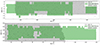 |
Fig. 1. Footprint of KiDS-1000 North (top) and South (bottom) as well as DES Y3 (overlap with KiDS South), HSC S19 (overlap with KiDS North), and the eRASS1 cluster sample. |
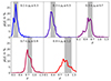 |
Fig. 2. Five spectroscopically calibrated tomographic redshift bins of KiDS. The redshift resolution is 0.05. We colour-coded the low-redshift tomographic bins blue and the high-redshift bins red, a convention that we preserve throughout this work. |
2.2. DES Y3
The Dark Energy Survey is a large optical survey covering 5000 deg2 on the sky, and it has significant overlap with the KiDS-South field. In this analysis, we make use of the data from the first three years of observations (hereafter DES Y3). DES is conducted using the Blanco telescope at the Cerro Tololo Inter-American Observatory (CTIO) in Chile. This 4 m telescope is equipped with a survey imaging instrument, DECam (Flaugher et al. 2015), that collects data in the grizY-bands.
The DES Y3 weak-lensing data products provide information for roughly 100 million galaxies (after selection cuts). They include a shape catalogue (Gatti et al. 2021) generated with the METACALIBRATION pipeline (Sheldon & Huff 2017) as well as photometric data (Sevilla-Noarbe et al. 2021). Further information about the point-spread function modelling can be found in Jarvis et al. (2021). (For details about image simulations see MacCrann et al. 2022).
Similarly to KiDS, DES makes use of a tomographic approach (Myles et al. 2021) that was originally developed for the DES 3 × 2 pt effort and is tightly integrated into the image simulations and calibration process. We refer to Grandis et al. (2024) for information about the shear measurement of eRASS1 galaxy clusters in DES Y3.
2.3. HSC-Y3
The HSC survey is a deep optical imaging survey that is carried out as part of the Subaru Strategic Program using the 8.2 m Subaru Telescope (Aihara et al. 2018). The Subaru Telescope is equipped with the HSC (Miyazaki et al. 2015, 2018), a specialised imager with a field of view of 2.3 deg2 surveying in the grizy-bands.
The aim of the HSC survey is to cover 1100 deg2 on the northern sky in its WIDE layer (there is also a DEEP and an UltraDEEP layer), and it has overlap with the KiDS-North field. The 5σ limiting magnitudes of the WIDE layer are 26.5, 26.1, 25.9, 25.1, and 24.4 in the g-, r-, i-, z-, and y-bands; thus, it represents the deepest imaging survey at this area to date. The HSC survey also provides great imaging quality, reaching a mean seeing of  in the i-band, which is used for shape measurement.
This analysis uses data products that stem from the three-year shape catalogue (HSC-Y3; Li et al. 2022), which has an effective galaxy number density of 19.9 arcmin−2. The shape measurement closely follows the methods employed in the analysis of the first-year HSC survey shape data (S16A, Mandelbaum et al. 2018a). We refer to Mandelbaum et al. (2018b) for further information about the shape calibration against simulations and to Oguri et al. (2018) for map level tests. Only galaxies with an i-band magnitude smaller than 24.5 mag are included in the shape catalogue. The HSC weak-lensing analysis around eRASS1 clusters follows the same methodology as the HSC weak-lensing analysis of clusters from the eROSITA Final Equatorial Depth Survey (eFEDS, Chiu et al. 2022).
2.4. eRASS1 galaxy cluster catalog
The cluster sample analysed in this paper stems from the first eROSITA All-Sky Survey in the western Galactic hemisphere (eRASS1), which was finished on June 11, 2020. We use the cosmology sample described in Bulbul et al. (2024), which consists of significantly extended X-ray sources with reliable photometric confirmation and redshift estimates in the range of 0.1 < zcl < 0.8, using the DESI Legacy Survey DR10 (Dey et al. 2019). As further detailed in Kluge et al. (2024), an adaptation of the redMaPPer (Rykoff et al. 2014, 2016; Rozo et al. 2015) algorithm, a red-sequence cluster finder designed for large photometric surveys, was employed to obtain redshift and richness estimates for eRASS1 cluster candidates.
In total, the cosmology sample contains 5263 clusters and groups, of which 237 have overlap with KiDS-1000 (101 in KiDS-North and 136 in KiDS-South). At this point, we already excluded objects that have a masked fraction larger than 50% in the shear measurement area in KiDS-1000 from our analysis. We show the cluster redshifts and the richnesses of the KiDS-1000 eRASS1 WL sample in Fig. 3 along with a division into three sub-samples for later testing purposes.
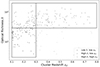 |
Fig. 3. Richness and redshift distribution of the eRASS1 clusters located in the KiDS-1000 footprint. Also included is a division into sub-samples for the tests presented in Sect. 3.2. |
3. Measurement
3.1. Shear measurement
We measured the weighted-reduced tangential shear of the source galaxies separately in tomographic redshift bins. We used all the tomographic bins (for a given cluster) whose lower photo-z boundaries (grey bands in Fig. 2) are located above the cluster redshift. In the weak-lensing regime, galaxy ellipticities ϵ transform under a reduced shear g as
 (1)
(1)
where
 (2)
(2)
is related to the shear γ and the convergence κ (Bartelmann & Schneider 2001).
Since we do not know the original ellipticities of the galaxies ϵorig, we had to average the observed ellipticities ϵobs over larger background samples, and we assumed that their intrinsic orientations are random and not aligned with the cluster (see Sifón et al. 2015). In this case, the average observed ellipticity,
 (3)
(3)
provides an unbiased estimate for the local reduced shear. As with the ellipticity, the shear and the reduced shear can be decomposed into a tangential component and a cross-component:
 (4)
(4)
where Φ is the azimuthal angle of the background galaxy with regard to the cluster centre.
We employed eight radial (geometric) bins with a bin width of 250 kpc for our shear measurement, starting at 500 kpc, which led to an outer measurement radius of 2.5 Mpc. This radial range allowed us to have a good balance between measuring the signal and being less susceptible to biases that arise from deviations of the cluster halos from perfectly centred Navarro-Frenk-White (NFW) profiles (Navarro et al. 1996), especially when due to mis-centring (e.g. Grandis et al. 2021; Sommer et al. 2022, 2024).
We adopted the multiplicative shear bias correction from van den Busch et al. (2022, we display the values in Appendix A.1) and averaged the tangential ellipticities in each tomographic bin b and geometric annulus to obtain estimates for the tangential reduced shear:
 (5)
(5)
where wi terms are the individual lensing weights of the galaxies that originate from their shape measurements, ϵt, i are their tangential ellipticities with respect to the cluster centre, and mb is the multiplicative shear bias coefficient, which is slightly different but statistically consistent for each tomographic redshift bin (see Table A.1). In Eq. (5), the sum runs over all galaxies i that fall into redshift bin b and a 250 kpc-wide annulus around a projected radius R. Furthermore the lensing weights in KiDS-1000 are calibrated such that
 (6)
(6)
We show an exemplary tangential reduced shear profile in Fig. 4. Furthermore, visual inspection of the stacked reduced cross shear profiles of the whole cluster sample shows that they are consistent with zero and show no radial trend.
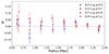 |
Fig. 4. Exemplary radial tangential reduced shear profile of the eRASS1 cluster em01_019120_020_ML00027_002_c947 in KIDS-1000 with a cluster redshift zcl = 0.16. We measured the shear separately in the tomographic background photo-z bins and plot the data points at the average projected radius of the contributing galaxies. |
3.2. Cluster member contamination
As we relied on photometric galaxy redshifts to select our background sources, cluster galaxies inevitably scattered into the selected galaxy sample that we used for our lensing measurement. These contaminating cluster galaxies suppress the shear that we measure since they are not lensed. Depending on the quality of the photo-zs (and other survey properties such as depth), the strength of the contamination varies and can become very significant, especially at small cluster-centric distances. This would lead to a mass that is biased low if we did not correct for this effect.
Past weak-lensing analyses have used different approaches to correct for cluster member contamination. For high-quality deep data, one can employ sufficient selection cuts in colour or photo-z space that effectively eliminate contamination (Schrabback et al. 2018a, 2021; Chiu et al. 2022). We did not follow this approach for KiDS for two reasons. First, it would require very stringent cuts, thus significantly shrinking the source sample. Second, a custom source selection would require tailored redshift and shear calibration efforts and would not allow us to employ the calibration results obtained for cosmic shear (Hildebrandt et al. 2021; van den Busch et al. 2022)3.
Gruen et al. (2014) pioneered the decomposition of field and cluster galaxy populations based on their multi-band colours. This approach led to the P(z) decomposition that is prominently employed in the weak-lensing analysis of DES (Varga et al. 2019; Grandis et al. 2024). This method is applicable when analysing larger cluster samples, but it is noisy for studies analysing smaller samples or clusters individually.
Alternatively, one can calculate the number density of the selected sources and use an observed increase towards the cluster centre as a measure of the contamination (e.g. Hoekstra 2007; Israel et al. 2010; Applegate et al. 2014; Schrabback et al. 2018b; Herbonnet et al. 2020). This is the approach that we follow in this work for the KiDS-1000 analysis.
3.2.1. Radial number density profiles
We measured the radial number density profiles of the source galaxies around eRASS1 clusters in KiDS-1000 ngx for each selected photometric redshift bin in 250 kpc-wide annuli (similar to the shear measurement), weighted with the individual galaxy lensing weights wi,
 (7)
(7)
where Aunmasked(R) is the unmasked geometric area of a given annulus. This incorporates the high-resolution pixel mask (6″ pixel side-length) of KiDS to account for masked areas in the shear catalogue. Furthermore, we approximated the corresponding Poisson errors as
![Mathematical equation: $$ \begin{aligned} \sigma \left[n_{\rm gx}(R)\right] =\frac{\sum _i { w}_i}{A_{\rm unmasked}(R)\sqrt{N_{\rm gx}(R)}}, \end{aligned} $$](/articles/aa/full_html/2025/03/aa49599-24/aa49599-24-eq12.gif) (8)
(8)
where Ngx is the number of galaxies in a given bin. We then normalised the background galaxy number density to the value that we find in the outer part of the cluster field, between 3.0 Mpc and 3.5 Mpc. We chose this radial range to measure the reference source number density, as going to larger radii can cause the cluster field of the lowest redshift clusters in the sample (zcl = 0.1) to cover even more than four KiDS-1000 tiles. Furthermore, visual inspection of the number density profiles showed that we can expect a negligible amount of contamination at these radii.
In case the cluster extends across multiple KiDS pointings (which can have significantly different number densities due to depth and seeing variations), we calculated the reference galaxy number density n0 on a per-annulus basis. We measured the fraction of the unmasked area that each pointing p contributes to a given annulus Aunmasked, p(R)/Aunmasked(R) and merged the respective reference number densities of the contributing pointings n0, p accordingly:
 (9)
(9)
We show one of the cluster fields and the corresponding radial field composition in Fig. 5 as well as the resulting radial number density profile in Fig. 6. The low-redshift tomographic bins show an especially pronounced increase in galaxy number density towards the cluster centre due to cluster member contamination, while the high-redshift tomographic bins show a decrease due to obscuration4.
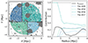 |
Fig. 5. Annuli around the cluster centres can have varying contributions from different tiles of the KiDS mosaic. Left: Exemplary cluster field the of eRASS1 cluster em01_019120_020_ML00027_002_c947, which covers four KiDS pointings. The grey areas are masked in KiDS-1000. Right: Fraction of unmasked area that each pointing contributes to a given annulus and fraction of masked pixels. |
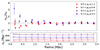 |
Fig. 6. Exemplary weighted & normalised radial number density profile for the eRASS1 cluster em01_046120_020_ML00096_002_c947 in KiDS-1000 with zcl = 0.25, λ = 50.9, uncorrected for obscuration. One can observe an increase in the normalised source density for the low-redshift tomographic bin towards the cluster centre due to cluster member contamination. The high-redshift tomographic bins show a decrease in source density due to obscuration from cluster galaxies. The bottoms panel shows the corresponding varying reference number density (weighted with lensing weights). |
3.2.2. Object detection bias
Clusters represent large optical over-densities on the sky. As a result, cluster galaxies obscure the sky and impede the detection of background galaxies. This also affects the galaxy number density profile and can even lead to an overall decrease towards the cluster centre. This can especially happen in the high-redshift tomographic bins (compare Fig. 6), which contain faint galaxies and are not subject to heavy contamination in the first place.
To account for this additional bias, we injected simulated KiDS-like galaxy images into the real r-band detection images of KiDS-1000 around each eRASS1 cluster. We used GalSim (Rowe et al. 2015) to generate the galaxy images as a convolution of a Sérsic profile for the galaxy itself and a Moffat profile to model the atmospheric seeing (Trujillo et al. 2001). We drew galaxies from the KiDS-1000 WL catalogue itself in order to attain the galaxy properties needed for the image simulation, such as half-light radius (HLR), r-band flux, and ellipticity. An exception is the Sérsic index, which is not contained in the KiDS-1000 WL catalogue. We drew the Sérsic index randomly from the 2DPHOT KiDS structural parameter catalogue (La Barbera et al. 2008; Roy et al. 2018; Amaro et al. 2021). However the KiDS-1000 catalogue is not complete at faint magnitudes. To simulate a complete population of galaxies based on the KiDS-1000 WL catalogue, we added a selection weight based on the galaxies’ r-band magnitude and HLR such that we drew faint and extended galaxies (which have a lower signal-to-noise ratios) more often. We obtained this selection weight by injecting ∼2 × 10+6 galaxies of different magnitudes and HLR’s into KiDS-1000 r-band images and analysing their detection probability with regard to these quantities.
We performed several image injection runs around each cluster, adding 15% additional galaxies in each tomographic bin in each run (relative to the overall number densities of the corresponding KiDS pointing in the different tomographic bins) until we injected at least 50 000 galaxies in each tomographic bin. We then re-ran the object detection software SExtractor (Bertin & Arnouts 1996) with the settings that the KiDS-consortium used to produce the KiDS-1000 WL catalogue. Since we knew at which positions we injected the galaxy images (as well as their original lensing weight in the WL catalogue), we could calculate the weighted radial detection probability profile d(R) for each cluster. We investigated the average lensing weight per galaxy in the KiDS-1000 WL catalogue around galaxy clusters as a function of cluster-centric distance and found no statistically significant change. We therefore argue that blending does not affect the lensing weights significantly in the context of this analysis.
To calculate the weighted radial detection probability profiles we averaged the ratio of re-detected to injected galaxies at a given annulus (and tomographic bin) over all injection runs, weighted with the lensing weights. Since the positions of the injected galaxies are random, the individual injection runs injected a varying number of galaxies in a given annulus. Thus, we weighted the detection ratios of the individual injection runs dk(R) at a given annulus (and tomographic bin b) with the number of injected galaxies Ninj, k(R) of that run (into this annulus and tomographic bin) when we averaged over all runs k:
 (10)
(10)
 (11)
(11)
where the wi terms are again the lensing weights. We calculated the corresponding run-to-run variance as an uncertainty:
 (12)
(12)
Furthermore, we normalised the weighted radial detection probability profiles analogously to the number density profiles, employing a reference detection probability d0(r) on a per-annulus basis, which we measured in the same outer radial, range 3.0 − 3.5 Mpc, for each KiDS-1000 pointing that contributes to the cluster field (see Fig. 7 for an example).
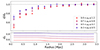 |
Fig. 7. Exemplary weighted radial detection probability profile of the eRASS1 cluster em01_022120_020_ML00040_002_c947. The bottom panel shows the corresponding varying reference detection probability (weighted with lensing weights). |
We fit all individual detection profiles simultaneously with a global model that we based on the cluster redshifts and optical richnesses λ according to
 (13)
(13)
where Rs is a characteristic scale radius and α, β, and R0 are parameters of the global fit. We found the following best-fit parameters: R0 = (0.709 ± 0.023) Mpc, α = 0.378 ± 0.050, and β = −0.174 ± 0.038. The negative exponent in the relation of the scale radius is a result of the degeneracy between α and β.
We calculated the amplitude of the object detection bias f(zcl) for every tomographic background galaxy bin based on a linear interpolation between pivot points in the cluster redshift space, which are also parameters of the global fit (Fig. 8). The pivot points have a redshift separation of 0.2, except for the last point in the highest redshift tomographic bin (Δz = 0.1), as the eRASS1 cosmology cluster sample does not extend to redshifts above 0.8.
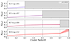 |
Fig. 8. Best-fit parameters of the redshift evolution of the object detection bias from the global fit of all individual radial detection profiles. |
To check if our global model fits the data, we split the eRASS1 cluster sample into three sub-samples in cluster redshift and optical richness bins (cf. Fig. 3). We averaged all the measurements (clusters of the sub-sample) at each radius and calculated the corresponding model values from the best-fit detection model based on the individual cluster redshifts and richnesses. We also averaged the calculated model values, and we show the result in Fig. 9. We excluded the innermost annulus 0 − 250 kpc (as well as the radial range of the baseline detection probability measurement 3.0 − 3.5 Mpc) from the fitting range, as the measured profiles drop steeply at the cluster centre. We argue that this is due to the brightest cluster galaxies (BCGs), which are usually located at the cluster centre and cause large object detection biases.
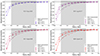 |
Fig. 9. Measured and best-fit radial detection profiles stacked separately for the different tomographic source bins (panels) and divided into three cluster sub-samples. |
We observed that the strength of the object detection bias increases with cluster redshift and richness in all tomographic bins. It also increases slightly for high-redshift tomographic bins compared to low-redshift ones. At a cluster-centric distance of 1 Mpc, the weighted radial detection probability profiles typically show an effective object detection bias of 4−10%. At 500 kpc, this increases to up to 15% for the high-redshift, high-richness cluster sub-sample. Furthermore we can confirm that the global model describes the measured detection profiles well.
3.2.3. Contamination model
We subsequently used the best-fit detection probability model to boost the measured radial number density profiles based on the individual cluster redshifts and richnesses
![Mathematical equation: $$ \begin{aligned} \left(\frac{n(R)}{n_0(R)}\right)^\mathrm{corr}=\frac{n(R)}{n_0(R)}\left[1+f(z_{\rm cl})\left(\frac{\lambda }{25}\right)^{\alpha }e^{1-R/R_{\rm s}}\right]. \end{aligned} $$](/articles/aa/full_html/2025/03/aa49599-24/aa49599-24-eq18.gif) (14)
(14)
We applied Gaussian error propagation and in turn performed a second global fit on these boosted number density profiles to extract the final contamination model
 (15)
(15)
We found R0′ = 0.927 ± 0.079 Mpc, α′ = 0.644 ± 0.086, and β′= − 0.303 ± 0.096. The uncertainties are larger than for the detection model because we only have one realisation for each cluster, compared to several hundred image injection runs.
Figure 10 shows the amplitude parameter of the contamination model f′(zcl) at pivot points in the cluster redshift space. Here, the uncertainties are estimated by bootstrapping over the cluster sample to additionally account for the correlations in the galaxy counts between different radial bins that are caused by LSS fluctuations. We observed that the highest redshift tomographic bin (0.9 < zB ≤ 1.2) is effectively contamination-free within our measurement uncertainty. We expect this behaviour, as the contamination should increase for clusters that approach the lower border of the tomographic bin in redshift space. There are no clusters with a redshift above 0.8 in the eRASS1 cluster sample, and the highest redshift tomographic bin only starts at a photo-z of 0.9.
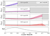 |
Fig. 10. Best-fit result of the amplitude parameter of the global contamination model at pivot points in the cluster redshift space. Bottom: Distribution of the eRASS1 KiDS-1000 cluster redshifts. |
The tomographic bin 0.7 < zB ≤ 0.9 shows significant contamination for zcl > 0.5, which we expect due to analogous reasoning. However, the majority of eRASS1 clusters are located at lower cluster redshifts.
The tomographic bin 0.5 < zB ≤ 0.7 starts to show more contamination at lower cluster redshifts. We trace this back to the individual redshift distributions of the tomographic bins (Fig. 2). This particular tomographic bin shows a pronounced wing towards lower redshifts; that is, a large portion of galaxies in this photo-z range populate lower actual redshifts, which leads to a stronger contamination.
The low-redshift tomographic bin (0.3 < zB ≤ 0.5) only shows contamination for zcl > 0.2, and negative contamination for cluster redshifts that are lower. This is an indication that our image injection analysis did not capture the full effect that cluster galaxies have on background galaxies in this tomographic bin, at least for very low cluster redshifts. As a general rule, we observed that cluster member contamination starts to become pronounced if the redshift separation between the cluster and tomographic bin is Δz ≲ 0.2.
We proceeded in a similar manner to the stacking method that we described previously for the global fit of the detection profiles in order to check our global fit of the boosted number density profiles. We re-used the three cluster sub-samples divided by cluster redshift and richness but employed inverse-variance weighting for the individually normalised corrected number densities in each annulus. We propagated these inverse-variance weights when we calculated the average of the corresponding model values. We chose a weighted average this time because the unweighted average would be biased high due to some values that up-scatter significantly (but have large absolute uncertainties and therefore a low impact on the global fit).
We note that this method of stacking (using the inverse-variance weights) emphasises number density profiles that scatter low. This is due to the Poisson errors, as data points with a few galaxies will have a low absolute uncertainty and subsequently a high weight contribution to the average. This weighted average does, however, allow us to verify if the global fit describes the data. We show the result in Fig. 11.
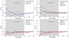 |
Fig. 11. Measured and best-fit detection-corrected radial number density profiles stacked in tomographic bins (different panels) and divided into three cluster sub-samples. We employed inverse-variance weighting to take the average at each radius, which pronounces clusters as scattering low. |
As we discussed previously, it becomes evident that the image injection analysis, which we used to account for the object detection bias, does not fully capture the effect in the lowest tomographic bin (0.3 < zB ≤ 0.5). We observed a dip in the stacked profiles below the baseline before the contamination dominates at small cluster-centric distances. While some of this can be attributed to the inverse-variance weights of the stacked number density profiles, we did not observe such a behaviour to this extent in the other tomographic bins.
This dip below the baseline in the stacked profiles, together with the redshift evolution of the amplitude parameter of the contamination model in this tomographic bin (Fig. 10), is enough reason for us to not use the shear measurement in this tomographic bin in our further analysis and mass calibration. This tomographic bin has a low effective lensing efficiency. Hence, we did not lose a lot of lensing signal by disregarding it. Moreover, we wanted to ensure that the cluster member contamination correction is as accurate as possible when we perform consistency checks with DES and HSC and want to provide accurate shear measurements for the eRASS1 WL mass calibration.
As expected from its redshift distribution (Fig. 2), the tomographic bin 0.5 < zB ≤ 0.7 shows the most contamination. The stacked number density profiles in the two high-redshift tomographic bins are nearly contamination-free (the tomographic bin 0.7 < zB ≤ 0.9 shows some contamination in the high-redshift, high-richness clusters sub-sample at small radii).
We show the best-fit contamination model at a cluster-centric distance of 1 Mpc for two cluster richnesses (λ = 80 and λ = 15) as a function of the cluster redshift in Fig. 12.
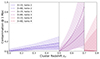 |
Fig. 12. Best-fit contamination model for richness 15 and 80 at a cluster-centric distance of 1 Mpc as a function of the cluster redshift and always showing the lowest included tomographic source bin only. Here, we set amplitude parameters f′(zcl) that scatter to negative values to zero, which mirrors the treatment of the contamination model in Appendix A.1. |
To account for the contamination in the further analysis, one can either rescale the individual shear profiles or include the contamination in the computation of the weak-lensing mass bias bWL. We followed the latter approach for our main analysis, which allowed us to easily propagate the uncertainty in the fit of the global contamination model (see Appendix A.1).
4. Consistency checks with DES Y3 and HSC S19
In this section, we compare the WL results obtained on eRASS1-selected clusters using the KiDS-1000 survey, DES (Grandis et al. 2024), and the HSC survey (Ghirardini et al. 2024, Sect. 2.3.1). We perform this comparison both at the level of individual density contrast estimates and amplitudes as well as at the level of the global scaling relation fit.
4.1. Contamination-corrected shear profiles
Within the western Galactic hemisphere, the KiDS-1000 survey has a footprint overlap with DES and the HSC survey (Fig. 1). The direct overlap between HSC and DES falls in the eastern Galactic hemisphere, and thus it is outside of the region where the eROSITA-DE consortium is analysing the X-ray data. The overlap of the surveys provides a unique opportunity to validate cluster WL measurements from different lensing surveys around the lensed clusters selected in a coherent manner.
Given the different source redshift distributions and the different degrees of cluster member contamination, this comparison is best conducted on the estimates for the density contrast profiles ΔΣ(R) = Σcrit, eff ⟨γt⟩(R). Here, ⟨γt⟩(R) is estimated from the contamination-corrected azimuthally averaged tangential shear estimates5, while differences in the source redshift distributions are accounted for via the effective critical surface mass density Σcrit, eff, which is computed by adequately averaging (see below) the source and lens redshift-dependent inverse critical surface mass density:
 (16)
(16)
Equation (16) includes the Heaviside step function H(x), the gravitational constant G, the speed of light in vacuum c, and the angular diameter distances between the observer and the lens Dl, the observer and the source Ds, and the lens and the source Dls.
Comparing the density contrast estimates of the same lenses measured in two WL surveys poses the challenge that the surveys will have some selected source galaxies in common. The shape noise contributions from these sources will be partially correlated, as the intrinsic shape of a common source is the same6, while the shape measurement error will be different. Working only on sources selected by both surveys is, in principle, possible (Hoekstra et al. 2015), but it would require re-calibrating the shape measurement and photo-z uncertainties for the new joint selection, as the source redshift and shape calibrations are only valid for specific survey-internal source selections. These selection criteria would be broken when working on a jointly selected background galaxy sample.
To solve this problem, we constructed the ‘union’ of the source catalogues from KiDS and DES around each eRASS1 cluster (and KiDS and the HSC survey, respectively). The sources from the two surveys that fall within 1 arcsec of each other were considered selected by both surveys and successively treated as one source with two sets of measurements. Naturally, other sources were selected by only one of the surveys. We thus constructed two union samples: DES-KiDS around 125 eRASS1 clusters and HSC-KiDS around 48 eRASS1 clusters. Compared to previous cluster WL comparisons, our approach has the benefit of being able to rely on the high accuracy of the shape and photo-z calibration of the respective wide-area WL surveys.
We estimated the density contrast from the DES sources as
 (17)
(17)
where fcl(R|zl, λ) is the best-fit cluster member contamination profile derived in Grandis et al. (2024, Sect. 3.3.1), which is a function of a cluster-centric distance R, cluster richness λ, and cluster redshift zl. The sum over i runs over all selected DES sources i in the respective radial bin, and wbi is the weighting of the sources’ tomographic redshift bin bi, which implements the DES background selection (Grandis et al. 2024, Sect. 3.2). The critical density of the tomographic bin was computed as  , where P(zs|b) are the source redshift distributions calibrated by Myles et al. (2021). We note that they are normalised to the multiplicative shear bias correction of that tomographic bin. Our implementation thus corrects for the multiplicative shear bias.
To estimate the surface mass density from the HSC source data, we used the source sample whose selection follows Chiu et al. (2022), as reported in Ghirardini et al. (2024, Sect. 2.3.1). Specifically,
 (18)
(18)
where 𝒦 = ∑iwismi/∑iwis is the source-weighted average multiplicative shear bias and ℛ = 1 − ∑iwiserms, i2/∑iwis. In light of the stringent background selection implemented, the HSC WL measurements have a cluster member contamination that is consistent with zero. For the HSC analysis, we computed individual estimates for the critical surface mass density Σcrit, li for each source i from a Monte Carlo realisation of DEmP photo-z estimates (Hsieh & Yee 2014), which yielded unbiased estimates of Σcrit at the ≲1% level out to cluster redshifts zcl ∼ 0.6 (Chiu et al. 2022).
For the KiDS data, we estimated the density contrast for each tomographic bin b as
 (19)
(19)
with  being the cluster member contamination model of each tomographic bin,
  constituting the average inverse critical surface mass density of that tomographic bin, and mb being the mean multiplicative shear bias of the respective bin, listed in Table A.1.
On an individual cluster basis, our test statistic is the difference between the DES and KiDS density contrasts,
 (20)
(20)
for each KiDS tomographic bin b and the difference between the HSC and KiDS density contrasts,
 (21)
(21)
The statistical errors δΞ(R) of these profiles need to be extracted by bootstrapping on the unions of the respective source samples. Specifically, this means that if in a bootstrap we draw a source present in both surveys, it needs to be coherently included in both parts of the difference. We also note that by bootstrapping on the union of the samples, we are still bootstrapping on a fair sample of either survey’s selection. This means that selection-dependent calibration products are still valid. Furthermore, this technique allows us to account for the correlated shape noise correctly.
In Fig. 13 we show the sample-averaged difference as a function of cluster-centric distance in the reference cosmology in the left panels, and the inverse-variance-scaled squared deviation of our test statistics from zero
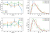 |
Fig. 13. Consistency test between the density contrast profiles of clusters observed both in DES (HSC) and KiDS in the upper (lower) panels. Given the correlated intrinsic galaxy shapes, we constructed the statistical uncertainty estimates by bootstrapping on the union of the respective source catalogues. We find that, averaged over all objects, the estimates from the survey pairs are consistent as a function of radius (left column). Also, the uncertainty weighted mean square deviation of all clusters, shown in the right column, is consistent with the expectation (red curve). |
 (22)
(22)
is shown in the right panels. The latter is compared with the expected distributions if Ξ(R)∼𝒩(0, δΞ(R)2), which is from a random normal with mean zero and the variance given by the square of the bootstrap error we determined. This is a chi-squared distribution with six degrees of freedom, as we chose six radial bins. Compressing the left panels of Fig. 13 further into a single global number by averaging over KiDS tomographic bins and cluster-centric distances, we found relative differences of −0.151 ± 0.067 (2.3σ) and 0.312 ± 0.078 (4σ) between DES versus KiDS and HSC versus KiDS, respectively. The difference between KiDS and HSC is significant and warrants future tests. The significances in the individual tomographic bins of KiDS are smaller due to the increased noise.
4.2. Scaled Einstein radius comparison
To test for redshift and richness trends in the WL signal of clusters observed by the two surveys, we expanded on the Einstein radius comparison proposed in Hoekstra et al. (2015). That comparison was based on the fact that for a mass distribution following an isothermal sphere, the tangential shear profile takes the form  , where RE is the mean Einstein radius of the source sample. Ignoring the reduced shear correction, the mean Einstein radius can be directly obtained using an estimator of the form ⟨2ϵtR⟩, thus providing a convenient measure of the overall strength of the WL signal around a lens and avoiding having to split the lensing signal into radial bins, as done in Sect. 4.1.
In order to account for the different source redshift distributions of our source samples, we altered the original prescription by Hoekstra et al. (2015) to estimate the amplitude AISO of an isothermal density profile in physical units, which we define as
 (23)
(23)
where θ is the cluster-centric distance in angular units. Direct comparison to the expression from Hoekstra et al. (2015) revealed that AISO is just a critical surface density-corrected Einstein radius in angular units, which can therefore be readily compared between source samples with different geometrical lensing configurations.
To estimate this quantity in the three different surveys we consider, we set up the following inverse-variance weigthed estimators. For DES, we computed
 (24)
(24)
where  is the cluster member contamination evaluated for the ith source. We note that this estimator scales the tangential reduced shear of each source i with Σcrit, lbiθi/
 , which is in line with the naive inversion of Eq. (23) in the presence of cluster member contamination.
For HSC, where Chiu et al. (2022) found no cluster member contamination and where we have reliable individual photometric redshift estimates, we computed
 (25)
(25)
Similarly, for each KiDS tomographic redshift bin b, we could compute
 (26)
(26)
with the cluster member contamination estimate  for each individual source.
As a test statistic, we then considered the difference between the amplitude estimates in HSC and KiDS as well as in DES and KiDS for the clusters that have data in two of the respective surveys. The statistical uncertainty on these differences was estimated by bootstrapping on the union of the source samples, as discussed in Sect. 4.1.
In Fig. 14, we present in the left (right) panel the distribution of the difference in isothermal sphere amplitudes between DES and KiDS (HSC and KiDS) for the different KiDS tomographic redshift bins, plotted relative to the uncertainty of this difference as a function of cluster redshift and richness. In black, the figure also shows averages computed over equally spaced bins including the respective error bars. We found excellent agreement between these estimates, with the overall mean also reported in Table 1. Furthermore, visual inspection revealed no redshift and richness trends.
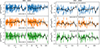 |
Fig. 14. Difference in the amplitude of the isothermal sphere shear profile models fitted to clusters with coverage by DES and KiDS (HSC and KiDS) in the left (right) panel plotted relative to the uncertainty of this difference and as a function of cluster redshift and richness (columns) for the different KiDS tomographic redshift bins (rows). We found excellent overall agreement, while no richness or redshift trends are evident from visual inspection, also after binning (black points). |
Sample averaged differences in the amplitudes of scaled isothermal sphere shear profiles relative to the uncertainty of the differences measured in DES and HSC with regard to KiDS estimates based on different tomographic redshift bins.
Compared to the test in the previous section, this test places more focus on the outer parts of the profile due to the θ weighting in the estimator. This regime is less impacted by cluster member contamination and obscuration of background sources and focuses on the scales where the bulk of the signal originates. It is therefore very encouraging to find such good agreement among the estimates from the different surveys.
4.3. Scaling relations
Using the Bayesian population model described in Grandis et al. (2024, Sect. 5.1) and Ghirardini et al. (2024, Sect. 4), we derived constraints on the parameters of the scaling between the eROSITA count rate and the halo mass and redshift, which is defined as follows:
 (27)
(27)
where CR, b = 0.1 is the pivot value for the count rate, Mb = 2 × 10¹⁴ M⊙ is the pivot value for the mass, and zb = 0.35 is the pivot value for the redshift. The term bX(M, z) expresses the mass-redshift dependent slope of the scaling relation, which is given by
where BX is the classic standard single value mass slope, CX allows the slope to be mass dependent – but is kept fixed to zero in this analysis, and FX allows the slope to be redshift dependent. The redshift evolution term, ex(z), is given by
 (28)
(28)
for which EX = 2 and DX = −2 are the values adopted by the self-similar model (Kaiser 1986) for the case of luminosity.
As described in more detail in Grandis et al. (2024), Sect. 5.1, and in Ghirardini et al. (2024), Sect. 4, we constructed a likelihood for the measured tangential reduced shear profile. Deviating from the other works, for the KiDS data, we considered one reduced shear profile  for each tomographic redshift bin b. The likelihood depends not only on the parameters of the count rate to halo mass relation but also on the cosmological parameters. We thus varied the present day matter density with regard to the critical density, ΩM = 0.331 ± 0.038, as determined by DES’s year 1 supernovae type Ia analysis (Abbott et al. 2019). We also varied the fraction of random sources and point sources in our likelihood with priors from the optical follow-up of eRASS1 clusters (Kluge et al. 2024; Ghirardini et al. 2024).
Another input is the calibration of the WL mass bias and scatter, which follows the prescriptions outlined in Grandis et al. (2024, Sect. 4). The adaptations to the KiDS-1000 WL specifications and the resulting numerical values for the WL bias and scatter are discussed in Appendix A.1.
By sampling the likelihood, we found the amplitude of the count rate to halo mass relation AX = 1.77 ± 0.42, the mass trend of the relation BX = 1.69 ± 0.27, its redshift trend FX = 1.57 ± 1.74, the deviation from a self-similar redshift evolution GX = −2.60 ± 1.47, and an upper limit on the intrinsic scatter of σX < 0.85 at the 97.5 percentile. The one- and two-dimensional marginal contours of the posterior are shown in green in Fig. 15 and are listed in Table 2.
Calibration of the count rate to halo mass relation parameters for eROSITA using different weak-lensing data sets and cluster samples.
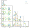 |
Fig. 15. One- and two-dimensional marginal contour plots for the WL mass calibration of the eROSITA count rate to halo mass relation. In green the results from KiDS-1000 on eRASS1 are shown, in blue are the results from DES Y3 on eRASS1 (Grandis et al. 2024), in orange are the results from HSC-Y3 on eRASS1, and in black are the results from HSC-Y3 on eFEDS (Chiu et al. 2022). All results show agreement, indicating the reliability of the WL mass calibration methods employed by the different teams. |
We repeated the same analysis also with the HSC-derived WL data set, which was extracted with the method described in Chiu et al. (2022) and outlined in Ghirardini et al. (2024, Sect. 2.3.1). The WL bias and scatter for HSC are reported in Appendix A.2. With that data set, we found the amplitude of the observable–mass relation AX = 0.77 ± 0.32, the mass slope BX = 1.65 ± 0.35, its redshift trend FX = 1.20 ± 1.66, a deviation from self-similar redshift evolution of GX = −1.24 ± 1.60, and an intrinsic scatter of σX = 0.72 ± 0.25. These results are shown as orange contours in Fig. 15 and reported in Table 2.
Given that all three mass calibration analyses have a coherent WL bias correction and calibrate the same astrophysical relation between the eROSITA count rate and halo mass, we could directly compare the results on the scaling relation parameters from KiDS and HSC with the DES results (see Fig. 15 in blue and Grandis et al. 2024, see Fig. 15 in blue and). We found that the mass calibrations from all three surveys are statistically consistent with each other and with the results found by Chiu et al. (2022) with HSC on eFEDS clusters. We quantified this agreement by following the prescription of Raveri & Doux (2021) based on the posterior of parameter differences and the probability mass of a difference consistent with zero. We found that in our case, the Gaussian limit holds for the posterior of parameter differences. Turning this probability mass into a tension in sigmas, we found 0.91σ of tension between the scaling relation parameter posteriors from HSC and KiDS (without eFEDS), 2.12σ between KiDS and DES, and 0.23σ between DES and HSC. The analyses in the three surveys have been performed on different data sets with different modelling choices. Their agreement validates the choices in the modelling, and it demonstrates the reliability of the WL mass calibration of clusters in the context of stage-III surveys.
4.4. Goodness of fit
To inspect the goodness of fit, we followed the same procedure as in Grandis et al. (2024, Sect. 5.2). We refer the reader to that section for the exact definitions of the stacking procedure. Differing from that work, for the KiDS data, we defined the stacking weight for the cluster 𝜘 as  for each tomographic bin b in KiDS. We also only considered three redshift bins (0.1, 0.3, 0.5, 0.8) and no binning in count rate. The rest of the procedure is the same. Figure 16 shows that the jointly constrained model describes the measured tangential reduced shear profiles well for all KiDS tomographic redshift bins, with a chi-squared of
  with 63 data points, three well-constrained model parameters, and two upper limits. The figure therefore also provides a confirmation that the cluster weak-lensing signal indeed scales with the source redshift, as expected within the employed reference ΛCDM cosmology.
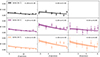 |
Fig. 16. Stacked tangential reduced shear profiles from KiDS-1000 for different tomographic redshift bins (rows) and cluster redshift bins (columns) together with the mean stacked model and its one sigma uncertainty (filled area). The mean stacked model incorporates the model for cluster member contamination, making the model prediction and the data directly comparable. The model fits the data very well. |
The HSC data were binned by using weights W𝜘 = 1/(δgt, 𝜘)2, where δgt, 𝜘 is the estimate for the uncertainty on the tangential reduced shear profile of the 𝜘th cluster. The clusters were then binned in redshift bins (0.10, 0.19, 0.27, 0.35, 0.48, 0.8) and count rate bins (0.01, 0.61, 16.1), for which we found a chi-squared of  with 70 data points and five well-constrained model parameters. The comparison of the HSC data and the best-fit model is shown in Fig. 17. Some stacked reduced shear profiles clearly deviate from the best-fit model, explaining the high χ2. Also, the best-fit model from the full cosmological analysis in Ghirardini et al. (2024) shows a bad fit for the HSC data. This is in line with the significant difference we find between the KiDS and HSC stacked profiles, reported in Sect. 4.1. The fit nonetheless qualitatively captures the trends in the data.
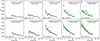 |
Fig. 17. Stacked tangential reduced shear profiles measured using the HSC data and split according to cluster count rate (rows) and cluster redshift bins (columns) together with the mean stacked model and its one sigma uncertainty (filled area). Not all the stacked reduced shear profiles result in statistically good fits (especially at low count rates), leading to a rather high χ2. |
5. Summary, discussion, and conclusion
We have presented our shear measurements around 237 clusters from the cosmology sample of the first eROSITA All-Sky Survey (eRASS1) in KiDS-1000. We measured the tangential reduced shear in eight geometric annuli (250 kpc-wide, 0.5 − 2.5 Mpc) separately for each tomographic redshift bin of KiDS. These tomographic bins have been defined for the KiDS cosmic shear analysis, which allows us to directly employ the shear and redshift calibrations derived by the KiDS teams for the KiDS cosmic shear analysis (Hildebrandt et al. 2021; van den Busch et al. 2022).
Furthermore, we measured and accounted for cluster member contamination via radial number density profiles of the background galaxies. This analysis included the injection of simulated galaxy images (using GalSim) into the r-band mosaics of KiDS-1000 in order to account for the obscuration caused by foreground and cluster galaxies. We presented a global model for both the radial detection probability and the corrected number density of background-selected sources (which is a measure of the contamination) for eRASS1 clusters in KiDS-1000 based on the cluster redshift and optical richness λ.
We find that the weighted detection probability typically decreases by 4−10% at a cluster-centric distance of 1 Mpc due to the obscuration, depending on the tomographic bin as well as the cluster redshift and richness. This would directly translate into identical biases in the number density profiles and boost-corrected reduced shear profiles if unaccounted for. We find that the cluster member contamination has a major impact if the cluster redshift and lower photo-z border of a tomographic bin have a separation of Δz ≲ 0.2.
The KiDS-1000 weak-lensing measurements described in this paper contribute to the joint constraints on cosmological parameters and the eROSITA count rate to halo mass scaling relation presented in Ghirardini et al. (2024), together with weak-lensing constraints from DES Y3 and HSC-Y3. In our paper, we have presented consistency checks for the weak-lensing based constraints obtained from the different data sets. In particular, we studied the differences in the differential surface mass density profiles obtained with different lensing surveys for common galaxy clusters. We find that the stacked WL signal from HSC is significantly higher than the KiDS one, while finding no significant difference between KiDS and DES. It would be interesting to contrast these findings with the biases in the photometric redshifts recently found by Rau et al. (2023), Chiu et al. (2024) for high-redshift HSC sources. To properly account for the highly correlated intrinsic galaxy shapes for common weak-lensing sources between different lensing surveys, we introduced bootstrapping conducted on the union of sources. We also compared the scaled Einstein radii estimates on an individual cluster basis, finding no indication for redshift- or richness-dependent biases among the surveys. Furthermore, we computed constraints on the eROSITA count rate to halo mass relation separately for the three weak-lensing surveys. Here, we find broadly consistent results, justifying the joint analysis presented in Ghirardini et al. (2024). Our analysis contributes to cross-survey comparisons between current stage-III weak-lensing surveys, such as the galaxy-galaxy lensing analysis presented in Leauthaud et al. (2022).
Finally, we presented stacked tangential reduced shear profiles for eRASS1 clusters both for the KiDS and HSC weak-lensing data. Our KiDS analysis conducted in different tomographic redshift bins demonstrates that the cluster weak-lensing signal scales with the source redshift, as expected in a standard ΛCDM cosmology, providing a further consistency check for the KiDS weak-lensing measurements.
Our analysis provides a demonstration for the mass calibration of large galaxy cluster samples using wide-area weak-lensing surveys. Here our strategy of using the same tomographic source bins employed for cosmic shear analyses provides a major advantage in that the shear and redshift calibration can be directly tied to the cosmic shear efforts. This, however, requires careful correction of the cluster member contamination. For this, we suggest that future analyses combine a detection-probability corrected number-density profile estimation as employed in our work with the photometric redshift decomposition introduced by Gruen et al. (2014) and as employed, for example, in the eRASS1 DES analysis by Grandis et al. (2024). Combining the two approaches provides an internal consistency check for this important source of systematic uncertainty.
The stronger shears and the higher level of blending present in cluster fields may have some impact on shear calibrations. However, the analysis by Hernández-Martín et al. (2020) suggests that this is at a level that can be safely ignored for our present analysis given the statistical uncertainty.
We estimate the impact of magnification on the source number densities in Appendix B, and we find it to be around the percent-level, which is subdominant to the impact of obscuration by cluster galaxies.
We approximated the shear with the reduced shear and ignored corrections from the convergence (see Eq. (2)) given the lack of a precise convergence profile estimate for each cluster. However, reduced shear corrections are correctly accounted for in the more constraining scaling relation comparison (see Sect. 4.3 and Grandis et al. 2024).
Slight differences may occur due to different resolutions in different data sets and different brightness profile weighting schemes employed by different shape measurement techniques.
References
- Abbott, T. M. C., Allam, S., Andersen, P., et al. 2019, ApJ, 872, L30 [Google Scholar]
- Abell, G. O. 1958, ApJS, 3, 211 [NASA ADS] [CrossRef] [Google Scholar]
- Aihara, H., Arimoto, N., Armstrong, R., et al. 2018, PASJ, 70, S4 [NASA ADS] [Google Scholar]
- Albrecht, A., Bernstein, G., Cahn, R., et al. 2006, ArXiv e-prints [arXiv:astro-ph/0609591] [Google Scholar]
- Allen, S. W., Evrard, A. E., & Mantz, A. B. 2011, ARA&A, 49, 409 [Google Scholar]
- Amaro, V., Cavuoti, S., Brescia, M., et al. 2021, in Intelligent Astrophysics, eds. I. Zelinka, M. Brescia, & D. Baron, 39, 245 [NASA ADS] [CrossRef] [Google Scholar]
- Angulo, R. E., Springel, V., White, S. D. M., et al. 2012, MNRAS, 426, 2046 [NASA ADS] [CrossRef] [Google Scholar]
- Applegate, D. E., von der Linden, A., Kelly, P. L., et al. 2014, MNRAS, 439, 48 [Google Scholar]
- Arnaboldi, M., Capaccioli, M., Mancini, D., et al. 1998, The Messenger, 93, 30 [NASA ADS] [Google Scholar]
- Astropy Collaboration (Price-Whelan, A. M., et al.) 2022, ApJ, 935, 167 [NASA ADS] [CrossRef] [Google Scholar]
- Bartelmann, M., & Schneider, P. 2001, Phys. Rep., 340, 291 [Google Scholar]
- Bertin, E., & Arnouts, S. 1996, A&AS, 117, 393 [NASA ADS] [CrossRef] [EDP Sciences] [Google Scholar]
- Bocquet, S., Dietrich, J. P., Schrabback, T., et al. 2019, ApJ, 878, 55 [Google Scholar]
- Bocquet, S., Heitmann, K., Habib, S., et al. 2020, ApJ, 901, 5 [Google Scholar]
- Bocquet, S., Grandis, S., Bleem, L. E., et al. 2024a, Phys. Rev. D, 110, 083509 [NASA ADS] [CrossRef] [Google Scholar]
- Bocquet, S., Grandis, S., Bleem, L. E., et al. 2024b, Phys. Rev. D, 110, 083510 [NASA ADS] [CrossRef] [Google Scholar]
- Bulbul, E., Chiu, I. N., Mohr, J. J., et al. 2019, ApJ, 871, 50 [Google Scholar]
- Bulbul, E., Liu, A., Kluge, M., et al. 2024, A&A, 685, A106 [NASA ADS] [CrossRef] [EDP Sciences] [Google Scholar]
- Chiu, I. N., Ghirardini, V., Liu, A., et al. 2022, A&A, 661, A11 [NASA ADS] [CrossRef] [EDP Sciences] [Google Scholar]
- Chiu, I.-N., Chen, K.-F., Oguri, M., et al. 2024, Open J. Astrophys., 7 [Google Scholar]
- de Jong, J. T. A., Kuijken, K., Applegate, D., et al. 2013, The Messenger, 154, 44 [NASA ADS] [Google Scholar]
- Dey, A., Schlegel, D. J., Lang, D., et al. 2019, AJ, 157, 168 [Google Scholar]
- Dietrich, J. P., Bocquet, S., Schrabback, T., et al. 2019, MNRAS, 483, 2871 [Google Scholar]
- Fenech Conti, I., Herbonnet, R., Hoekstra, H., et al. 2017, MNRAS, 467, 1627 [NASA ADS] [Google Scholar]
- Flaugher, B., Diehl, H. T., Honscheid, K., et al. 2015, AJ, 150, 150 [Google Scholar]
- Gatti, M., Sheldon, E., Amon, A., et al. 2021, MNRAS, 504, 4312 [NASA ADS] [CrossRef] [Google Scholar]
- Ghirardini, V., Bulbul, E., Artis, E., et al. 2024, A&A, 689, A298 [NASA ADS] [CrossRef] [EDP Sciences] [Google Scholar]
- Giblin, B., Heymans, C., Asgari, M., et al. 2021, A&A, 645, A105 [NASA ADS] [CrossRef] [EDP Sciences] [Google Scholar]
- Grandis, S., Bocquet, S., Mohr, J. J., Klein, M., & Dolag, K. 2021, MNRAS, 507, 5671 [NASA ADS] [CrossRef] [Google Scholar]
- Grandis, S., Ghirardini, V., Bocquet, S., et al. 2024, A&A, 687, A178 [NASA ADS] [CrossRef] [EDP Sciences] [Google Scholar]
- Gruen, D., Seitz, S., Brimioulle, F., et al. 2014, MNRAS, 442, 1507 [CrossRef] [Google Scholar]
- Harris, C. R., Millman, K. J., van der Walt, S. J., et al. 2020, Nature, 585, 357 [NASA ADS] [CrossRef] [Google Scholar]
- Herbonnet, R., Sifón, C., Hoekstra, H., et al. 2020, MNRAS, 497, 4684 [NASA ADS] [CrossRef] [Google Scholar]
- Hernández-Martín, B., Schrabback, T., Hoekstra, H., et al. 2020, A&A, 640, A117 [EDP Sciences] [Google Scholar]
- Hildebrandt, H., Köhlinger, F., van den Busch, J. L., et al. 2020, A&A, 633, A69 [NASA ADS] [CrossRef] [EDP Sciences] [Google Scholar]
- Hildebrandt, H., van den Busch, J. L., Wright, A. H., et al. 2021, A&A, 647, A124 [EDP Sciences] [Google Scholar]
- Hoekstra, H. 2007, MNRAS, 379, 317 [NASA ADS] [CrossRef] [Google Scholar]
- Hoekstra, H. 2013, ArXiv e-prints [arXiv:1312.5981] [Google Scholar]
- Hoekstra, H., Herbonnet, R., Muzzin, A., et al. 2015, MNRAS, 449, 685 [NASA ADS] [CrossRef] [Google Scholar]
- Hsieh, B. C., & Yee, H. K. C. 2014, ApJ, 792, 102 [Google Scholar]
- Hunter, J. D. 2007, Comput. Sci. Eng., 9, 90 [NASA ADS] [CrossRef] [Google Scholar]
- Israel, H., Erben, T., Reiprich, T. H., et al. 2010, A&A, 520, A58 [NASA ADS] [CrossRef] [EDP Sciences] [Google Scholar]
- Jarvis, M., Bernstein, G. M., Amon, A., et al. 2021, MNRAS, 501, 1282 [Google Scholar]
- Kaiser, N. 1986, MNRAS, 222, 323 [Google Scholar]
- Kannawadi, A., Hoekstra, H., Miller, L., et al. 2019, A&A, 624, A92 [NASA ADS] [CrossRef] [EDP Sciences] [Google Scholar]
- Kluge, M., Comparat, J., Liu, A., et al. 2024, A&A, 688, A210 [NASA ADS] [CrossRef] [EDP Sciences] [Google Scholar]
- Kuijken, K. 2011, The Messenger, 146, 8 [NASA ADS] [Google Scholar]
- Kuijken, K., Heymans, C., Dvornik, A., et al. 2019, A&A, 625, A2 [NASA ADS] [CrossRef] [EDP Sciences] [Google Scholar]
- La Barbera, F., de Carvalho, R. R., Kohl-Moreira, J. L., et al. 2008, PASP, 120, 681 [NASA ADS] [CrossRef] [Google Scholar]
- Le Brun, A. M. C., McCarthy, I. G., Schaye, J., & Ponman, T. J. 2014, MNRAS, 441, 1270 [NASA ADS] [CrossRef] [Google Scholar]
- Leauthaud, A., Amon, A., Singh, S., et al. 2022, MNRAS, 510, 6150 [NASA ADS] [CrossRef] [Google Scholar]
- Li, X., Miyatake, H., Luo, W., et al. 2022, PASJ, 74, 421 [NASA ADS] [CrossRef] [Google Scholar]
- MacCrann, N., Becker, M. R., McCullough, J., et al. 2022, MNRAS, 509, 3371 [Google Scholar]
- Mahdavi, A., Hoekstra, H., & Babul, A. 2014, AAS/High Energy Astrophysics Division, 14, 111.08 [Google Scholar]
- Mandelbaum, R., Miyatake, H., Hamana, T., et al. 2018a, PASJ, 70, S25 [Google Scholar]
- Mandelbaum, R., Lanusse, F., Leauthaud, A., et al. 2018b, MNRAS, 481, 3170 [NASA ADS] [CrossRef] [Google Scholar]
- Mantz, A. B., von der Linden, A., Allen, S. W., et al. 2015, MNRAS, 446, 2205 [Google Scholar]
- Merloni, A., Lamer, G., Liu, T., et al. 2024, A&A, 682, A34 [NASA ADS] [CrossRef] [EDP Sciences] [Google Scholar]
- Miller, L., Heymans, C., Kitching, T. D., et al. 2013, MNRAS, 429, 2858 [Google Scholar]
- Miyazaki, S., Oguri, M., Hamana, T., et al. 2015, ApJ, 807, 22 [Google Scholar]
- Miyazaki, S., Komiyama, Y., Kawanomoto, S., et al. 2018, PASJ, 70, S1 [NASA ADS] [Google Scholar]
- Myles, J., Alarcon, A., Amon, A., et al. 2021, MNRAS, 505, 4249 [NASA ADS] [CrossRef] [Google Scholar]
- Navarro, J. F., Frenk, C. S., & White, S. D. M. 1996, ApJ, 462, 563 [Google Scholar]
- Oguri, M., Miyazaki, S., Hikage, C., et al. 2018, PASJ, 70, S26 [Google Scholar]
- Pratt, G. W., Arnaud, M., Biviano, A., et al. 2019, Space Sci. Rev., 215, 25 [Google Scholar]
- Predehl, P., Andritschke, R., Arefiev, V., et al. 2021, A&A, 647, A1 [EDP Sciences] [Google Scholar]
- Ragagnin, A., Saro, A., Singh, P., & Dolag, K. 2021, MNRAS, 500, 5056 [Google Scholar]
- Rau, M. M., Dalal, R., Zhang, T., et al. 2023, MNRAS, 524, 5109 [NASA ADS] [CrossRef] [Google Scholar]
- Raveri, M., & Doux, C. 2021, Phys. Rev. D, 104, 043504 [NASA ADS] [CrossRef] [Google Scholar]
- Reiprich, T. H., & Böhringer, H. 2002, ApJ, 567, 716 [Google Scholar]
- Rowe, B. T. P., Jarvis, M., Mandelbaum, R., et al. 2015, Astron. Comput., 10, 121 [Google Scholar]
- Roy, N., Napolitano, N. R., La Barbera, F., et al. 2018, MNRAS, 480, 1057 [Google Scholar]
- Rozo, E., Rykoff, E. S., Becker, M., Reddick, R. M., & Wechsler, R. H. 2015, MNRAS, 453, 38 [NASA ADS] [CrossRef] [Google Scholar]
- Rykoff, E. S., Rozo, E., Busha, M. T., et al. 2014, ApJ, 785, 104 [Google Scholar]
- Rykoff, E. S., Rozo, E., Hollowood, D., et al. 2016, ApJS, 224, 1 [NASA ADS] [CrossRef] [Google Scholar]
- Schneider, P. 2006, Saas-Fee Advanced Courses (Berlin Heidelberg: Springer), 269 [Google Scholar]
- Schrabback, T., Schirmer, M., van der Burg, R. F. J., et al. 2018a, A&A, 610, A85 [NASA ADS] [CrossRef] [EDP Sciences] [Google Scholar]
- Schrabback, T., Applegate, D., Dietrich, J. P., et al. 2018b, MNRAS, 474, 2635 [Google Scholar]
- Schrabback, T., Bocquet, S., Sommer, M., et al. 2021, MNRAS, 505, 3923 [NASA ADS] [CrossRef] [Google Scholar]
- Sevilla-Noarbe, I., Bechtol, K., Carrasco Kind, M., et al. 2021, ApJS, 254, 24 [NASA ADS] [CrossRef] [Google Scholar]
- Sheldon, E. S., & Huff, E. M. 2017, ApJ, 841, 24 [NASA ADS] [CrossRef] [Google Scholar]
- Sifón, C., Hoekstra, H., Cacciato, M., et al. 2015, A&A, 575, A48 [NASA ADS] [CrossRef] [EDP Sciences] [Google Scholar]
- Sommer, M. W., Schrabback, T., Applegate, D. E., et al. 2022, MNRAS, 509, 1127 [Google Scholar]
- Sommer, M. W., Schrabback, T., Ragagnin, A., & Rockenfeller, R. 2024, MNRAS, 532, 3 [Google Scholar]
- Sunyaev, R. A., & Zeldovich, Y. B. 1972, Comments Astrophys. Space Phys., 4, 173 [NASA ADS] [EDP Sciences] [Google Scholar]
- Sunyaev, R., Arefiev, V., Babyshkin, V., et al. 2021, A&A, 656, A132 [NASA ADS] [CrossRef] [EDP Sciences] [Google Scholar]
- Sutherland, W., Emerson, J., Dalton, G., et al. 2015, A&A, 575, A25 [NASA ADS] [CrossRef] [EDP Sciences] [Google Scholar]
- Tinker, J., Kravtsov, A. V., Klypin, A., et al. 2008, ApJ, 688, 709 [Google Scholar]
- Trujillo, I., Aguerri, J. A. L., Cepa, J., & Gutiérrez, C. M. 2001, MNRAS, 328, 977 [NASA ADS] [CrossRef] [Google Scholar]
- van den Busch, J. L., Wright, A. H., Hildebrandt, H., et al. 2022, A&A, 664, A170 [NASA ADS] [CrossRef] [EDP Sciences] [Google Scholar]
- van Haarlem, M. P., Frenk, C. S., & White, S. D. M. 1997, MNRAS, 287, 817 [CrossRef] [Google Scholar]
- Varga, T. N., DeRose, J., Gruen, D., et al. 2019, MNRAS, 489, 2511 [NASA ADS] [CrossRef] [Google Scholar]
- Virtanen, P., Gommers, R., Oliphant, T. E., et al. 2020, Nat. Meth., 17, 261 [Google Scholar]
- von der Linden, A., Allen, M. T., Applegate, D. E., et al. 2014, MNRAS, 439, 2 [NASA ADS] [CrossRef] [Google Scholar]
- Weaver, J. R., Kauffmann, O. B., Ilbert, O., et al. 2022, ApJS, 258, 11 [NASA ADS] [CrossRef] [Google Scholar]
- Wright, A. H., Hildebrandt, H., van den Busch, J. L., & Heymans, C. 2020, A&A, 637, A100 [NASA ADS] [CrossRef] [EDP Sciences] [Google Scholar]
- Zohren, H., Schrabback, T., Bocquet, S., et al. 2022, A&A, 668, A18 [NASA ADS] [CrossRef] [EDP Sciences] [Google Scholar]
Appendix A: Determining the WL bias
In the following, we summarise the basic steps necessary to determine the WL bias and scatter as well as their uncertainties using the scheme presented in Grandis et al. (2021) and following its application to eRASS1 clusters described in Grandis et al. (2024, Sect. 4). The approach takes the following steps:
-
Set up a simulation of realistic reduced shear profiles from surface mass density maps taken from hydro-dynamical simulations, accounting for mis-centring, cluster member contamination and the source redshift distribution and shape measurement biases of the specific survey.
-
Decide on a tangential reduced shear profile model to be used in the mass calibration, which will depend on one free mass parameter. We choose a simplified mis-centred NFW (Grandis et al. 2021; Bocquet et al. 2024a) with concentration following the relation established by Ragagnin et al. (2021), corrected for the mean cluster member contamination.
-
Determine the WL mass such that the model fits the synthetic reduced shear profile best. The resulting mass is called weak-lensing mass MWL.
-
Fit the relation between the halo masses M and the WL masses, constraining both the bias and scatter (blWL, σlWL) for each snap shot l, as well as a mass trend for both the bias (
 ), and the scatter (sM), defined as
 (A.1)
(A.1)with the pivot mass M0 = 2 × 10¹⁴ M⊙, and sl = ln(σlWL)2.
We derive the uncertainty on the parameters  by running Monte Carlo realisations of the simulation prescription above, in which we vary all the input parameters of the hydro-dynamical simulation, that is the parameters of the cluster member contamination, of the mis-centring distribution (described in details in Grandis et al. 2024, Sect. 4.2), the multiplicative shear bias together with its non-linear part (see Grandis et al. 2021, Sect. 2.1.7), and the uncertainties on the photometric redshift distribution. We add in quadrature the estimate by Grandis et al. (2021, Table 2) on the hydro-dynamical modelling uncertainties, which currently adds a 2% theoretical systematics floor on the WL bias bWL.
To compress the information from the Monte Carlo realisations, we perform a principal component analysis on the realisations of blWL, finding that the first two components δb1, 2 fully describe the scatter around the mean μb. For the variance, one component δs of scatter around the mean μs is sufficient. These parameters serve as calibration priors for the halo – WL scaling relations in the mass calibration analysis.
A.1. WL mass bias for KiDS-1000
The determination of the WL bias for KiDS-1000 follows the same synthetic shear model production as described in the context of DES by Grandis et al. (2024), Sect. 4 and summarised above. We however adapt the following points to the KiDS specifications
-
we use the source redshift distributions from KiDS-1000 (Fig. 2) and vary their mean redshift coherently based on van den Busch et al. (2022) as summarised in Table A.1,
-
we apply the multiplicative shear bias from van den Busch et al. (2022) as summarised in Table A.1, which we also use for our shear measurement (Sect. 3.1), and
-
we use the cluster member contamination model derived in Sect. 3.2.3 including its uncertainties, where we however set negative values of the contamination amplitudes to zero since they are unphysical and consistent with zero.
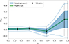 |
Fig. A.1. Weak-lensing bias for KiDS-1000 on eRASS1 clusters showing the calibration results on the simulation snapshots as black points and the interpolated trend as blue band (1σ uncertainty). At low redshift we are limited by the uncertainty on the multiplicative shear bias, while at higher redshift our uncertainty on the cluster member contamination dominates the systematic error budget (2σ uncertainties are indicated by the grey error-bars and light-blue curves). Hydro-dynamical modelling uncertainties, with 1σ uncertainties shown in green, remain sub-dominant. |
Multiplicative shear bias m and mean redshift offset Δz for the tomographic bins of KiDS-1000 from van den Busch et al. (2022).
We also modify the extraction model, by predicting a model for each tomographic bin according to its mean inverse critical surface mass density (compare Grandis et al. 2024, Eqn. 30). The resulting WL bias and scatter numbers are compressed into principal components which we report in Table A.2. We find that at low redshift the uncertainty on the multiplicative shear bias dominates the systematic error budget, while the dominating contribution comes from the estimate of the cluster member contamination at high redshift.
Calibration of the WL bias and scatter for KiDS-1000 WL on eRASS1 clusters.
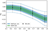 |
Fig. A.2. Weak-lensing bias of our extraction model on synthetic shear profile simulations reproducing the HSC WL signal around eRASS1 clusters and groups, showing the calibration results on the simulation snapshots as black points and the interpolated trend as blue band. Contrary to the DES WL bias, the depth of HSC permits a good background selection at all cluster redshifts considered. The larger shape measurement uncertainties however contribute to the WL bias uncertainty even when accounting for the systematics floor from hydro-dynamical modelling uncertainties (green band). |
Calibration of the WL bias and scatter for HSC WL on eRASS1 clusters.
A.2. WL mass bias for HSC S19
We also perform a weak-lensing bias and scatter determination for the HSC shear measurements, described in Ghirardini et al. (2024, Sect. 2.3.1). That analysis follows the same steps as Chiu et al. (2022). In our weak-lensing bias determination (see Grandis et al. 2024, Sect. 4) we introduce many modelling differences to the WL bias determination carried out in Chiu et al. (2022), Sect. 4.2. We therefore re-run the weak-lensing bias determination for HSC following the prescriptions made in this work. To account for the weak-lensing specifications of HSC we use
-
the calibrated source redshift distributions described in Chiu et al. (2022, Sect. 3.8),
-
the photo-z uncertainty described in the same section,
-
the same multiplicative shear bias uncertainty as employed in Chiu et al. (2022), and
-
the same upper limit on the cluster member contamination of < 6% that was derived in Chiu et al. (2022, Sect. 3.6).
After performing the extraction on many Monte Carlo realisations of the thusly created synthetic shear profiles, we derive the HSC weak-lensing bias shown in Fig. A.2. Contrary to the DES and KiDS WL bias uncertainty, the clean background selection implemented by Chiu et al. (2022), which is enabled by the extraordinary depth of the HSC data, makes the impact of photometric redshift uncertainties negligible. Instead, we find that uncertainties in the calibration of shape measurements contribute significantly to the uncertainty, even when compared to the current systematics floor given by the hydro-dynamical modelling.
Appendix B: Magnification and source number densities
Gravitational lenses cause magnification, which affects the number density of WL sources in several ways. To evaluate the impact thereof we closely follow Schrabback et al. (2018b, Sect. 6.7).
We use COSMOS2020 CLASSIC (Weaver et al. 2022) as a source catalogue that is complete up to KiDS-1000’s limiting magnitude. For simplification, we assumed that the COSMOS photo-zs roughly match those of KiDS-1000 such that we can divide COSMOS2020 into identical tomographic bins. We then calculated the lensing efficiency β(zi) of each galaxy i in the catalogue:
![Mathematical equation: $$ \begin{aligned} \beta (z_i)=\mathrm{max}\left[0,\,\frac{D_{\rm ls}}{D_{\rm s}}\right], \end{aligned} $$](/articles/aa/full_html/2025/03/aa49599-24/aa49599-24-eq48.gif) (B.1)
(B.1)
where Dls and Ds are the angular diameter distances from the lens to the source and to the source respectively. We choose a representative lens redshift of zcl = 0.2 for our testing. We approximate the magnification that every source experiences as
 (B.2)
(B.2)
where μ0, b is the magnification at an arbitrary fiducial lensing efficiency β0, b, for which we use the redshift centre of each tomographic bin (i.e. β0, b(z) = β0, b(0.6) for the tomographic bin 0.5 < zB ≤ 0.7).
Magnification can increase or decrease the source number density. It can increase it as it raises the brightness of sources according to
 (B.3)
(B.3)
This increase in brightness leads to fainter galaxies being detected that otherwise would not be included in the sample (we use the COSMOS2020 r-band magnitudes as the KiDS object detection relies on its respective r-band mosaics). On the other hand magnification increases the observed sky area, which leads to a dilution of the source number density by a factor 1/μ, for which we use μ0, b.
To keep track of both effects we calculate the magnification caused by an M500c = 2 × 10¹⁴ M⊙ NFW halo (at redshift 0.2) over the radial range of our analysis for each tomographic bin as
 (B.4)
(B.4)
where κ0, b(R) is the convergence of the NFW halo with respect to the fiducial lensing efficiency β0, b of each tomographic bin. Using these μ0, b we magnify the COSMOS2020 r-band magnitudes, calculate the relative change in galaxy number counts in magnitude bins, and convolve this profile with the tomographic r-band magnitude distributions of KiDS-1000. Together with the increase in observed sky area we obtain an approximate change in source number density for KiDS-1000. We show the result in Fig. B.1.
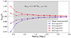 |
Fig. B.1. Calculated change in source number density in the different tomographic bins of KiDS-1000 for an NFW halo of mass M500c = 2 × 10¹⁴ M⊙, zcl = 0.2. In the low-redshift tomographic bins the increase in observed sky area (leading to a dilution of the source number density) dominates over the source number density increase due to fainter galaxies which move into the sample, whereas the opposite is the case for the high-redshift tomographic bins. |
We observe that magnification causes a decrease in source density for low-redshift tomographic bins (which are fairly complete in KiDS-1000), as the dilution of the source density dominates over the gain due to the increased source brightnesses. The opposite is the case for the high-redshift tomographic bins, for which KiDS-1000 probes the brighter and steeper part of the galaxy luminosity function. Generally the effect is around the one percent level, except for small cluster centric distances, depending on the tomographic bin. We note that our approximation does not account for the additional second-order effect that the increased source sizes may have on the lensing weights.
Together with the fact that magnification has opposite effects in different tomographic bins (which partly cancel from the perspective of a systematic halo mass bias) and that an accurate convergence profile, and therefore halo mass, is necessary to employ a correction, this leads us to dismiss the effect in our analysis. However, we note that one will need to account for magnification in analyses of upcoming stage-IV WL surveys (which aim to reach percent level accuracy), if they rely on source number densities to assess cluster member contamination.
Appendix C: Acknowledgements
We like to thank Prof. Dr. Henk Hoekstra and Dr. Angus H. Wright for their useful feedback on the manuscript draft.
The KiDS-1000 data products are based on observations made with ESO Telescopes at the La Silla Paranal Observatory under programme IDs 177.A-3016, 177.A-3017, 177.A-3018 and 179.A-2004, and on data products produced by the KiDS consortium. The KiDS production team acknowledges support from: Deutsche Forschungsgemeinschaft, ERC, NOVA and NWO-M grants; Target; the University of Padova, and the University Federico II (Naples).
F. Kleinebreil, S. Grandis, and T. Schrabback acknowledge support from the German Federal Ministry for Economic Affairs and Energy (BMWi) provided through DLR under projects 50OR2002, 50OR2106, and 50OR2302, support provided by the Deutsche Forschungsgemeinschaft (DFG, German Research Foundation) under grant 415537506, as well as support provided by the Austrian Research Promotion Agency (FFG) and the Federal Ministry of the Republic of Austria for Climate Action, Environment, Mobility, Innovation and Technology (BMK) via the Austrian Space Applications Programme with grant numbers 899537 and 900565.
This work is based on data from eROSITA, the soft X-ray instrument aboard SRG, a joint Russian-German science mission supported by the Russian Space Agency (Roskosmos), in the interests of the Russian Academy of Sciences represented by its Space Research Institute (IKI), and the Deutsches Zentrum für Luft und Raumfahrt (DLR). The SRG spacecraft was built by Lavochkin Association (NPOL) and its subcontractors and is operated by NPOL with support from the Max Planck Institute for Extraterrestrial Physics (MPE).
The development and construction of the eROSITA X-ray instrument was led by MPE, with contributions from the Dr. Karl Remeis Observatory Bamberg & ECAP (FAU Erlangen-Nuernberg), the University of Hamburg Observatory, the Leibniz Institute for Astrophysics Potsdam (AIP), and the Institute for Astronomy and Astrophysics of the University of Tübingen, with the support of DLR and the Max Planck Society. The Argelander Institute for Astronomy of the University of Bonn and the Ludwig Maximilians Universität Munich also participated in the science preparation for eROSITA.
The eROSITA data shown here were processed using the eSASS software system developed by the German eROSITA consortium.
V. Ghirardini, E. Bulbul, A. Liu, C. Garrel, and X. Zhang acknowledge financial support from the European Research Council (ERC) Consolidator Grant under the European Union’s Horizon 2020 research and innovation program (grant agreement CoG DarkQuest No 101002585). N. Clerc was financially supported by CNES.
The Legacy Surveys consist of three individual and complementary projects: the Dark Energy Camera Legacy Survey (DECaLS; Proposal ID #2014B-0404; PIs: David Schlegel and Arjun Dey), the Beijing-Arizona Sky Survey (BASS; NOAO Prop. ID #2015A-0801; PIs: Zhou Xu and Xiaohui Fan), and the Mayall z-band Legacy Survey (MzLS; Prop. ID #2016A-0453; PI: Arjun Dey). DECaLS, BASS and MzLS together include data obtained, respectively, at the Blanco telescope, Cerro Tololo Inter-American Observatory, NSF’s NOIRLab; the Bok telescope, Steward Observatory, University of Arizona; and the Mayall telescope, Kitt Peak National Observatory, NOIRLab. Pipeline processing and analyses of the data were supported by NOIRLab and the Lawrence Berkeley National Laboratory (LBNL). The Legacy Surveys project is honored to be permitted to conduct astronomical research on Iolkam Du’ag (Kitt Peak), a mountain with particular significance to the Tohono O’odham Nation.
Funding for the DES Projects has been provided by the U.S. Department of Energy, the U.S. National Science Foundation, the Ministry of Science and Education of Spain, the Science and Technology Facilities Council of the United Kingdom, the Higher Education Funding Council for England, the National Center for Supercomputing Applications at the University of Illinois at Urbana-Champaign, the Kavli Institute of Cosmological Physics at the University of Chicago, the Center for Cosmology and Astro-Particle Physics at the Ohio State University, the Mitchell Institute for Fundamental Physics and Astronomy at Texas A&M University, Financiadora de Estudos e Projetos, Fundação Carlos Chagas Filho de Amparo à Pesquisa do Estado do Rio de Janeiro, Conselho Nacional de Desenvolvimento Científico e Tecnológico and the Ministério da Ciência, Tecnologia e Inovação, the Deutsche Forschungsgemeinschaft, and the Collaborating Institutions in the Dark Energy Survey.
The Collaborating Institutions are Argonne National Laboratory, the University of California at Santa Cruz, the University of Cambridge, Centro de Investigaciones Energéticas, Medioambientales y Tecnológicas-Madrid, the University of Chicago, University College London, the DES-Brazil Consortium, the University of Edinburgh, the Eidgenössische Technische Hochschule (ETH) Zürich, Fermi National Accelerator Laboratory, the University of Illinois at Urbana-Champaign, the Institut de Ciències de l’Espai (IEEC/CSIC), the Institut de Física d’Altes Energies, Lawrence Berkeley National Laboratory, the Ludwig-Maximilians Universität München and the associated Excellence Cluster Universe, the University of Michigan, the National Optical Astronomy Observatory, the University of Nottingham, The Ohio State University, the OzDES Membership Consortium, the University of Pennsylvania, the University of Portsmouth, SLAC National Accelerator Laboratory, Stanford University, the University of Sussex, and Texas A&M University.
The Hyper Suprime-Cam (HSC) collaboration includes the astronomical communities of Japan and Taiwan, and Princeton University. The HSC instrumentation and software were developed by the National Astronomical Observatory of Japan (NAOJ), the Kavli Institute for the Physics and Mathematics of the Universe (Kavli IPMU), the University of Tokyo, the High Energy Accelerator Research Organization (KEK), the Academia Sinica Institute for Astronomy and Astrophysics in Taiwan (ASIAA), and Princeton University. Funding was contributed by the FIRST program from the Japanese Cabinet Office, the Ministry of Education, Culture, Sports, Science and Technology (MEXT), the Japan Society for the Promotion of Science (JSPS), Japan Science and Technology Agency (JST), the Toray Science Foundation, NAOJ, Kavli IPMU, KEK, ASIAA, and Princeton University.
This paper makes use of software developed for Vera C. Rubin Observatory. We thank the Rubin Observatory for making their code available as free software at http://pipelines.lsst.io/.
This paper is based on data collected at the Subaru Telescope and retrieved from the HSC data archive system, which is operated by the Subaru Telescope and Astronomy Data Center (ADC) at NAOJ. Data analysis was in part carried out with the cooperation of Center for Computational Astrophysics (CfCA), NAOJ. We are honored and grateful for the opportunity of observing the Universe from Maunakea, which has the cultural, historical and natural significance in Hawaii.
The Pan-STARRS1 Surveys (PS1) and the PS1 public science archive have been made possible through contributions by the Institute for Astronomy, the University of Hawaii, the Pan-STARRS Project Office, the Max Planck Society and its participating institutes, the Max Planck Institute for Astronomy, Heidelberg, and the Max Planck Institute for Extraterrestrial Physics, Garching, The Johns Hopkins University, Durham University, the University of Edinburgh, the Queen’s University Belfast, the Harvard-Smithsonian Center for Astrophysics, the Las Cumbres Observatory Global Telescope Network Incorporated, the National Central University of Taiwan, the Space Telescope Science Institute, the National Aeronautics and Space Administration under grant No. NNX08AR22G issued through the Planetary Science Division of the NASA Science Mission Directorate, the National Science Foundation grant No. AST-1238877, the University of Maryland, Eotvos Lorand University (ELTE), the Los Alamos National Laboratory, and the Gordon and Betty Moore Foundation.
This work made use of the following Python software packages: NumPy7 (Harris et al. 2020), SciPy8 (Virtanen et al. 2020), Matplotlib9 (Hunter 2007), Astropy10 (Astropy Collaboration 2022).
All Tables
Sample averaged differences in the amplitudes of scaled isothermal sphere shear profiles relative to the uncertainty of the differences measured in DES and HSC with regard to KiDS estimates based on different tomographic redshift bins.
Calibration of the count rate to halo mass relation parameters for eROSITA using different weak-lensing data sets and cluster samples.
Multiplicative shear bias m and mean redshift offset Δz for the tomographic bins of KiDS-1000 from van den Busch et al. (2022).
All Figures
|
Fig. 1. Footprint of KiDS-1000 North (top) and South (bottom) as well as DES Y3 (overlap with KiDS South), HSC S19 (overlap with KiDS North), and the eRASS1 cluster sample. |
| In the text | |
|
Fig. 2. Five spectroscopically calibrated tomographic redshift bins of KiDS. The redshift resolution is 0.05. We colour-coded the low-redshift tomographic bins blue and the high-redshift bins red, a convention that we preserve throughout this work. |
| In the text | |
|
Fig. 3. Richness and redshift distribution of the eRASS1 clusters located in the KiDS-1000 footprint. Also included is a division into sub-samples for the tests presented in Sect. 3.2. |
| In the text | |
|
Fig. 4. Exemplary radial tangential reduced shear profile of the eRASS1 cluster em01_019120_020_ML00027_002_c947 in KIDS-1000 with a cluster redshift zcl = 0.16. We measured the shear separately in the tomographic background photo-z bins and plot the data points at the average projected radius of the contributing galaxies. |
| In the text | |
|
Fig. 5. Annuli around the cluster centres can have varying contributions from different tiles of the KiDS mosaic. Left: Exemplary cluster field the of eRASS1 cluster em01_019120_020_ML00027_002_c947, which covers four KiDS pointings. The grey areas are masked in KiDS-1000. Right: Fraction of unmasked area that each pointing contributes to a given annulus and fraction of masked pixels. |
| In the text | |
|
Fig. 6. Exemplary weighted & normalised radial number density profile for the eRASS1 cluster em01_046120_020_ML00096_002_c947 in KiDS-1000 with zcl = 0.25, λ = 50.9, uncorrected for obscuration. One can observe an increase in the normalised source density for the low-redshift tomographic bin towards the cluster centre due to cluster member contamination. The high-redshift tomographic bins show a decrease in source density due to obscuration from cluster galaxies. The bottoms panel shows the corresponding varying reference number density (weighted with lensing weights). |
| In the text | |
|
Fig. 7. Exemplary weighted radial detection probability profile of the eRASS1 cluster em01_022120_020_ML00040_002_c947. The bottom panel shows the corresponding varying reference detection probability (weighted with lensing weights). |
| In the text | |
|
Fig. 8. Best-fit parameters of the redshift evolution of the object detection bias from the global fit of all individual radial detection profiles. |
| In the text | |
|
Fig. 9. Measured and best-fit radial detection profiles stacked separately for the different tomographic source bins (panels) and divided into three cluster sub-samples. |
| In the text | |
|
Fig. 10. Best-fit result of the amplitude parameter of the global contamination model at pivot points in the cluster redshift space. Bottom: Distribution of the eRASS1 KiDS-1000 cluster redshifts. |
| In the text | |
|
Fig. 11. Measured and best-fit detection-corrected radial number density profiles stacked in tomographic bins (different panels) and divided into three cluster sub-samples. We employed inverse-variance weighting to take the average at each radius, which pronounces clusters as scattering low. |
| In the text | |
|
Fig. 12. Best-fit contamination model for richness 15 and 80 at a cluster-centric distance of 1 Mpc as a function of the cluster redshift and always showing the lowest included tomographic source bin only. Here, we set amplitude parameters f′(zcl) that scatter to negative values to zero, which mirrors the treatment of the contamination model in Appendix A.1. |
| In the text | |
|
Fig. 13. Consistency test between the density contrast profiles of clusters observed both in DES (HSC) and KiDS in the upper (lower) panels. Given the correlated intrinsic galaxy shapes, we constructed the statistical uncertainty estimates by bootstrapping on the union of the respective source catalogues. We find that, averaged over all objects, the estimates from the survey pairs are consistent as a function of radius (left column). Also, the uncertainty weighted mean square deviation of all clusters, shown in the right column, is consistent with the expectation (red curve). |
| In the text | |
|
Fig. 14. Difference in the amplitude of the isothermal sphere shear profile models fitted to clusters with coverage by DES and KiDS (HSC and KiDS) in the left (right) panel plotted relative to the uncertainty of this difference and as a function of cluster redshift and richness (columns) for the different KiDS tomographic redshift bins (rows). We found excellent overall agreement, while no richness or redshift trends are evident from visual inspection, also after binning (black points). |
| In the text | |
|
Fig. 15. One- and two-dimensional marginal contour plots for the WL mass calibration of the eROSITA count rate to halo mass relation. In green the results from KiDS-1000 on eRASS1 are shown, in blue are the results from DES Y3 on eRASS1 (Grandis et al. 2024), in orange are the results from HSC-Y3 on eRASS1, and in black are the results from HSC-Y3 on eFEDS (Chiu et al. 2022). All results show agreement, indicating the reliability of the WL mass calibration methods employed by the different teams. |
| In the text | |
|
Fig. 16. Stacked tangential reduced shear profiles from KiDS-1000 for different tomographic redshift bins (rows) and cluster redshift bins (columns) together with the mean stacked model and its one sigma uncertainty (filled area). The mean stacked model incorporates the model for cluster member contamination, making the model prediction and the data directly comparable. The model fits the data very well. |
| In the text | |
|
Fig. 17. Stacked tangential reduced shear profiles measured using the HSC data and split according to cluster count rate (rows) and cluster redshift bins (columns) together with the mean stacked model and its one sigma uncertainty (filled area). Not all the stacked reduced shear profiles result in statistically good fits (especially at low count rates), leading to a rather high χ2. |
| In the text | |
|
Fig. A.1. Weak-lensing bias for KiDS-1000 on eRASS1 clusters showing the calibration results on the simulation snapshots as black points and the interpolated trend as blue band (1σ uncertainty). At low redshift we are limited by the uncertainty on the multiplicative shear bias, while at higher redshift our uncertainty on the cluster member contamination dominates the systematic error budget (2σ uncertainties are indicated by the grey error-bars and light-blue curves). Hydro-dynamical modelling uncertainties, with 1σ uncertainties shown in green, remain sub-dominant. |
| In the text | |
|
Fig. A.2. Weak-lensing bias of our extraction model on synthetic shear profile simulations reproducing the HSC WL signal around eRASS1 clusters and groups, showing the calibration results on the simulation snapshots as black points and the interpolated trend as blue band. Contrary to the DES WL bias, the depth of HSC permits a good background selection at all cluster redshifts considered. The larger shape measurement uncertainties however contribute to the WL bias uncertainty even when accounting for the systematics floor from hydro-dynamical modelling uncertainties (green band). |
| In the text | |
|
Fig. B.1. Calculated change in source number density in the different tomographic bins of KiDS-1000 for an NFW halo of mass M500c = 2 × 10¹⁴ M⊙, zcl = 0.2. In the low-redshift tomographic bins the increase in observed sky area (leading to a dilution of the source number density) dominates over the source number density increase due to fainter galaxies which move into the sample, whereas the opposite is the case for the high-redshift tomographic bins. |
| In the text | |
Current usage metrics show cumulative count of Article Views (full-text article views including HTML views, PDF and ePub downloads, according to the available data) and Abstracts Views on Vision4Press platform.
Data correspond to usage on the plateform after 2015. The current usage metrics is available 48-96 hours after online publication and is updated daily on week days.
Initial download of the metrics may take a while.