© The Authors 2024

1. Introduction

General relativity describes the gravitational force as the curvature of space-time induced by mass and energy densities. This curvature determines the so-called null geodesics on which photons travel through space-time. As a consequence, the path of the light from a distant source to the observer is deflected by intervening gravitational potentials, with a deflection angle that is proportional to the path integral of the transverse component of the negative gradient of the potential. Indeed, Dyson et al. (1920) measured the predicted displacement in the positions of distant stars when observed close to the Sun during a solar eclipse. In the cosmological context, the original position of the sources is not known. In general, the gravitational potential of the intervening lenses is also unknown because the majority of cosmic matter is believed to be invisible, and its density is among the targets of our experiments.

On cosmic scales, gravitational lensing of distant galaxies thus relies on the fact that the differential deflection of neighboring light paths locally induces a magnification and a distortion of the source galaxy image (for a pedagogical introduction see Schneider 2006). In this regime, large-scale gravitational potentials create spatially coherent, small distortions in the observed shapes of background galaxies, a process called weak gravitational lensing (hereafter WL). A special case is the WL caused by massive gravitationally collapsed, virialized structures, referred to as halos, which dominate the line-of-sight-integrated gravitational potential (for a review see Umetsu 2020). These objects induce a tangential distortion in the shapes of the background galaxies, that traces the density contrast of the 2D projected density profiles. The 3D density profiles of halos are well understood in simulations and are found to tightly follow a parametric class of functions with two free parameters: the total halo mass and the typical halo scale (Navarro et al. 1996). Fitting predictions derived from this family of models to the tangential reduced shear profiles thus enables the direct measurement of the halo mass.0]Please note that e-mail mismatch found between SAGA and Tex file. We followed Tex file.

The most massive halos host galaxy clusters, whose observed properties display tight correlations among themselves (Mohr & Evrard 1997), and with the host halos mass (Angulo et al. 2012), enabling a clean halo selection. For such samples of galaxy clusters, the WL mass information is then used to reconstruct the differential number density of halos as a function of mass and redshift, the halo mass function. This function traces the growth of the structure in the Universe and is therefore a sensitive probe to the total matter density, the accelerated expansion, and gravity itself (Haiman et al. 2001; Majumdar & Mohr 2004; Allen et al. 2011). Examples of such analyses are Mantz et al. (2015), who used X-ray-selected galaxy clusters with pointed WL observations, and Bocquet et al. (2019), who used galaxy clusters selected at millimeter wavelengths. Both of these analyses resulted in competitive cosmological constraints, which are largely complementary and independent of other cosmological probes (for a recent review, see Huterer 2023).0]Please note that the affiliations “5, 54, 63 and 64” are provided in the affiliations list but not designated with any authors in the author group. Please provide the citations or delete them from the affiliations list.

Our ability to detect larger numbers of massive halos has recently been transformed by eROSITA, which performed its first all-sky survey from December 2019 to June 2020 (Predehl et al. 2021; Sunyaev et al. 2021), detecting more than 1 million X-ray sources in the Western Galactic Hemisphere (Merloni et al. 2024). Among these X-ray sources, ∼12 k are confirmed as clusters of galaxies through significant extended X-ray emission and associated red galaxy members in the 12791 deg² footprint covered by the DESI Legacy Survey DR9 and DR10 data (Bulbul et al. 2024; Kluge et al. 2024). In this work, we restricted ourselves to the 5263 clusters selected for the cosmology sample via a higher extent likelihood cut. These clusters have percent-accurate photometric redshifts, in the range of 0.1–0.8, and a well calibrated selection function (Clerc et al. 2024).0]Please note that the author “M. Smith” is designated with affiliation “69”, but the corresponding affiliation has not provided in the affiliations list. Please include this in the affiliations list or remove the designator.

We complement the eROSITA data with the wide photometric Dark Energy Survey year 3 (DES Y3) data (Sevilla-Noarbe et al. 2021). From these data, we used more than 10⁸ galaxy shape measurements measured in the riz bands by Gatti et al. (2021) in an effective survey area of 4143 deg² of the southern sky. The strength of the WL signal around galaxy clusters depends not only on their mass but also on the geometrical configuration of the lens and source. To statistically estimate the latter’s distance, we leveraged the exquisite accuracy of the photometric redshift calibration of the DES Y3 sources by Myles et al. (2021).

Besides the uncertainty on the shape and photometric redshift measurements for the source galaxies, percent-accurate cluster WL measurements need to account for the cluster mis-centering errors and contamination of the source sample by cluster galaxies (for a complete analysis on DES year 1 data, see McClintock et al. 2019). Even if all observational systematics are well calibrated and accounted for, the modeling uncertainties of baryonic feedback processes alter the mass distribution of galaxy clusters. This poses a theoretical limit to our ability to calibrate cluster masses via WL (Grandis et al. 2021a). As argued in that work, setting up many realizations of realistic, synthetic cluster WL mock datasets and analyzing them with the same mass extraction method as the real data allows one to calibrate both the absolute values and – crucially – the uncertainty of the WL mass bias. This approach has already been successfully demonstrated in work by Chiu et al. (2022) in the context of Hyper Supreme Camera (HSC) observations of the eROSITA Final Equatorial-Depth Survey (eFEDS) used for science verification.

This paper is organized as follows: In Sect. 2, we describe the lens and source catalogs, as well as the calibration products used in this analysis. Section 3 then describes the measurement process for the tangential reduced shear and the suite of associated validation and calibration steps. In Sect. 4, we then describe the shear profile model used for the mass measurement, as well as its calibration on realistic synthetic data. These two sections follow in significant part the analysis performed by Bocquet et al. (2023) of the DES Y3 WL signal around South Pole Telescope (SPT) selected clusters. The actual mass calibration is then performed and validated in Sect. 5, and we discuss our results in Sect. 6. Halo masses in this work are reported as spherical over density masses M_Δc, with Δ = 500, 200. This means that they are defined via the radius R_Δc enclosing a sphere of average density Δ times the critical density of the Universe at that redshift, that is, $M_{\mathrm{\Delta }\mathrm{c}}=\frac{4\pi }{3}\mathrm{\Delta }{\rho }_{\mathrm{crit}}(z)R_{\mathrm{\Delta }\mathrm{c}}^3$. We used a flat ΛCDM cosmology with the parameters Ω_M = 0.3, and h = 0.7 as the reference cosmology, where not specified otherwise. Throughout this work, we use lens redshift z_l, and cluster redshift z_cl interchangeably, depending on which is more applicable to the context of the discussion.

2. Data

2.1. eRASS1 cluster and group sample

As a lens catalog, we use the cluster catalog acquired from the first eROSITA All-Sky Survey on the Western Galactic Hemisphere, completed on June 11, 2020. The detection properties of the X-ray sources detected in this survey, including extended sources, are discussed in detail in Merloni et al. (2024), Bulbul et al. (2024). We use the cosmology catalog described in detail in Bulbul et al. (2024), comprised of X-ray sources detected as significantly extended, with reliable photometric confirmation and redshift estimation using the DESI Legacy Survey DR10 (Dey et al. 2019). Specifically, Kluge et al. (2024) run an adapted version of the redMaPPer algorithm (Rykoff et al. 2014, 2016; Rozo et al. 2015) on the X-ray cluster candidate position, thus measuring their richness and photometric redshift. Of the 5263 clusters and groups in that catalog, 2201 have DES Y3 shape and photo-z information (described below), and are therefore used for the WL analysis in this work (see Ghirardini et al. 2024, Fig. 1 for a comparison of the two survey footprints). Their distribution in redshift, richness and X-ray photon count rate is shown in Fig. 1. The bulk of the lens sample lies at low redshift, ideally placed for WL studies. Some objects at low richness have redshifts much larger than expected for an X-ray-selected sample. We account for these contaminants in our mass calibration (see Sect. 5.1.1).

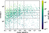Fig. 1. Lens sample composed of the eRASS1 cosmology cluster and group sample with DES WL data, plotted in redshift against richness and with the X-ray count rate color coded. The gray lines mark the edges of the richness–redshift bins used for the calibration and validation of the WL measurement. Cosmology ready WL data products are, however, produced for each cluster individually.

2.2. DES WL data

The Dark Energy Survey is an approximately 5000 deg² photometric survey in the optical bands grizY, carried out at the 4 m Blanco telescope at the Cerro Tololo Inter-American Observatory (CTIO), Chile, with the Dark Energy Camera (DECam Flaugher et al. 2015). In this analysis, we utilize data from the first three years of observations (DES Y3), covering the full survey footprint.

2.2.1. The shape catalog

The DES Y3 shape catalog (Gatti et al. 2021) is built from the r, i, z-bands using the METACALIBRATION pipeline (Huff & Mandelbaum 2017; Sheldon & Huff 2017). Other DES Y3 publications contain more detailed information about the photometric dataset (Sevilla-Noarbe et al. 2021), the Point-Spread Function modeling (Jarvis et al. 2021), and image simulations (MacCrann et al. 2022). We refer the reader to these works for more information. After applying all source selection cuts, the DES Y3 shear catalog contains about 100 million galaxies over an area of 4143 square degrees. Its effective source density is 5–6 arcmin⁻², depending on the exact definition. In Sect. 3, we will derive the exact values of effective source density.

2.2.2. Source redshift distributions and shear calibration

Our analysis uses the same selection of lensing source galaxies in tomographic bins as the DES 3 × 2pt analysis (Dark Energy Survey Collaboration 2022). This selection is defined in Myles et al. (2021). In that work, source redshifts are estimated with Self-Organizing Maps, and the method is thus referred to as SOMPz. The final calibration accounts for the (potentially correlated) systematic uncertainties in source redshifts and shear measurements, as determined in the image simulations by MacCrann et al. (2022). For each tomographic source bin b, the estimated redshift distribution P_ℋ(z_s|b) is provided, and the systematic uncertainties on this estimate are captured through 1000 realizations (see Fig. 2). These realizations are indexed via the hyperparameter ℋ, which takes integer values between 0 and 999 (Cordero et al. 2022). For convenience, these redshift distributions are normalized to varying values (1 + m), where the varying m spans the range of the multiplicative shear bias values. Note that the DES Y3 survey only has minor depth variations over the survey area. The survey averaged quantities, like the source redshift distributions, thus apply to the joint eROSITA-DE – DES Y3 footprint.

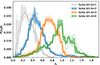Fig. 2. Source redshift distributions of the tomographic redshift bin of the DES Y3 data. We plot the mean of the 1000 realizations (full line), together with the 16–84 percentile (filled region) and the 2.5–97.5 percentile (faded lines). The first tomographic bin is not used, while the others are weighted to ensure a lens-dependent background selection.

We will also use DNF (De Vicente et al. 2016) and BPZ (Benítez 2000) source redshift measurements to constrain the amount of cluster member contamination in our source sample (see Sect. 3.3.1). While BPZ is a Bayesian template fitting code, DNF is based on a nearest-neighbor interpolation on the color-magnitude space of spectroscopic reference samples. As such, BPZ is more robust against the incompleteness of the spectroscopic reference samples, while DNF is more data-driven and avoids the biases that occur from the template choice (see Sevilla-Noarbe et al. 2021, Sect. 6.3, for more details).

3. Measurement

In this section, we shall outline (1) the methods used to measure the WL signal around eROSITA selected clusters, (2) the steps undertaken to calibrate this measurement correctly, and (3) the use of this measurement to determine the mass scale of the eROSITA selected clusters and groups. Note that the methods presented in this work draw significantly upon those presented in Bocquet et al. (2023).

3.1. WL by massive halos

Assuming that background galaxies are isotropically oriented intrinsically, the coherent tangential distortion induced by the gravitational potential on background galaxy images at a radius R from the halo center can be obtained, to linear order, by averaging the tangential component of their ellipticities,

$$\begin{array}{c}\hfill g_{\mathrm{t}}(R)={\mathcal{R}}^{-1}{⟨e_{\mathrm{t}}⟩}_R,\end{array}$$(1)

where g_t(R) is the reduced tangential reduced shear, and ℛ is the average response of the measured ellipticity to a shear (shear response). In practical applications, instrumental effects and noise make it different from 1. It is determined through galaxy shape measurement and validated through image simulations. Below, we discuss how we include this effect in our measurements and how we account for nonlinear responses. While the ellipticity field itself is not Gaussian, our reduced shear estimator is constructed by averaging many sources. The central limit theorem thus ensures that the statistical error of the shear estimate can be directly derived from the effective dispersion σ_eff in the ellipticity of the source galaxies and their effective number N_eff. Below, we will discuss how we estimate these two quantities.

Given a source galaxy at redshift z_s, the lens redshift z_l, and the surface mass density Σ(x) in the lens plane, the tangential reduced shear in any position on the sky θ = x/D_l is given by

$$\begin{array}{c}\hfill g_{\mathrm{t}}(\mathit{\theta })=\frac{{\gamma }_{\mathrm{t}}(\mathit{x})}{1-\kappa (\mathit{x})}\mathrm{with}\kappa (\mathit{x})={\mathrm{\Sigma }}_{\mathrm{crit}}^{-1}\mathrm{\Sigma }(\mathit{x}),\end{array}$$(2)

where γ_t(x) is the tangential component of the shear, κ(x) the convergence, D_l the angular diameter distance to the lens, and ${\mathrm{\Sigma }}_{\mathrm{crit}}^{-1}$ the inverse of the critical lensing surface density. The latter expresses the geometrical configuration of the source and lens and is given by

$$\begin{array}{c}\hfill {\mathrm{\Sigma }}_{\mathrm{crit},\mathrm{ls}}^{-1}=\frac{4\pi G}{c^2}\frac{D_{\mathrm{l}}}{D_{\mathrm{s}}}max[0,D_{\mathrm{ls}}],\end{array}$$(3)

where G is the gravitational constant, c the speed of light. Furthermore, we use the angular diameter distance between observer and source (D_s), and lens and source (D_ls). Note that for sources in front of the lens, D_ls becomes negative. These sources are not lensed, which we account for by setting their inverse critical lensing surface density to zero. Hence the term max[0,D_ls].

In general relativity, the azimuthally averaged tangential shear at projected radius R is proportional to the density contrast,

$$\begin{array}{c}\hfill {\gamma }_{\mathrm{t}}(R)={\mathrm{\Sigma }}_{\mathrm{crit}}^{-1}[⟨\mathrm{\Sigma }(<R)⟩-\mathrm{\Sigma }(R)],\end{array}$$(4)

while the orthogonal, B-mode-like component γ_x, called cross-shear (see below for the exact definition of the decomposition), averages to zero when integrated over closed paths such as radial bins,

$$\begin{array}{c}\hfill {\gamma }_{\mathrm{x}}(R)=0.\end{array}$$(5)

We will use the latter as a validation test for our measurement.

3.2. Measurement

To perform the measurement, for each lens l, we query the shape catalog for all sources at a projected physical distance of < 15 h⁻¹ Mpc in the reference cosmology (h = 0.7, Ω_M = 0.3). For each source lens pair (i, l), we compute the position angle φ at which the source is seen from the lens’ position.

We then project the ellipticity components e_1, 2 onto the tangential and cross components as

$$\begin{array}{cc}& e_{\mathrm{t}}=-e_{1}cos2\phi +e_{2}sin2\phi \hfill \\ \hfill & e_{\mathrm{x}}=e_{1}sin2\phi +e_{2}cos2\phi .\hfill \end{array}$$(6)

We use the tangential/cross decomposition for the case where the e₂-component is defined with respect to right ascension, which is the case in the DES Y3 shape catalog¹ We also record the source weight $w_i^s$, and the photometric redshift estimates in the form of the SOMPz cell c_SOM, i of the source, and the photometric redshift estimates ${\widehat{z}}_{\mathrm{D}\mathrm{N}\mathrm{F},i}$ and ${\widehat{z}}_{\mathrm{B}\mathrm{P}\mathrm{Z},i}$. Furthermore, we compute the response ℛ_i of every single source by interpolating the response as a function of size with respect to to the PSF and signal-to-noise, as presented in the upper right panel of Fig. 4 in Gatti et al. (2021), Sect. 4.3.

To select only sources in the background of each lens, we discard the first tomographic redshift bin and apply a weight to each source depending on the tomographic redshift bin b it resides in,

$$\begin{array}{c}\hfill w^b=\{\begin{array}{cc}{\langle {\mathrm{\Sigma }}_{\mathrm{crit},\mathrm{ls}}^{-1}\rangle }_{\mathrm{s}\in b}\hfill & \mathrm{for}{z}_{\mathrm{l}}<z_{\mathrm{med},b}\mathrm{and}b>1\hfill \\ 0.\hfill & \mathrm{otherwise},\hfill \end{array}\end{array}$$(7)

where the average is taken using the mean source redshift distribution of the tomographic bin, as reported by Myles et al. (2021). Our background selection is thus a weighted sum of the tomographic bin selections. This is convenient, as the shear and photo-z calibration (Myles et al. 2021; Cordero et al. 2022; MacCrann et al. 2022) is only valid for the specific selection criteria of the tomographic redshift bins. It can be extended to our analysis by using the same weights as above. Our selection excludes the 2nd tomographic redshift bins for z_l > 0.47, and the third for z_l > 0.74.

To validate and calibrate the cluster WL measurement, we define lens richness bins (3, 16, 26, 38, 55, 250), and redshift bins (0.10, 0.19, 0.27, 0.35, 0.48, 0.8), shown as gray lines in Fig. 1, and tuned to result in approximately even occupations of the lenses. In these bins, we measure the following quantities for radial bins whose upper edges are log-equally spaced between 0.2–15 h⁻¹ Mpc at the lens redshift in the reference cosmology:

• the raw tangential and cross-shear, with the tangential components shown in Fig. 3,

  $$\begin{array}{c}\hfill g_{\alpha ,\mathrm{raw}}=\frac{{\sum }_{b=2,3,4}{w}^b{\sum }_{i\in b}{w}_i^{\mathrm{s}}{e}_{\alpha ,i}}{{\sum }_{b=2,3,4}{w}^b{\sum }_{i\in b}{w}_i^{\mathrm{s}}{\mathcal{R}}_i}\mathrm{for}\alpha \in (t,x),\end{array}$$(8)

  where i ∈ b stands for the source i in the tomographic bin b and in the respective lens richness, redshift, and distance bins.

• the effective number of sources

  $$\begin{array}{c}\hfill N_{\mathrm{eff}}=\frac{{\left({\sum }_{b=2,3,4}{\sum }_{i\in b}{w}^b{w}_i^{\mathrm{s}}{\mathcal{R}}_i\right)}^2}{{\sum }_{b=2,3,4}{\sum }_{i\in b}{\left(w^b{w}_i^{\mathrm{s}}{\mathcal{R}}_i\right)}^2},\end{array}$$(9)

• the effective dispersion of source ellipticities

  $$\begin{array}{c}\hfill {\sigma }_{\alpha ,\mathrm{eff}}^2=\frac{{\sum }_{b=2,3,4}{\sum }_{i\in b}{\left(w^b{w}_i^{\mathrm{s}}\right)}^2{e}_{\alpha ,b,i}^2}{{\sum }_{b=2,3,4}{\sum }_{i\in b}{\left(w^b{w}_i^{\mathrm{s}}{\mathcal{R}}_i\right)}^2}\mathrm{for}\alpha \in (t,x),\mathrm{and}\end{array}$$(10)

• the source redshift distribution for fine source redshift bins with edges (z_s−, z_s+), reading

  $$\begin{array}{c}\hfill {\widehat{P}}_{\beta }(z_s)=\frac{{\sum }_{b=2,3,4}{w}^b{\sum }_{i\in b}{w}_i^{\mathrm{s}}{\mathcal{R}}_i{\mathrm{I}}_s({\widehat{z}}_{\beta ,i})}{{\sum }_{b=2,3,4}{w}^b{\sum }_{i\in b}{w}_i^{\mathrm{s}}{\mathcal{R}}_i}\mathrm{for}\beta \in (\mathit{bpz},\mathit{dnf}),\end{array}$$(11)

  where ${\mathrm{I}}_s({\widehat{z}}_{\beta ,i})=1$ when $z_{\mathrm{s}-}<{\widehat{z}}_{\beta ,i}<z_{\mathrm{s}+}$. Practically speaking, this is a weighted histogram of the photo-z estimates ${\widehat{z}}_{\beta ,i}$.

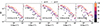Fig. 3. Absolute value of the raw tangential reduced shear profile, Eq. (8), in bins of cluster redshift (panels: lowest redshift left, higher redshift right) and of richness (color coding), for our background selection. Stars denote positive values, while empty circles denote negative values. The profiles show a clear increase toward the cluster centers, as well as a trend with richness, in line with our qualitative expectations.

It is important to note that also the estimates of the effective source density, the shape dispersion and the redshift distribution need to take the shear response ℛ into account. For a derivation for Eqs. (9) and (10), we refer the reader to Appendix A, where we present the derivation of the effective number of sources and their effective shape dispersion in the presence of a shear response and un-normalized weights.

3.3. Calibration and validation

We shall now discuss several calibration and validation steps we take to ensure the quality of our WL measurements.

3.3.1. Cluster member contamination

As suggested by their name, galaxy clusters are substantial over-densities not only in matter but also in the galaxy field. As a result, an a priori unknown fraction of the cluster members contaminates any source background selection. These cluster member contaminants carry no shear distortion signal from the cluster potential and therefore dilute the shear signal (Hoekstra et al. 2012; Gruen et al. 2014; Dietrich et al. 2019; Varga et al. 2019). This effect is equivalent to source-lens clustering in other WL applications (compare, for instance, with Prat et al. 2022, Sect. III.B). Current simulations are not accurate enough to reconstruct the colors and magnitudes of cluster member galaxies with sufficient fidelity to calibrate this effect directly in simulations. We therefore resorted to empirical calibration methods. We shall outline in the following paragraphs the model for the cluster member contamination, and the two methods we use to fit for it, as well as a comparison of the fit results.

Cluster member contamination model. In modeling the cluster member contamination, we adopt an approach that was developed previously in Paulus (2021). We parametrize the radial fraction of cluster contaminants as

$$\begin{array}{cc}& f_{\mathrm{cl}}(R|\lambda ,z)=\frac{A(\lambda ,z,R)}{1+A(\lambda ,z,R)}\mathrm{with}\hfill \\ \hfill & A(\lambda ,z_j,R)=e^{A_j}{\left(\frac{\lambda }{25}\right)}^{B_{\lambda }}{\mathrm{\Sigma }}_{\mathrm{NFW}}^{\mathrm{norm}}(R|r_S=c^{-1}{\left(\frac{\lambda }{20}\right)}^{1/3}),\hfill \end{array}$$(12)

where A_j is a free amplitude parameter for each cluster redshift bin j we consider, B_λ describes the richness trend of the cluster member contamination, and ${\mathrm{\Sigma }}_{\mathrm{NFW}}^{\mathrm{norm}}(R|r_S)$ is a 2d projected NFW profile, normalized to 1 at its scale radius r_S, which we parameterize via a concentration c and a scaling with richness.

As shown in Appendix B, A(λ, z, R) is proportional to the radial number density profile of the cluster member contaminants, which we therefore modeled as a 2d projected NFW profile. Given that at this stage of the analysis, the cluster mass is still unknown, we resort to using the richness as a mass proxy. For ICM-selected cluster samples, the richness is known to scale approximately linearly with mass (Saro et al. 2015; Bleem et al. 2020; Grandis et al. 2020, 2021b). Furthermore, the richness provides a convenient proxy for the total number density of cluster member galaxies. It also has contributions from correlated structures along the line of sight that would also contribute almost unsheared contaminants to the background sample.

Regularisation. Given the complex interactions of cluster redshift, cluster member colors, photo-z estimation, and background selection, we opt for a non-parametric fit for the redshift evolution by fitting independent amplitudes A_j for each cluster redshift bin. To impose a data-driven smoothness on the redshift evolution, we place a Gaussian prior with unknown variance ${\sigma }_{\text{reg}}^2$ on the difference between the amplitudes of neighboring redshift bins, implemented via the Gaussian likelihood

$$\begin{array}{c}\hfill ln{\mathcal{L}}_{\mathrm{reg}}=\frac{n_{\mathrm{z}-\mathrm{bins}}-1}{2}ln{\sigma }_{\mathrm{reg}}^2-\frac{1}{2{\sigma }_{\mathrm{reg}}^2}\sum _j{(A_j-A_{j+1})}^2,\end{array}$$(13)

where n_{z − bins} is the number of redshift bins used. This likelihood adds an extra fit parameter, σ_reg, when added to the primary likelihood of the cluster member contamination.

Source density fit. The cluster member contamination can be fitted from the effective source density as a function of projected distance from the clusters (which are our lenses) stacked in bins of cluster redshift and richness, which we present in Fig. 4. This density is computed by dividing the effective number of sources, Eq. (9), by the geometric area of the radial bin. Given the presence of cluster member galaxies obstructing the detection of background galaxies and of detection masks, this results in an underestimation of the actual source density, as explored in detail by Kleinebreil et al. (2024) in the context of Kilo Degree Surveys (KiDS) WL around SPT selected clusters. This can be seen most clearly in the reported number density in the most central radial bin R < 0.2 h⁻¹ Mpc. On these radial scales, cluster lines of sight are typically dominated by the massive central galaxy and its stellar envelope. We exclude this radial bin from the following analyses.

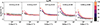Fig. 4. Effective source density estimated from the effective number of source, Eq. (9), and the geometric area of the radial bins stacked in bins of cluster redshift (panels, lowest redshift left, higher redshift right) and of richness (color coding) as stars, for our background selection. Cluster members contaminating our background source sample leads to an increase of the effective source density toward the cluster center, which depends on both cluster richness and redshift. This signal needs to be determined, as cluster member contaminants are not sheared and dilute the shear estimator. Our model (lines) captures this trend well.

We fit the effective number density of cluster members as a function of projected radius R for a cluster of richness λ and redshift z as

$$\begin{array}{c}\hfill n_{\mathrm{eff}}(R|\lambda ,z)=\frac{n_{\mathrm{field}}(z)}{1-f_{\mathrm{cl}}(R|\lambda ,z)},\end{array}$$(14)

where the effective number density in the field n_field(z) is extracted around our clusters in the outer regions, 11 h⁻¹ Mpc < R < 15 h⁻¹ Mpc. This choice of background is designed to measure the excess source lens clustering induced by the photometric misclassification of cluster members as background sources, which is the sole goal of the cluster member contamination correction.

For the fit of the parameters of the cluster member contamination, p_cl= (A_j, B_λ, c), we set up a Gaussian likelihood for the effective number density measured in the above mentioned richness-redshift bins. Our data vector, the effective source density, results from the weighted sum of all tomographic redshift bins (see Eq. (9)). We therefore fit one global cluster member contamination for our overall background selection. We assume a covariance matrix that combines Poisson noise from the effective number of sources and the variance we find in the outer radial bin as a proxy for the cosmic variance in the source density. Sampling this likelihood together with the regularization likelihood gives us constraints on the parameters of the cluster member contamination.

Source redshift distribution decomposition. The estimate from the effective source density around clusters needs to be validated independently, as in the current implementation, we did not consider source obstruction and masking. As demonstrated by Varga et al. (2019), and applied by McClintock et al. (2019), Paulus (2021), Shin et al. (2021), Bocquet et al. (2023), cluster member contamination can also be determined by decomposing the source redshift distribution as a function of the radius into a field component and a Gaussian component of cluster members, that is,

$$\begin{array}{c}\hfill P(z_{\mathrm{s}}|R,\lambda ,z)=(1-f_{\mathrm{cl}}(R|\lambda ,z)){\widehat{P}}_{\mathrm{field}}(z_{\mathrm{s}}|z)+f_{\mathrm{cl}}(R|\lambda ,z)P_{\mathrm{cl}}(z_{\mathrm{s}}|z),\end{array}$$(15)

where the field source redshift distribution ${\widehat{P}}_{\mathrm{field}}(z_{\mathrm{s}}|z)$ is measured in the outer radial bin. The cluster member component is modeled as a Gaussian P_cl(z_s|z) = 𝒩(z_s|z + μ(z),σ²(z)) with mean offset μ(z) = μ₀ + μ_z(z − z₀), and standard deviation σ(z) = σ₀ + σ_z(z − z₀), with pivot z₀ = 0.3, close to the cluster redshift median. This technique adapts the method proposed by Gruen et al. (2014) to wide photometric surveys with readily available photometric redshift estimates. Given that we fit for the shape of a normalized source redshift distribution, the amount of masking does not impact this inference. The likelihood is

$$\begin{array}{c}\hfill ln{\mathcal{L}}_{\beta }=\sum N_{\mathrm{eff}}{\widehat{P}}_{\beta }(z_s)lnP(z_{\mathrm{s}}|R,\lambda ,z)\mathrm{for}\beta \in (bpz,dnf),\end{array}$$(16)

where the sum runs over richness, cluster redshift, cluster-centric distance and source redshift bins². Sampled together with the regularization likelihood, this provides us with constraints on the parameters of the cluster member contamination. We perform this fit for redshift distributions constructed both for BPZ and DNF photo-zs.

Results and comparison. The best-fit results of the number density fit are over-plotted as lines on the effective source density data in Fig. 4, demonstrating that our model can capture the trends in the data well. Furthermore, we find a concentration for the contaminants profile of c = 2.5 ± 0.1. This matches the concentration values found for the galaxy populations of massive clusters (Hennig et al. 2017). Our results also indicate a slight richness slope of the contamination fraction of B_λ = 0.47 ± 0.1. The redshift evolution is shown in Fig. 5 in green (with the filled band corresponding to the 1-sigma uncertainty region and the green lines indicating the 2-sigma). For a cluster at richness pivot λ = 25 at a cluster-centric distance of R = 1 Mpc, we find that the contamination fraction increases from around f_cl ≈ 0.01 at z_cl = 0.1 to f_cl ≈ 0.05 for z_cl > 0.5, with the strongest increase happening between redshifts 0.25 < z < 0.4. We will use this setting to gauge the impact of the different cluster member contamination fits with respect to other systematics.

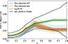Fig. 5. Cluster redshift trend of the cluster member contamination of a richness λ = 25 object at 1 Mpc from the cluster center. In green, the fit to the effective source number density, while in blue and orange, the constraints from the DNF and BPZ source redshift distribution decomposition are shown. The latter method is independent of masking. While we find marginal agreement between the contamination fractions determined by the two methods, the difference is smaller than the relative error induced by shape and photo-z systematics – plotted in black extending from the source density fit for comparison.

As our source selection is discontinuous as a function of lens redshift, we investigate the stability of our results with respect to to the presence of the regularisation condition (Eq. (13)), which might impose an unphysical constraint on the cluster member contamination. As discussed above, we exclude the second tomographic redshift bin for lens redshifts z_l > 0.47. This could induce a sudden reduction of the cluster member contamination. We explore the impact of this by fitting the source redshift decomposition without the regularisation likelihood. We forego a rebinning of our data, as the first four redshift bins up to z_l > 0.48 comprise mainly lenses for which we did not exclude the second tomographic redshift bin. Similarly, most lenses of the highest lens redshift bin, 0.48 < z_l < 0.8, utilize the third and fourth tomographic bins, as we exclude the third tomographic bin for lenses with z_l > 0.74. We find shifts in the amplitude parameter no larger than |ΔA_j|< 0.1, mostly in the last to lens redshift bins. This implies that the regularisation impacts the cluster member contamination f_cl no more than 10% in relative terms, and |Δf_cl|< 0.004 in absolute term. These shifts are negligible compared to other sources of systematic uncertainty, as discussed below.

The source redshift distribution decomposition fits are validated by plotting differences between the measured source redshift distribution and the re-scaled field distribution, as shown in Fig. 6 for 1 Mpc from the center. This subtraction clearly highlights an approximately Gaussian component, that is well described by our model, plotted as full lines. The low amplitude negative dips at source redshifts slightly larger than the Gaussian component show that our field re-scaling, and thus our cluster member estimate, is imperfect. These residuals are clearly smooth in nature, making it very unlikely that they are of statistical origin. They might be systematically due to an alteration of the source redshift distributions in cluster lines of sight. Nonetheless, they are less than 1% in amplitude. This is within our systematic error budget, as discussed below (see Sect. 3.3.2). We therefore accepted the source redshift distribution decomposition as a valid fit.

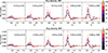Fig. 6. Validation of the source redshift distribution decomposition for DNF (top) and BPZ (bottom) source redshift estimates. In different richness (color coded) and redshift bins (different panels), we show the difference between the source redshift distribution measured along the cluster line of sights and the field distribution extracted at a safe distance from the cluster center, shown as stars. Both are shown here for the projected cluster-centric distance of 1 Mpc in our reference cosmology. The resulting increment is well modeled by a Gaussian component (lines) caused by the cluster members contaminating the source sample. The amplitude of this component scales with cluster richness.

Constraints on the concentration of the contaminants profile and the richness trend of the contamination fraction are in statistical agreement between the fit to the effective number density and the source redshift distributions. The contamination fraction resulting from the source redshift distribution is plotted in Fig. 5. It shows qualitative agreement with the contamination fraction constrained from the effective source density at low redshift. We will argue in the following, why the high redshift differences will not bias the mass calibration.

3.3.2. Shape measurement and photo-z uncertainty

We compare the difference between the cluster member contamination estimates to the shape and photo-z measurement uncertainties of the DES Y3 data as follows. The shape and photo-z uncertainties of the tomographic redshift bin b are summarized by realizations of the source redshift distributions, P_ℋ(z_s|b), running over a hyperparameter ℋ. The variation in the shape of these distributions expresses the uncertainty in the photo-z calibration, while variation in the normalization expresses uncertainties in the multiplicative shear bias 1 + m, as described in more detail in Cordero et al. (2022). Folding this together with our background selection, implemented via lens-redshift dependent weights w_b for the different tomographic redshift bins b (e.g., Eq. (7)), we find a fractional uncertainty of mean lensing efficiency

$$\begin{array}{c}\hfill r_{g_{\mathrm{t}},\mathrm{s}}=\frac{\sqrt{{\mathrm{Var}}_{\mathcal{H}}[\sum _b{w}_b\int \mathrm{d}{z}_{\mathrm{s}}{P}_{\mathcal{H}}(z_{\mathrm{s}}|b){\mathrm{\Sigma }}_{\mathrm{crit},\mathrm{ls}}^{-1}]}}{{\mathrm{E}}_{\mathcal{H}}[{\sum }_b{w}_b\int \mathrm{d}{z}_{\mathrm{s}}{P}_{\mathcal{H}}(z_{\mathrm{s}}|b){\mathrm{\Sigma }}_{\mathrm{crit},\mathrm{ls}}^{-1}]},\end{array}$$(17)

which we take to express the impact of shear and photo-z measurement uncertainties on the measured shear profiles. As the source redshift distributions for the tomographic redshift bins are already response-weighted, no further response-weighting is necessary for the expression above.

The fractional uncertainty increases from 0.55% at z_cl = 0.1 to 4.3% at z_cl = 0.8. We plot these systematic uncertainties around the best-fit values for our cluster member contamination from the effective source density in Fig. 5. The difference between our different cluster member contamination estimates is smaller than this systematic uncertainty. We therefore concluded that we can determine the cluster member contamination to a higher accuracy than provided by the shape and photo-z measurement uncertainties.

3.3.3. Shape noise

In Fig. 7, we show the measured effective shape noise as a function of cluster redshift and richness and as a function of cluster-centric projected distance. The effective shape noise increases with cluster redshift and richness and decreases toward the cluster center. In conjunction with the cluster member contamination estimate from the previous section, we can reconstruct the effective shape noise of cluster members from this decrement. To this end, we fit the measured effective shape noise with a squared sum of field shape noise determined in the outskirt of the clusters and an unknown cluster-member shape noise. The latter is found to be between 18% (for 0.1 < z_cl < 0.19) and 6% (for 0.48 < z_cl < 0.80) lower than the field shape noise, with the trend steadily decreasing with redshift. Given that most of the signal-to-noise in cluster mass measurements comes from scales larger than R > 1 h⁻¹ Mpc, we ignore this effect. In future work, we aim to investigate if this is due to cluster member galaxies being inherently rounder, if the survey-averaged shear response is impacted by the stronger blending in the crowded cluster lines of sight, or if cluster members are just brighter, and therefore have a smaller shape measurement uncertainty contribution to the effective shape noise.

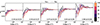Fig. 7. Effective shape noise as a function of cluster-centric distances stacked in bins of cluster redshift (panels: lowest redshift left, higher redshift right) and of richness (color coding). Despite significant scattering, increasing toward the cluster center, a trend of lower-shaped noise toward the center is visible. As gray horizontal lines, the effective shape noise in the field, used for the semi-analytical covariance of the shear profiles, is shown.

For our shape noise modeling, we instead focus on these larger scales, where we measure that the effective shape noise increases with source redshift, as shown in Fig. 8, both for the tangential and the cross component. This trend matches the survey averaged effective shape dispersion found by Friedrich et al. (2021) for the tomographic redshift bins. For later use in our semi-analytical covariance matrix modeling, we fit this trend with the quadratic expression

$$\begin{array}{c}\hfill {\sigma }_{\mathrm{eff}}(z_{\mathrm{cl}})=0.2635+0.0300z_{\mathrm{cl}}^2-0.0008z_{\mathrm{cl}}.\end{array}$$(18)

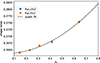Fig. 8. Cluster redshift trend of the effective shape noise in the field (shown as blue and orange diamonds for the cross and tangential reduced shear, respectively). Given our cluster redshift-dependent background selection, the mix of source galaxies changes as a function of cluster redshift. The trend is well-fitted by a quadratic expression, shown as a black dashed line.

This fit is shown as a dashed line in Fig. 8, excellently matching the trend we measure in the data. Extrapolated to z_cl → 0, it matches closely the value reported by Gatti et al. (2021). Without a reliable estimate for the uncertainty of the effective shape noise, we forego reporting error bars on this fit, using it as an effective smoothing to avoid noise on the error estimate of our target quantity, the reduced shear profile.

3.3.4. Cross-shear

Using our fitting formula for the effective shape noise, for each bin in richness and lens-redshift, we can compute the consistency of the cross-shear signal with zero as

$$\begin{array}{c}\hfill {\chi }_{\mathrm{x}}^2=\sum _{\mathrm{r}-\mathrm{bins}}\frac{g_{\mathrm{x}}^2{N}_{\mathrm{eff}}}{{\sigma }_{\mathrm{eff}}^2}·\end{array}$$(19)

These squared losses follow a chi-squared distribution with n_r degrees of freedom, where n_r is the number of radial bins we consider, as shown in Fig. 9. This demonstrates that our cross-shear component averages to zero, consistently with the expectation of well calibrated shape measurements distorted by gravity. We also visually inspect the cross-shear profiles in the above-defined richness and redshift bins and find no significant deviations from zero. Computing instead the global degree of consistency of the raw tangential reduced shear profiles with zero, we find a signal-to-noise of 92³.

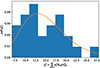Fig. 9. Distribution of the uncertainty-scaled squared residuals of the cross-shear profile with respect to zero signal, as a blue histogram. In orange, the chi-squared distribution for 15 degrees of freedom matches the number of radial bins. The squared loss distribution is well described by the chi-squared distribution, indicating that the cross-shear profiles are consistent with zero given our shape noise modeling.

3.3.5. Shear response

As a further validation test of our WL measurement, we compute the mean shear responses in richness, redshift, and distance bins, given by

$$\begin{array}{c}\hfill \mathcal{R}=\frac{{\sum }_{b=2,3,4}{w}^b{\sum }_{i\in b}{w}_i^{\mathrm{s}}{\mathcal{R}}_i}{{\sum }_{b=2,3,4}{w}^b{\sum }_{i\in b}{w}_i^{\mathrm{s}}}\mathrm{for}\alpha \in (t,x),\end{array}$$(20)

shown in Fig. 10.

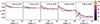Fig. 10. Average shear response, as a function of cluster-centric distance, stacked in bins of cluster richness (color coded), and cluster redshift panels: lowest redshift left, higher redshift right. Noticeably, the shear response increases toward the cluster center. Interestingly, this signal seems to affect all lens redshift bins equally, independently of their cluster member contamination levels. We account for this effect in the cosmology-ready data products.

Notably, the shear response increases toward the cluster center while also showing a gentle trend with richness. The shear response used here is a smooth function of the source relative size with respect to the PSF and its signal-to-noise. Cluster member galaxies are both larger and brighter than the average field population, which could explain the trend we see. However, this signal seems to affect all lens redshift bins equally, independently of their cluster member contamination levels. Another contributing effect could be that field galaxies in cluster lines of sight are magnified by the cluster potential, altering their sizes and signal-to-noise ratios compared to the field galaxies. While interesting, at the scales that we will use for mass calibration, R > 0.5 h⁻¹ Mpc, the effect is smaller than 1%. We can thus safely ignore it in light of the other, larger systematic uncertainties. We plan to investigate how these properties are impacted by cluster lines of sight in future work.

3.4. Selection response

The quantities that we use for our source selection are impacted by the shear we try to measure. For instance, the flux of a sheared galaxy is different from the flux of the original galaxy if it was not sheared. This means that the shear we try to measure impacts our selection of source galaxies and biases our estimators. To correct this bias, we have to measure how our estimator fares on catalogs selected from artificially sheared versions of the actual DES Y3 images. Four such catalogs have been created, each with an artificial shear of Δγ = 0.01 positive/negative (+/–) on the first/second Cartesian component. The selection response in richness, redshift, and distance bins, is given by

$$\begin{array}{cc}\hfill {\mathcal{R}}_{\alpha ,\mathrm{sel}}& =\frac{{\mathcal{R}}_{\alpha ,\mathrm{sel},1}+{\mathcal{R}}_{\alpha ,\mathrm{sel},2}}{2}\hfill \\ \hfill & =\frac{1}{2\mathrm{\Delta }\gamma }({⟨g_{\alpha ,\mathrm{raw}}⟩}^{1+}-{⟨g_{\alpha ,\mathrm{raw}}⟩}^{1-}+{⟨g_{\alpha ,\mathrm{raw}}⟩}^{2+}-{⟨g_{\alpha ,\mathrm{raw}}⟩}^{2-}),\hfill \end{array}$$(21)

for α ∈ (t, x). Here ⟨g_α,  raw⟩¹⁺ denotes the tangential reduced shear estimator on the source sample extracted from the images that have been artificially sheared in positive (+) direction along the first (1) Cartesian shear component, and similarly for the negatively sheared images (−), and the second Cartesian component (2), respectively. The radial, richness, and redshift trends of the selection response are shown in Fig. 11. Especially for high cluster redshift bins, the selection response is very noisy such that no evident trends can be made out.

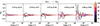Fig. 11. Selection response of our tangential (full lines) and cross (dashed lines) shear estimator, averaged over artificial shears in the two Cartesian coordinates, as a function of cluster-centric distance, stacked in bins of cluster richness (color coded), and cluster redshift panels: lowest redshift left, higher redshift right. The selection response is very noisy but shows no significant trends with richness or cluster-centric distance.

A reliable estimate can thus only be obtained after averaging over richness and radius. We find that the global selection response is positive and bounded by ℛ_α,  sel < 0.001 for z_cl < 0.48, and ℛ_α,  sel ∼ 0.004 for 0.48 < z_cl < 0.8.

Direct comparison between the mean shear responses and the selection response shows that the latter is of order 0.1% of the former for z_l < 0.4, increasing to 0.5% for the redshift bin 0.48 < z_l < 0.8. In both cases, this is a factor of a few less than the uncertainty induced by shape and photo-z measurements and, as such, can be ignored. This assessment contrasts the selection response’s impact on galaxy-galaxy lensing studies (Prat et al. 2022). The main difference is that we do not consider each tomographic bin independently but rather make a selection based on the lens redshift. For low lens redshifts, z_l < 0.48, we thus include a large fraction of the total source sample, reducing the impact of selection effects compared to a tomographic redshift bin selection. At high lens redshift, 0.48 < z_l < 0.8, the close proximity of the source sample to the lens dramatically increases the effects of photo-z uncertainties on the lensing efficiency, dwarfing the effect of the selection response.

Cosmology-ready data products. Given the various distance dependencies of the WL signal, the mass calibration is cosmology-dependent. To marginalize this dependency in this work and to enable the WL mass calibration of our sample self-consistently with the cosmological number counts experiment in Ghirardini et al. (2024), we need to define cosmology-independent data products. Furthermore, given that we pursue a Bayesian population analysis in which each individual cluster likelihood is evaluated, we construct the following data products for each cluster in the cosmology sample that has DES Y3 lensing information:

– the measured reduced shear profile

$$\begin{array}{c}\hfill {\widehat{g}}_{\mathrm{t}}=\frac{{\sum }_{b=2,3,4}{w}^b{\sum }_{i\in b}{w}_i^{\mathrm{s}}{e}_{\mathrm{t},b,i}}{{\sum }_{b=2,3,4}{w}^b{\sum }_{i\in b}{w}_i^{\mathrm{s}}{\mathcal{R}}_i},\end{array}$$(22)

in radial bins with 0.5 h⁻¹ Mpc < R < 3.2(1 + z_cl)⁻¹ h⁻¹ Mpc, in our reference cosmology. The outer bin is chosen following Grandis et al. (2021a) to limit our extraction to the 1-halo term region. We use only the shear response ℛ_i, and ignore the selection response, as argued in Sect. 3.4;

– the statistical uncertainty on the reduced shear,

$$\begin{array}{c}\hfill \delta g_{\mathrm{t}}=\frac{{\sigma }_{\mathrm{eff}}(z_{\mathrm{cl}})}{\sqrt{N_{\mathrm{eff}}}}\mathrm{with}{N}_{\mathrm{eff}}=\frac{{\left({\sum }_{b=2,3,4}{\sum }_{i\in b}{w}^b{w}_i^{\mathrm{s}}{\mathcal{R}}_i\right)}^2}{{\sum }_{b=2,3,4}{\sum }_{i\in b}{\left(w^b{w}_i^{\mathrm{s}}{\mathcal{R}}_i\right)}^2},\end{array}$$(23)

in the same bins. Note here that we use the quadratic fit to the global shape noise given in Eq. (18) to suppress the noise in the individual shear variance estimators;

– the average angular distance of the binned sources from the cluster position in the corresponding radial bins

$$\begin{array}{c}\hfill \theta =\frac{{\sum }_{b=2,3,4}{w}^b{\sum }_{i\in b}{w}_i^{\mathrm{s}}{\mathcal{R}}_i{\theta }_i}{{\sum }_{b=2,3,4}{w}^b{\sum }_{i\in b}{w}_i^{\mathrm{s}}{\mathcal{R}}_i}·\end{array}$$(24)

We report the angular scale, because in the cosmological inference, the distance–redshift relation needs to be self-consistently re-calculated while the data binning is frozen, and

– the field source redshift distribution extracted in the outer regions of the cluster (11 h⁻¹ Mpc < R < 15 h⁻¹ Mpc) based on the SOM-Pz redshift estimation method,

$$\begin{array}{c}\hfill P(z_{\mathrm{s}})=\frac{{\sum }_{b=2,3,4}{w}^b{\sum }_{i\in b}{w}_i^{\mathrm{s}}{\mathcal{R}}_{i}P(z_{\mathrm{s}}|{\widehat{c}}_i)}{{\sum }_{b=2,3,4}{w}^b{\sum }_{i\in b}{w}_i^{\mathrm{s}}{\mathcal{R}}_i},\end{array}$$(25)

where ${\widehat{c}}_i$ is the SOM cell in which the respective source falls. This extraction ensures that our source redshift distribution is a representation of the local field sources.

Using these scale cuts, we reduce the signal-to-noise ratio in the tangential reduced shear to 65. These cuts are necessary to avoid the increased systematic uncertainty toward the cluster centers (see Grandis et al. 2021a, Sect. 3.2). The upper limit was chosen to limit our WL observable to the 1-halo regime for high mass systems, M_500c > 2 × 10¹⁴ h⁻¹ M_⊙. As such, we avoid the 2-halo regime with its more complicated cosmology dependence and possible effects of assembly bias for a majority of our cluster sample and in the higher WL signal-to-noise regime.

4. Calibration of mass extraction

Proper cosmological exploitation of the data products derived above must accurately map the WL signal to the halo mass used in the number counts experiment. In this work, we follow the approach of Grandis et al. (2021a) by simulating synthetic shear profiles starting from hydrodynamical simulations, WL survey specifications, and characteristics of the lens sample. The actual mass measurement is performed on the synthetic shear profiles, resulting in the so-called WL mass, which displays a bias and scatter with respect to the true halo mass. Priors on the WL bias and scatter are derived from Monte Carlo realizations of the synthetic shear profiles, which sample the range of systematic uncertainties on the input specifications. The different simulation inputs used for this calibration are summarized in Table 1.

4.1. Hydrodynamical simulations input

We base the creation of our synthetic shear profiles on the surface mass maps of halos with M_200c > 3 × 10¹³ h⁻¹ M_⊙, extracted with the technique outlined in Grandis et al. (2021a) from the cosmological hydrodynamical TNG300 simulations (Pillepich et al. 2018; Marinacci et al. 2018; Springel et al. 2018; Nelson et al. 2018, 2019; Naiman et al. 2018) at redshifts z_snap = 0.24,  0.42,  0.64,  0.95. To boost the statistical sample size, for each halo, we created three maps by projecting them along each Cartesian coordinate. As described in Grandis et al. (2021a), these maps are processed into scaled tangential shear Γ_t(R,  ϕ|R_mis) and scaled convergence Σ(R,  ϕ|R_mis) maps, binned in polar coordinates (R, ϕ) around isotropically mis-centered positions for a range of mis-centering distances R_mis. Σ(R,  ϕ|R_mis) is the surface mass density in units of h M_⊙ Mpc², which multiplied by the inverse critical surface density gives the convergence, $\kappa ={\mathrm{\Sigma }}_{\mathrm{crit}}^{-1}\mathrm{\Sigma }$. The definition of Γ_t has been introduced in Grandis et al. (2021a) to signify the result of applying the inverse of Kaiser–Squires algorithm to the surface mass density Σ(x), and then determining the tangential component with respect to the chosen center. As both these operations are linear, the resulting quantity is directly related to the tangential shear map as ${\gamma }_t(R,\varphi |R_{\mathrm{mis}})={\mathrm{\Sigma }}_{\mathrm{crit}}^{-1}{\mathrm{\Gamma }}_t(R,\varphi |R_{\mathrm{mis}})$. Being independent from the specific source redshift distribution, this is a convenient simulation output.

This data format conserves the azimuthal anisotropy sourced by the halo triaxiality and by the mis-centering. Possible inaccuracies induced by the correlation between halo shape and mis-centering direction, recently highlighted by Sommer et al. (2023), have been shown to not significantly impact the cosmological results derived from the mass calibration presented in this work (see Ghirardini et al. 2024, Sect. 5.1), but likely need to be accounted for in future analyses with larger statistical constraining power.

Note also that we employ in this work the strategy to mitigate hydrodynamical modeling uncertainties proposed by Grandis et al. (2021a) and used by Chiu et al. (2022, 2023), Bocquet et al. (2023). The hydrodynamical simulations from which we source the surface density maps have gravity-only twin runs with the same initial conditions. It is well established that both runs form exactly the same halos (Castro et al. 2021; Grandis et al. 2021a), albeit with different masses. We purposefully choose the fictitious mass in the gravity-only simulation, as the halo mass functions used in the number counts experiment are calibrated on gravity-only simulations. We can thus use these calibrations to absorb the effects of hydrodynamical feedback on the mass distributions of massive halos in the mapping between the (gravity-only) halo mass and the WL mass, and account for the uncertainty in this mapping in the systematic error budget (see Sect. 4.5).

4.2. Mis-centering

A faithful simulation of synthetic shear profiles requires us to account for the fact that the observed position of the lens is mis-centered from the projected position of the true halo center, which is defined consistently through this work as the position of the most bound particle. The surface mass maps are centered around this position (Grandis et al. 2021a).

We distinguish two sources of mis-centering: (1) the offset between the noise-free peak of the 2d X-ray surface brightness profile and the 2d position of the halo center (hereafter called intrinsic), and (2) the offset between the noise-free peak of the 2d X-ray surface brightness profile and the measured X-ray position (hereafter called observational). The latter displacement is induced by the photon shot noise and the PSF of the eROSITA cameras and is a special case of the astrometric uncertainty discussed in Merloni et al. (2024).

4.2.1. Intrinsic mis-centering

The intrinsic mis-centering is studied through the use of Box2b/hr of the hydrodynamical cosmological simulation suite MAGNETICUM PATHFINDER⁴ (Dolag et al., in prep.), performed assuming the WMAP-7 cosmology as Ω₀ = 0.272 and h = 0.704 as given by Komatsu et al. (2011). The volume of the Box2b/hr box is (909 cMpc)³, allowing for a broad range of galaxy cluster masses up to virial masses M_vir of several times 10¹⁵ M_⊙. The galaxy cluster sample, comprised of 116 clusters with M_vir ≥ 10¹⁴ M_⊙ at z = 0.252, is described in detail in Kimmig et al. (2023). We select an additional 75 galaxy clusters at z = 0.518 to account for redshift trends. The second sample is taken from a different box of equal resolution, Box2/hr of size (500 cMpc)³, to avoid double counting the halos at different redshifts.

Every cluster is projected from 100 random viewing angles. We then determine the projected center-of-mass via the shrinking sphere method (Power et al. 2003) and around this center, the peak of the X-ray emission between 0.5 − 2 keV. The intrinsic mis-centering is then the projected displacement between the X-ray peak and the center of the halo, given by the most-bound particle.

We find that the mis-centering is well described by a single Rayleigh distribution with mean $\langle R_{\mathrm{mis}}^{\mathrm{intr}}\rangle ={\sigma }_{\mathrm{intr}}{R}_{500\mathrm{c}}$, with σ_intr = 0.104 ± 0.016, and with no further resolved mass or redshift trends. As shown below in Sect. 4.5 and Fig. 12, this uncertainty is not relevant when taken together with other systematic effects, especially photometric source redshift and hydrodynamical modeling uncertainties. Valid concerns about the fidelity of the Magneticum prediction of the surface brightness in inner cluster regions are therefore unlikely to impact our results. In future analyses, we plan to validate the centering choice more carefully, for instance, through the blind comparison of the results based on different centers (as done for instance by Bocquet et al. 2023).

Fig. 12. Joint distribution on the WL bias and scatter parameters $(b_l^{\text{WL}},s_l=\ln {({\sigma }_l^{\text{WL}})}^2)$, and their mass slopes ($b_{\mathrm{M}}^{\mathrm{WL}}$, σM), along with the principal sources of systematic uncertainty: the lensing efficiencies Σcrit, l to the snapshots l, in units of 1015 h M⊙ Mpc−2, and the scale of the intrinsic mis-centering σintr. The high redshift biases anticorrelate with the respective lensing efficiencies, indicating that in this regime, we are limited by the DES Y3 photo-z accuracy. Conversely, the low redshift biases and the scatter values correlate among themselves, as they are dominated by the hydro uncertainty floor we added. Insert: Redshift interpolation of the WL lensing bias in cyan (filled region 1 sigma, faded lines 2 sigma), together with the 1 sigma uncertainty due to hydro modeling (green), explorations of the mean impact of the multiplicative shear bias m modeling (red), and the additional omission of the high mis-centering tail f = 0 (dashed red), and the posteriors of the WL bias in the four snap-shots. Hydrodynamical modeling uncertainties are dominant at low redshift. When considering our multiplicative shear bias modeling choices, the bias is consistent with zero, while the presence of the highly mis-centered tail does not affect the WL bias.

4.2.2. Observational mis-centering

For the observational mis-centering, we use the offset θ_sep between input and output positions of clusters in the “eROSITA all-sky survey twin” (Comparat et al. 2019, 2020; Seppi et al. 2022), which produces and analyses simulations of the X-ray signature from a realistic active galactic nucleus and cluster population in eRASS1 observational conditions that include exposure time variations and background. Furthermore, the X-ray cluster finding algorithm, as described in Merloni et al. (2024), Bulbul et al. (2024) is run on the event file generated from this simulation, ensuring that PSF and shot noise of the real observations are well mapped. We select the input clusters matched with simulated sources that have detection likelihood ℒ_det > 3, extent likelihood ℒ_EXT > 6, and extent 4 ≤ EXT ≤ 60, to match the real cosmology sample. For each such object, we compute the separation θ_sep between input and output position, using the entries described in Table A.1 by Seppi et al. (2022).

We model the distribution of mis-centering with a mixture of a Rayleigh distribution and a Gamma distribution with shape parameter 2 as

$$\begin{array}{cc}\hfill P({\theta }_{\mathrm{sep}}|\langle {\theta }_{\mathrm{sep}}\rangle ,f,\lambda )& =\frac{1}{1+f}\frac{{\theta }_{\mathrm{sep}}}{{\langle {\theta }_{\mathrm{sep}}\rangle }^2}exp(-\frac{1}{2}\frac{{\theta }_{\mathrm{sep}}^2}{{\langle {\theta }_{\mathrm{sep}}\rangle }^2})\hfill \\ \hfill & +\frac{f}{1+f}\frac{{\lambda }^2{\theta }_{\mathrm{sep}}}{{\langle {\theta }_{\mathrm{sep}}\rangle }^2}exp(-\frac{\lambda {\theta }_{\mathrm{sep}}}{\langle {\theta }_{\mathrm{sep}}\rangle }),\hfill \end{array}$$(26)

with the mean observational mis-centering given by

$$\begin{array}{c}\hfill \langle {\theta }_{\mathrm{sep}}\rangle =\langle {\theta }_{\mathrm{sep}}|\alpha ,{\sigma }_0,k\rangle ={\left(\frac{{\mathcal{L}}_{\det }}{38.7}\right)}^{-\alpha }\sqrt{{\sigma }_0^2+k^2\mathtt{E}X{T}^2},\end{array}$$(27)

where ℒ_det is the detection likelihood, EXT the extent, as defined by the best-fit detection beta model, and p_mct = (α,  σ₀,  k,  lnf,  lnλ) are free parameters. f is the fraction of mis-centered objects in the heavy-tailed component, α the detection likelihood trend of the mean observational mis-centering, σ₀ the extrapolated mean observational mis-centering for a point source (EXT = 0), k the slope of the mean mis-centering with respect to the sources extent, and λ the length of the mis-centering tail in units of the mean mis-centering.

We fit these by sampling the likelihood

$$\begin{array}{c}\hfill ln\mathcal{L}=\sum _{v}lnP({\theta }_{\mathrm{sep}}^v|\langle {\theta }_{\mathrm{sep}}^v|\alpha ,{\sigma }_0,k\rangle ,lnf,ln\lambda ),\end{array}$$(28)

assuming flat priors on all parameters, with v running over the clusters selected from the digital twin simulation. All parameters are well constrained; Table 2 reports their means and standard deviations. Noticeably, the mean dependence on the detection likelihood α = 0.43 ± 0.02 is quite close to the α = 0.5 trend one would expect for matched filter extraction in the presence of Gaussian noise (Story et al. 2011; Song et al. 2012). Our constraint on lnf translates into a relative weight of 0.318 ± 0.043 for the flatter Gamma distribution component, albeit only a part of that distribution populates the high mis-centering tail. Our other fit parameters result in a typical mis-centering ⟨θ_sep⟩ ∼ 11 arcsec.

We also check that once the individual mis-centerings are corrected for the typical mis-centering of sources of that detection significance and extent, the residuals show no correlation with exposure time. This ensures that our parametrization captures the main trends of the observational mis-centering and that it can be safely used despite the exposure time varying over the survey footprint. To further validate our model, we draw mock catalogs by selecting a random posterior point p_mct = (α,  σ₀,  k,  lnf,  lnλ). For each simulated cluster, we then compute the typical mis-centering ⟨θ_sep⟩ and draw a mock separation angle θ_sep from Eq. (26). This procedure creates 1000 mock cluster samples that follow our model by drawing 1000 independent posterior points. In Fig. 13 we plot in blue the mis-centering distribution of the actual data, while in orange data points, the distribution of mock data, sampled from our posterior, are shown. The two are indistinguishable, indicating that the actual mis-centering distribution from the digital twin looks like data drawn from our mis-centering model. Comparisons of the maximum likelihood of the data and the mocks show that this also holds at the likelihood level (see insert of Fig. 13). Our observational mis-centering model is therefore a good fit.

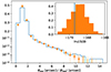Fig. 13. Observational mis-centering between the input X-ray surface brightness peaks and the output positions of clusters in the eROSITA digital twin, θsep, scaled by the best-fit average offset, ⟨θsep⟩, shown in blue as a histogram. Overlaid in orange are realizations of mock offsets drawn from the posterior of our model. The data is indistinguishable from the mock draws. Our model is also validated by comparing, in the insert, the likelihood of the data in blue with the likelihood of the mocks in orange.

4.3. Extraction model

When performing the mass measurement, we need to specify a mass extraction model and coherently apply it to both the real and the synthetic data. In this analysis, we choose a simplified mis-centered model, corrected for the mean cluster member contamination, as suggested by Grandis et al. (2021a). This model faithfully captures the main biases induced by mis-centering and cluster member contamination while not adding numerical complexity compared to the plain 2d-projected NFW model. This approach is well suited for the repeated calls in the Monte Carlo Markov chains used for parameter inference. Bocquet et al. (2023) make the same choices for the same reasons.

For the model, we assume that a cluster of radius R_500c and mean observational mis-centering ⟨θ_sep⟩ is effectively mis-centered by a physical distance

$$\begin{array}{c}\hfill R_{\mathrm{mis}}^{\mathrm{extr}}=\sqrt{({\sigma }_{\mathrm{intr}}{R}_{500\mathrm{c}}{)}^2+{\left(D_{\mathrm{l}}\langle {\theta }_{\mathrm{sep}}\rangle \right)}^2},\end{array}$$(29)

evaluated at the mean of the observational mis-centering parameters determined in Sect. 4.2.2. The radius R_500c is derived from the input mass of the extraction model. The cluster surface mass distribution is then well approximated by

$$\begin{array}{c}\hfill \mathrm{\Sigma }(R|M)=\{\begin{array}{cc}{\mathrm{\Sigma }}_{\mathrm{NFW}}(R_{\mathrm{mis}}^{\mathrm{extr}}|M)\hfill & \mathrm{for}R<R_{\mathrm{mis}}^{\mathrm{extr}},\mathrm{and}\hfill \\ {\mathrm{\Sigma }}_{\mathrm{NFW}}(R|M)\hfill & \mathrm{otherwise},\hfill \end{array}\end{array}$$(30)

where Σ_NFW(R|M) is the 2d projected NFW profile, evaluated with the mean concentration mass relation reported by Ragagnin et al. (2021). Deviations of this concentration mass relation from the one in the simulations are absorbed in the WL bias, while scatter in concentration at fixed mass contributes to the WL scatter. As shown in Bocquet et al. (2023), this surface mass profile results in a radial density contrast ΔΣ(R|M) = 0 for $R<R_{\mathrm{mis}}^{\mathrm{extr}}$, and

$$\begin{array}{c}\hfill \mathrm{\Delta }\mathrm{\Sigma }(R|M)=\mathrm{\Delta }{\mathrm{\Sigma }}_{\mathrm{NFW}}(R|M)-{\left(\frac{R_{\mathrm{mis}}^{\mathrm{extr}}}{R}\right)}^2\mathrm{\Delta }{\mathrm{\Sigma }}_{\mathrm{NFW}}(R_{\mathrm{mis}}^{\mathrm{extr}}|M),\end{array}$$(31)

at a larger projected radius. This expression is numerical of the same complexity as evaluating the 2d density contrast of NFW profile ΔΣ_NFW(R|M) but is significantly more accurate.

We then considered the average lensing efficiency

$$\begin{array}{c}\hfill {\mathrm{\Sigma }}_{\mathrm{crit},\mathrm{l}}^{-1}={\langle {\mathrm{\Sigma }}_{\mathrm{crit},\mathrm{ls}}^{-1}\rangle }_{P_{\mathrm{l}}(z_{\mathrm{s}})}\end{array}$$(32)

of the lens l, obtained by averaging the lensing efficiency of the individual source, ${\mathrm{\Sigma }}_{\mathrm{crit},\mathrm{ls}}^{-1}$, Eq. (3), with the source redshift distribution P_l(z_s). Using also the cluster member contamination fraction f_cl(R|λ, z), evaluated at the mean cluster member contamination parameters, for the cluster richness λ and the cluster redshift z_cl, we defined the reduced shear model:

$$\begin{array}{c}\hfill g_{\mathrm{t}}^{\mathrm{mod}}(R|M)=\frac{{\mathrm{\Sigma }}_{\mathrm{crit},\mathrm{l}}^{-1}\mathrm{\Delta }\mathrm{\Sigma }(R|M)}{1-{\mathrm{\Sigma }}_{\mathrm{crit},\mathrm{l}}^{-1}\mathrm{\Sigma }(R|M)}(1-f_{\mathrm{cl}}(R|\lambda ,z_{\mathrm{cl}})).\end{array}$$(33)

This extraction model also depends on the clusters detection likelihood ℒ_det and extent EXT, and the mean parameters of the mis-centering through the mean extraction mis-centering, Eq. (29). All these quantities are readily available for each cluster.

Any mismatches between the real profiles and the extraction model are captured by considering that the best-fit mass assuming this model, the WL mass M_WL, will be biased and scattered around the true halo mass.

4.4. Synthetic shear profiles

The creation of the synthetic shear profiles proceeds as follows.

1. The redshift of the synthetic clusters is fixed to the redshift of the hydro-simulation outputs.

2. Assuming the mean concentration c_200c–mass relation by Child et al. (2018), we convert the masses M_200c from the simulation to M_500c, using the customary transformations (see for instance Ettori et al. 2011, Appendix A). Note that the concentration–mass relation employed here was calibrated on gravity-only simulations, which matches the fact that our halo masses are also gravity-only masses.

3. We assign a synthetic source redshift distribution $P_l^{\text{snth}}(z_{\text{s}})$ based on the tomographic bin weights w_b(z_l), as defined in Eq. (7), and the realisations of their redshift distribution P_ℋ(z_s|b), as provided by Myles et al. (2021), discussed in Sect. 3.3.2, and shown in Fig. 2. The normalization of these distributions takes account of the multiplicative shear bias.

4. Each cluster is assigned a richness λ based on the richness–mass relation calibrated in Chiu et al. (2022). For later use, we remind the reader that this relation is defined by the parameters of the richness–mass relation p_λM. The richness is required both as an input for the extraction model, as well as to simulate the cluster member contamination, f_cl(R|λ, z_cl, p_cl), on the synthetic shear profile, where p_cl are the parameters of the cluster member contamination.

5. Querying the halos with |Δlog₁₀M_500c/M_⊙|< 0.1 and |Δz|< 0.05 from the eROSITA digital twin, we select the detection likelihood ℒ_det and extent EXT of a random pick. These two observables are needed to define the mean mis-centering needed by the extraction model and to assign a correct mis-centering distribution P(R_mis|M_500c, z, ℒ_det, EXT, p_mct), resulting from the convolution of the observational and intrinsic mis-centering discussed in Sect. 4.2. Note that this step depends on the parameters of the mis-centering p_mct, determined in the same section.

6. Improving on previous work, we now compute the reduced shear not only for each polar position in the map but also for each source redshift z_s, as presented also in Bocquet et al. (2023). The azimuthal and source redshift average are computed after the computation of the reduced shear as follows

$$\begin{array}{c}\hfill g_{\mathrm{t}}^{\mathrm{snth}}(R|R_{\mathrm{mis}})=\int \mathrm{d}{z}_{\mathrm{s}}{P}^{\mathrm{snth}}(z_{\mathrm{s}})\int \frac{\mathrm{d}\varphi }{2\pi }\frac{{\mathrm{\Sigma }}_{\mathrm{crit},\mathrm{ls}}^{-1}{\mathrm{\Gamma }}_t(R,\varphi |R_{\mathrm{mis}})}{1-{\mathrm{\Sigma }}_{\mathrm{crit},\mathrm{ls}}^{-1}\mathrm{\Sigma }(R,\varphi |R_{\mathrm{mis}})}·\end{array}$$(34)

Deviating from this integration order leads to biases in the synthetic profiles of the order of 0.01, which is unacceptable given our accuracy requirements.

7. We add cluster member contamination following the fit we derived in Sect. 3.3.1, specifically the number density fit. We also add a nonlinear shear bias and extra noise from the uncorrelated large-scale structure along the line of sight, as discussed in Grandis et al. (2021a).

8. The extraction of the WL mass via the extraction model and the fit for the WL bias and scatter weighted by the mis-centering distribution follow exactly the method outlined in Grandis et al. (2021a).

The output data product of such synthetic shear profile production and subsequent fit with the extraction model is shown in Fig. 14. There, we plot the input halo masses versus the WL masses, color coded by the mis-centering distribution probability for the respective synthetic halo. Note that extreme outliers in WL mass are associated predominantly with highly mis-centered synthetic clusters and are thus quite rare, given the mis-centering distribution. As such, they contribute only marginally to the fit.

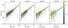Fig. 14. Scatter plot of the input halo mass versus the output WL mass from one realization of the synthetic shear profiles. Color coded by the value of the mis-centering distribution for that specific halos’ mis-centering, and as solid black lines, the mis-centering-distribution-weighted scaling between WL and halo mass, which results in an estimate for the WL bias. The scatter around this relation results in the WL scatter. Generally speaking, extreme outliers also have highly improbable mis-centering.

4.5. WL bias and scatter

At the end of the synthetic shear profile production and WL extraction, we get a bias and scatter $(b_l^{\text{WL}},{\sigma }_l^{\text{WL}})$ for each snapshot l, as well as a mass trend for both the bias ($b_{\mathrm{M}}^{\mathrm{WL}}$), and the scatter (s_M). They were obtained by fitting the relation

$$\begin{array}{cc}\hfill \langle ln\frac{M_{\mathrm{WL}}}{M_0}|M,z_{\mathrm{cl}}\rangle & =b_l^{\mathrm{WL}}+b_{\mathrm{M}}^{\mathrm{WL}}ln\left(\frac{M}{M_0}\right)\hfill \\ \hfill ln{\sigma }_{\mathrm{WL}}^2& =s_l+s_{\mathrm{M}}ln\left(\frac{M}{M_0}\right),\hfill \end{array}$$(35)

with pivot mass M₀ = 2 × 10¹⁴ M_⊙, and $s_l=\ln {({\sigma }_l^{\text{WL}})}^2$. The fit of the relation includes cluster-by-cluster weights corresponding to the probability of the mis-centering of the individual synthetic halo, as discussed in Grandis et al. (2021a). The mean relations resulting from the fit at each redshift are shown in Fig. 14 as black lines.

Systematic uncertainty estimation. The uncertainty on these quantities is obtained by re-running the synthetic shear profile creation and WL mass extraction 𝒪(1000) times with slightly perturbed input parameters. Specifically, we vary the hyperparameter of the DES Y3 source redshift distributions ℋ ∈ (0, 999) (Myles et al. 2021, and as outlined in Sect. 3.3.2), the parameters of the richness–mass relation p_λM within the posterior reported by Chiu et al. (2022), the parameters of the cluster member contamination p_cl within the posterior determine in Sect. 3.3.1, the parameters of the mis-centering distribution p_mct within the posterior determine in Sect. 4.2, as well as a wide prior on the nonlinear shear biases. To these uncertainties, we add a hydrodynamical modeling uncertainty of 2% on the WL bias and corresponding values for the other parameters, as determined by Grandis et al. (2021a, Table 2).

The resulting parameter posterior distributions are presented in the contour plots in Fig. 12. We omit parameters that do not (anti)correlate with the WL bias and scatter parameters. These include, but are not limited to, the parameters of the richness mass relation p_λM. This indicates that the weak lensing bias calibration is insensitive to the richness assignment in our synthetic simulations. Indeed, the extraction model (Eq. (33)) and the synthetic shear profiles depend in very similar ways on the richness via the cluster member contamination. To first order the assumed richness–mass relation thus cancels. Also, the nonlinear multiplicative shear bias α_NL does not affect our systematics despite its large uncertainty. Despite the stronger shears expected in cluster lines of sight compared to the field, we thus do not require a dedicated nonlinear shear bias calibration.

We also report critical surface densities ${\mathrm{\Sigma }}_{\mathrm{crit},l}={\langle {\mathrm{\Sigma }}_{\mathrm{crit},s,l}^{-1}\rangle }_{P_l^{\mathrm{snth}}(z_{\mathrm{s}})}^{-1}$ for each snapshot l, defined as the inverse lensing efficiency, reported in units of 10¹⁵ h M_⊙ Mpc⁻². This helps visualize the impact of the marginalization over the photometric redshift uncertainties, which is implemented via the hyperparameter ℋ. As can be seen in Fig. 12, the WL bias in the highest redshift snapshot $b_4^{\text{WL}}$ anticorrelates tightly with the critical surface density ${\mathrm{\Sigma }}_{\mathrm{crit},4}={\langle {\mathrm{\Sigma }}_{\mathrm{crit},s,l=z_4}^{-1}\rangle }_{P_{z_4}^{\mathrm{snth}}(z_{\mathrm{s}})}^{-1}$ This indicates that the uncertainty on this bias parameter is dominated by the uncertainty on the lensing efficiency, as induced by the photo-z uncertainty. The other WL bias parameters have a more gentle correlation with the lensing efficiencies, indicating a smaller impact of photo-z uncertainties in lower redshift clusters.

Compression. In principle, the full distribution of weak lensing biases $b_l^{\text{WL}}$, the logarithm weak lensing squared scatters s_l, as well as their mass trends, should be used as priors for a mass calibration analysis of the actual data to account for the systematic uncertainties. This would, however, significantly bloat the parameter space of that likelihood analysis. As we sample the mass calibration likelihood presented in this work simultaneously with the cosmological inference from number counts in Ghirardini et al. (2024), reducing the number of parameters is of great benefit.

We compress the 4-dimensional posterior on the WL bias parameters $b_l^{\text{WL}}$ into mean values μ_b, l, and two principal components δ_b1, l and δ_b2, l, scaled by their variances. The other two principal components of the 4-dimensional random variable are found to not contribute significantly to the overall scatter in the WL bias posterior. This means that a realization of the WL bias at an arbitrary redshift z_cl can be constructed by interpolating the mean and principal components and drawing two random standard normal variates A_WL, B_WL, such that

$$\begin{array}{c}\hfill b(z_{\mathrm{cl}})=\mathcal{I}(z_{\mathrm{cl}}|z_l,{\mu }_{\mathrm{b},l})+A_{\mathrm{WL}}\mathcal{I}(z_{\mathrm{cl}}|z_l,{\delta }_{\mathrm{b}1,l})+B_{\mathrm{WL}}\mathcal{I}(z_{\mathrm{cl}}|z_l,{\delta }_{\mathrm{b}2,l}),\end{array}$$(36)

where ℐ(z_cl|z_l,  μ_b, l) is the interpolation of the data vectors (z_l,  μ_b, l) at redshift z_cl. The resulting posterior on the WL bias as a function of cluster redshift is shown in the insert of Fig. 12 in blue bands for the 1σ region, and faded lines for the 2σ regions, together with the results for the 4 snapshots as black data points. For the 4 values of the natural logarithm of the variance, whose posterior is dominated by the uncertainty from hydrodynamical modeling, we employ a single principal component (see below, Eq. (45)). We do not compress the mass trends of the bias and the variance. These compressions reduced the number of free parameters from 10 to 5 while still capturing the relevant systematic uncertainties. As we consider 2 principal components for the weak lensing bias, we also represent the systematic uncertainty on its redshift evolution.

Sensitivity study. The numerical value of our WL bias is somewhat low, ranging from −0.05 to −0.1. A contributing factor is the response of the WL bias to our treatment of the multiplicative shear bias. While we include the multiplicative shear bias in the synthetic shear profiles, we do not include this bias in the model to reduce the number of independent calibration products we need to communicate to the cosmological number counts analysis (Ghirardini et al. 2024). To gauge the impact of this modeling choice on the numerical value of the bias, we perform a synthetic shear and mass extraction run at the mean values of all parameters but artificially set the multiplicative shear bias m = 0, that is, we normalize the synthetic source redshift distributions to 1. This results in a shift, shown as the red line in the insert of Fig. 12 of the order of −0.03. It is two sigma away from our inferred bias values (black data points). Discounting for this effect, we would find bias values ranging from −0.03 to −0.07, and thus consistent with zero bias at less than 2σ of our systematic error budget. This qualitatively indicates that our simplified extraction model is a good representation of the much more complex synthetic data. Slightly negative WL biases can be explained by the fact that the density contrast of a halo is reduced by the projection of nearby correlated structure, resulting in a WL mass that is lower than the halo mass (Oguri & Hamana 2011; Becker & Kravtsov 2011; Bahé et al. 2012).

We also test the sensitivity of the WL bias to the presence of the highly mis-centered tail in the eROSITA digital twin (cf. Sect. 4.2). A similar large mis-centering tail is found by Bulbul et al. (2024), Sect. 5 and Fig. 9, left panel, when comparing the centers obtained from the source detection algorithm and the X-ray post-processing. While the origin of this tail is still under investigation, we explore the hypothesis that the large mis-centering tail is completely suppressed by the X-ray post-processing. Setting the fraction f = 0 fully suppresses the high exponential tail but only mildly alters the WL bias, as can be seen by the difference between the red solid and dashed line. Our WL bias numbers, and therefore the mass anchoring of the number counts experiments, are stable with respect to the presence of this highly mis-centered tail, which might be an artifact of the eROSITA digital twin processing, and be corrected by the X-ray post-processing.

Summary. The two main contributions to the uncertainty of the WL bias are the systematic floor resulting from the comparison of different hydrodynamical simulations established by Grandis et al. (2021a), and, at high redshift z_l > 0.6 also the uncertainty of the DES Y3 photometric redshift distributions, shown in Fig. 2. Several other effects we studied, such as mis-centering and nonlinear multiplicative shear bias, do not contribute significantly to the systematic uncertainty of the mass extraction from our WL data. We compress the results of our synthetic simulations via principle component analysis, finding that 5 nuisance parameters are sufficient to represent all the systematic uncertainty trends our simulations revealed.

5. Mass constraints

WL measurements around galaxy clusters provide a highly accurate (see Sect. 4) mass proxy. They have, however, a quite low precision at the individual object basis, considering that the approximately 2.2 k clusters we consider collectively only reach a signal-to-noise of 65 (cf. Sect. 3.4). A natural approach to counter-act this is to perform the mass measurement on stacked lensing signals (e.g. McClintock et al. 2019; Bellagamba et al. 2019). While this simplifies the mass measurement task, it significantly complicates the modeling in a cosmological context by introducing scale-dependent selection bias effects (Sunayama et al. 2020; Dark Energy Survey Collaboration 2020; Wu et al. 2022; Sunayama 2023). In this work, we therefore followed the Bayesian Population modeling approach pioneered by Mantz et al. (2015), Bocquet et al. (2019), Grandis et al. (2019), which predicts the distribution of expected shear profiles given the selection observable as a function of the parameters governing the scaling between halo mass and selection observables. Complete derivations of this analysis framework can be found in Ghirardini et al. (2024), Bocquet et al. (2023) in the context of eROSITA–selected clusters and SPT–selected clusters, respectively. Our results here are based on the implementation described in Ghirardini et al. (2024), Sect. 4.

5.1. Constraints of the count rate–mass relation

In the following, we discuss the likelihood setup used for the mass calibration as well as the resulting mass calibration constraints. In general, WL mass calibration relies on statistically determining the scaling relation between the observables and halo mass (Mantz et al. 2016; Dietrich et al. 2019; Schrabback et al. 2021; Zohren et al. 2022, for instance). In our case, we expand this standard treatment to accommodate for the residual contamination of our sample by random superpositions of X-ray candidates and optical systems and, more importantly, misclassified active galactic nuclei (see Bulbul et al. 2024; Kluge et al. 2024; Ghirardini et al. 2024). Misclassified AGNs and random superpositions are expected to produce far less WL signal than clusters, which inhabit massive halos. We therefore employ a mixture model, a weighted sum of the different sub-populations, to perform the mass calibration in the presence of non-negligible contamination.

5.1.1. Mixture model

For each individual cluster, we construct the probability density function (PDF) of its shear profile g_t given the cluster observables count rate ${\widehat{C}}_{\mathrm{R}}$, redshift z_cl and sky position $\widehat{\mathcal{H}}$ as

$$\begin{array}{cc}\hfill P({\widehat{g}}_{\mathrm{t}}|{\widehat{C}}_R,z_{\mathrm{cl}},\widehat{\mathcal{H}})& =f_{\mathrm{C}}({\widehat{C}}_R,z_{\mathrm{cl}},\widehat{\mathcal{H}})P({\widehat{g}}_{\mathrm{t}}|{\widehat{C}}_R,z_{\mathrm{cl}},\widehat{\mathcal{H}},C)\hfill \\ \hfill & +f_{\mathrm{RS}}({\widehat{C}}_R,z_{\mathrm{cl}},\widehat{\mathcal{H}})P({\widehat{g}}_{\mathrm{t}}|\mathrm{RS})\hfill \\ \hfill & +f_{\mathrm{AGN}}({\widehat{C}}_R,z_{\mathrm{cl}},\widehat{\mathcal{H}})P({\widehat{g}}_{\mathrm{t}}|\mathrm{AGN},z_{\mathrm{cl}}),\hfill \end{array}$$(37)

a weighted sum of the PDF of the shear profile for clusters (C), random superpositions (RS), and misclassified active galactic nuclei (AGN), with their respective frequencies $f_{\tau }({\widehat{C}}_R,z_{\mathrm{cl}},\widehat{\mathcal{H}})$ as a function of count rate, redshift and sky position, where τ∈ (C, RS, AGN). Naturally, $\sum _{\tau }{f}_{\tau }({\widehat{C}}_R,z_{\mathrm{cl}},\widehat{\mathcal{H}})=1$, where the sum runs over τ∈ (C, RS, AGN). As outlined in Bulbul et al. (2024), Kluge et al. (2024), Ghirardini et al. (2024), the shape of the AGN and the random superpositions contributions are calibrated partially on X-ray image simulations, partially with optical follow-up of random positions and point sources, and have amplitudes (f_RS, f_AGN) that are fitted for using the richness distribution of the sample at a given count rate, redshift, and sky position. They find f_RS = 0.0061 ± 0.0023 and f_AGN = 0.0462 ± 0.0038, which we adopt as priors.

For the WL modeling, we assumed that the density contrast of a random source is zero, resulting in their shear profile PDF being

$$\begin{array}{c}\hfill lnP({\widehat{g}}_{\mathrm{t}}|\mathrm{RS})=-\frac{1}{2}\sum _k\frac{{\widehat{g}}_{\mathrm{t},k}^2}{\delta g_{\mathrm{t},k}^2},\end{array}$$(38)

where the sum runs over the radial bins k, with the measured shear profile ${\widehat{g}}_{\mathrm{t},k}$ defined in Eq. (22), and its shape noise error δg_t, k defined in Eq. (23). In practice, all objects in our lens sample have a richness $\widehat{\lambda }>3$. At the lens redshift, the random source will thus have a few red galaxies along their lines of sight. Their density contrast is, however, expected to be small compared to cluster density contrasts.

For AGNs we assume that their density contrast ΔΣ_AGN(R) follows the profile measured by Comparat et al. (2023) for AGN in eFEDS using HSC WL data. We multiply this with the average lensing efficiency ${\mathrm{\Sigma }}_{\mathrm{crit},\mathrm{c}}^{-1}={⟨{\mathrm{\Sigma }}_{\mathrm{crit},\mathrm{cs}}^{-1}⟩}_{P_{\mathrm{c}}(z_{\mathrm{s}})}$, evaluated as a function of cosmology for the source redshift distribution P_c(z_s) constructed in Eq. (25). The PDF thus reads

$$\begin{array}{c}\hfill lnP({\widehat{g}}_{\mathrm{t}}|\mathrm{AGN},z_{\mathrm{cl}})=-\frac{1}{2}\sum _k\frac{1}{\delta g_{\mathrm{t},k}^2}{({\widehat{g}}_{\mathrm{t},k}-{\mathrm{\Sigma }}_{\mathrm{crit},\mathrm{c}}^{-1}\mathrm{\Delta }{\mathrm{\Sigma }}_{\mathrm{AGN}}(R=D_c{\theta }_k))}^2,\end{array}$$(39)

where D_c is the angular diameter distance to the cluster, and θ_k the average angular distance to the sources in the respective radial bin k, as computed in Eq. (24). In practice, the density contrast of AGN is much smaller than that of galaxy clusters, given the lower host halo mass.

For galaxy clusters, the PDF of the shear profile depends on our extraction model $g_{\mathrm{t}}^{\mathrm{mod}}$, and the WL mass M_WL defined by this model (cf. Sect. 4.3). It therefore reads

$$\begin{array}{c}\hfill lnP({\widehat{g}}_{\mathrm{t}}|\mathrm{C},z_{\mathrm{cl}},M_{\mathrm{WL}})=-\frac{1}{2}\sum _k\frac{1}{\delta g_{\mathrm{t},k}^2}{({\widehat{g}}_{\mathrm{t},k}-g_{\mathrm{t}}^{\mathrm{mod}}(R=D_c{\theta }_k|M_{\mathrm{WL}}))}^2,\end{array}$$(40)

with the extraction model depending on a host of cluster-specific observables, as outlined above. Note that in all three PDFs, we omitted the normalization term, which is the same for all three, and just depends on δg_t, k, thus being constant with respect to the parameters of the inference.

The PDF of the shear profile for clusters needs to be marginalized over the distribution of WL masses M_WL compatible with the clusters count rate ${\widehat{C}}_{\mathrm{R}}$, redshift z_cl, and sky position $\widehat{\mathcal{H}}$, that is $P(M_{\mathrm{WL}}|{\widehat{C}}_R,z_{\mathrm{cl}},\widehat{\mathcal{H}},{\mathit{p}}_{\mathrm{SR}})$, whose construction and dependence on model parameters p_SR we shall discuss below. The PDF of the shear profile for the cluster component is thus

$$\begin{array}{cc}\hfill P({\widehat{g}}_{\mathrm{t}}|{\widehat{C}}_R,z_{\mathrm{cl}},\widehat{\mathcal{H}},\mathrm{C})=\int \mathrm{d}{M}_{\mathrm{WL}}& P({\widehat{g}}_{\mathrm{t}}|\mathrm{C},z_{\mathrm{cl}},M_{\mathrm{WL}})\hfill \\ \hfill & P(M_{\mathrm{WL}}|{\widehat{C}}_R,z_{\mathrm{cl}},\widehat{\mathcal{H}},{\mathit{p}}_{\mathrm{SR}}).\hfill \end{array}$$(41)

The distribution of WL masses given the count rate, redshift and sky position is proportional to

$$\begin{array}{cc}\hfill P(M_{\mathrm{WL}}|{\widehat{C}}_R,z_{\mathrm{cl}},\widehat{\mathcal{H}},{\mathit{p}}_{\mathrm{SR}})\propto & \int \int \mathrm{d}M\mathrm{d}{C}_{R}P(M_{\mathrm{WL}},C_R|M,z_{\mathrm{cl}},{\mathit{p}}_{\mathrm{SR}})\hfill \\ \hfill & P(I|C_R,z_{\mathrm{cl}},{\widehat{\mathcal{H}}}_i)P({\widehat{C}}_R|C_R)P(M,z_{\mathrm{cl}}),\hfill \end{array}$$(42)

with $P({\widehat{C}}_R|C_R)$ modeling the observational uncertainty on the count rate, P(M, z_cl) being proportional to the halo mass function, and $P(I|C_R,z_{\mathrm{cl}},{\widehat{\mathcal{H}}}_i)$ the X-ray incompleteness due to the extent selection. This ensures that we correctly model Eddington bias, which manifests as more low-mass objects scattering up to a given observable value than high-mass objects scattering down to the same observable values. This happens even when the observable–mass scatter is modeled as symmetric because there are just many more low-mass than high-mass objects. This fact is quantitatively expressed by the halo mass function. The expression given above is normalized to be a PDF in M_WL via integration in M_WL and subsequent re-scaling. See Ghirardini et al. (2024) for an alternative, but equivalent, derivation of the same likelihood.

5.1.2. Scaling relation

Given their deep potential wells, cluster observables scale tightly with the host halos mass. Leveraging this strong physical prior, we model the distribution of WL mass M_WL and intrinsic (that is noise-free) count rate C_R at given halo mass M and redshift z as a bi-variate log-normal, reading

$$\begin{array}{c}\hfill P(M_{\mathrm{WL}},C_R|M,z_{\mathrm{cl}},{\mathit{p}}_{\mathrm{SR}})=\mathcal{N}(\overline{\mu },\overline{\mathrm{\Sigma }}),\end{array}$$(43)

with mean and variance

$$\overline{\mu }=[\langle ln{C}_R|M,z_{\mathrm{cl}}\rangle ,\langle ln{M}_{\mathrm{WL}}|M,z_{\mathrm{cl}}\rangle ]$$

$$\overline{\mathrm{\Sigma }}=\left[\begin{array}{cc}{\sigma }_{\mathrm{X}}^2& {\rho }_{\mathrm{WL},\mathrm{X}}{\sigma }_{\mathrm{X}}{\sigma }_{\mathrm{WL}}\\ {\rho }_{\mathrm{WL},\mathrm{X}}{\sigma }_{\mathrm{X}}{\sigma }_{\mathrm{WL}}& {\sigma }_{\mathrm{WL}}^2\end{array}\right]$$

where ⟨lnC_R|M,z_cl⟩ and ⟨lnM_WL|M,z_cl⟩ are the scaling relations between true mass and count rate and WL mass, respectively, σ_X and σ_WL their intrinsic scatters, and ρ_WL, X the correlation coefficient between the two intrinsic scatters. Inclusion of the latter is crucial to marginalize over possible selection effects like more concentrated halos simultaneously having a higher count rate and WL mass compared to other objects at their mass and redshift, or any other effect that might similarly correlate the intrinsic scatters.

As calibrated on dedicated simulations in Sect. 4, the mean WL mass – halo mass relation is given by

$$\begin{array}{c}\hfill \langle ln\frac{M_{\mathrm{WL}}}{M_{\mathrm{p}}}|M,z_{\mathrm{cl}}\rangle =b(z_{\mathrm{cl}})+b_{\mathrm{M}}ln\left(\frac{M}{M_{\mathrm{p}}}\right),\end{array}$$(44)

with the pivot value for the mass M_p = 2 × 10¹⁴ M_⊙, the redshift dependent amplitude of the WL bias given by Eq. (36), and the mass trend b_M = μ_bM + C_WL ⋅ σ_bM, with mean and standard deviation derived in Sect. 4.5 and reported in Table 3.

The scatter is similarly modeled as

$$\begin{array}{c}\hfill {\sigma }_{\mathrm{WL}}^2=exp\{\mathcal{I}(z_{\mathrm{cl}}|z_l,{\mu }_{\mathrm{s},l})+D_{\mathrm{WL}}\mathcal{I}(z_{\mathrm{cl}}|z_l,{\delta }_{\mathrm{s},l})\},\end{array}$$(45)

where μ_s, l and δ_s, l are the mean and standard deviations of the WL scatter in the simulation snapshot l, derived in Sect. 4.5 and reported in Table 3, and ℐ(z_cl|z_l,  μ_s, l) is the interpolation of the data vectors (z_l,  μ_s, l) to the redshift z_cl. Given the tight correlations between the systematic uncertainties in the WL scatters of the different redshift seen in Fig. 12, we opt to model the WL scatter with a single principal component. We also set the mass trend of the scatter to s_M = 0 as in this work, we are not interested in exploring mass trends in the intrinsic scatter of the other observables.

The count rate–mass relation is modeled as

$$\begin{array}{c}\hfill \langle ln\frac{C_R}{C_{R,\mathrm{p}}}|M,z_{\mathrm{cl}}\rangle =ln{A}_{\mathrm{X}}+b_{\mathrm{X}}(M,z_{\mathrm{cl}})·ln\frac{M}{M_{\mathrm{p}}}+e_{\mathrm{X}}(z_{\mathrm{cl}})\end{array}$$(46)

where C_R,p = 0.1 s⁻¹ is the pivot value for the count rate, M_p = 2 × 10¹⁴ M_⊙ is the pivot value for the mass. b_X(M, z) expresses the mass-redshift dependent slope of the scaling relation, given by

$$\begin{array}{c}\hfill b_{\mathrm{X}}(M,z_{\mathrm{cl}})=(B_{\mathrm{X}}+C_{\mathrm{X}}·ln\frac{M}{M_{\mathrm{p}}}+F_{\mathrm{X}}·ln\frac{1+z_{\mathrm{cl}}}{1+z_{\mathrm{p}}})\end{array}$$(47)

where B_X is the classic standard single value mass slope, C_X allows the slope to be mass dependent, and F_X allows the slope to be redshift dependent, and z_p = 0.35 is the pivot value for the redshift. As shown in Grandis et al. (2019), Appendix B, F_X needs to be sampled to retrieve unbiased cosmological results from the number counts. Chiu et al. (2023) explored the impact of allowing for a mass dependence in the slope in a cosmological analysis of the eFEDS sample, finding that giving the scaling relation that freedom is unnecessary. We thus set C_X = 0.

The redshift evolution e_X(z_cl) of the X-ray scaling relation is

$$\begin{array}{c}\hfill e_{\mathrm{X}}(z_{\mathrm{cl}})=D_{\mathrm{X}}·ln\frac{d_{\mathrm{L}}(z_{\mathrm{cl}})}{d_{\mathrm{L}}(z_{\mathrm{p}})}+E_{\mathrm{X}}·ln\frac{E(z_{\mathrm{cl}})}{E(z_{\mathrm{p}})}+G_{\mathrm{X}}·ln\frac{1+z_{\mathrm{cl}}}{1+z_{\mathrm{p}}}\end{array}$$(48)

where E_X = 2 and D_X = −2 are the values predicted by the self-similar model. The last term, with G_X, quantifies the deviation from the self-similar model. E(z_cl) = H(z_cl)/H₀ is the dimensionless Hubble factor. The intrinsic scatter of our scaling relation is represented by a single value, σ_X, independent of mass and redshift.

5.1.3. Likelihood setup and priors

As outlined in Ghirardini et al. (2024), the total likelihood of our shear profiles ${\widehat{g}}_{\mathrm{t},\varkappa }$ of several clusters, given their count rate ${\widehat{C}}_{\mathrm{R},\varkappa }$, redshift z_cl, 𝜘 and sky position ${\widehat{\mathcal{H}}}_{\varkappa }$, where 𝜘 runs over the cluster catalog, is given by

$$\begin{array}{c}\hfill ln{\mathcal{L}}_{\mathrm{WL}}=\sum _{\varkappa }lnP({\widehat{g}}_{\mathrm{t},\varkappa }|{\widehat{C}}_{\mathrm{R},\varkappa },z_{\mathrm{cl},\varkappa },{\widehat{\mathcal{H}}}_{\varkappa }).\end{array}$$(49)

In light of the derivations above, this is a function of the parameters of the WL scaling relation p_WL = (A_WL,  B_WL,  C_WL,  D_WL). To represent the WL anchoring performed in Sect. 4, we place independent Gaussian priors on these. The parameters of the count rate–mass relation p_X = (A_X,  B_X,  F_X,  G_X, σ_X), instead, are the true target of our analysis. These are sampled within wide flat priors, reported in Table 4. Also, the correlation coefficient between the WL and count rate intrinsic scatters is let free, but within the bounds ρ_WL, X ∈ ( − 0.9,  0.9). We purposefully do not sample all the way to ±1, as the covariance of intrinsic scatters becomes singular in that limit.

We place priors on the random source fractions and AGN (f_RS, f_AGN) from our optical follow-up observations. We do not expect the WL to significantly inform these fractions, as the individual shear profiles are hardly significantly different from zero themselves. As such, on an individual object basis, WL just lacks the statistical power to tell clusters apart from AGN or random sources.

We fix all cosmological parameters to their Planck values, except Ω_M = 0.331 ± 0.038 from the first Dark Energy Survey Supernovae Type Ia results (Dark Energy Survey Collaboration 2019). Several elements of our likelihood, like angular diameter distances and the extraction model, depend on cosmology via the background evolution. The exact cosmological dependence of the WL-calibrated number counts is accounted for by re-running the mass calibration presented here together with the number counts. In this work, we wish to provide mass calibration results marginalized over a reasonable range of cosmologies. Our Ω_M-prior allowed us to do this in a physically motivated way, while remaining independent of CMB results, with which the cosmological number counts analysis might be in tension.

5.1.4. Scaling relation parameters constraints

We sample the total likelihood for the measured shear profiles with the priors using ultranest (Buchner 2021) to create a sample of the resulting posterior. We find that all parameters of interest, the parameters of the count rate–mass relation, are well constrained by our analysis (shown as blue contours in Fig. 15), while all the calibration and other nuisance parameters have posteriors consistent with their priors. The find a constraint for the amplitude of the scaling relation A_X = 0.88 ± 0.20, when considering the mean and standard deviation computed on the posterior sample. The mass slope of the relation is constrained to B_X = 1.62 ± 0.14, the redshift trend of the mass slope to F_X = −0.85 ± 0.93. No significant deviation from the self-similar redshift evolution is detected, as G_X = −0.32 ± 0.69 is consistent with 0. For the intrinsic scatter, we find σ_X = 0.61 ± 0.19. Noticeably, the intrinsic scatter can be constrained, despite the low precision of the individual lensing data, in line with the predictions by Grandis et al. (2019). While the intrinsic scatter values are somewhat large, they match the count rate mass scatter we find in the digital twin simulations (Comparat et al. 2020; Seppi et al. 2022). To better visualize our scaling relation results, we create a posterior predictive distribution for the mean count rate as a function of mass and redshift. The 1 sigma region of the predicted relation at three redshifts is shown in Fig. 16 in filled bands.

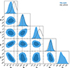Fig. 15. One- and two-dimensional marginal posterior on the parameters of the count rate–mass scaling relations from this work in blue, compared to the 1-d marginals of the analysis of HSC WL around eFEDS clusters and groups (Chiu et al. 2022) in black. We find good agreement on the mass trend BX, and the deviation from self-similar redshift scaling GX, while constraints on the amplitude AX, and the redshift evolution of the mass slope FX are shifted by 1- to 2-sigmas, consistent with statistical fluctuations. Contrary to the eFEDS-HSC analysis, we do not place an informative prior of the intrinsic scatter σX, and get only weak constraints.

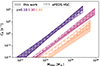Fig. 16. Posterior predictive distribution of the mean count rate–mass relation (the band ranges from the 16th to the 84th percentile at each mass), for three different redshifts (color coded). Filled bands represent the analysis in this work, and hatched bands represent the eFEDS HSC result from Chiu et al. (2022). The predictions diverge for low-mass, high-redshift systems.

5.2. Goodness of fit

To assess the goodness of fit of our mass calibration, we resort to binning the cluster sample in redshift, count rate bins, with edges (0.10, 0.19, 0.27, 0.35, 0.48, 0.8), and (0.01 0.16, 0.25, 0.30, 0.64, 20), in redshift and count rate respectively. For all clusters 𝜘 falling in each of the bins, we stack the tangential reduced shear profiles by defining the stacking weights $W_{\varkappa }={\displaystyle \sum _{b=2,3,4}{w}^b}{\displaystyle \sum _{i\in b_{\varkappa }}{w}_i^{\text{s}}}{\mathcal{R}}_i$, computing

$$\begin{array}{c}\hfill {\widehat{g}}_{\mathrm{t}}^{\mathrm{stack}}=\frac{{\sum }_{\varkappa }{W}_{\varkappa }{\widehat{g}}_{\mathrm{t},\varkappa }}{{\sum }_{\varkappa }{W}_{\varkappa }},\end{array}$$(50)

where i ∈ b_𝜘 symbolizes the sources i associated to the cluster 𝜘 in the tomographic bin b. Combining this expression with Eq. (22) shows that it is equivalent to the raw tangential reduced shear estimator in Eq. (8). Using the same weighting, we also derive the error on the stacked reduced shear

$$\begin{array}{c}\hfill {\left(\delta g_{\mathrm{t}}^{\mathrm{stack}}\right)}^2=\frac{{\sum }_{\varkappa }{W}_{\varkappa }^2\delta g_{\mathrm{t},\varkappa }^2}{{\sum }_{\varkappa }{W}_{\varkappa }^2},\end{array}$$(51)

and the mean angular separation of the source galaxies

$$\begin{array}{c}\hfill {\theta }^{\mathrm{stack}}=\frac{{\sum }_{\varkappa }{W}_{\varkappa }{\theta }_{\varkappa }}{{\sum }_{\varkappa }{W}_{\varkappa }}·\end{array}$$(52)

The resulting stacked tangential reduced shear profiles are shown as black points with their error bars in Fig. 17 given by the square root of the variance calculated above.

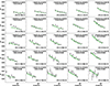Fig. 17. Stacked measured reduced tangential shear profiles with measurement uncertainty in black for different count rate (rows) and redshift (columns) bins. As a green line, the best-fit shear profile model and with filled green regions, the propagation of the posterior uncertainty on the mean model. The chosen model fits the data well at all count rates and redshifts. We also report the median WL mass of each bin in units of M⊙.

For the model prediction, we draw N_MC = 1000 points ${\mathit{p}}_{\text{SR}}^v$ from the posterior sample. For each cluster 𝜘, and for each posterior point v, we compute its best-guess WL mass

$$\begin{array}{c}\hfill M_{\mathrm{WL},\varkappa }^v=\underset{M_{\mathrm{WL}}}{\mathrm{argmax}}P(M_{\mathrm{WL}}|{\widehat{C}}_{R,\varkappa },z_{\varkappa },{\widehat{\mathcal{H}}}_{\varkappa },{\mathit{p}}_{\mathrm{SR}}^v),\end{array}$$(53)

as the maximum of the PDF of WL masses, given the count rate, redshift, and sky position, evaluated for our specific posterior draw ${\mathit{p}}_{\text{SR}}^v$. We report the median mass of the clusters in each stacking bin in Fig. 17. For each WL mass $M_{\mathrm{WL},\varkappa }^v$ we evaluate our extraction model $g_{\mathrm{t},\varkappa }^{\mathrm{mod},v}$, given in Eq. (33) using the source redshift distribution computed on the real data, Eq. (25), and the mean positions of the sources θ_α from Eq. (24). For each cluster and posterior point, we thus construct the predicted reduced shear profile as

$$\begin{array}{c}\hfill g_{\mathrm{t},\varkappa }^{\mathrm{pred},v}=(1-f_{\mathrm{RS},\varkappa }^v-f_{\mathrm{AGN},\varkappa }^v)g_{\mathrm{t},\varkappa }^{\mathrm{mod},v}+f_{\mathrm{AGN},\varkappa }^v{g}_{\mathrm{t},\varkappa }^{\mathrm{AGN}},\end{array}$$(54)

with $f_{\text{RS},\varkappa }^v$ and $f_{\text{AGN},\varkappa }^v$ the random source and AGN fractions at the count rate, redshift and sky position of the cluster 𝜘 given the model parameters ${\mathit{p}}_{\text{SR}}^v$.

The average reduced shear model in the bin is then given by stacking the predicted reduced shear profile with the same weights as the data and taking a mean over the posterior points,

$$\begin{array}{c}\hfill g_{\mathrm{t}}^{\mathrm{pred}}=\frac{1}{N_{\mathrm{MC}}}\sum _v\frac{{\sum }_{\varkappa }{W}_{\varkappa }{g}_{\mathrm{t},\varkappa }^{\mathrm{pred},v}}{{\sum }_{\varkappa }{W}_{\varkappa }},\end{array}$$(55)

and variance

$$\begin{array}{c}\hfill {\left(\delta g_{\mathrm{t}}^{\mathrm{pred}}\right)}^2=\frac{1}{N_{\mathrm{MC}}}\sum _v\frac{{\sum }_{\varkappa }{W}_{\varkappa }{(g_{\mathrm{t},\varkappa }^{\mathrm{pred},v}-g_{\mathrm{t},\varkappa }^{\mathrm{pred}})}^2}{{\sum }_{\varkappa }{W}_{\varkappa }},\end{array}$$(56)

propagating the uncertainty in the model parameters expressed by their posterior to the reduced shear profile prediction. The mean shear profile and its systematic uncertainty are shown as green lines in Fig. 17. The visual impression of a good fit is corroborated by considering that the chi-squared between stacked data and predicted model is ${\chi }^2=180.0_{-30.4}^{+45.8}$ for 150 data points and 5 parameters that are effectively constrained. The upper and lower errors for the χ² result from the difference induced when evaluating it with the model $g_{\mathrm{t}}^{\mathrm{pred}}\pm \delta g_{\mathrm{t}}^{\mathrm{pred}}$, instead of the mean model. Within the errors propagated from the posterior, we attain a very good chi-squared.

6. Discussion

6.1. Comparison to previous work

The only previous work that calibrated the eROSITA count rate – halo mass relation was performed by Chiu et al. (2022), measuring, calibrating, and analyzing the WL signal around 313 eFEDS selected clusters and groups with HSC data. Their results are shown as black lines in Fig. 15. We agree on all parameters within 2-sigma, with larger than 1-sigma deviations on the amplitude, the redshift trend of the slope and the scatter. When considering the predicted mean count rate as a function of mass and redshift, their results predict higher count rates for low-mass and high redshift objects (hatched bands in Fig. 16). The difference is, however, not statistically significant. The constraining power of this work is only marginally better than the calibration derived by Chiu et al. (2022).

The similar constraining power of eFEDS-HSC analysis to this work, despite the significantly smaller number of objects (313 compared to 2201), is explained by the higher source density in HSC and the cleaner background selection. Indeed, the signal-to-noise ratio of an individual cluster is proportional to

$$\begin{array}{c}\hfill S/N\propto \beta \sqrt{n_{\mathrm{eff}}}\sqrt{1-f_{\mathrm{cl}}},\mathrm{with}\beta =\langle \frac{min(0,D_{\mathrm{ls}})}{D_{\mathrm{s}}}{\rangle }_{P(z_{\mathrm{s}})},\end{array}$$(57)

where β is the lensing efficiency, which is 0 for sources at the lens redshift and converges to 1 for infinitely distant sources. n_eff is the effective source density, and f_cl the cluster member contamination. When considering these elements, each cluster in the HSC analysis has a WL signal-to-noise approximately a factor of 2.3 larger than the clusters considered in this work, assuming they have the same mass and ignoring cluster member contamination. Considering the overall signal-to-noise gain stemming from the total number of clusters, $\sqrt{2201/313}=2.6$, we find that it just about compensates the much lower individual clusters signal-to-noise. Note also that in the eFEDS-HSC analysis, a tighter Ω_M and an informative σ_X prior were used. Taken together, this explains the similar constraining power of the two works.

6.2. Cluster line of sight anomalies

We find several cluster line of sight anomalies that we shall discuss here cohesively. Firstly, it is somewhat anomalous that the cluster member contamination estimates based on the effective number density of sources display a larger contaminant fraction than the estimate based on the decomposition of the source redshift distribution. The latter should be impervious to masking and obstruction effects, as argued by Gruen et al. (2014), Varga et al. (2019). Estimations of the cluster member contamination via the effective number density of sources are biased low because of masking and obstruction by foreground and bright cluster sources, as shown by Kleinebreil et al. (2024). It is therefore surprising that we find the number density estimate to be larger than the source redshift distribution estimate despite it potentially being biased low. A possible source of error here is our very lenient background selection and the possible performance loss of the source redshift decomposition method if the cluster redshift lies too close to the peak of the source redshift distribution of the field. This might be hinted at by the imperfect subtraction signatures discussed in Sect. 3.3.1 and seen in Fig. 6.

Also interesting are the decrement of the effective shape noise and the increment of the smooth shear response toward the cluster center. The effect is rather constant in lens redshift, as opposed to the cluster member contamination. Indeed, we see this anomaly also in the lowest source redshift bin, 0.1 < z_l < 0.19, where we have practically no cluster member contamination. This makes it implausible that cluster member contaminants have significantly different responses or intrinsic shapes. It is worthwhile noting in Eq. (10) that a larger shear response leads to a smaller estimated effective shape noise. Also, the shear response used in this work is a smooth function of the source’s signal-to-noise and its size with respect to the PSF. Noticeably, both these quantities are magnified by the cluster’s potential – a secondary effect of WL. Such magnification effects might thus alter the inferred smooth shear response. In general, shape measurement and photo-z calibration in cluster lines of sight might be affected to second order not only by magnification but also by increased blending (Hernández-Martín et al. 2020) and the intra-cluster light (Zhang et al. 2019). Exploiting future-wide optical and NIR surveys might necessitate dedicated assessments of the performance of shape and photo-z measurement techniques in cluster lines of sight.

6.3. Impact of the mixture model

Some elements of the mixture model used to account for the residual contamination of our cluster sample (see Sect. 5.1.1) merit further discussion. Around 4.6% of our sample are found to be misclassified AGN, while another 0.6% are noise fluctuations (Bulbul et al. 2024; Kluge et al. 2024; Ghirardini et al. 2024). In both cases, we find an optical richness $\widehat{\lambda }>3$ for these objects, suggesting that they coincide with a small overdensity of red galaxies along the line of sight. Focussing on the AGN contaminants, we assume that their WL signal is sourced by an NFW with halo mass $M_{200\mathrm{c}}^{\mathrm{AGN}}=4.{95}_{1.99}^{+2.63}\times {10}^{12}{M}_{\odot }$ as measured by Comparat et al. (2023) in HSC data around eFEDS selected AGNs.

This can be contrasted with the mean halo mass ${log}_{10}{M}_{200\mathrm{m}}^{5<\widehat{\lambda }<10}\sim 14.1+{log}_{10}{M}_{\odot }$ measured by McClintock et al. (2019) for redmapper selected objects with richness $5<\widehat{\lambda }<10$ in the DES year 1 data. The latter measurement provides a weak upper bound on the halo mass of the AGN contaminants if we assume that their optical properties are equivalent to random superposition with purely optically selected clusters of similar richness. This is, however, an overestimation, as purely optically selected clusters with richness $5<\widehat{\lambda }<10$ also comprise clusters and groups that we would have selected through X-rays and thus classified as “clusters” in our mixture model, especially at low redshifts.

In the context of cosmological inference from WL calibrated cluster number counts, Ghirardini et al. (2024) have studied the impact of the mixture model in Appendix B.4. As a test, they treated the entire sample as “clusters” by setting the fraction of random source and misclassified AGN to zero. The resulting constraints on the cosmological parameters Ω_M and σ₈, the present-day amplitude of matter fluctuations on a scale of 8 h⁻¹ Mpc, are only marginally affected by this modeling choice. Both these parameters are very sensitive to the mass calibration and, thus, to the implementation of the mixture model in the context of the WL signal, which we are discussing in this paper. We therefore concluded that the modeling choices for the WL signal from the contaminants do not impact the mass calibration at a level that would be noticeable in cosmological inference.

6.4. Accounting for cluster selection biases

Much of the astrophysically driven conversation about the viability of galaxy clusters as a cosmological probe and the limits of our ability to effectively calibrate their masses focus on so-called selection biases. When taking a forward modeling approach using Bayesian population models, these concerns can be naturally accounted for. We shall discuss in the following the most (in)famous “selection bias” as an example: the “cool core bias” (Rossetti et al. 2017). The cooling time in the center of massive galaxy clusters can fall below the Hubble time, especially if they have been undisturbed for a long time. Effective cooling boosts the central luminosity, resulting in very peaked X-ray surface brightness profiles. Conversely, the SZe selection, which is sensitive to pressure, is not affected by this. As discussed already above, taking a population modeling approach immediately ensures that any sample selected on an observable that scatters around the halo mass will preferentially contain up-scattered objects compared to down-scattered objects on account of the much higher frequency of the former. If a specific physical property drives the scatter in some observable at fixed mass, a sample selected in that observable will show more objects with that physical property compared to a sample selected on another observable. X-ray-selected samples will preferentially contain objects that are scattered up in X-rays for whatever astrophysical reason.

For cosmological inference, the complication arises if the scatter in the follow-up observable used for the mass calibration correlates with the scatter in the selection observable. A glaring case being investigated is clusters selected via the number of photometric member galaxies and the WL signal of these objects. The scatter of both depends on the concentration, orientation, and triaxiality of the halo, as well as the neighboring environment, resulting in strong selection biases hampering cosmological analyses on those samples (Dark Energy Survey Collaboration 2020; Wu et al. 2022). Our analysis is unaffected by optical selection effects. While we do impose a cut of richness $\widehat{\lambda }>3$ (Kluge et al. 2024) in our analysis, this cut only leads to the exclusion of 1.1% of clusters at low redshift, low mass, and in high exposure time regions (Ghirardini et al. 2024, Appendix D) . Our selection is thus almost exclusively based on the X-ray signatures. X-ray-selected clusters have been reported to live preferentially in nodes of the cosmic web, as compared to filaments or sheets, as found by Popesso et al. (2024) when comparing eFEDS-selected halos with spectroscopically selected ones. This means that at fixed halo mass, the cluster properties may depend on secondary halo properties like environment or concentration – an effect analogous to the assembly bias of galaxies (Wu et al. 2008; Wechsler & Tinker 2018). Our scale cuts on the tangential reduced shear are designed to ensure that we measure the WL signal only in the 1-halo regime (Grandis et al. 2021a), that is, scales dominated by the halo’s own density profile and not by neighboring structures. This already limits significantly the impact of assembly bias. Still, the eRASS1 selection might correlate with some properties that also impact the WL mass, such as concentration, triaxiality, or dynamical state. To account for any such possible effect, we introduce the correlation coefficient ρ_WL, X among the scatters in count rate and WL mass. Figure 18 shows the posterior on the correlation coefficient, together with its degeneracies with the amplitude of the scaling relation and intrinsic scatter at fixed halo mass and redshift. The prior range for the correlation coefficient is naturally given by ( − 1, 1), though we sample ( − 0.9, 0.9) to avoid numerical instabilities for a singular covariance matrix. Marginalizing over the correlation coefficient makes our analysis impervious to selection bias effects but deteriorates our ability to calibrate the observable–mass relation. Given that the numerical value of the amplitude of the scaling relation directly impacts our cosmological results and, crucially, their agreement with external experiments, foregoing the use of strong astrophysical priors on the selection effects at the cost of a less stringent mass calibration is undoubtedly the more prudent choice.

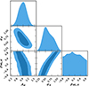Fig. 18. One- and two-dimensional marginal contours of the amplitude of the count rate–mass scaling relation AX, the intrinsic scatter around that relation σX, and the correlation coefficient between the WL and count rate scatter ρMWL, CR, labeled as ρWL, X for brevity in the plot. While the correlation coefficient remains unconstrained, it leads to significant degeneracies with the amplitude and scatter. Astrophysical processes like cluster age, merger state, environment, orientation, triaxiality, etc., might impact both observables and lead to selection biases. We agnostically marginalize over the entire range of such effects, thereby weakening our amplitude and scatter measurements but making the mass calibration impervious to such astrophysical effects.

7. Conclusions

In this work, we measured and calibrated the WL signal around eRASS1 clusters and groups in the DES Y3 data. To this end, we defined a background sample of DES galaxies by weighting tomographic redshift bins defined and calibrated for the cosmic shear experiment (Myles et al. 2021; Gatti et al. 2021) as a function of the photometric redshift of our clusters. After querying sources around our lenses, out to an angular distance corresponding to 15 h⁻¹ Mpc, we validated and calibrated that measurement. We fit the lens richness, redshift, and source-lens distance dependence of the effective source density and the source redshift distribution to determine the contamination of our source sample. The different methods employed agree with each other within the systematic uncertainties of the source redshift and shape measurement.

We fit a lens redshift trend to the effective shape noise, allowing us to define a semi-analytical covariance metric for the shape noise. The profiles of the B-mode-like cross-component are consistent with zero, as expected for a well calibrated WL signal sourced by gravity. Investigation of the selection and shear response of our tangential reduced shear estimators show that the former can be ignored, as it induces a correction much smaller than the systematic uncertainty induced by source redshift and shape measurements. On small cluster-centric distances, we find interesting anomalies in the shear response and effective shape noise that might point at cluster line-of-sight-specific calibration issues, which arguably are too small to impact our subsequent analysis steps.

We derived cosmology-ready data products to be used as inputs for the mass calibration of eRASS1 selected clusters, both in this work and self-consistently as well as in the subsequent cosmological analysis by Ghirardini et al. (2024). These products are:

• The tangential reduced shear profile in angular bins, corrected for the shear response;

• A semi-analytical estimate of the shape noise on that profile; and

• An estimate of the field source redshift distribution from the local background

for each cluster with DES Y3 lensing data. This resulted in WL data for 2201 eRASS1 selected clusters, with a raw signal-to-noise ratio of 92, reduced to 65 after our radial scale cuts are applied.

Exploitation of these data for mass calibration and number counts cosmology requires the anchoring of the mapping between halo mass and WL signal via 𝒪(1000) realizations of synthetic shear profile simulations, following the scheme presented by Grandis et al. (2021a). These simulations include:

• Realistic 2D-projected surface mass density maps around massive halos, extracted from the cosmological hydrodynamical TNG300 simulations (Pillepich et al. 2018; Marinacci et al. 2018; Springel et al. 2018; Nelson et al. 2018, 2019; Naiman et al. 2018);

• A distribution of the off-set between the observational centers used for the tangential reduced shear profile measurements, constructed from X-ray images of the MAGNETICUM PATHFINDER simulations (Dolag et al., in prep.), and the “eROSITA digital sky twin” (Seppi et al. 2022);

• A painting of the richness using the richness–mass relation calibrated by Chiu et al. (2022);

• Dilution of the tangential reduced shear signal based on the degree of cluster member contamination we calibrated;

• A noise contribution from the uncorrelated large-scale structure; and

• Realistic DES Y3 source distributions reflecting our background selection based on weighted sums of the DES Y3 tomographic redshift bins (Myles et al. 2021), together with a prescription for nonlinear shear bias.

These synthetic shear profiles were analyzed using the same shear profile model that we used in the subsequent mass calibration. It features a simplified mis-centered NFW with a fixed concentration–mass relation and accounts for the mean cluster member contamination, as advocated by Grandis et al. (2021a). It thus has one free parameter, the WL mass. Extracting the WL mass on our synthetic shear profile simulations allowed us to establish the relation between WL and halo mass, summarized in the WL bias and scatter. Monte Carlo realizations of the synthetic shear profile simulation, obtained by varying all the inputs within our expectation, resulted in an uncertainty estimate on the WL bias and scatter that acts as a calibration prior to the subsequent mass calibration. We find that at low redshift, our mass extraction uncertainty is dominated by the effect of hydrodynamical modeling, leading to a systematics floor of 2%. At higher redshifts, DES photo-z uncertainties become incrementally more important.

We calibrated the count rate to halo mass relation by using a Bayesian population model to forward model the probability density function of each cluster’s shear profile given its count rate and redshift. Improving on previous work (Mantz et al. 2016; Dietrich et al. 2019; Bocquet et al. 2019; Chiu et al. 2022), we took explicit account of contaminants via a mixture model. We find that we can measure five parameters of the count rate–mass relation: the amplitude, the slope and its redshift dependence, the deviation from a self-similar redshift evolution, and the intrinsic scatter around the relation. We assessed the quality of this population model-based fit on stacked signals in count rate and redshift bins and found excellent agreement between the data and the model. Our analysis finds comparable and marginally tighter constraints than the calibration of the eROSITA count rate–mass relation performed by Chiu et al. (2022) with HSC data on eFEDS-selected clusters.

This analysis will serve, along with similar analyses on HSC and KiDS, as the main mass calibration for the number counts of eRASS1-selected clusters (Ghirardini et al. 2024), which constrain different cosmological parameters such as the present-day matter density, the amplitude of matter fluctuations, the equation of state of dark energy, and the sum of the neutrino masses. Methodologically, we have demonstrated how photometric data from wide surveys, calibrated specifically for cosmic shear experiments, can be effectively used to perform a WL mass calibration of cluster number counts. These two experiments are highly complementary. Cosmic shear probes the large-scale structure’s linear and mildly nonlinear scale, while WL-calibrated number counts probe the most nonlinear regions and massive galaxy clusters. These probes have very different sensitivities to astrophysical and observational systematics, only sharing a joint dependence on the source photo-z and shape calibration. In light of upcoming deep and wide surveys, tailored mainly for cosmic shear, including Euclid⁵, LSST⁶, or Roman⁷, this work provides a demonstration of how to leverage these data to inform cluster number counts, enabling independent and competitive cosmological constraints.

References

- Allen, S. W., Evrard, A. E., & Mantz, A. B. 2011, ARA&A, 49, 409 [Google Scholar]
- Angulo, R. E., Springel, V., White, S. D. M., et al. 2012, MNRAS, 426, 2046 [NASA ADS] [CrossRef] [Google Scholar]
- Bahé, Y. M., McCarthy, I. G., & King, L. J. 2012, MNRAS, 421, 1073 [NASA ADS] [CrossRef] [Google Scholar]
- Becker, M. R., & Kravtsov, A. V. 2011, ApJ, 740, 25 [NASA ADS] [CrossRef] [Google Scholar]
- Bellagamba, F., Sereno, M., Roncarelli, M., et al. 2019, MNRAS, 484, 1598 [Google Scholar]
- Benítez, N. 2000, ApJ, 536, 571 [Google Scholar]
- Bleem, L. E., Bocquet, S., Stalder, B., et al. 2020, ApJS, 247, 25 [Google Scholar]
- Bocquet, S., Dietrich, J. P., Schrabback, T., et al. 2019, ApJ, 878, 55 [Google Scholar]
- Bocquet, S., Grandis, S., Bleem, L. E., et al. 2023, Phys. Rev. D, submitted [arXiv:2310.12213] [Google Scholar]
- Buchner, J. 2021, J. Open Source Softw., 6, 3001 [CrossRef] [Google Scholar]
- Bulbul, E., Liu, A., Kluge, M., et al. 2024, A&A, 685, A106 [NASA ADS] [CrossRef] [EDP Sciences] [Google Scholar]
- Castro, T., Borgani, S., Dolag, K., et al. 2021, MNRAS, 500, 2316 [Google Scholar]
- Child, H. L., Habib, S., Heitmann, K., et al. 2018, ApJ, 859, 55 [NASA ADS] [CrossRef] [Google Scholar]
- Chiu, I. N., Ghirardini, V., Liu, A., et al. 2022, A&A, 661, A11 [NASA ADS] [CrossRef] [EDP Sciences] [Google Scholar]
- Chiu, I. N., Klein, M., Mohr, J., & Bocquet, S. 2023, MNRAS, 522, 1601 [NASA ADS] [CrossRef] [Google Scholar]
- Clerc, N., Comparat, J., Seppi, R., et al. 2024, A&A, in press, https://doi.org/10.1051/0004-6361/202449447 [Google Scholar]
- Comparat, J., Merloni, A., Salvato, M., et al. 2019, MNRAS, 487, 2005 [Google Scholar]
- Comparat, J., Eckert, D., Finoguenov, A., et al. 2020, Open J. Astrophys., 3, 13 [Google Scholar]
- Comparat, J., Luo, W., Merloni, A., et al. 2023, A&A, 673, A122 [NASA ADS] [CrossRef] [EDP Sciences] [Google Scholar]
- Cordero, J. P., Harrison, I., Rollins, R. P., et al. 2022, MNRAS, 511, 2170 [NASA ADS] [CrossRef] [Google Scholar]
- Dark Energy Survey Collaboration (Abbott, T. M. C., et al.) 2019, ApJ, 872, L30 [NASA ADS] [CrossRef] [Google Scholar]
- Dark Energy Survey Collaboration (Abbott, T. M. C., et al.) 2020, Phys. Rev. D, 102, 023509 [NASA ADS] [CrossRef] [Google Scholar]
- Dark Energy Survey Collaboration (Abbott, T. M. C., et al.) 2022, Phys. Rev. D, 105, 023520 [CrossRef] [Google Scholar]
- De Vicente, J., Sánchez, E., & Sevilla-Noarbe, I. 2016, MNRAS, 459, 3078 [NASA ADS] [CrossRef] [Google Scholar]
- Dey, A., Schlegel, D. J., Lang, D., et al. 2019, AJ, 157, 168 [Google Scholar]
- Dietrich, J. P., Bocquet, S., Schrabback, T., et al. 2019, MNRAS, 483, 2871 [Google Scholar]
- Dyson, F. W., Eddington, A. S., & Davidson, C. 1920, Philos. Trans. R. Soc. Lond. Ser. A, 220, 291 [NASA ADS] [CrossRef] [Google Scholar]
- Ettori, S., Gastaldello, F., Leccardi, A., et al. 2011, A&A, 526, 1 [Google Scholar]
- Flaugher, B., Diehl, H. T., Honscheid, K., et al. 2015, AJ, 150, 150 [Google Scholar]
- Friedrich, O., Andrade-Oliveira, F., Camacho, H., et al. 2021, MNRAS, 508, 3125 [NASA ADS] [CrossRef] [Google Scholar]
- Gatti, M., Sheldon, E., Amon, A., et al. 2021, MNRAS, 504, 4312 [NASA ADS] [CrossRef] [Google Scholar]
- Ghirardini, V., Bulbul, E., Artis, E., et al. 2024, A&A, submitted [arXiv:2402.08458] [Google Scholar]
- Grandis, S., Mohr, J. J., Dietrich, J. P., et al. 2019, MNRAS, 488, 2041 [NASA ADS] [Google Scholar]
- Grandis, S., Klein, M., Mohr, J. J., et al. 2020, MNRAS, 498, 771 [NASA ADS] [CrossRef] [Google Scholar]
- Grandis, S., Bocquet, S., Mohr, J. J., Klein, M., & Dolag, K. 2021a, MNRAS, 507, 5671 [NASA ADS] [CrossRef] [Google Scholar]
- Grandis, S., Mohr, J. J., Costanzi, M., et al. 2021b, MNRAS, 504, 1253 [NASA ADS] [CrossRef] [Google Scholar]
- Gruen, D., Seitz, S., Brimioulle, F., et al. 2014, MNRAS, 442, 1507 [CrossRef] [Google Scholar]
- Haiman, Z., Mohr, J. J., & Holder, G. P. 2001, ApJ, 553, 545 [NASA ADS] [CrossRef] [Google Scholar]
- Hennig, C., Mohr, J. J., Zenteno, A., et al. 2017, MNRAS, 467, 4015 [NASA ADS] [Google Scholar]
- Hernández-Martín, B., Schrabback, T., Hoekstra, H., et al. 2020, A&A, 640, A117 [EDP Sciences] [Google Scholar]
- Hoekstra, H., Mahdavi, A., Babul, A., & Bildfell, C. 2012, MNRAS, 427, 1298 [NASA ADS] [CrossRef] [Google Scholar]
- Huff, E., & Mandelbaum, R. 2017, ArXiv e-prints [arXiv:1702.02600] [Google Scholar]
- Huterer, D. 2023, A&ARv, 31, 2 [NASA ADS] [CrossRef] [Google Scholar]
- Jarvis, M., Bernstein, G. M., Amon, A., et al. 2021, MNRAS, 501, 1282 [Google Scholar]
- Kimmig, L. C., Remus, R.-S., Dolag, K., & Biffi, V. 2023, ApJ, 949, 92 [Google Scholar]
- Kleinebreil, F., Grandis, S., Schrabback, T., et al. 2024, A&A, submitted [arXiv:2402.08456] [Google Scholar]
- Kluge, M., Comparat, J., Liu, A., et al. 2024, A&A, in press, https://doi.org/10.1051/0004-6361/202349031 [Google Scholar]
- Komatsu, E., Smith, K. M., Dunkley, J., et al. 2011, ApJS, 192, 18 [Google Scholar]
- MacCrann, N., Becker, M. R., McCullough, J., et al. 2022, MNRAS, 509, 3371 [Google Scholar]
- Majumdar, S., & Mohr, J. J. 2004, ApJ, 613, 41 [NASA ADS] [CrossRef] [Google Scholar]
- Mantz, A. B., von der Linden, A., Allen, S. W., et al. 2015, MNRAS, 446, 2205 [Google Scholar]
- Mantz, A. B., Allen, S. W., Morris, R. G., et al. 2016, MNRAS, 463, 3582 [NASA ADS] [CrossRef] [Google Scholar]
- Marinacci, F., Vogelsberger, M., Pakmor, R., et al. 2018, MNRAS, 480, 5113 [NASA ADS] [Google Scholar]
- McClintock, T., Varga, T. N., Gruen, D., et al. 2019, MNRAS, 482, 1352 [Google Scholar]
- Merloni, A., Lamer, G., Liu, T., et al. 2024, A&A, 682, A34 [NASA ADS] [CrossRef] [EDP Sciences] [Google Scholar]
- Mohr, J. J., & Evrard, A. E. 1997, ApJ, 491, 38 [Google Scholar]
- Myles, J., Alarcon, A., Amon, A., et al. 2021, MNRAS, 505, 4249 [NASA ADS] [CrossRef] [Google Scholar]
- Naiman, J. P., Pillepich, A., Springel, V., et al. 2018, MNRAS, 477, 1206 [Google Scholar]
- Navarro, J. F., Frenk, C. S., & White, S. D. M. 1996, ApJ, 462, 563 [Google Scholar]
- Nelson, D., Pillepich, A., Springel, V., et al. 2018, MNRAS, 475, 624 [Google Scholar]
- Nelson, D., Springel, V., Pillepich, A., et al. 2019, Comput. Astrophys. Cosmol., 6, 2 [Google Scholar]
- Oguri, M., & Hamana, T. 2011, MNRAS, 414, 1851 [NASA ADS] [CrossRef] [Google Scholar]
- Paulus, M. 2021, Ph.D. Thesis, Ludwig-Maximilians University of Munich, Germany [Google Scholar]
- Pillepich, A., Nelson, D., Hernquist, L., et al. 2018, MNRAS, 475, 648 [Google Scholar]
- Popesso, P., Biviano, A., Bulbul, E., et al. 2024, MNRAS, 527, 895 [Google Scholar]
- Power, C., Navarro, J. F., Jenkins, A., et al. 2003, MNRAS, 338, 14 [Google Scholar]
- Prat, J., Blazek, J., Sánchez, C., et al. 2022, Phys. Rev. D, 105, 083528 [NASA ADS] [CrossRef] [Google Scholar]
- Predehl, P., Andritschke, R., Arefiev, V., et al. 2021, A&A, 647, A1 [EDP Sciences] [Google Scholar]
- Ragagnin, A., Saro, A., Singh, P., & Dolag, K. 2021, MNRAS, 500, 5056 [Google Scholar]
- Rossetti, M., Gastaldello, F., Eckert, D., et al. 2017, MNRAS, 468, 1917 [Google Scholar]
- Rozo, E., Rykoff, E. S., Becker, M., Reddick, R. M., & Wechsler, R. H. 2015, MNRAS, 453, 38 [NASA ADS] [CrossRef] [Google Scholar]
- Rykoff, E. S., Rozo, E., Busha, M. T., et al. 2014, ApJ, 785, 104 [Google Scholar]
- Rykoff, E. S., Rozo, E., Hollowood, D., et al. 2016, ApJS, 224, 1 [NASA ADS] [CrossRef] [Google Scholar]
- Saro, A., Bocquet, S., Rozo, E., et al. 2015, MNRAS, 454, 2305 [Google Scholar]
- Schneider, P., 2006, in Saas-Fee Advanced Course 33: Gravitational Lensing: Strong, Weak and Micro, eds. G. Meylan, P. Jetzer, P. North, et al., 269 [NASA ADS] [CrossRef] [Google Scholar]
- Schrabback, T., Bocquet, S., Sommer, M., et al. 2021, MNRAS, 505, 3923 [NASA ADS] [CrossRef] [Google Scholar]
- Seppi, R., Comparat, J., Bulbul, E., et al. 2022, A&A, 665, A78 [NASA ADS] [CrossRef] [EDP Sciences] [Google Scholar]
- Sevilla-Noarbe, I., Bechtol, K., Carrasco Kind, M., et al. 2021, ApJS, 254, 24 [NASA ADS] [CrossRef] [Google Scholar]
- Sheldon, E. S., & Huff, E. M. 2017, ApJ, 841, 24 [NASA ADS] [CrossRef] [Google Scholar]
- Shin, T., Jain, B., Adhikari, S., et al. 2021, MNRAS, 507, 5758 [NASA ADS] [CrossRef] [Google Scholar]
- Sommer, M. W., Schrabback, T., Ragagnin, A., & Rockenfeller, R. 2023, MNRAS, submitted [arXiv:2306.13187] [Google Scholar]
- Song, J., Zenteno, A., Stalder, B., et al. 2012, ApJ, 761, 22 [NASA ADS] [CrossRef] [Google Scholar]
- Springel, V., Pakmor, R., Pillepich, A., et al. 2018, MNRAS, 475, 676 [Google Scholar]
- Story, K., Aird, K. A., Andersson, K., et al. 2011, ApJ, 735, L36 [NASA ADS] [CrossRef] [Google Scholar]
- Sunayama, T. 2023, MNRAS, 521, 5064 [NASA ADS] [CrossRef] [Google Scholar]
- Sunayama, T., Park, Y., Takada, M., et al. 2020, MNRAS, 496, 4468 [CrossRef] [Google Scholar]
- Sunyaev, R., Arefiev, V., Babyshkin, V., et al. 2021, A&A, 656, A132 [NASA ADS] [CrossRef] [EDP Sciences] [Google Scholar]
- Umetsu, K. 2020, A&ARv, 28, 7 [Google Scholar]
- Varga, T. N., DeRose, J., Gruen, D., et al. 2019, MNRAS, 489, 2511 [NASA ADS] [CrossRef] [Google Scholar]
- Wechsler, R. H., & Tinker, J. L. 2018, ARA&A, 56, 435 [NASA ADS] [CrossRef] [Google Scholar]
- Wu, H.-Y., Rozo, E., & Wechsler, R. H. 2008, ApJ, 688, 729 [Google Scholar]
- Wu, H.-Y., Costanzi, M., To, C.-H., et al. 2022, MNRAS, 515, 4471 [CrossRef] [Google Scholar]
- Zhang, Y., Yanny, B., Palmese, A., et al. 2019, ApJ, 874, 165 [Google Scholar]
- Zohren, H., Schrabback, T., Bocquet, S., et al. 2022, A&A, 668, A18 [NASA ADS] [CrossRef] [EDP Sciences] [Google Scholar]
Appendix A: Effective shape noise and number density in the presence of shear responses
The aim of this appendix is to present a derivation for the expression of the effective shape variance, Eq. 10 and the effective number density, Eq. 9, in the presence of a shear response ℛ.
Friedrich et al. (2021) demonstrate that the variance of a reduced shear profile  is given by
![Mathematical equation: $$ \begin{aligned} \mathrm{Var}\left[ \hat{g}_{\rm t}\right] = \frac{\sigma ^2_{\rm eff}}{N_{\rm pair}}~\mathrm{with}~\sigma ^2_{\rm eff}=\frac{1}{2 N_{\rm s}} \sum |e|^2 { w}_{\rm n}^2, \end{aligned} $$](/articles/aa/full_html/2024/07/aa48615-23/aa48615-23-eq125.gif) (A.1)
(A.1)
where Npair is the number of source lens pairs, Ns the number of sources,  the squared modulus of the ellipticity when interpreted as a complex number, and wn normalized weights.
To generalize this expression to un-normalized weight w, just consider that such un-normalized weights can always be rescaled to normalized weights with the ansatz wn = Cw. The normalization condition then readily leads to an expression for C, reading
(A.2)
Moving into the regime of individual cluster lensing, where Npair = Ns, combining all the above equations, we find
![Mathematical equation: $$ \begin{aligned} \mathrm{Var}\left[ \hat{g}_{\rm t}\right] = \frac{1}{2} \frac{1}{\left( \sum { w} \right)^2} \sum |e|^2 { w}^2, \end{aligned} $$](/articles/aa/full_html/2024/07/aa48615-23/aa48615-23-eq128.gif) (A.3)
(A.3)
for generic, un-normalized weights.
When considering shear data with shear responses ℛ, Friedrich et al. (2021), Appendix D suggests transforming the above equations by re-scaling both the ellipticities e, as well as the weight w, as follows
(A.4)
thus correcting the ellipticity for the shear response and adjusting the weights for the necessary re-scaling. Note that the summand in the numerator of Eq. A.3 is invariant under this re-scaling,  , and we thus only have to modify the summand in the denominator. Given that the above expression is valid for un-normalized weights, no further corrections are required.
Dropping the tildes, we can readily write the variance of a tangential reduced shear profile in the presence of shear response as
![Mathematical equation: $$ \begin{aligned} \mathrm{Var}\left[ \hat{g}_{\rm t}\right] = \frac{1}{2} \frac{1}{\left( \sum { w} \mathcal{R} \right)^2} \sum |e|^2 { w}^2. \end{aligned} $$](/articles/aa/full_html/2024/07/aa48615-23/aa48615-23-eq131.gif) (A.5)
(A.5)
Similarly, this justifies also why the source redshift distribution needs to be shear response weighted.
Interpreting this expression as the ratio between an effective shape dispersion σeff, α for α∈ (t, x), and an effective number of source Neff we can recover the above expression by using
(A.6)
which are the expressions that we also use for our shape noise modeling.
Appendix B: Parametrisation of cluster member contamination
We shall justify in the following the parameterization used for the cluster member contamination in Section 3.3.1. As shown by Hennig et al. (2017), cluster member galaxies follow an NFW profile, with the total number of galaxies enclosed in the virial region correlating tightly with mass, while the concentration varies depending on the galaxy type. Red-sequence galaxies have a larger concentration, which is more similar to the concentration of dark matter than non-red-sequence galaxies. We therefore assumed that the cluster member galaxies that contaminated our background sample also follow an NFW profile.
The fraction of red-sequence galaxies in the cluster member contamination is unknown, though it stands to argue that their more precise photometric redshifts make it easier to exclude them with a background selection. We therefore let the concentration c of the cluster member contaminants profile as a free parameter.
Similarly, we choose an agnostic approach to the redshift trend of the cluster member contamination. We simply assume that the ratio between the number density of field galaxies nfield(z) and cluster member contaminants is a smooth function of redshift. We therefore employ a non-parametric fit of the amplitudes Azi for pivot redshifts zi.
To account for possible mass trends, we use the richness λ as a mass proxy, given that we have to fit for the cluster member contamination prior to performing a mass calibration and therefore do not have WL-calibrated mass estimates at our disposal. For ICM-selected cluster samples, richness is known to scale approximately linearly with halo mass, λ ∼ M (Saro et al. 2015; Bleem et al. 2020; Grandis et al. 2020, 2021b). We therefore used the richness to define an approximate virial radius for the NFW profile of the cluster member contaminants as Rvir ∝ (λ/20)1/3. We also allowed the amplitude of the cluster member contamination to vary with richness.
Taken together, the above considerations lead to the ansatz
(B.1)
The total number density results from the sum of the cluster member contaminants’ number density and the field number density as
![Mathematical equation: $$ \begin{aligned} n_{\rm tot} = n_{\rm fcl}(\lambda , z, R) + n_{\rm field}(z) = \left[ A(\lambda , z, R)+1 \right] n_{\rm field}(z), \end{aligned} $$](/articles/aa/full_html/2024/07/aa48615-23/aa48615-23-eq134.gif) (B.2)
(B.2)
while the fraction of cluster member contaminants is
(B.3)
thus justifying the parametrisation chosen in Eq. 12. This parametrization has the benefit that for A(λ, z, R) > 0, 0 < fcl(λ, z, R) < 1, as already noted by Grandis et al. (2021b) in the context of the richness-dependent contamination of photometrically selected cluster samples.
Finally, one can show that 1 + A = (1 − fcl)−1, thus also motivating Eq. 14.
All Tables
Overview of the simulation inputs used for the calibration of the WL bias and scatter.
Calibration parameters with their priors for the Monte Carlo marginalization of the WL bias and scatter determination.