| Issue |
A&A
Volume 687, July 2024
|
|
|---|---|---|
| Article Number | A242 | |
| Number of page(s) | 14 | |
| Section | Extragalactic astronomy | |
| DOI | https://doi.org/10.1051/0004-6361/202449369 | |
| Published online | 22 July 2024 | |
Comprehensive view of a z ∼ 6.5 radio-loud quasi-stellar object: From the radio to the optical/NIR to the X-ray band
1
INAF, Osservatorio Astronomico di Brera, Via Brera 28, 20121 Milano, Italy
e-mail: luca.ighina@inaf.it
2
DiSAT, Università degli Studi dell’Insubria, Via Valleggio 11, 22100 Como, Italy
3
International Centre for Radio Astronomy Research, Curtin University, 1 Turner Avenue, Bentley, WA 6102, Australia
4
SKA Observatory, Science Operations Centre, CSIRO ARRC, 26 Dick Perry Avenue, Kensington, WA 6151, Australia
5
CSIRO Space & Astronomy, PO Box 1130 Bentley, WA 6102, Australia
6
Sydney Institute for Astronomy, School of Physics, University of Sydney, NSW 2006, Australia
7
CSIRO Space and Astronomy, PO Box 76 Epping, NSW 1710, Australia
8
ARC Centre of Excellence for Gravitational Wave Discovery (OzGrav), Hawthorn, VIC 3122, Australia
9
David A. Dunlap Department of Astronomy and Astrophysics, University of Toronto, 50 St. George St., Toronto, Ontario M5S3H4, Canada
10
Racah Institute of Physics, The Hebrew University of Jerusalem, Jerusalem 91904, Israel
11
INFN, Sezione di Milano-Bicocca, Piazza della Scienza 3, 20126 Milano, Italy
12
Max Planck Institut für Astronomie, Königstuhl 17, 69117 Heidelberg, Germany
13
INAF – Osservatorio di Astrofisica e Scienza dello Spazio (OAS), Via Gobetti 93/3, 40129 Bologna, Italy
14
ATNF, CSIRO Space & Astronomy, PO Box 1130 Bentley, WA 6102, Australia
Received:
28
January
2024
Accepted:
22
April
2024
We present a multi-wavelength analysis, from the radio to the X-ray band, of the redshift z = 6.44 VIK J2318−31 radio-loud quasi-stellar object, one of the most distant currently known of this class. The work is based on newly obtained observations (uGMRT, ATCA, and Chandra) as well as dedicated archival observations that have not yet been published (GNIRS and X-shooter). Based on the observed X-ray and radio emission, its relativistic jets are likely young and misaligned from our line of sight. Moreover, we can confirm, with simultaneous observations, the presence of a turnover in the radio spectrum at νpeak ∼ 650 MHz that is unlikely to be associated with self-synchrotron absorption. From the near-infrared spectrum we derived the mass of the central black hole,  , and the Eddington ratio,
  , using broad emission lines as well as an accretion disc model fit to the continuum emission. Given the high accretion rate, the presence of a ∼8 × 10⁸ M⊙ black hole at z = 6.44 can be explained by a seed black hole (∼104 M⊙) that formed at z ∼ 25, assuming a radiative efficiency ηd ∼ 0.1. However, by assuming ηd ∼ 0.3, as expected for jetted systems, the mass observed would challenge current theoretical models of black hole formation.
Key words: galaxies: high-redshift / galaxies: jets / galaxies: nuclei / quasars: general / quasars: supermassive black holes / quasars: individual: VIK J2318−31
© The Authors 2024
 Open Access article, published by EDP Sciences, under the terms of the Creative Commons Attribution License (https://creativecommons.org/licenses/by/4.0), which permits unrestricted use, distribution, and reproduction in any medium, provided the original work is properly cited.
This article is published in open access under the Subscribe to Open model. Subscribe to A&A to support open access publication.
1. Introduction
High-redshift quasi-stellar objects (QSOs) are among the most important tools for investigating the properties of supermassive black holes (SMBHs) in the initial stages after their formation (e.g., Volonteri et al. 2021). In particular, the observation of very massive black holes (BHs) already at z ∼ 6 − 7, that is, 900–750 Myr after the Big Bang, has challenged our current understanding of BH formation and growth (e.g., Pacucci et al. 2017). In order to produce ∼108 − 9 M⊙ BHs in such a short period of time, they must originate from already massive seed BHs through the direct collapse of low-metallicity gas clouds (∼105 − 6 M⊙; e.g., Oh & Haiman 2002; Ferrara et al. 2014; Maio et al. 2019) or through stellar-dynamical interactions in dense primordial star clusters (∼103 − 4 M⊙; e.g., Devecchi & Volonteri 2009; Sakurai et al. 2017). Otherwise, in the case of a relatively low-mass seed BH produced by, for example, the collapse of Population III stars (∼102 − 3 M⊙; e.g., Banik et al. 2019), super-Eddington accretion must occur in the first phases of the SMBH evolution (e.g., Pezzulli et al. 2016; Takeo et al. 2019). Even more challenging to explain is the presence of very massive BHs hosted in radio-loud (RL)1 QSOs at z > 6. These systems are able to expel part of the accretion matter in the form of two bipolar relativistic jets (e.g. Padovani 2017), which can extend up to mega-parsec scales (e.g. Bagchi et al. 2014; Mahato et al. 2022). The presence of relativistic jets is usually associated with highly spinning BHs (e.g. Blandford & Znajek 1977; Blandford et al. 2019), which have a higher radiative efficiency (ηd ∼ 0.3; e.g. Thorne 1974) compared to radio-quiet (RQ) QSOs (i.e. QSOs without relativistic jets; ηd ∼ 0.1). This would imply either that RL QSOs originate from the most massive seed BHs or that they must be accreting at a super-Eddington rate. In order to constrain the effect that relativistic jets have on the accretion and evolution of the SMBHs that host them, statistical samples of high-z RL QSOs with multi-wavelength information are needed. While optical and infrared (IR) observations are crucial for investigating the accretion process and constraining the properties of the central SMBH (e.g. Shen et al. 2019; Farina et al. 2022; Mazzucchelli et al. 2023), radio and X-ray data can be used to characterise the relativistic jets (e.g. An et al. 2020; Spingola et al. 2020; Ighina et al. 2022b).
Even though the number of known z > 6 RL QSOs is limited to a handful of sources (e.g., McGreer et al. 2006; Willott et al. 2010), recent efforts have significantly increased the number of known RL sources at high redshifts (e.g., Belladitta et al. 2020; Bañados et al. 2021), including obscured radio QSOs (e.g., Drouart et al. 2020; Endsley et al. 2022, 2023), potentially up to z ∼ 7.7 (Lambrides et al. 2024). The discovery of many z > 6 RL QSOs has also been possible thanks to the recent advent of new-generation radio surveys. Two examples of such surveys are the LOFAR Two-metre Sky Survey (LoTSS; Shimwell et al. 2017, 2019, 2022) and the Rapid ASKAP Continuum Survey (RACS: McConnell et al. 2020; Hale et al. 2021; Duchesne et al. 2023). Both these surveys enabled the radio detection of already known high-z QSOs as well as the discovery of new ones (see e.g., Gloudemans et al. 2021, 2022 for LOFAR and Ighina et al. 2021, 2023 for RACS).
In particular, in Ighina et al. (2021), we were able to uncover the RL nature of the z = 6.44 QSO VIKING J231818.3−311346 (hereafter VIK J2318−31) thanks to the first data release of the RACS-low survey, at 888 MHz (McConnell et al. 2020). Being one of the most distant RL QSOs currently known, the characterisation of VIK J2318−31 and the other few similar sources in this redshift range can provide more stringent constraints on the evolution of SMBHs hosted in RL systems than the majority of the other sources in this class. Moreover, in Ighina et al. (2022a), by combining radio observations of the Galaxy And Mass Assembly (GAMA; Driver et al. 2011) 23h field, where VIK J2318−31 is located, we constrained its radio spectrum over two orders of magnitudes in frequency (∼0.1–10 GHz observed, corresponding to ∼0.7–75 GHz in the rest frame). Based on the shape of the radio spectrum and its variability at 888 MHz, we found that this system likely hosts a young radio jet with a projected size of the order of 1 milliarcsecond (mas; ∼5–10 pc). Similar conclusions were also drawn from very long baseline interferometry observations (Zhang et al. 2022), in which the source is only partially resolved on scales of ∼2 mas.
In this work we present a multi-wavelength study of this source, covering the radio, optical/IR, and X-ray bands. The work is based on newly obtained observations as well as archival ones not yet published. In Sect. 2 we describe the data underlying this work. In Sect. 3 we use radio and X-ray observations to constrain the properties of the relativistic jets and optical/near-infrared (NIR) observations to estimate the mass of the central BH. Finally, we summarise our results in Sect. 4.
Throughout the paper we assume a flat Lambda cold dark matter cosmology with H0 = 70 km s−1 Mpc−1, ΩM = 0.3, and ΩΛ = 0.7, where 1″ corresponds to a projected distance of 5.49 kpc at z = 6.44. Spectral indices are given assuming Sν ∝ ν−α, and all errors are reported at 68% confidence levels unless specified otherwise.
2. Multi-wavelength data
VIK J2318−31 has already been targeted with several radio observations, described in Ighina et al. (2022a) and Zhang et al. (2022), as well ALMA observations (see Decarli et al. 2018; Venemans et al. 2020, and Neeleman et al. 2021). In this section, we describe datasets that have not been published yet in the X-ray, radio and optical/NIR bands.
2.1. X-ray: Chandra
VIK J2318−31 was observed with the Chandra X-ray telescope during Cycle 23 for a total of 70 ks (project 704300, P.I. L. Ighina). Data reduction was performed using the Chandra Interactive Analysis of Observations (CIAO; Fruscione et al. 2006) software package (v4.13) with CALDB (v4.9.5). We used the SPECEXTRACT task in order to extract the photons from a 2″ region centred on the optical/NIR position of the QSO, while the background photon counts from a 10−25″ annulus, again centred at the optical/NIR position of the QSO (see Fig. 1). The source is detected with 12 net photons over an expected background of ∼1 photon. We then analysed the extracted photons using the XSPEC (v12.11.1) package and performed a fit adopting the C-statistic (Cash 1979) in the energy range 0.5–7 keV (in order to reduce the background noise) with a power law absorbed by the Galactic column density along the line of sight (NH = 1.13 × 1020 cm−2; HI4PI Collaboration 2016). In particular, we considered both a model where the photon index value was fixed to Γ = 2.0 (as typically observed in 0 < z < 6 QSOs; see e.g., Vignali et al. 2005; Piconcelli et al. 2005; Nanni et al. 2017) and one where it was free to vary. We report in Table 1 and Fig. 1 the results of the analysis, together with the  parameter value, following Ighina et al. (2019). This parameter is defined as
  log
log and is meant to quantify the relative emission in the X-rays, produced by the jets and/or the X-ray corona, compared to the optical one, associated with the accretion disc (AD).
  is related to the commonly used αox, defined at 2 keV instead of 10 keV, as
  .
.
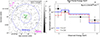 |
Fig. 1. X-ray observations of VIK J2318−31. Left: X-ray image of VIK J2318−31 from a 70 ks Chandra observation. The extraction region for the target and background spectra are reported as a solid green circle and a dotted blue annulus. Right: X-ray spectrum of VIK J2318−31. The best-fit power law spectra obtained using the cstat statistics are reported as a solid blue line (with Γ as a free parameter) and as a dashed-dotted red line (with Γ fixed). The corresponding best-fit values are reported in Table 1. |
Best-fit values obtained from the fit of the X-ray spectrum of VIK J2318−31 assuming a simple power law with Galactic absorption (NH = 1.13 × 1020 cm−2; HI4PI Collaboration 2016).
2.2. Radio observations
In Ighina et al. (2022a) we constrained the radio emission of VIK J2318−31 using multi-wavelength data obtained as part of surveys or dedicated observations. However, we note that, after a more detailed analysis of the 888 MHz ASKAP image of the G23 field taken in March 2019, Gürkan et al. (2022) corrected the flux density of VIK J2318−31 to be S888 MHz = 0.68 ± 0.07 mJy beam−1 with respect to the one we reported in Ighina et al. (2021, 2022a). In the following, we adopt the updated value from Gürkan et al. (2022).
Moreover, after the publication of Ighina et al. (2022a), more observations of the G23 field have been performed at 216 MHz with the Murchinson Widefield Array (MWA; Tingay et al. 2013) as part of the MWA Interestingly Deep AStrophysical Survey (MIDAS; Paterson et al., in prep.). This new 216 MHz image uses 1701 2-min snap-shot observations (compared to the 154 used in the pilot MIDAS image previously described in Quici et al. 2021). Additionally, an improved pipeline has been used for the new analysis that calibrates from the GaLactic and Extra-Galactic All-sky MWA (GLEAM; Wayth et al. 2015; Hurley-Walker et al. 2017) survey and also processes the two polarisations separately. Numerous improvements are incorporated for this ultra-deep MWA field with full details available in Paterson et al. (in prep.). We report in Fig. A.1 the cutout of these observations around VIK J2318−31 where an RMS of 0.28 mJy beam−1 is reached (with respect to 0.45 mJy beam−1 reported in Ighina et al. 2022a). As this new MWA image is close to being confusion limited, this new RMS is measured by fitting a Gaussian to the peak of the pixel distribution. Interestingly, VIK J2318−31 is still not detected even in this new, deeper image (although the peak flux is 0.51 mJy beam−1 = 1.8 × σ). The flux scale is accurate to ∼5% with respect to GLEAM from cross-matching of bright and isolated sources. We included this value, added in quadrature, when computing the 3σ upper limit for the low-frequency radio emission of VIK J2318−31 (see Table 2).
Best-fit flux densities obtained from a Gaussian fit to the radio images of VIK J2318–31 together with the synthesised beam size, position angle (PA), and RMS of each observation.
Dedicated upgraded Giant Metrewave Radio Telescope (uGMRT) observations of VIK J2318−31 (project 42_001; P.I. L. Ighina) were performed in two different seven hour epochs: 2022 April 22 and 2022 September 02. In both epochs the target was observed in band-3 (centred at 400 MHz) and in band-4 (centred at 650 MHz) using the GMRT wideband backend (Reddy et al. 2017). During each run, we observed sources 3C48 and 0025−260 as primary and secondary calibrators, respectively. For the data reduction of these observations we used the CAsa Pipeline-cum-Toolkit for Upgraded GMRT data REduction (CAPTURE; Kale & Ishwara-Chandra 2021) code, which is based on the Common Astronomy Software Applications (CASA) package (McMullin et al. 2007), and applied further flagging when needed. In particular, during the imaging part, which relies on the tCLEAN task, we adopted a robust parameter of 0.5. We present the images obtained in Fig. A.2 and the results of the 2D Gaussian fit (with CASA) in Table 2. We considered a further 5% in the uncertainties (added in quadrature) of the measurements derived from these images in order to account for the uncertainty related to the calibration process.
Similarly to uGMRT, Australia Telescope Compact Array (ATCA) observations were performed in two epochs (project C3477; P.I. L. Ighina) of 12 hours each and simultaneous to the uGMRT ones: 2022 April 22 (configuration 1.5A) and 2022 September 02 (configuration 6D). Observations were carried at 2.1, 5.5, and 9 GHz using the Compact Array Broadband Backend (CABB; Wilson et al. 2011), with a nominal bandwidth of 2048 MHz (divided into channels of 1 MHz). We used the source PKS B1934−638 as the standard primary calibrator (Reynolds 1994), observed at the beginning of each session, and J2255−282 as secondary calibrator, alternating its observations with the target in order to ensure the phase calibration throughout the runs. To process the data (calibration and imaging), we used the MIRIAD data-reduction package (Sault et al. 1995) following a standard reduction. In particular, for imaging, we adopted a robust parameter of 0.5. Finally, we performed a 2D Gaussian fit on the target using CASA. The final images are reported in Fig. A.3. VIK J2318−31 is detected in all the observations apart from the September run at 9 GHz. Moreover, the signal-to-noise ratio (S/N) in the 9 GHz image from April is not high enough to perform a fit to the source. Therefore, in this last case we only report the peak emission. We show the results of the fits in Table 2, where we also considered a conservative 5% (added in quadrature) in the errors of these ATCA measurements in order to account for the uncertainty related to the calibration process. We note that the different sensitivities reached during the two observing runs are mainly due to poor weather conditions during the September run, which affected the higher frequencies more. In particular, during the September run the median seeing was a factor of ∼1.5 larger than in the April run (240 μm and 160 μm, respectively). At the same time, the more extended configuration in the September run significantly reduced radio frequency interference at 2.1 GHz, thus increasing the sensitivity at this frequency compared to the previous run. In all the images, the source is unresolved.
2.3. Optical/NIR: X-shooter and GNIRS
Archival optical/NIR spectroscopic observation with X-shooter (Very Large Telescope; Vernet et al. 2011) and with the Gemini Near-Infrared Spectrograph (GNIRS; Gemini-North Telescope; Elias et al. 2006b,a) of VIK J2318−31 are available. The target was observed with GNIRS for a total of 1 h (12 segments of 300 s each) with a 1″ slit (programme ID GN-2013B-Q-50, P.I. K. Chambers) on the 2013 September 30. Moreover, the source was observed for a total of 2.7 h with X-shooter (8 segments of 1200 s each) with a 0.9″ and 0.6″ slit for the OPT and NIR arm, respectively (programme ID 097.B-1070, P.I. Farina), half performed on 2016 August 05 and half on the 2016 August 25. For the data reduction of the X-shooter VIS data, we used the ESOReflex workflow (Freudling et al. 2013). For the data reduction of the GNIRS and X-shooter-NIR observations we used the Python Spectroscopic Data Reduction Pipeline (PypeIt) Python package (Prochaska et al. 2020b,a; see e.g., Bañados et al. 2021, 2023 for applications to similar objects). In particular, we only considered half of the X-shooter-NIR segments (from the 2016 August 05 run) since during the other half the seeing was significantly worse (1.2″) with respect to the first run (0.6″) and the loss in flux, for an already faint target, was too severe for an optimal spectrum extraction. We extracted 1D spectra from each observing segment, we combined the spectra from the same instrument and then fitted a telluric model based on the grids from the line-by-line radiative transfer model LBLRTM4 (Clough et al. 2005; Gullikson et al. 2014). In order to have a consistent absolute flux calibration, we normalised both the GNIRS and X-shooter-NIR spectrum to the VIKING-band-J magnitude, while the X-shooter-VIS spectrum was normalised to the VIKING-band-Z magnitude. Both magnitudes have been corrected for Galactic extinction assuming RV = 3.1 (Schlafly & Finkbeiner 2011) and the extinction law from Fitzpatrick (1999). In both cases the corrections were Δmag < 0.02. We then re-binned the spectra to a common wavelength grid with a pixel size of 250 km s−1 using the SpectRes: Simple Spectral Resampling (SpecRes) code (Carnall 2017) and we averaged them using the inverse variance of each spectrum as weight. We show the spectrum obtained in Fig. 2, where we removed the wavelengths affected by heavy telluric absorption. In the following we adopt the redshift derived from the [CII] emission line (158 μm, rest frame) observed in ALMA as the most reliable estimate: 6.4429 ± 0.0003 (Venemans et al. 2020).
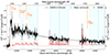 |
Fig. 2. NIR spectrum of VIK J2318−31 obtained from GNIRS+X-shooter observations (black continuum line). The spectrum was re-binned to a resolution of 250 km s−1. The dotted red line indicates the error on the spectrum. The regions affected by strong telluric absorption have been masked. The cyan shaded areas indicate the wavelength regions used to derive the photometric points (cyan circles) used for the accretion model fit. The dashed orange lines indicate the expected wavelength of the brightest emission lines present in the observed spectrum. |
3. Multi-wavelength properties
VIK J2318−31 is one of the very few RL QSOs at z > 6 for which observations along the entire electromagnetic spectrum are available. In the following, we discuss its properties based on the multi-wavelength data described in the previous section.
3.1. X-ray emission
The X-ray emission in RL QSOs is a useful tool for assessing the orientation of their relativistic jets, or in other words, their blazar nature (e.g., Ghisellini 2015). Indeed, if one of the relativistic jets is oriented close to our line of sight (i.e., in the blazar case), we expect relativistic beaming effects to significantly increase the X-ray emission (even more than the radio one; e.g., Ghisellini 2013) as well as to produce a ‘flat’ X-ray spectrum (Γ ≲ 1.7; e.g., Ighina et al. 2019; Paliya et al. 2020). Based on the best-fit parameters derived for VIK J2318−31 (see Table 1), its relativistic jets are unlikely to be oriented close to our line of sight. Indeed, a best-fit photon index value of  and an X-ray-to-optical ratio
  (or
(or  , assuming Γ = 2.0 ± 0.5) are significantly larger than what is normally observed in blazars, even at high redshifts (Γ ≲ 1.7 and
  ; see e.g., Ighina et al. 2019). Moreover, the overall X-ray luminosity is fully consistent with the one expected from the L2500 Å−LX relation derived by Lusso & Risaliti (2016) (assuming Γ = 2; see Fig. 3) and then also confirmed at high redshift (e.g., Vito et al. 2019; Salvestrini et al. 2019). It is therefore likely that the X-ray emission observed in VIK J2318−31 is dominated by the X-ray corona rather than a relativistic jet.
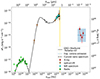 |
Fig. 3. Rest-frame spectral energy distribution, from the radio to the X-ray band, of VIK J2318−31. Radio data are reported as green squares together with the best-fit curved radio spectrum derived (dashed black line); optical and IR data from the literature are reported as brown inverted triangles, while the photometric points used for the AD model are reported as cyan circles; the X-ray Chandra data are reported as red diamonds together with the expected X-ray emission from the LX−L2500 Å relation derived in Lusso & Risaliti (2016) (assuming Γ = 2; blue shaded region). The shaded yellow area represents the range of optical frequencies where the Lyα absorption from the intergalactic medium takes place. |
At the same time, by considering the bolometric luminosity of VIK J2318−31 derived from the optical emission (Lbol = 8.4 ± 2.8 × 1046 erg s−1; see Sect. 3.3), we can compute the X-ray bolometric correction associated with the VIK J2318−31 system, defined as the ratio KX = Lbol/L2−10 keV. In this way, we obtain KX ∼ 50 − 90 (depending on the value of Γ assumed), which is consistent with the value derived, for example, by Shen et al. (2020) ( ). Once again, this suggests that the contribution from the relativistic jet to the observed X-ray emission in VIK J2318−31 is only marginal.
3.2. Radio properties
In our previous studies focused on the radio properties of VIK J2318−31, we found that the radio spectrum shows a flattening at lower frequencies and signs of variability at 888 MHz (∼2.5σ previously reported and reduced to ∼2σ with the new analysis of the GAMA 23 field; Gürkan et al. 2022). In Fig. 4 we present all the radio measurements available for VIK J2318−13 from Ighina et al. (2022a) together with the new data discussed in Sect. 2. From the newly obtained simultaneous observations with ATCA and uGMRT, we do not find any further variability in the observed range of 0.4–9 GHz: all the measurements are consistent within ∼2σ. At the same time, these uGMRT+ATCA simultaneous radio data ultimately confirm the presence of a flattening of the radio spectrum at low frequencies. Therefore, similarly to Ighina et al. (2022a), we performed a fit, in the rest frame, to all the radio data points (Fig. 4) using the MrMOOSE code (Drouart & Falkendal 2018b,a) with a curved radio spectrum of the form
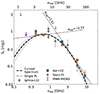 |
Fig. 4. Radio spectrum of VIK J2318−31. Data already presented in Ighina et al. (2022a) are shown as grey pentagons, while new observations are reported as blue squares (April epoch) and orange circles (September epoch). The purple upper-limit is the estimate derived from the new MWA-MIDAS image. The dashed black line shows the best-fit curved spectrum described in the text. The shaded grey area encloses the curves obtained by varying the best-fit parameters by ±1σ. The dashed line shows the best-fit double power law, while the dotted lines are the best-fit single power law describing the data above and below 1.4 GHz in the observed frame. |
where N is the normalisation, α is the index of the power law and the q parameter is a measurement of the curvature of the spectrum (|q|> 0.2 indicates a significantly curved spectrum; Callingham et al. 2017). The peak frequency of the spectrum is given by νpeak = e−α/2q. In this way we obtained q = 0.44 ± 0.4 and α = 0.38 ± 0.06, which result in a peak frequency of νpeak = 650 ± 60 MHz, consistent with the values previously found. Even though in Ighina et al. (2022a) we also discussed the possibility of a double power law as a potential radio spectral model due to the cooling of the most energetic electrons with the jets on timescales of 104 − 5 yr, recent Very Large Baseline Array (VLBA) observations of VIK J2318−31 revealed that the radio emission is very compact (∼2 mas) and, therefore, likely associated with a very young radio jet (see Zhang et al. 2022), with a kinematic age of ∼200 yr (assuming an expansion velocity of ∼0.2 c; e.g., An & Baan 2012).
Nevertheless, in order to ease the comparison of our source with other high-z sources from the literature with a more limited frequency coverage, we also performed a fit to the radio spectrum of VIK J2318−31 considering two single power laws, describing the emission at frequencies above and below ∼1.4 GHz in the observed frame. In this way we obtained a spectrum with αlow = −0.13 ± 0.09 for ν ≲ 1 GHz and with αhigh = 1.51 ± 0.11 at larger frequencies (see Fig. 4). These values are similar to what is normally found in other z > 5 radio objects, both in the 0.14 − 1.4 GHz frequency range (e.g., Gloudemans et al. 2021) as well as at ∼1.4 − 10 GHz (e.g., Drouart et al. 2020; Shao et al. 2022). Also in this case, the different signs of the spectral indexes at low and high frequencies indicate the presence of a turnover in the radio spectrum of VIK J2318−31 around ∼1 GHz in the observed frame. As described below, such a peak can be understood as due to synchrotron self-absorption (SSA) and/or free–free absorption (FFA).
Having an estimate of the turnover frequency as well as the linear size of the radio source (from Zhang et al. 2022; ∼2.3 mas or ∼13 pc at z = 6.44) we can compare VIK J2318−31 to the empirical linear size-peak frequency relation found in the peaked spectrum (PS) radio sources (e.g., O’Dea & Saikia 2021). Using the peak–size relation found by Orienti & Dallacasa (2014), which was derived using objects that cover a wide range of linear sizes (∼0.01 − 100 kpc; see their Fig. 6), a source 13 pc in size would have the peak of its radio emission around 8 GHz in the rest frame. If we also consider the fact that the jet of VIK J2318−31 is probably seen at an angle ∼30°, based on the fact that the this source is an un-obscured QSO (i.e., we expect θ ≲ 45°; e.g., Urry & Padovani 1995) and that the X-ray and radio observations are not compatible with a blazar nature (i.e. θ ≳ 10°; e.g., Ghisellini et al. 2015), the expected peak frequency would be 5.3 GHz. These values are in good agreement with the estimate obtained from the fit of the radio spectrum, ∼5 GHz. Since the peak frequency – linear size relation can be well reproduced by the SSA model (Kellermann & Pauliny-Toth 1981), the good agreement between our data and the Orienti & Dallacasa (2014) relation could suggest that the decrease in flux below ∼650 MHz is caused by SSA.
Another way to test the origin of the peak in the radio spectrum of PS sources is to compare the magnetic field estimated from the peak frequency, assuming it is produced by SSA, and the one derived assuming equipartition (between radiative particles and magnetic field). A significant discrepancy between the two values indicates that the turnover in the radio spectrum is not originated by SSA (e.g., Keim et al. 2019). Under the assumption of SSA, the values of the angular size (θsrc, maj and θsrc, min), the peak frequency (νpeak) and the flux density at the peak frequency (Speak) can be used to infer the magnetic field strength using the following equation:
![$$ \begin{aligned} B_{\rm SSA} \approx \frac{[\nu _{\rm peak}/ f(\alpha _{\rm thin)}]^5 \, \theta _{\rm src, maj}^2\, \theta _{\rm src, min}^2}{S_{\rm peak}^2 \, (1+z)}, \end{aligned} $$](/articles/aa/full_html/2024/07/aa49369-24/aa49369-24-eq23.gif)
where the magnetic field is in Gauss, νpeak in GHz, Speak in Jy and θsrc, maj and θsrc, min are in mas. All the values are in the observed frame. The function f(αthin) is as defined by Kellermann & Pauliny-Toth (1981) and we fixed it to f(αthin) = 8, as typically assumed in the literature (e.g., Orienti & Dallacasa 2008; Ross et al. 2023).
The value of the magnetic field assuming equipartition mainly depends on the intensity (i.e., luminosity) and volume of the emitting region (Pacholczyk 1970). In particular, following Eq. (A.6) in Spingola et al. (2020), the equipartition magnetic field is
where we assume η = 1, that is, electrons and protons contribute equally to the overall energy, c12 = 3.9 × 10⁷ is a constant, L is the luminosity at the rest-frame frequency of 20 GHz (∼2.5 GHz observed; i.e. in the optically thin part of the spectrum) and V is the volume of the radio-emitting region in cm3. For this last parameter we assumed an ellipsoidal geometry with the major axis given by θsrc, maj and the two minor axis equal to θsrc, min.
Even though we have a good estimate of the peak frequency and the emission across a wide range of frequencies, the size of the radio emitting region in VIK J2318−31 is poorly constrained, having only one measurement along the major axis from the VLBA observations (Zhang et al. 2022). However, since there is only one unconstrained parameter, θsrc, min, for two equations, we can compute the dimensions of the jets along their minor axis to give a similar magnetic field value. In particular, in order obtain the same magnetic field from Eqs. (2) and (3) (B ∼ 0.2 mG) a jet with a minor axis of ∼7 μas is required. In order to have values consistent within a factor of ∼3, the minor axis must be ≲10 μas. These values are orders of magnitude smaller than the size of a relativistic jets in PS objects (a few mas; e.g., Dallacasa et al. 2000; Orienti & Dallacasa 2008, 2014; Keim et al. 2019; Ross et al. 2023). It is therefore unlikely that the turnover present in the radio spectrum of VIK J2318−31 can be explained by SSA. To ultimately rule out SSA as the cause of the low-frequency absorption in VIK J2318−31 a good sampling of the optically thick part is needed in order to model the overall spectrum. Indeed, from the accurate model fitting of ten z > 5 RL QSOs, Shao et al. (2022) found that the peak in the radio spectrum of the majority of their sources can be better described by a FFA model with respect to a SSA one.
This result may suggest that FFA absorption is more frequent in high-z systems compared to the more local Universe.
3.3. Optical/NIR data: SMBH mass and accretion
In this section we use optical and NIR data to estimate the mass of the BH at the centre of the VIK J2318−31 system. In particular, we used two methods: a single epoch method, based on the width of broad emission lines (CIV1549 Å and MgII2798 Å), and a fit of the rest-frame UV continuum emission with an AD model.
3.3.1. Single epoch estimate
One of the most common methods for estimating the mass of the SMBH hosted by high-z QSOs is to use the broad emission lines observed in their optical-NIR spectrum. In particular, under the assumption that the gas present in the broad line region is in virial motion around the SMBH and that the distance of the broad line region from the central BH depends on the disc luminosity ( , with α ∼ 0.5; e.g., Kaspi et al. 2000; Bentz et al. 2009), the width of the broad emission lines and the continuum optical luminosity can be used as proxies for the mass of the central object (e.g., Vestergaard & Peterson 2006; Vestergaard & Osmer 2009). In the following we focus on two specific broad emission lines accessible at high redshift with ground-based spectrographs, CIV1549 and MgII2798 (e.g., Shen et al. 2019; Belladitta et al. 2022; Mazzucchelli et al. 2023).
To model the continuum emission in the NIR spectrum we followed the prescription detailed in Mazzucchelli et al. (2017). We considered three components: a power law, a Balmer-pseudo-continuum and an iron pseudo-continuum. Similarly to other studies of high-z QSOs, we fixed the emission from the Balmer pseudo-continuum (see e.g., Eq. (2) in Bañados et al. 2021) to be 30% that of the power law at rest-frame 3646 Å. Moreover, we considered the iron template derived by Vestergaard & Wilkes (2001) and convolved it with a Gaussian function with the same width as the MgII line, assuming that the FeII and the MgII emission lines are produced by nearby regions.
In order to analyse the broad emission lines seen in VIK J2318−31, we started by considering the rest-frame spectrum assuming a redshift z = 6.4429 ± 0.0003 (see Venemans et al. 2020). Given the low signal-to-noise (S/N ∼ 10), we performed a fit to the CIV emission line using two Gaussian functions, as opposed to more components, often considered in other works (e.g., Coatman et al. 2017). We show in Fig. 5 a zoomed-in view of the CIV line together with the best fit components, and we report in Table 3 the best-fit parameters obtained. Similarly to Diana et al. (2022), the uncertainties were computed using a Monte Carlo approach, where we simulated 1000 independent spectra based on the best-fit continuum and line with a Gaussian-distributed noise added (derived from the RMS of the continuum around the line). We then applied the fit to each mock spectrum to determine the best-fit parameters. Finally, we used the standard deviation of each parameter distribution as its uncertainty.
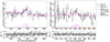 |
Fig. 5. Analysis of the broad emission lines in VIK J2318−31. Top panels: zoomed-in view of the rest-frame CIV (left) and MgII (right) emission lines of VIK J2318−31. The grey line shows the rest-frame spectrum. The best-fit, continuum plus emission lines, is shown as a solid magenta line. In both cases we used two Gaussian components (dashed magenta lines), but in the case of the MgII line we fixed the width and the normalisation of the components to be equal and the relative position of the peaks to 7.2 Å. The Balmer and the iron pseudo-continuum contributions are shown as a dotted blue line and a dashed-dotted orange line, respectively. Bottom panels: residual of the fit divided by the error on the spectrum at each wavelength. Shaded areas indicate ±1,2σ. |
Results of the fit of the CIV and MgII broad emission lines in VIK J2318−31.
As shown in Fig. 5, the CIV line profile can be described by two Gaussian functions, a blueshifted broad component with λcen = 1533.5 Å and σ = 7.7 Å and a narrower component with λcen = 1546.1 Å and σ = 3.6 Å (strictly speaking, this is still a broad emission line, having a full width at half maximum (FWHM) of 1880 km s−1). To compute the total blueshift, we used Δv = c(1549.5 @@@−λhalf)/1549.5 Å (e.g., Coatman et al. 2017), where 1549.5 Å is the rest-frame wavelength of the CIV line, c is the speed of light and λhalf = 1539 ± 2 is the line centroid, that is, the bisector of the cumulative line flux. In the case of VIK J2318−31 we find Δv = 2110 km s−1, which is a relatively large value, but it is still consistent to what is typically measured in high-redshift QSOs (see e.g., Table 1 in Mazzucchelli et al. 2023). The presence of a large CIV blueshift normally indicates that the profile of the line is strongly affected by emission from regions in non-virial motions, that is, with strong outflows (e.g., Baskin & Laor 2005). Interestingly, while RL QSOs present, on average, smaller blueshifts in the CIV with respect to RQ QSOs (see e.g., Richards et al. 2011), the value derived for VIK J2318−31 is the largest currently found in z > 6 RL QSOs (see e.g., Bañados et al. 2021; Belladitta et al. 2022), potentially indicating the presence of important outflows, and, consequently, of feedback (e.g., Maiolino et al. 2012), also for the RL population in the early Universe. At the same time, given the rest-frame equivalent width (REW) of the CIV line (8.8 ± 0.9 Å), the presence of a large blueshift is consistent with the trend of increasing blueshift values for decreasing REW (e.g., Vietri et al. 2018).
Given the asymmetry due to the blueshifted component observed in the CIV line profile of VIK J2318−31, in order to estimate the BH mass we considered the empirical correction derived by Coatman et al. (2017) to the full width at half maximum of the CIV line (Eq. (4) in their paper), which was computed from the comparison of the results obtained with the CIV and the Hα/Hβ emission lines. In this way, the relation used to estimate the BH mass should have a significantly smaller scatter (∼0.2 dex) compared to the un-corrected values. Using the following empirical relation, derived by Vestergaard & Peterson (2006), we computed the mass of the central BH of VIK J2318−31:
where the λL1350 Å luminosity was computed directly from the spectrum continuum. Using this relation, we find MBH = 8.1 ± 5.0 × 10⁸ M⊙, where the statistical errors are comparable to the scatter of the scaling relation: ∼0.2 dex; with the blueshift correction, Coatman et al. (2017), or ∼0.36 dex without this correction, Vestergaard & Peterson (2006).
At the same time, we also used the MgII line in order to compute the SMBH mass. We followed a similar procedure for the analysis of the MgII line and the computation of the related uncertainties, with respect to the CIV line. We considered again two Gaussian components, since the MgII line is composed of a doublet with central wavelengths 2795.5 Å and 2802.7 Å. However, in this case, we used two Gaussian functions with the same width and normalisation and with the relative peak wavelength separation fixed to 7.2 Å. In this way, we still had three free parameters, as in the case of a single Gaussian. We show a zoomed-in view of the MgII together with its best fit in the right panel of Fig. 3. The estimates, and the corresponding errors, obtained from the fit are reported in Table 3. Uncertainties were computed, once again, with Monte Carlo simulations. In order to derive the BH mass of VIK J2318−31 from the MgII line we used the following scaling relation (from Vestergaard & Osmer 2009):
where the λL3000 Å luminosity was computed directly from the spectrum continuum. Using this relation, we find MBH = 4.2 ± 3.0 × 10⁸ M⊙, where the scatter of the relation is ∼0.55 dex.
3.3.2. Bolometric luminosity and Eddington ratio
Having an estimate for the mass of the SMBH in VIK J2318−31, we could then derive how fast the SMBH is accreting. In particular, following the literature, we can compute the λEDD parameter, defined as the ratio between the bolometric luminosity (Lbol), and the Eddington Luminosity LEDD. To estimate Lbol we used the continuum luminosity of VIK J2318−31 derived from its NIR spectrum (L1350 Å = 2.5 ± 0.1 × 1046 erg s−1) and the bolometric corrections computed by Shen et al. (2008) (K = 3.81 ± 1.26). In this way we find: Lbol = K × L1350 Å = 8.4 ± 2.8 × 1046 erg s−1 and λEDD = 0.8 ± 0.6. If we consider the MgII estimate and the continuum at 3000 Å, we obtain: Lbol = 6.6 ± 1.6 × 1046 erg s−1 and λEDD = 1.2 ± 0.8. Interestingly, in both cases, observations suggest that VIK J2318−31 is hosting a highly accreting SMBH, of the order of its Eddington limit.
3.3.3. Accretion disc model
In order to test the presence of possible biases in the BH mass estimate from broad emission lines, we also used another independent method. In particular, we modelled the continuum optical-NIR (UV-optical in the rest frame) emission of VIK J2318−31 with an AD model2 (e.g., Calderone et al. 2013; Ghisellini et al. 2015; Diana et al. 2022). Following the Shakura & Sunyaev (1973; SS) model, we assumed that the optical/UV continuum emission of the active galactic nucleus (AGN) is produced by an optically thick, geometrically thin AD composed of rings that emit as a black body (BB) with different temperatures, where the inner radius of the disc is set to Rin = 3Rs and the outer radius to Rout = 104Rs3. In this model, the free parameters available are the BH mass (MBH), the accretion rate (Ṁ) and the viewing angle (θ). We fixed the latter to θ = 30°, since, as mentioned before, this source is an un-obscured AGN with a jet that is not oriented close to our line of sight. Moreover, we note that we are technically considering a non-rotating SMBH, even though VIK J2318−31 is a RL QSO and therefore expected to be associated with a spinning BHs (e.g., Tchekhovskoy et al. 2010). However, as in similar studies (e.g., Belladitta et al. 2022; Sbarrato et al. 2022), this choice can be justified by the fact that a SS AD with Rin = 3Rs is a good approximation of a rotating BH with spin a = 0.71 (based on the KERRBB model discussed in Li et al. 2005; see e.g., Fig. A2 in Calderone et al. 2013). Under these assumptions, the overall disc luminosity is given by
![$$ \begin{aligned} \mathrm{L}(\nu , {M}_{\rm BH}, \dot{M})\mathrm{d}\nu = \int ^{R_{\rm out}}_{R_{\rm in}} {r B_{\nu }}[{T(r,M_{\rm BH},}\dot{M})]\mathrm{d}\nu \mathrm{d}r, \end{aligned} $$](/articles/aa/full_html/2024/07/aa49369-24/aa49369-24-eq28.gif)
where r is the distance from the centre of the BH and Bν is the Planck BB spectral density at the temperature T. The temperature of the BB depends on the distance from the BH (as T ∝ r−3/4), the mass of the BH (as  ) and the accretion rate (as T ∝ r1/4). In particular, the higher the mass of the BH is, the lower the frequency peak of the spectral energy distribution is.
In order to perform a fit to the model outlined above, we considered the continuum emission from the observed NIR spectrum (GNIRS+X-shooter) described in Sect. 2. In particular, we averaged the NIR spectrum in ranges unaffected by telluric adsorption and without emission lines (see the cyan shaded regions in Fig. 2). As a conservative estimate of the mean flux density errors, we considered the RMS of the spectrum (smoothed to a common 500 km s−1 resolution), by noting that these errors do not significantly impacting the result of the fit, since they have similar values. We report in Table 4 the magnitudes and the corresponding errors obtained. Moreover, in the fit, we also consider the W1 band (mag = 20.71 ± 0.13; in the AB system) from the Wide-field Infrared Survey Explorer (Wright et al. 2010) catalogue (catWISE; Eisenhardt et al. 2020). From the fit to these data points, we obtain  and
and  . Figure 6 shows the best-fit model (solid black line) with the associated 1σ uncertainty (shaded grey area) in the top panel and the corner plot of the parameters derived from the fit in the bottom panel.
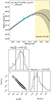 |
Fig. 6. Accretion disc model fit to the optical/NIR emission of VIK J2318−31. Top panel: rest-frame optical-UV luminosities of VIK J2318−31 (cyan points) together with the best-fit SS AD model (solid black line). The shaded blue area represents the model within the 16th and 84th percentiles. The hatched yellow region at ν > 3.3 × 10¹⁵ Hz indicates frequencies higher than the Lyα emission line, which not accessible at high redshift due to the absorption from the IGM. Bottom panels: corner plot with the posterior distributions of the parameters used in the fit. Dashed vertical lines indicate the 16th, 50th and 84th percentiles. |
Both MBH and λEDD derived from the AD model are consistent with the values found through the single epoch estimate. This suggests that the values estimated from the CIV and MgII lines can be considered reliable within the extent of their uncertainty. Given the higher S/N4 of the CIV line (∼10) compared to the MgII one (∼5), we consider  and
and  as the best estimate for the mass and the accretion rate, respectively, of the central BH in VIK J2318−31 (where we also added in quadrature the scatter of the scaling relation used in Eq. (4)).
4. Discussion and conclusions
VIK J2318−31 hosts a ∼8 × 10⁸ M⊙ SMBH accreting close to the Eddington limit. The radio luminosity and spectral shape of this source suggests that the radio emission is powered by young relativistic jets (see also the discussion in Ighina et al. 2022a). Indeed, the compact radio morphology (Zhang et al. 2022) and the presence of a turnover around ∼650 MHz (observed frame) in the radio spectrum are typical signs of young radio jets (see e.g., O’Dea & Saikia 2021). Even though it is not possible to confirm the origin of the turnover in the radio spectrum of VIK J2318−31, due to the lack of information at very low frequencies (≲200 MHz), it seems unlikely to be generated by SSA, since that would require an emitting region orders of magnitude smaller than what is typically found in radio peaked sources (e.g., Orienti & Dallacasa 2008, 2014). At the same time, the shape and the peak frequency derived for VIK J2318−31 are consistent with previous studies on z ≳ 5 RL QSOs (e.g., Shao et al. 2020, 2022).
From the X-ray point of view, the faint and steep (Γ ≳ 1.7) emission observed in VIK J2318−31 suggests that relativistic boosting has only a marginal impact and, therefore, that the jets are oriented away from our line of sight. Interestingly, VIK J2318−31 is the faintest z > 6 RL QSO currently known (Medvedev et al. 2020; Moretti et al. 2021), though the current number of such sources with dedicated X-ray observations is extremely limited.
With respect to other z ≳ 5.7 bright QSOs with a single epoch estimate (either from the CIV or MgII line) from the literature, the properties of the SMBH hosted in VIK J2318−31 are consistent with the observed distributions. In particular, compared to the samples analysed in Shen et al. (2019) and Mazzucchelli et al. (2023), ∼90 individual sources in total, the BH mass derived for VIK J2318−31 falls into the lower end of the distribution (within the lowest ∼10%), while its accretion rate is fully consistent with what is typically found in these high-z systems, that is, an accretion close to the Eddington limit (median value λEdd ∼ 0.7). The agreement between the values obtained for VIK J2318−31 and the rest of the high-z population is likely due to the similar optical selection adopted for their discovery. Indeed, the recent discovery of many faint objects (about two orders of magnitude fainter in the optical compared to VIK J2318−31) at z > 4 with the JWST revealed the presence of a large population of AGN (referred to as ‘little red dots’; see e.g., Matthee et al. 2024; Kocevski et al. 2023) hosting ∼107 − 8 M⊙ SMBHs.
Even though the number of z > 5 QSOs with dedicated NIR spectroscopy and analysis has significantly increased in the last few years (e.g., Mazzucchelli et al. 2023; Lai et al. 2023), only ∼10 of these sources host relativistic jets (i.e., are RL; see Yi et al. 2014; Bañados et al. 2021; Diana et al. 2022; Belladitta et al. 2022, 2023). Therefore, given the small statistics, it is not possible to derive solid conclusions on potential differences between the RL and RQ classes at these very high redshifts. While the mass and the accretion rate found in VIK J2318−31 are similar to the other few high-z SMBHs hosted in RL systems from the literature (again, due to a similar optical selection), this source presents one of the largest blueshifts in the CIV line currently found in this specific QSO class (e.g., Bañados et al. 2021; Belladitta et al. 2022). Given the weakness of the CIV line (REW = 8.8 ± 0.9 Å), the high blueshift value derived for VIK J2318−31 is also consistent with the trend typically found in QSOs. Even though the origin of this relation is not clear yet (see e.g., the discussion in Sun et al. 2018), the faintest CIV lines typically present the largest blueshifts, with sources having REW[CIV] ≲ 15 Å showing blueshifts of up to ∼4000 − 5000 km s−1 (e.g., Ge et al. 2019). Based on the threshold adopted in Diamond-Stanic et al. (2009), VIK J2318−31 is classified as a weak emission line quasar WELQ (i.e., REW[CIV] ≲ 15 Å). Interestingly, recent studies seem to find a larger fraction of WELQs (based on a weak Lyα emission line) hosted in high-z RL systems (e.g., Gloudemans et al. 2022) compared to RQ QSOs at both high (e.g., Bañados et al. 2016) and low redshifts (Diamond-Stanic et al. 2009). The systematic spectroscopic study of these specific high-z RL sources will help us understand the connection between relativistic jets, accretion, and outflows in the early Universe.
The discovery of less massive (e.g., Matthee et al. 2024) and/or faster-accreting (e.g., Wolf et al. 2023) SMBHs at high redshifts can help alleviate the tension between current observations of massive SMBHs hosted in z ∼ 6.5 QSOs and theoretical models that describe their formation as seed BHs (see e.g., Fig. 10 in Onoue et al. 2019). Indeed, the high accretion rate found for VIK J2318−31 could explain the SMBH observed at z = 6.44 as produced by a dense primordial star cluster with a seed mass of ∼104 M⊙ formed at z ∼ 25 and accreting with a radiative efficiency ηd ∼ 0.1. However, the fact that this source is RL could imply that its radiative efficiency is closer to ∼0.3. In this case, an already massive BH (∼5 × 10⁷ M⊙) is needed at z ∼ 25, which cannot be explained even by a direct collapse of primordial gas clouds since this can only happen after the first generation of stars (z ∼ 10 − 15; Smith & Bromm 2019; Woods et al. 2019). However, the very young age of the radio jet suggests that the SMBH accreted with an efficiency ηd ∼ 0.1 for most of its growth and only very recently spun up to produce and launch the relativistic jets. Another potential explanation of the high observed mass is that only a part of the gravitational energy of the accreting gas is heating the disc (e.g., Jolley & Kuncic 2008; Jolley et al. 2009), with the rest amplifying the magnetic field, a necessary component for the launching of relativistic jets (e.g., Blandford & Znajek 1977). Therefore, even though the total efficiency of the accreting process is still η ∼ 0.3, only a fraction (ηd ∼ 0.1; radiative efficiency; e.g., Ghisellini et al. 2013, 2015) is responsible for the disc luminosity and, as a consequence, the Eddington limit. By having a higher Eddington limit to their accretion, SMBHs able to produce relativistic jets can grow faster in this scenario with respect to the canonical model and, potentially, even with respect to the RQ counterparts (see e.g., Fig. 1 in Connor et al. 2024). Finally, another possible way to ease the tension between the high masses observed and the little time available to grow, is the presence of multiple mergers in seed BHs. While, in general, at high redshift we do not expect mergers to be the dominant component in the mass growth of the seed BH population since they are too light to find a merging companion (e.g., Volonteri et al. 2021), from the study of the galaxy kinematics of VIK J2318−31, Neeleman et al. (2021) find that the distribution of the [CII] emission can potentially be disturbed by a recent merger. Even though the results of Neeleman et al. (2021) are based on a low S/N image (∼5), we cannot exclude that a fraction of the mass of the SMBHs hosted by VIK J2318−31 comes from merger activity.
A statistical sample of RL QSOs at high redshifts with multi-wavelength coverage is needed to assess the importance of relativistic jets in the growth of the first seed BHs.
From the observational point of view, a source is defined as RL if the rest-frame flux density ratio S5GHz/S4400Å > 10 (Kellermann et al. 1989).
See https://github.com/FabioRigamonti/pyADfit.git for the code used in this work.
Acknowledgments
We want to thank the anonymous referee for their suggestions to improve the quality of the paper. We want to thank D. Dallacasa for his suggestions and comments regarding the radio properties of the source discussed here. LI, AC and AM acknowledge financial support from the INAF under the project ‘QSO jets in the early Universe’, Ricerca Fondamentale 2022. NHW is supported by an Australian Research Council Future Fellowship (project number FT190100231) funded by the Australian Government. This scientific work makes use of the Murchison Radio-astronomy Observatory, operated by CSIRO. We acknowledge again the Wajarri Yamatji people as the traditional owners of the Observatory site. Support for the operation of the MWA is provided by the Australian Government (NCRIS), under a contract to Curtin University administered by Astronomy Australia Limited. We acknowledge the Pawsey Supercomputing Centre which is supported by the Western Australian and Australian Governments. The Australia Telescope Compact Array is part of the Australia Telescope National Facility (https://ror.org/05qajvd42) which is funded by the Australian Government for operation as a National Facility managed by CSIRO. We acknowledge the Gomeroi people as the Traditional Owners of the Observatory site. We thank the staff of the GMRT who have made these observations possible. The GMRT is run by the National Centre for Radio Astrophysics of the Tata Institute of Fundamental Research. The scientific results reported in this article are based in part on observations made by the Chandra X-ray Observatory. This work was enabled by observations made from the Gemini North telescope, located within the Maunakea Science Reserve and adjacent to the summit of Maunakea. We are grateful for the privilege of observing the Universe from a place that is unique in both its astronomical quality and its cultural significance. Based on observations collected at the European Organisation for Astronomical Research in the Southern Hemisphere under ESO programme 097.B-1070. This research made use of PypeIt, a Python package for semi-automated reduction of astronomical slit-based spectroscopy (Prochaska et al. 2020a,b). This research made use of Astropy, a community-developed core Python package for Astronomy (Astropy Collaboration 2013, 2018).
References
- An, T., & Baan, W. A. 2012, ApJ, 760, 77 [Google Scholar]
- An, T., Mohan, P., Zhang, Y., et al. 2020, Nat. Commun., 11, 143 [Google Scholar]
- Astropy Collaboration (Robitaille, T. P., et al.) 2013, A&A, 558, A33 [NASA ADS] [CrossRef] [EDP Sciences] [Google Scholar]
- Astropy Collaboration (Price-Whelan, A. M., et al.) 2018, AJ, 156, 123 [Google Scholar]
- Bagchi, J., Vivek, M., Vikram, V., et al. 2014, ApJ, 788, 174 [NASA ADS] [CrossRef] [Google Scholar]
- Bañados, E., Venemans, B. P., Decarli, R., et al. 2016, ApJS, 227, 11 [Google Scholar]
- Bañados, E., Mazzucchelli, C., Momjian, E., et al. 2021, ApJ, 909, 80 [CrossRef] [Google Scholar]
- Bañados, E., Schindler, J.-T., Venemans, B. P., et al. 2023, ApJS, 265, 29 [CrossRef] [Google Scholar]
- Banik, N., Tan, J. C., & Monaco, P. 2019, MNRAS, 483, 3592 [NASA ADS] [CrossRef] [Google Scholar]
- Baskin, A., & Laor, A. 2005, MNRAS, 356, 1029 [NASA ADS] [CrossRef] [Google Scholar]
- Belladitta, S., Moretti, A., Caccianiga, A., et al. 2020, A&A, 635, L7 [EDP Sciences] [Google Scholar]
- Belladitta, S., Caccianiga, A., Diana, A., et al. 2022, A&A, 660, A74 [NASA ADS] [CrossRef] [EDP Sciences] [Google Scholar]
- Belladitta, S., Moretti, A., Caccianiga, A., et al. 2023, A&A, 669, A134 [NASA ADS] [CrossRef] [EDP Sciences] [Google Scholar]
- Bentz, M. C., Peterson, B. M., Netzer, H., Pogge, R. W., & Vestergaard, M. 2009, ApJ, 697, 160 [Google Scholar]
- Blandford, R. D., & Znajek, R. L. 1977, MNRAS, 179, 433 [NASA ADS] [CrossRef] [Google Scholar]
- Blandford, R., Meier, D., & Readhead, A. 2019, ARA&A, 57, 467 [NASA ADS] [CrossRef] [Google Scholar]
- Calderone, G., Ghisellini, G., Colpi, M., & Dotti, M. 2013, MNRAS, 431, 210 [NASA ADS] [CrossRef] [Google Scholar]
- Callingham, J. R., Ekers, R. D., Gaensler, B. M., et al. 2017, ApJ, 836, 174 [CrossRef] [Google Scholar]
- Carnall, A. C. 2017, arXiv e-prints [arXiv:1705.05165] [Google Scholar]
- Cash, W. 1979, ApJ, 228, 939 [Google Scholar]
- Clough, S. A., Shephard, M. W., Mlawer, E. J., et al. 2005, J. Quant. Spectr. Rad. Transf., 91, 233 [NASA ADS] [CrossRef] [Google Scholar]
- Coatman, L., Hewett, P. C., Banerji, M., et al. 2017, MNRAS, 465, 2120 [Google Scholar]
- Connor, T., Bañados, E., Cappelluti, N., & Foord, A. 2024, Universe, 10, 227 [CrossRef] [Google Scholar]
- Dallacasa, D., Stanghellini, C., Centonza, M., & Fanti, R. 2000, A&A, 363, 887 [NASA ADS] [Google Scholar]
- Decarli, R., Walter, F., Venemans, B. P., et al. 2018, ApJ, 854, 97 [Google Scholar]
- Devecchi, B., & Volonteri, M. 2009, ApJ, 694, 302 [NASA ADS] [CrossRef] [Google Scholar]
- Diamond-Stanic, A. M., Fan, X., Brandt, W. N., et al. 2009, ApJ, 699, 782 [NASA ADS] [CrossRef] [Google Scholar]
- Diana, A., Caccianiga, A., Ighina, L., et al. 2022, MNRAS, 511, 5436 [NASA ADS] [CrossRef] [Google Scholar]
- Driver, S. P., Hill, D. T., Kelvin, L. S., et al. 2011, MNRAS, 413, 971 [Google Scholar]
- Drouart, G., & Falkendal, T. 2018a, MNRAS, 477, 4981 [NASA ADS] [CrossRef] [Google Scholar]
- Drouart, G., & Falkendal, T. 2018b, Astrophysics Source Code Library [record ascl:1809.015] [Google Scholar]
- Drouart, G., Seymour, N., Galvin, T. J., et al. 2020, PASA, 37, e026 [Google Scholar]
- Duchesne, S. W., Thomson, A. J. M., Pritchard, J., et al. 2023, PASA, 40, e034 [NASA ADS] [CrossRef] [Google Scholar]
- Eisenhardt, P. R. M., Marocco, F., Fowler, J. W., et al. 2020, ApJS, 247, 69 [Google Scholar]
- Elias, J. H., Joyce, R. R., Liang, M., et al. 2006a, in SPIE Conf. Ser., eds. I. S. McLean, & M. Iye, 6269, 62694C [NASA ADS] [Google Scholar]
- Elias, J. H., Rodgers, B., Joyce, R. R., et al. 2006b, in SPIE Conf. Ser., eds. I. S. McLean, & M. Iye, 6269, 626914 [NASA ADS] [Google Scholar]
- Endsley, R., Stark, D. P., Fan, X., et al. 2022, MNRAS, 512, 4248 [CrossRef] [Google Scholar]
- Endsley, R., Stark, D. P., Lyu, J., et al. 2023, MNRAS, 520, 4609 [Google Scholar]
- Farina, E. P., Schindler, J.-T., Walter, F., et al. 2022, ApJ, 941, 106 [NASA ADS] [CrossRef] [Google Scholar]
- Ferrara, A., Salvadori, S., Yue, B., & Schleicher, D. 2014, MNRAS, 443, 2410 [NASA ADS] [CrossRef] [Google Scholar]
- Fitzpatrick, E. L. 1999, PASP, 111, 63 [Google Scholar]
- Freudling, W., Romaniello, M., Bramich, D. M., et al. 2013, A&A, 559, A96 [NASA ADS] [CrossRef] [EDP Sciences] [Google Scholar]
- Fruscione, A., McDowell, J. C., Allen, G. E., et al. 2006, in SPIE Conf. Ser., eds. D. R. Silva, & R. E. Doxsey, 6270, 62701V [Google Scholar]
- Ge, X., Zhao, B.-X., Bian, W.-H., & Frederick, G. R. 2019, AJ, 157, 148 [NASA ADS] [CrossRef] [Google Scholar]
- Ghisellini, G. 2013, Radiative Processes in High Energy Astrophysics (New York: Springer) [Google Scholar]
- Ghisellini, G. 2015, J. High Energy Astrophys., 7, 163 [NASA ADS] [CrossRef] [Google Scholar]
- Ghisellini, G., Haardt, F., Della Ceca, R., Volonteri, M., & Sbarrato, T. 2013, MNRAS, 432, 2818 [NASA ADS] [CrossRef] [Google Scholar]
- Ghisellini, G., Tagliaferri, G., Sbarrato, T., & Gehrels, N. 2015, MNRAS, 450, L34 [NASA ADS] [CrossRef] [Google Scholar]
- Gloudemans, A. J., Duncan, K. J., Röttgering, H. J. A., et al. 2021, A&A, 656, A137 [NASA ADS] [CrossRef] [EDP Sciences] [Google Scholar]
- Gloudemans, A. J., Duncan, K. J., Saxena, A., et al. 2022, A&A, 668, A24 [NASA ADS] [CrossRef] [EDP Sciences] [Google Scholar]
- Gullikson, K., Dodson-Robinson, S., & Kraus, A. 2014, AJ, 148, 53 [NASA ADS] [CrossRef] [Google Scholar]
- Gürkan, G., Prandoni, I., O’Brien, A., et al. 2022, MNRAS, 512, 6104 [CrossRef] [Google Scholar]
- Hale, C. L., McConnell, D., Thomson, A. J. M., et al. 2021, PASA, 38 [CrossRef] [Google Scholar]
- HI4PI Collaboration (Ben Bekhti, N., et al.) 2016, A&A, 594, A116 [NASA ADS] [CrossRef] [EDP Sciences] [Google Scholar]
- Hurley-Walker, N., Callingham, J. R., Hancock, P. J., et al. 2017, MNRAS, 464, 1146 [Google Scholar]
- Ighina, L., Caccianiga, A., Moretti, A., et al. 2019, MNRAS, 489, 2732 [NASA ADS] [CrossRef] [Google Scholar]
- Ighina, L., Belladitta, S., Caccianiga, A., et al. 2021, A&A, 647, L11 [NASA ADS] [CrossRef] [EDP Sciences] [Google Scholar]
- Ighina, L., Leung, J. K., Broderick, J. W., et al. 2022a, A&A, 663, A73 [NASA ADS] [CrossRef] [EDP Sciences] [Google Scholar]
- Ighina, L., Moretti, A., Tavecchio, F., et al. 2022b, A&A, 659, A93 [NASA ADS] [CrossRef] [EDP Sciences] [Google Scholar]
- Ighina, L., Caccianiga, A., Moretti, A., et al. 2023, MNRAS, 519, 2060 [Google Scholar]
- Jolley, E. J. D., & Kuncic, Z. 2008, MNRAS, 386, 989 [NASA ADS] [CrossRef] [Google Scholar]
- Jolley, E. J. D., Kuncic, Z., Bicknell, G. V., & Wagner, S. 2009, MNRAS, 400, 1521 [NASA ADS] [CrossRef] [Google Scholar]
- Kale, R., & Ishwara-Chandra, C. H. 2021, Exp. Astron., 51, 95 [NASA ADS] [CrossRef] [Google Scholar]
- Kaspi, S., Smith, P. S., Netzer, H., et al. 2000, ApJ, 533, 631 [Google Scholar]
- Keim, M. A., Callingham, J. R., & Röttgering, H. J. A. 2019, A&A, 628, A56 [NASA ADS] [CrossRef] [EDP Sciences] [Google Scholar]
- Kellermann, K. I., & Pauliny-Toth, I. I. K. 1981, ARA&A, 19, 373 [NASA ADS] [CrossRef] [Google Scholar]
- Kellermann, K. I., Sramek, R., Schmidt, M., Shaffer, D. B., & Green, R. 1989, AJ, 98, 1195 [Google Scholar]
- Kocevski, D. D., Onoue, M., Inayoshi, K., et al. 2023, ApJ, 954, L4 [NASA ADS] [CrossRef] [Google Scholar]
- Lai, S., Onken, C. A., Wolf, C., et al. 2023, MNRAS, 526, 3230 [NASA ADS] [CrossRef] [Google Scholar]
- Lambrides, E., Chiaberge, M., Long, A. S., et al. 2024, ApJ, 961, L25 [NASA ADS] [CrossRef] [Google Scholar]
- Li, L.-X., Zimmerman, E. R., Narayan, R., & McClintock, J. E. 2005, ApJS, 157, 335 [NASA ADS] [CrossRef] [Google Scholar]
- Lusso, E., & Risaliti, G. 2016, ApJ, 819, 154 [Google Scholar]
- Mahato, M., Dabhade, P., Saikia, D. J., et al. 2022, A&A, 660, A59 [NASA ADS] [CrossRef] [EDP Sciences] [Google Scholar]
- Maio, U., Borgani, S., Ciardi, B., & Petkova, M. 2019, PASA, 36, e020 [CrossRef] [Google Scholar]
- Maiolino, R., Gallerani, S., Neri, R., et al. 2012, MNRAS, 425, L66 [Google Scholar]
- Matthee, J., Naidu, R. P., Brammer, G., et al. 2024, ApJ, 963, 129 [NASA ADS] [CrossRef] [Google Scholar]
- Mazzucchelli, C., Bañados, E., Venemans, B. P., et al. 2017, ApJ, 849, 91 [Google Scholar]
- Mazzucchelli, C., Bischetti, M., D’Odorico, V., et al. 2023, A&A, 676, A71 [NASA ADS] [CrossRef] [EDP Sciences] [Google Scholar]
- McConnell, D., Hale, C. L., Lenc, E., et al. 2020, PASA, 37, e048 [Google Scholar]
- McGreer, I. D., Becker, R. H., Helfand, D. J., & White, R. L. 2006, ApJ, 652, 157 [Google Scholar]
- McMullin, J. P., Waters, B., Schiebel, D., Young, W., & Golap, K. 2007, in Astronomical Data Analysis Software and Systems XVI, eds. R. A. Shaw, F. Hill, & D. J. Bell, ASP Conf. Ser., 376, 127 [Google Scholar]
- Medvedev, P., Sazonov, S., Gilfanov, M., et al. 2020, MNRAS, 497, 1842 [Google Scholar]
- Moretti, A., Ghisellini, G., Caccianiga, A., et al. 2021, ApJ, 920, 15 [NASA ADS] [CrossRef] [Google Scholar]
- Nanni, R., Vignali, C., Gilli, R., Moretti, A., & Brandt, W. N. 2017, A&A, 603, A128 [NASA ADS] [CrossRef] [EDP Sciences] [Google Scholar]
- Neeleman, M., Novak, M., Venemans, B. P., et al. 2021, ApJ, 911, 141 [NASA ADS] [CrossRef] [Google Scholar]
- O’Dea, C. P., & Saikia, D. J. 2021, A&A Rev., 29, 3 [CrossRef] [Google Scholar]
- Oh, S. P., & Haiman, Z. 2002, ApJ, 569, 558 [NASA ADS] [CrossRef] [Google Scholar]
- Onoue, M., Kashikawa, N., Matsuoka, Y., et al. 2019, ApJ, 880, 77 [Google Scholar]
- Orienti, M., & Dallacasa, D. 2008, A&A, 477, 807 [NASA ADS] [CrossRef] [EDP Sciences] [Google Scholar]
- Orienti, M., & Dallacasa, D. 2014, MNRAS, 438, 463 [NASA ADS] [CrossRef] [Google Scholar]
- Pacholczyk, A. G. 1970, Radio Astrophysics. Nonthermal Processes in Galactic and Extragalactic Sources (San Francisco: Freeman) [Google Scholar]
- Pacucci, F., Natarajan, P., Volonteri, M., Cappelluti, N., & Urry, C. M. 2017, ApJ, 850, L42 [NASA ADS] [CrossRef] [Google Scholar]
- Padovani, P. 2017, Nat. Astron., 1, 0194 [Google Scholar]
- Paliya, V. S., Domínguez, A., Cabello, C., et al. 2020, ApJ, 903, L8 [NASA ADS] [CrossRef] [Google Scholar]
- Pezzulli, E., Valiante, R., & Schneider, R. 2016, MNRAS, 458, 3047 [NASA ADS] [CrossRef] [Google Scholar]
- Piconcelli, E., Jimenez-Bailón, E., Guainazzi, M., et al. 2005, A&A, 432, 15 [NASA ADS] [CrossRef] [EDP Sciences] [Google Scholar]
- Prochaska, J., Hennawi, J., Westfall, K., et al. 2020a, J. Open Source Softw., 5, 2308 [NASA ADS] [CrossRef] [Google Scholar]
- Prochaska, J. X., Hennawi, J., Cooke, R., et al. 2020b, https://doi.org/10.5281/zenodo.3743493 [Google Scholar]
- Quici, B., Hurley-Walker, N., Seymour, N., et al. 2021, PASA, 38, e008 [CrossRef] [Google Scholar]
- Reddy, S. H., Kudale, S., Gokhale, U., et al. 2017, J. Astron. Instrum., 6, 1641011 [CrossRef] [Google Scholar]
- Reynolds, J. 1994, ATNF Technical Memos, AT/39.3/040 [Google Scholar]
- Richards, G. T., Kruczek, N. E., Gallagher, S. C., et al. 2011, AJ, 141, 167 [Google Scholar]
- Ross, K., Reynolds, C., Seymour, N., et al. 2023, PASA, 40, e005 [NASA ADS] [CrossRef] [Google Scholar]
- Sakurai, Y., Yoshida, N., Fujii, M. S., & Hirano, S. 2017, MNRAS, 472, 1677 [NASA ADS] [CrossRef] [Google Scholar]
- Salvestrini, F., Risaliti, G., Bisogni, S., Lusso, E., & Vignali, C. 2019, A&A, 631, A120 [NASA ADS] [CrossRef] [EDP Sciences] [Google Scholar]
- Sault, R. J., Teuben, P. J., & Wright, M. C. H. 1995, in Astronomical Data Analysis Software and Systems IV, eds. R. A. Shaw, H. E. Payne, & J. J. E. Hayes, ASP Conf. Ser., 77, 433 [Google Scholar]
- Sbarrato, T., Ghisellini, G., Tagliaferri, G., et al. 2022, A&A, 663, A147 [NASA ADS] [CrossRef] [EDP Sciences] [Google Scholar]
- Schlafly, E. F., & Finkbeiner, D. P. 2011, ApJ, 737, 103 [Google Scholar]
- Shakura, N. I., & Sunyaev, R. A. 1973, A&A, 24, 337 [NASA ADS] [Google Scholar]
- Shao, Y., Wagg, J., Wang, R., et al. 2020, A&A, 641, A85 [NASA ADS] [CrossRef] [EDP Sciences] [Google Scholar]
- Shao, Y., Wagg, J., Wang, R., et al. 2022, A&A, 659, A159 [NASA ADS] [CrossRef] [EDP Sciences] [Google Scholar]
- Shen, Y., Greene, J. E., Strauss, M. A., Richards, G. T., & Schneider, D. P. 2008, ApJ, 680, 169 [Google Scholar]
- Shen, Y., Wu, J., Jiang, L., et al. 2019, ApJ, 873, 35 [Google Scholar]
- Shen, X., Hopkins, P. F., Faucher-Giguère, C.-A., et al. 2020, MNRAS, 495, 3252 [Google Scholar]
- Shimwell, T. W., Röttgering, H. J. A., Best, P. N., et al. 2017, A&A, 598, A104 [NASA ADS] [CrossRef] [EDP Sciences] [Google Scholar]
- Shimwell, T. W., Tasse, C., Hardcastle, M. J., et al. 2019, A&A, 622, A1 [NASA ADS] [CrossRef] [EDP Sciences] [Google Scholar]
- Shimwell, T. W., Hardcastle, M. J., Tasse, C., et al. 2022, A&A, 659, A1 [NASA ADS] [CrossRef] [EDP Sciences] [Google Scholar]
- Smith, A., & Bromm, V. 2019, Contemp. Phys., 60, 111 [NASA ADS] [CrossRef] [Google Scholar]
- Spingola, C., Dallacasa, D., Belladitta, S., et al. 2020, A&A, 643, L12 [EDP Sciences] [Google Scholar]
- Sun, M., Xue, Y., Richards, G. T., et al. 2018, ApJ, 854, 128 [NASA ADS] [CrossRef] [Google Scholar]
- Takeo, E., Inayoshi, K., Ohsuga, K., Takahashi, H. R., & Mineshige, S. 2019, MNRAS, 488, 2689 [NASA ADS] [CrossRef] [Google Scholar]
- Tchekhovskoy, A., Narayan, R., & McKinney, J. C. 2010, ApJ, 711, 50 [NASA ADS] [CrossRef] [Google Scholar]
- Thorne, K. S. 1974, ApJ, 191, 507 [Google Scholar]
- Tingay, S. J., Goeke, R., Bowman, J. D., et al. 2013, PASA, 30, e007 [Google Scholar]
- Urry, C. M., & Padovani, P. 1995, PASP, 107, 803 [NASA ADS] [CrossRef] [Google Scholar]
- Venemans, B. P., Walter, F., Neeleman, M., et al. 2020, ApJ, 904, 130 [Google Scholar]
- Vernet, J., Dekker, H., D’Odorico, S., et al. 2011, A&A, 536, A105 [NASA ADS] [CrossRef] [EDP Sciences] [Google Scholar]
- Vestergaard, M., & Osmer, P. S. 2009, ApJ, 699, 800 [Google Scholar]
- Vestergaard, M., & Peterson, B. M. 2006, ApJ, 641, 689 [Google Scholar]
- Vestergaard, M., & Wilkes, B. J. 2001, ApJS, 134, 1 [Google Scholar]
- Vietri, G., Piconcelli, E., Bischetti, M., et al. 2018, A&A, 617, A81 [NASA ADS] [CrossRef] [EDP Sciences] [Google Scholar]
- Vignali, C., Brandt, W. N., Schneider, D. P., & Kaspi, S. 2005, AJ, 129, 2519 [NASA ADS] [CrossRef] [Google Scholar]
- Vito, F., Brandt, W. N., Bauer, F. E., et al. 2019, A&A, 630, A118 [NASA ADS] [CrossRef] [EDP Sciences] [Google Scholar]
- Volonteri, M., Habouzit, M., & Colpi, M. 2021, Nat. Rev. Phys., 3, 732 [NASA ADS] [CrossRef] [Google Scholar]
- Wayth, R. B., Lenc, E., Bell, M. E., et al. 2015, PASA, 32, e025 [Google Scholar]
- Willott, C. J., Delorme, P., Reylé, C., et al. 2010, AJ, 139, 906 [Google Scholar]
- Wilson, W. E., Ferris, R. H., Axtens, P., et al. 2011, MNRAS, 416, 832 [Google Scholar]
- Wolf, J., Nandra, K., Salvato, M., et al. 2023, A&A, 669, A127 [NASA ADS] [CrossRef] [EDP Sciences] [Google Scholar]
- Woods, T. E., Alexandroff, R., Ellison, S., et al. 2019, Canadian Long Range Plan for Astronomy and Astrophysics White Papers, 2020, 34 [Google Scholar]
- Wright, E. L., Eisenhardt, P. R. M., Mainzer, A. K., et al. 2010, AJ, 140, 1868 [Google Scholar]
- Yi, W.-M., Wang, F., Wu, X.-B., et al. 2014, ApJ, 795, L29 [Google Scholar]
- Zhang, Y., An, T., Wang, A., et al. 2022, A&A, 662, L2 [NASA ADS] [CrossRef] [EDP Sciences] [Google Scholar]
Appendix A: Radio Images from MWA, uGMRT, and ATCA
In this section we report the radio images obtained with the MWA (Fig. A.1), the uGMRT (Fig. A.2) and the ATCA (Fig. A.3) telescopes of both epochs. A description of the reduction process is reported in Sect. 2.
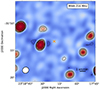 |
Fig. A.1. Cutout around the optical position of VIK J2318−31 (orange cross) of the MWA observations of the G23 field. Contours start at ±3 × RMS and increase by a factor of |

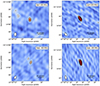 |
Fig. A.2. uGMRT observation of VIK J2318−31 at 400 (left) and 650 MHz (right) at the two different epochs: April 2022 (top) and September 2022 (bottom). Contours start at ±3×RMS and increase by a factor of |

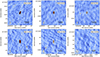 |
Fig. A.3. ATCA observation of VIK J2318−31 at 2.1, 5.5 and 9.0 GHz (from left to right) at the two different epochs: April 2022 (top) and September 2022 (bottom). Contours start at ±3×RMS and increase by a factor of |

All Tables
Best-fit values obtained from the fit of the X-ray spectrum of VIK J2318−31 assuming a simple power law with Galactic absorption (NH = 1.13 × 1020 cm−2; HI4PI Collaboration 2016).
Best-fit flux densities obtained from a Gaussian fit to the radio images of VIK J2318–31 together with the synthesised beam size, position angle (PA), and RMS of each observation.
All Figures
|
Fig. 1. X-ray observations of VIK J2318−31. Left: X-ray image of VIK J2318−31 from a 70 ks Chandra observation. The extraction region for the target and background spectra are reported as a solid green circle and a dotted blue annulus. Right: X-ray spectrum of VIK J2318−31. The best-fit power law spectra obtained using the cstat statistics are reported as a solid blue line (with Γ as a free parameter) and as a dashed-dotted red line (with Γ fixed). The corresponding best-fit values are reported in Table 1. |
| In the text | |
|
Fig. 2. NIR spectrum of VIK J2318−31 obtained from GNIRS+X-shooter observations (black continuum line). The spectrum was re-binned to a resolution of 250 km s−1. The dotted red line indicates the error on the spectrum. The regions affected by strong telluric absorption have been masked. The cyan shaded areas indicate the wavelength regions used to derive the photometric points (cyan circles) used for the accretion model fit. The dashed orange lines indicate the expected wavelength of the brightest emission lines present in the observed spectrum. |
| In the text | |
|
Fig. 3. Rest-frame spectral energy distribution, from the radio to the X-ray band, of VIK J2318−31. Radio data are reported as green squares together with the best-fit curved radio spectrum derived (dashed black line); optical and IR data from the literature are reported as brown inverted triangles, while the photometric points used for the AD model are reported as cyan circles; the X-ray Chandra data are reported as red diamonds together with the expected X-ray emission from the LX−L2500 Å relation derived in Lusso & Risaliti (2016) (assuming Γ = 2; blue shaded region). The shaded yellow area represents the range of optical frequencies where the Lyα absorption from the intergalactic medium takes place. |
| In the text | |
|
Fig. 4. Radio spectrum of VIK J2318−31. Data already presented in Ighina et al. (2022a) are shown as grey pentagons, while new observations are reported as blue squares (April epoch) and orange circles (September epoch). The purple upper-limit is the estimate derived from the new MWA-MIDAS image. The dashed black line shows the best-fit curved spectrum described in the text. The shaded grey area encloses the curves obtained by varying the best-fit parameters by ±1σ. The dashed line shows the best-fit double power law, while the dotted lines are the best-fit single power law describing the data above and below 1.4 GHz in the observed frame. |
| In the text | |
|
Fig. 5. Analysis of the broad emission lines in VIK J2318−31. Top panels: zoomed-in view of the rest-frame CIV (left) and MgII (right) emission lines of VIK J2318−31. The grey line shows the rest-frame spectrum. The best-fit, continuum plus emission lines, is shown as a solid magenta line. In both cases we used two Gaussian components (dashed magenta lines), but in the case of the MgII line we fixed the width and the normalisation of the components to be equal and the relative position of the peaks to 7.2 Å. The Balmer and the iron pseudo-continuum contributions are shown as a dotted blue line and a dashed-dotted orange line, respectively. Bottom panels: residual of the fit divided by the error on the spectrum at each wavelength. Shaded areas indicate ±1,2σ. |
| In the text | |
|
Fig. 6. Accretion disc model fit to the optical/NIR emission of VIK J2318−31. Top panel: rest-frame optical-UV luminosities of VIK J2318−31 (cyan points) together with the best-fit SS AD model (solid black line). The shaded blue area represents the model within the 16th and 84th percentiles. The hatched yellow region at ν > 3.3 × 10¹⁵ Hz indicates frequencies higher than the Lyα emission line, which not accessible at high redshift due to the absorption from the IGM. Bottom panels: corner plot with the posterior distributions of the parameters used in the fit. Dashed vertical lines indicate the 16th, 50th and 84th percentiles. |
| In the text | |
|
Fig. A.1. Cutout around the optical position of VIK J2318−31 (orange cross) of the MWA observations of the G23 field. Contours start at ±3 × RMS and increase by a factor of |
| In the text | |
|
Fig. A.2. uGMRT observation of VIK J2318−31 at 400 (left) and 650 MHz (right) at the two different epochs: April 2022 (top) and September 2022 (bottom). Contours start at ±3×RMS and increase by a factor of |
| In the text | |
|
Fig. A.3. ATCA observation of VIK J2318−31 at 2.1, 5.5 and 9.0 GHz (from left to right) at the two different epochs: April 2022 (top) and September 2022 (bottom). Contours start at ±3×RMS and increase by a factor of |
| In the text | |
Current usage metrics show cumulative count of Article Views (full-text article views including HTML views, PDF and ePub downloads, according to the available data) and Abstracts Views on Vision4Press platform.
Data correspond to usage on the plateform after 2015. The current usage metrics is available 48-96 hours after online publication and is updated daily on week days.
Initial download of the metrics may take a while.