| Issue |
A&A
Volume 684, April 2024
|
|
|---|---|---|
| Article Number | A57 | |
| Number of page(s) | 17 | |
| Section | Cosmology (including clusters of galaxies) | |
| DOI | https://doi.org/10.1051/0004-6361/202348640 | |
| Published online | 04 April 2024 | |
Galaxy clustering multi-scale emulation
Aix-Marseille Univ., CNRS/IN2P3, CPPM, Marseille, France
e-mail: This email address is being protected from spambots. You need JavaScript enabled to view it.
Received:
16
November 2023
Accepted:
23
December 2023
Abstract
Simulation-based inference has seen increasing interest in the past few years as a promising approach to modelling the non-linear scales of galaxy clustering. The common approach, using the Gaussian process, is to train an emulator over the cosmological and galaxy–halo connection parameters independently for every scale. We present a new Gaussian process model that allows the user to extend the input parameter space dimensions and to use a non-diagonal noise covariance matrix. We use our new framework to simultaneously emulate every scale of the non-linear clustering of galaxies in redshift space from the ABACUSSUMMITN-body simulations at redshift z = 0.2. The model includes nine cosmological parameters, five halo occupation distribution (HOD) parameters, and one scale dimension. Accounting for the limited resolution of the simulations, we train our emulator on scales from 0.3 h−1 Mpc to 60 h−1 Mpc and compare its performance with the standard approach of building one independent emulator for each scale. The new model yields more accurate and precise constraints on cosmological parameters compared to the standard approach. As our new model is able to interpolate over the scale space, we are also able to account for the Alcock-Paczynski distortion effect, leading to more accurate constraints on the cosmological parameters.
Key words: galaxies: general / large-scale structure of Universe
© The Authors 2024
 Open Access article, published by EDP Sciences, under the terms of the Creative Commons Attribution License (https://creativecommons.org/licenses/by/4.0), which permits unrestricted use, distribution, and reproduction in any medium, provided the original work is properly cited.
This article is published in open access under the Subscribe to Open model. This email address is being protected from spambots. You need JavaScript enabled to view it. to support open access publication.
1. Introduction
Galaxies are one of the best tracers of the underlying dark matter distribution in our Universe as a function of time. Spectroscopic galaxy surveys have become a powerful probe of the physical laws governing the formation of the large-scale structures because they provide precise spatial information for millions of galaxies over large volumes. Surveys such as the 2dFGRS (Dawson et al. 2013), 6dFGS (Kobayashi et al. 2020), WiggleZ (du Mas des Bourboux et al. 2020), VIPERS (Hadzhiyska et al. 2021), Sloan Digital Sky Survey (SDSS), BOSS, and eBOSS (Garrison et al. 2021; Blanton et al. 2017; Dawson et al. 2016; de Mattia et al. 2021) have proven (and continue) to be strong tools for understanding the accelerated expansion of our Universe and for testing models of dark energy or modified theories of gravity (Yoo & Seljak 2015; Zhai et al. 2023; Jones et al. 2004; Howlett et al. 2015).
The analysis of spectroscopic galaxy surveys consists in the measurement and modelling of two main physical features present in the two-point function of the density field: the baryon acoustic oscillations (BAOs) and the redshift space distortions (RSDs). While BAOs can be well modelled by linear theory, because they manifest as correlations at large linear scales (around 100 h−1 Mpc), RSDs are more challenging because there is valuable information on small, mildly non-linear scales (below a few tens of h−1 Mpc), which are therefore harder to model accurately. The latest measurements of BAOs and RSDs from SDSS have put the tightest constraints on the growth history to date (Alam et al. 2017, 2021; Saatci 2011; Huterer 2023; Bautista et al. 2021; Guzzo et al. 2014; DeRose et al. 2019; Taruya et al. 2010; Hou et al. 2023; Pajer & Zaldarriaga 2013; Eisenstein et al. 2011). Ongoing and future galaxy surveys such as Euclid (Maksimova et al. 2021; Euclid Collaboration 2022) and the Dark Energy Spectroscopic Instrument (DESI, DESI Collaboration 2016; Drinkwater et al. 2010) span deeper and wider fields of view and will measure tens of millions of galaxies. Such samples of galaxies will significantly reduce statistical uncertainties in the two-point functions, requiring higher precision clustering models to derive unbiased cosmological constraints.
Standard perturbative theories attempt to model mildly non-linear scales analytically (Villaescusa-Navarro et al. 2020; Ross et al. 2015; Carlson et al. 2013; Weinberg et al. 2013). Even more modern approaches (including loop corrections), such as the effective field theory of large-scale structure (EFToLSS, Peebles & Hauser 1974; Carrasco et al. 2014), try to push the model validity to smaller scales, but ultimately such perturbative approaches are limited as the density perturbations on small scales become too large, especially at low redshifts.
An alternative to perturbation theory is to build a simulation-based model to extract information from the small-scale clustering. A recent approach consists in running several N-body simulations for different cosmological models, computing the summary statistics for each, and using them to predict the clustering for a new set of cosmological parameters. This process is commonly referred to as emulation. Brute iterative solving of dynamical equations in N-body simulations provide the high-fidelity description of the non-linear clustering of matter, although they are computationally expensive to produce. In recent years, several suites of N-body simulations have been produced for this purpose (DESI Collaboration 2022; Wang et al. 2014; Moon et al. 2023). Several emulators have been developed (Kobayashi et al. 2022) and some of these have been applied to real data to extract cosmological parameters from real data (Kwan et al. 2023; Chapman et al. 2022).
Any statistics derived from the properties of dark-matter tracers suffer from cosmic variance. This effect decreases as the volume of the simulation increases, but ultimately every measured observable comes with its error budget. An emulator should therefore consider the uncertainty of the training set along with the uncertainty of the predictions. A popular emulation algorithm used in previous works for galaxy clustering (Yuan et al. 2022b; Planck Collaboration VI 2020; Landy & Szalay 1993) is the Gaussian process (GP). This Bayesian machine learning method with physical interpretation not only provides a prediction for the model but also an associated uncertainty. However, it is well known that GP models scale poorly with the number of training points N as they require the construction and inversion of an N × N matrix (N is the number of training samples) many times during the training phase. Each of these operations costs O(N2) memory and O(N3) time. As a consequence, the dimension of the input space is often restricted to the cosmology and galaxy-halo connection parameters. In particular, the standard approach of the previous works is to construct an independent emulator for each separation or Fourier mode, ignoring the well-known correlations between scales. In the present work, we propose a new Gaussian process model, allowing us to extend the input parameter space, and therefore to interpolate or extrapolate over a wider range of parameters, such as scales, redshift bins, selection effects, and so on. As a proof of concept, we built an emulator for the two-point correlation function from a redshift z = 0.2 snapshot of the ABACUSSUMMIT suite (Moon et al. 2023), and extended the input parameter space to include the different separation scales. We implemented our new framework on a Graphics Processing Unit (GPU) with the JAX library.
This paper is organised as follows. In Sect. 2, we present the ABACUSSUMMITN-body simulations, the galaxy–halo connection, and the observable. In Sect. 3, we describe the GP framework along with our new model. In Sect. 4, we validate our emulator performance by comparison to a standard model. Finally, in Sect. 5, we explore the constraining power of our model.
2. Emulating clustering from N-body simulations
In this section, we describe the suite of N-body simulations used in this work. As these are dark-matter only, we use a halo occupation distribution (HOD) to populate galaxies. We then discuss the summary statistics we use to evaluate the performance of our emulation technique.
2.1. The ABACUSSUMMIT suite of simulations
ABACUSSUMMIT (Moon et al. 2023) is a suite of N-body simulations run with the Abacus N-body code (Gil-Marín et al. 2020) on the Summit supercomputer of the Oak Ridge Leadership Computing Facility. These simulations were designed to match the requirement of the Dark Energy Spectroscopic Survey (DESI). ABACUSSUMMIT is composed of hundreds of periodic cubic boxes evolved in comoving coordinates to different epochs from redshift z = 8.0 to z = 0.1. The base simulations consist of 69123 particles of mass 2 × 10⁹h−1M⊙ in a 2 h−1Gpc)3 volume, yielding to a resolution of about 0.3 h−1 Mpc. The suite provides halo catalogues formed by identifying groups of particles, built using the specialised spherical-overdensity-based halo finder COMPASO (see Hou et al. 2021 for more details).
ABACUSSUMMIT spans several cosmological models sampled around the best-fit ΛCDM model to Planck 2018 data (Colless et al. 2003) with nine different parameters θΩ = {ωcdm, ωb, σ8, w0, wa, h, ns, Nur, αs}: the dark matter density ωcdm, the baryon density ωb, the clustering amplitude σ8, the dark energy equation of state w(a)=w0 + wa(1 − a), the Hubble constant h, the spectral tilt ns, the density of massless relics Nur, and the running of the spectral tilt αs. A flat curvature is assumed for every cosmology.
Figure 1 shows the sampling over the nine-dimensional space of 88 cosmologies (in blue) used to train the emulator, and 6 cosmologies (in orange) used as a test set, all with the base resolution. The test set includes the centre of the hypercube: the Planck 2018 ΛCDM cosmology with 60 meV neutrinos, the same cosmology with massless neutrinos, four secondary cosmologies with low ωcdm choice based on WMAP7, a wCDM choice, a high Nur choice, and a low σ8 choice. The training set provides a wider coverage of the parameter space. In the following, we use XΩ to refer to the 88 × 9 matrix containing the cosmological parameters of the training set.
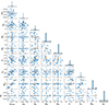 |
Fig. 1. Sampling over the nine-dimensional cosmological space around Planck 2018 ΛCDM. The 88 cosmologies used to train the emulator are shown in blue, while the 6 cosmologies used as a test set are shown in orange. The dark matter density is denoted ωcdm, the baryon density ωb, the clustering amplitude σ8, the dark energy equation of state w(a)=w0 + wa(1 − a), the Hubble constant h, the spectral tilt ns, the density of massless relics Nur, and the running of the spectral tilt αs (Moon et al. 2023). |
All simulations were run with the same initial conditions, and so changes in the measured clustering are only due to changes in cosmology. To test the cosmic variance, ABACUSSUMMIT also provides another set of 25 realisations with the same cosmology and different initial conditions and an additional set of 1400 smaller (500 h−1 Mpc)3 boxes with the same cosmology and mass resolution, but different phases. The small boxes are used to compute sample covariance matrices of our data vectors. All those simulations were run with the base Planck 2018 cosmology. While snapshots are available for several redshifts, we only use snapshots at redshift z = 0.2 throughout this work1.
2.2. Halo occupation distribution model
We use the HOD framework (Zheng et al. 2007) to assign galaxies to dark-matter halos of the simulations. This framework assumes that the number of galaxies N in a given dark matter halo follows a probabilistic distribution P(N|Ωh), where Ωh can be a set of halo properties. In this work, we assume a standard vanilla HOD, where this distribution only depends on the halo’s mass Ωh = M. Moreover, the occupation is decomposed into the contribution of central and satellite galaxies ⟨N(M)⟩ = ⟨Ncen(M)⟩ + ⟨Nsat(M)⟩. The number of central galaxy occupation follows a Bernoulli distribution, while the satellite galaxy occupation follows Poisson distribution. The mean of these distributions are defined as:
 (1)
(1)
![Mathematical equation: $$ \begin{aligned} \langle N_{\rm sat} \rangle&= \left[ \frac{M - \kappa M_{\rm cut}}{M_1} \right]^{\alpha }\langle N_{\rm cen} \rangle , \end{aligned} $$](/articles/aa/full_html/2024/04/aa48640-23/aa48640-23-eq2.gif) (2)
(2)
where erfc(x) is the complimentary error function, θhod = {Mcut, σ, κ, M1, α} are the HOD parameters, Mcut is the minimum mass to host a central galaxy, σ is the width of the cutoff profile (i.e the steepness of the transition 0–1 in the number of central galaxies), κMcut is the minimum mass to host a satellite galaxy, M1 the typical mass to host one satellite galaxy, and α is the power-law index of the satellite occupation.
We used the ABACUSHOD implementation (Zhai et al. 2017), where for each halo, if a random number – drawn from a normal distribution between 0 and 1 – is smaller than ⟨Ncen⟩, a central galaxy is assigned to the centre of mass of the halo with the same velocity. Satellite galaxies do not assume a fixed distribution profile such as the Navarro-Frenk-White profile (Neveux et al. 2020), but rather follow the distribution of the dark matter particles. Specifically, each particle inside a halo has the same probability of hosting a satellite galaxy p = ⟨Nsat⟩/Np with Np being the number of particles in a given halo. For every particle, a random number between 0 and 1 is drawn; if it is smaller than p, a galaxy is assigned to its position with the same velocity. The ABACUSUTILS package implements this halo occupation scheme and is publicly available2.
To build our training set, we populated each of the 88 boxes with 600 HODs selected using a latin hypercube sampling, resulting in 52 800 different clustering measurements. For the test set, we used a different set of 20 HODs to populate the six test cosmologies. We chose the parameter ranges according to the bright galaxy sample of the DESI one percent survey (Rasmussen & Williams 2006). In the following, we use XHOD to refer to the 600 × 5 matrix containing the HOD parameters of the training set. We note that using the same HOD sampling for every cosmology results in a grid-structured parameter space XΩ ⊗ XHOD, where ⊗ is the Kronecker product. This peculiar data structure is useful when building the emulator, which we demonstrate in Sect. 3. Figure 2 illustrates the different forms that the number of galaxies as a function of halo mass takes for the wide range of HOD parametrisation that we use. The black lines show the mean HOD configuration for ⟨Ncen(M)⟩, ⟨Nsat(M)⟩, and ⟨Ntot(M)⟩. Table 1 summarises the sampling range of every cosmological and HOD parameter.
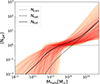 |
Fig. 2. Different forms that take the total occupation of the galaxy for the 600 HOD parametrisation used. The black lines show the mean HOD configuration for ⟨Ncen(M)⟩, ⟨Nsat(M)⟩, and ⟨Ntot(M)⟩. |
Cosmological and HOD parameter names and ranges sampled to build the emulator training and testing sets.
2.3. Observable of interest: The correlation function
To capture the cosmological information in the small-scale clustering of galaxies, we use the standard statistic referred to as the two-point correlation function (2PCF) as an observable. The 2PCF is defined as ξ(r1 − r2)=⟨δg(r1)δg(r2)⟩, where δg(r) is the over-density of galaxies at position r. The 2PCF is measured in a catalogue by counting the pairs of galaxies with the well-known Landy-Szalay estimator (Laureijs et al. 2011):
 (3)
(3)
where DD, RR, DR, and RD are the normalised pair counts of data–data, random–random, data–random, and random–data catalogues. The random catalogue is used to define the window function of the survey. Because each galaxy has its own peculiar velocity on top of the Hubble flow, the measured positions of galaxies along the line of sight (LoS) are modified by the so-called redshift-space distortions (RSDs) as:
 (4)
(4)
where d and ds are the true and distorted radial position, v∥ is the peculiar velocity along the LoS, and H(z) is the Hubble parameter at that redshift. We note that, because we are using snapshots of N-body instead of light cones, the redshift evolution is not simulated and here z has the same value of 0.2 for all galaxies.
Because of RSD, the 2PCF loses its isotropy and no longer only depends on the relative separation between the galaxy pairs s = |s1 − s2|, but also on the triangles formed by each pair of galaxies and the observer. The pair counts therefore have to be binned in three dimensions (s, μ, θ), with μ the cosine of the angle between the observer LoS (passing through the midpoint between the galaxies) and the separation vector of the galaxy pair, and θ the angle between the two individual lines of sight. The wide-angle dependence is minor for distant surveys, and so we can perform – with only a minor loss of information – the projection according to Yuan et al. (2022a):
 (5)
(5)
where P(s, μ, θ) is a probability distribution proportional to the number of pairs at a given triangle configuration and is survey dependant. We note that the wider the distribution in θ, the more this projection makes the observable survey dependant. This is equivalent to binning the pair counts in (s, μ).
The 2PCF can then be decomposed into a series of Legendre polynomials:
 (6)
(6)
with
 (7)
(7)
As this work is a proof of concept for our new emulation strategy, we focus on the monopole ξ0 hereafter. The study of all multipoles is left for future work. The most expensive part of computing the estimator defined in Eq. (3) is the random–random pair counting. As we have cubic boxes with periodic boundary conditions, RR can be analytically computed with a fixed LoS for every pair count, and we can make use of the natural estimator of Prada et al. (2023):
 (8)
(8)
greatly reducing computational time.
However, this methodology could bias the clustering as a fixed LoS is equivalent to assuming θ = 0 for each pair of galaxies, or that the observer is infinitely far away. This flat-sky approximation should break down for low-z surveys and large separation bins. We tested this hypothesis with the 25 Planck 2018 boxes using the median HOD.
Figure 3 shows the mean clustering with its standard deviation computed using Eq. (8) with a fixed LoS in red, and using Eq. (3) with a varying midpoint LoS in blue. In the latter case, in order to get a realistic clustering, we place the observer at the centre of the box, and cut a spherical full-sky footprint from z = 0.15 to z = 0.25 in radial distance. The bottom panel shows the residual using the cosmic variance of the varying LoS, which is of course larger and more realistic. The shaded area corresponds to a 1σ deviation. We see that, although the deviation seems to increase as the separation s gets larger, the difference is well within the cosmic variance. For the considered redshift and separation bins, the Peebles estimator gives an unbiased description of the clustering.
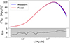 |
Fig. 3. Mean clustering with its standard deviation of the Planck 2018 25 boxes using the median HOD. In red, ξ0 is computed using Eq. (8) with a fixed LoS, and in blue using Eq. (3) with a varying midpoint LoS. In the latter case, in order to get a realistic clustering, we place the observer at the centre of the boxes, and cut a spherical full-sky footprint from z = 0.15 to z = 0.25. The bottom panel shows the residual using the cosmic variance of the (realistic) varying LoS. |
Figure 4 shows the clustering measured for every cosmology and HOD using Eq. (8) and applying RSD along a fixed LoS, which we choose to be the z axis of the box. A sample of the training and test sets is shown in blue and orange, respectively. We choose the separation range to be a logarithmic binning going from the resolution of the simulation 0.3 h−1 Mpc to 60 h−1 Mpc where the flat-sky approximation is still holding. Hereafter, we define Xs as the vector containing those separations (used in Sect. 3). To reduce shot noise, we populate five times the halos using the same HOD model, only changing the random seed, and we average their clustering.
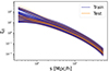 |
Fig. 4. Emulator training and test sets in blue and orange, respectively. The clustering for every cosmology and HOD is measured using Eq. (8) and by applying RSD along a fixed LoS, which we choose to be the z axis of the box. |
Although ABACUSSUMMIT covers a large volume, the training and test cosmology boxes are run with the same initial phase, and the measured clustering is still subject to cosmic variance. To quantify the uncertainties on our measurements, we measure the 2PCF on 1400 of the small Planck 2018 boxes using the median HOD and rescaling the volume, and build the covariance matrix Ccosmic. The corresponding correlation matrix is shown in Fig. 5. We see that, while the scales below a few h−1 Mpc are almost uncorrelated, the large-scale correlations should not be neglected.
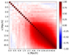 |
Fig. 5. Correlation matrix of the 2PCF monopole computed from 1400 small box realisations of the Planck 2018 cosmology, and using the median HOD. The covariance is rescaled to match the volume of the base boxes. |
3. Multi-scale Gaussian process model
In the following sections, we give a brief description of the GP formalism. We also introduce our new model, which allows every scale to be considered at the same time. For a more complete discussion on the GP, see Reid & White (2011).
3.1. Standard GP regression model
Let  be a training set composed of n pairs of d-dimension input parameter vectors xi and scalar observations yi. Let X be the n × d matrix concatenating every input vector and Y an n column vector. We suppose that the observed values yi are given by
 (9)
(9)
where f is the true underlying mapping function we wish to learn and ϵ is an additive noise following an independent identically distributed Gaussian distribution with mean zero and variance  :
:
 (10)
(10)
where I is the identity matrix. We assume that the mapping function can be described as
 (11)
(11)
where Φ(x) is a set of nf feature functions (e.g. polynomials Φ(x)=(||x||, ||x||2, ||x||3, …, ||x||nf)) mapping the d-dimensional input vector into an nf-dimensional feature space, and w is an nf-dimension vector of unknown weight (and with unknown parameters). This model is a linear function of w for any set of feature functions, and is therefore easier to handle analytically in the training process for instance.
The likelihood of observing Y for a set of input parameters X and weights w can then be written as following a Gaussian distribution:
 (12)
(12)
Choosing a Gaussian prior with zero mean and covariance Σ for the weights,
 (13)
(13)
and following Bayes’ theorem, we can write the posterior distribution over the weights as
 (14)
(14)
where p(Y|X) is the evidence or marginal likelihood.
Making n* predictions f* for a new set of input vectors X* (with X* an n* × d matrix) requires that we marginalise over the weight distributions. The evidence is simply a normalisation constant. Using the Gaussian properties of the prior and likelihood, an analytical expression for the posterior distribution of the prediction can be derived. This latter is expressed as:
 (15)
(15)
where
 (16)
(16)
 (17)
(17)
and Φ = Φ(X) and Φ* = Φ(X*). This posterior is a normal probability distribution over a function space. We note that making a prediction at some new location of the input space is equivalent to analytically performing a Bayesian inference. Thanks to the linearity of the model and the Gaussian assumptions, the posterior probability can be analytically computed.
Let us now define the kernel k(x, x′) = Φ(x)⊤ΣΦ(x′) (we note that k(x, x′) returns a scalar). Doing so allows us to switch from the weight-space view to the so-called function-space view. The expressions for the mean and covariance of the model posterior become:
 (18)
(18)
where K(X, X*) denotes the n × n* covariance matrix built by evaluating the kernel k(x, x*) for the different values of x and x′ (i.e. Kij = k(xi, x*j)).
Specifying a family of feature functions, and letting their number nf go to infinity leads to a compact form of kernel. The most popular in the literature (obtained using Gaussian feature functions) is the squared exponential kernel,
 (19)
(19)
or the Matern kernel,
 (20)
(20)
These are stationary kernels; that is, functions of the distance between two points in the input space, commonly defined as r(x, x′) = (x − x′)⊤M(x − x′) with M = l−2I, where l is a d-dimensional vector containing characteristic length-scales across each dimension of the input space. A large value for some component of l (compared to the input space variance) describes a smoothly varying signal in the corresponding dimension, allowing a larger range on interpolation. In practice, every kernel is also scaled by an additional hyperparameter σ2 to account for the signal amplitude in the output space. We note that the sum or product of different kernels also gives a valid kernel. The training of the GP consists in choosing one or more kernels and inferring the hyperparameters θ = {l, σ} from the input parameter matrix X and their corresponding output observations Y. This is equivalent to a two-level hierarchical Bayesian inference, where Eq. (14) is rewritten as
 (21)
(21)
Now, maximising the posterior probability for new predictions requires that we maximise the evidence p(Y|X,θ). This term now acts as a likelihood in the second level of the hierarchical Bayesian inference. The posterior over the hyperparameters can then be expressed as
 (22)
(22)
where p(θ) is the hyper-prior and p(Y|X) is the hyper-evidence. This second level inference is usually not analytically tractable and requires algorithmic maximisation of the log-likelihood:
![Mathematical equation: $$ \begin{aligned} \log \left[ p ( Y|X, \boldsymbol{\theta } ) \right]&= -\frac{1}{2} Y^\top \left( K(\boldsymbol{x},\boldsymbol{x}) + \sigma _n^2 I\right)^{-1}Y \nonumber \\&\quad - \frac{1}{2} \log \left|K(\boldsymbol{x},\boldsymbol{x}) + \sigma _n^2 I \right| - \frac{n \log (2\pi )}{2}. \end{aligned} $$](/articles/aa/full_html/2024/04/aa48640-23/aa48640-23-eq25.gif) (23)
(23)
The first term on the right-hand side of Eq. (23) describes the goodness of the fit, while the second term is the complexity penalty, which is independent of the observables Y, and allows GP models to (partially) avoid overfitting. We recall the standard result for the gradient of the log-likelihood with respect to a given hyperparameter θi:
 (24)
(24)
with  and
and  .
.
Training a GP (learning the hyperparameters) requires that we compute this likelihood and its gradient several times, which involves obtaining the inverse and the determinant of the n × n matrix Ky. For a training set larger than a few thousand samples, these operations can become computationally prohibitive. For example, considering our case described in Sect. 2, this matrix would have n = nΩ × nHOD × ns = 88 × 600 × 30 ∼ 106, where nΩ, nHOD, and ns are the number of sampled cosmologies, HODs, and separations, respectively.
3.2. Multi-scale GP model
To overcome the issue of large matrix inversions for the standard GP, we can use a particular way of sampling the training data input parameters. This is a process known as Kronecker GP modelling, as is described below.
Let the input parameter matrix of the training set X be composed of n samples of d dimensions. If this matrix can be decomposed as a Kronecker product, X = X1 ⊗ X2, where X1 and X2 have smaller dimensions (n1 × d1 and n2 × d2 respectively) with n = n1 × n2 and d = d1 + d2. This decomposition is only possible if the training set is grid-sampled (e.g. the same HOD parameters are repeated for each set of cosmological parameters), which is suboptimal, but as a result the covariance kernel can be computed as a Kronecker product of two lower-dimension matrices K = K1 ⊗ K2.
This structure allows us to make use of the algebraic properties of Kronecker products. If K is positive definite, it can be written as a principal component decomposition K = QΛQ⊤, where Q = Q1 ⊗ Q2 and Λ = Λ1 ⊗ Λ2, with  , with every Λ matrix diagonal. Thus, every calculation can be performed in subdimensional space. Such a model was implemented in the Python library GPY
3 but only for Kronecker decompositions into two subspaces. Tamone et al. (2020) gives a generalisation of this framework to k decompositions
, with every Λ matrix diagonal. Thus, every calculation can be performed in subdimensional space. Such a model was implemented in the Python library GPY
3 but only for Kronecker decompositions into two subspaces. Tamone et al. (2020) gives a generalisation of this framework to k decompositions  , but this latter is only valid for a diagonal uncorrelated noise matrix N = σ2I.
In this work, we extended this framework to general correlated noise covariance matrices of the form  . This is important in cluster modelling because the noise covariance matrices are generally far from being diagonal, as seen in Fig. 5. The essential step is now to compute the inverse and the determinant of (K+N) in Eq. (23). Assuming a Kronecker-structured training set and performing the decompositions
  , we can derive
 (25)
(25)
where we use different properties of the Kronecker product, and define the projected matrices  , which once built can be decomposed as
  .
.
Now, building  is trivial as Λi are all diagonal matrices. Moreover,
  , and therefore the n × n diagonal matrix (Λ+I) is easily built and inverted. Additionally,
  and
and  , and so the determinant from Eq. (23) is simply the product of the eigenvalue products |S−1/2||Λ+I||S−1/2|. The goodness-of-fit term is computed by iteratively using the KRONMVPROD algorithm (described in Tamone et al. 2020), which evaluates operations of the form
  where b is a column vector.
We also require the evaluation of log-likelihood gradients. The first term of Eq. (24) can be easily computed as the hyperparameters are specific to a particular subdimension d, and therefore to a kernel Kd; that is,
 (26)
(26)
while the second term of Eq. (24) can be computed using the cyclic properties of the trace operator:
 (27)
(27)
with  . The last terms in the above equations are given by
 (28)
(28)
We provide an implementation of this model using the GPY framework and based on JAX GPU parallelisation for algebra operations, which is publicly available as the MKGPY 4 package.
3.3. Application to galaxy clustering
To apply this model to our observable, we decompose the parameter space as a gridded structure X = XΩ ⊗ XHOD ⊗ Xs. Specifically, as mentioned in Sect. 2.2, we measure the correlation function on the same scales using the same HOD sampling for every cosmology, allowing us to decompose the signal and noise covariances as
 (29)
(29)
We find that the optimal signal kernels (maximising the log-likelihood) are simply two Matern3/2 kernels for cosmological and HOD spaces and a squared exponential kernel for the scale space. This choice of modelling leads to 16 signal hyperparameters θ = {lΩ,lHOD,ls,σ}, which include 9 lengthscales for the cosmological parameters lΩ, 5 for the HOD parameters lHOD, one for the separations ls, and one overall variance of the signal σ. For the noise kernels, we chose Ns to be the fixed covariance matrix of the 2PCF monopole computed from the 1400 small boxes (Fig. 5). For the cosmological and HOD noise kernels, we chose diagonal heteroscedastic kernels of the form N(x, x′) = σn(x)2δD(x − x′)I, allowing a different variance for every HOD and cosmological configuration. We allow σn to be fully parameterised vectors, leading to 88 noise hyperparameters for each cosmology and 600 for each HOD. Those noise hyperparameters (σnΩ,σnHOD) are fitted along with the signal hyperparameters θ.
To avoid mathematical overflow and to simplify the hyperparameter learning, we normalise each dimension i of the input and output training sets as follows:
 (30)
(30)
where XΩ and XHOD are normalised to be distributed in the range [0,1]. Because we use stationary kernels k(x, x′) = k(|x − x′|), we need to make sure that the variance of the signal is roughly constant as a function of the input x, which is not the case along the subspace Xs. For this input dimension, we use a logarithmic transformation to flatten the signal before applying the normalisation. We also normalise the output training set Y to be normally distributed around zero with a variance of one; because the 2PCF spans a large range of magnitudes, we also apply a logarithmic transformation before doing so:
 (31)
(31)
The covariance matrix used as Ns must also be projected in the normalised space. To do so, we use the error propagation,
 (32)
(32)
with J the mapping Jacobi matrix  computed for the mean of the 1400 small boxes. Once the emulator is trained, every new input configuration Xtest should be normalised using Eq. (30), and every model prediction μf and its covariance Σf (Eq. (18)) should be transformed back into the real space using Eqs. (31) and (32).
The hyperparameters are optimised using the SCIPY gradient-based algorithm LBFGS with ten random initialisations and selecting the best-fit hyperparameters yielding the highest likelihood. To compare performances, we train both the standard GP, where each separation is treated independently (as separate emulators), and our new multi-scale GP. We employ the same kernels, normalisation, and optimisation method.
4. Emulator performance
In this section, we compare the performances of two emulators: first, the independent Gaussian process model (IGP), where each scale s of the correlation function ξ(s) has its own independent GP depending on cosmological and HOD parameters; and second, our multi-scale Gaussian process model (MGP), which is able to predict the full model for ξ(s) as well as an associated non-diagonal model covariance.
4.1. Prediction accuracy
We computed predictions for the test set composed of 20 HOD × 6 cosmologies (see Sect. 2 for details) using both IGP and MGP models, and compared with their observed correlation function monopoles. Figure 6 describes the IGP and MGP performances using the full test set. The grey lines show the relative difference between the MGP emulator prediction and the expected values from the test set as a percentage. The black dotted line corresponds to a 1% deviation. The blue and green lines are the median of those deviations for the MGP and IGP models, respectively, reaching a subpercent precision for both models on most of the scales. However, the correlation functions of our test set are noisy, which is due to cosmic variance and shot noise, and so we do not expect the difference Δ ≡ ξemu − ξtrue to be smaller than the estimated uncertainty of ξtrue . The red dashed line shows the median of  as a percentage, with σ being the diagonal of Ccosmic . A difference smaller than this reference would indicate overfitting of the particular initial phase of the simulations, while larger differences would show that the prediction performance is poor. Both MGP and IGP models seem to be slightly overfitting the initial phase for the large scales, but follow the expected accuracy on small scales. We note that for the very small scales, the MGP is overfitting the test set to a lesser extent than the IGP. We see that the relative error of the full sample in grey varies around the cosmic variance expectation. We note that the dotted red line corresponds to the cosmic variance of the central cosmology and HOD. The wide HOD scatter causes large variations in the clustering amplitude and therefore in the cosmic variance.
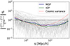 |
Fig. 6. Grey lines show the relative difference between the MGP emulator prediction and the expected values for the full test set, as a percentage difference. The blue and green lines are the median of those deviations for the MGP and IGP models, respectively. The black dotted line corresponds to a 1% deviation. The red dotted line shows the median of |σ/ξtrue| as a percentage. Here, σ2 is the cosmic variance computed for the Planck 2018 cosmology and median HOD. |
4.2. Robustness to cosmic variance
Our models were trained on correlation functions from simulations run with different cosmologies and HOD parameters, but all starting from the same initial phase. Overfitting this particular phase could potentially bias our clustering predictions on simulations with different initial phases. We tested this issue with 25 phase realisations of AbacusSummit run with the same Planck 2018 cosmology and the same set of HOD parameters.
Gaussian processes provide not only a prediction for a model, but also an estimate of the model uncertainty, which depends on the input parameters θ. This uncertainty is expressed as a covariance matrix, denoted Cemu(θ). When performing inferences on real data, this model covariance has to be added to the measurement uncertainty for the considered scales Ccosmic as:
 (33)
(33)
We deliberately dropped the dependency of Ccosmic on θ as it is often considered fixed during inferences. Figure 7 shows the difference Δ between the 25 measurements and predictions from both the MGP (blue) and the IGP (green) emulators. The red dashed line displays the cosmic variance level while blue and green lines show the total variance (model + cosmic) according to Eq. (33). We see that for intermediate scales, Δ is larger than the cosmic variance level, while using Ctot lowers the deviation to less than 1σ. We also note that for this example the variance of the MGP is larger than that of the IGP; however, Fig. 7 only presents the diagonal elements of the covariance matrices.
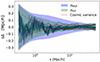 |
Fig. 7. Difference between the emulators prediction and the 25 realisations of Planck 2018 cosmology with the median HOD in blue and green lines for the MGP and IGP, respectively. The red dashed line describes the cosmic variance level. The total variances, including the emulator variance predictions, are shown with the blue and green shaded area. |
Figure 8 shows the total (model + cosmic) correlation matrix of the MGP. We note that compared to Ccosmic alone (Fig. 5), the small scales are now significantly correlated. The predicted covariance matrix of the IGP is diagonal by construction, and so cannot account for such correlations, potentially affecting cosmological constraints. We investigate this issue in Sect. 5.
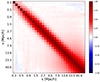 |
Fig. 8. Total correlation matrix of the MGP, including the model uncertainty prediction Ctot = Ccosmic + Cemu(θΩ, θhod). The measurement uncertainty Ccosmic was evaluated for the Planck 2018 cosmology with the median HOD using the 1400 small boxes. |
The clustering measurements for the 25 mocks are shown in the top panel of Fig. 9 with the average shown with a red dotted line. The bottom panel describes the 25 residuals for both IGP (green) and MGP (blue) predictions, with Δ = ξemu − ξtrue, and L−1 being the Cholesky decomposition of the inverse of the total covariance Ctot. This residual metric is useful as it takes into account the correlations between scales. The shaded areas correspond to 1σ and 2σ deviations. For most of the scales, both MGP and IGP models are able to reproduce the clustering for the different realisations within a 1σ deviation. For every scale, the residuals are within a 2σ deviation. It seems that for both models the predicted uncertainty Cemu solves the initial condition phase problem. In the following section, we study the recovering of the cosmological and HOD parameters.
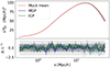 |
Fig. 9. Emulator performance on mocks with different phase. In the upper panel the 25 realisations of Planck 2018 cosmology using the median HOD are shown in grey. The average is shown in red dotted line. The 25 residuals for both IGP (green) and MGP (blue) predictions are shown in the bottom panel. L−1 is the Cholesky decomposition of the inverse of Ctot. The grey shaded areas correspond to 1σ and 2σ deviations. |
5. Cosmology recovery and constraints
In this section, we describe the performances of our models in recovering unbiased cosmological and HOD parameters. We used the clustering measured on 25 realisations of the Planck 2018 cosmology using the same median HOD parameters.
5.1. Parameter inference using the emulator model
The parameter inferences are performed by running MCMC chains with the library EMCEE, using a flat prior corresponding to Table 1 and a standard Gaussian log-likelihood defined as
 (34)
(34)
where μ is the data vector, m(θ) is the model prediction for a given set of parameters θ = (θΩ,θhod), and Ctot(θ) is the total (model + cosmic ) covariance defined in Eq. (33). Compared to a ‘normal’ cosmological inference, the terms  and log|Ctot(θ)| must be computed for every iteration because of the emulator covariance dependence on the parameters. To do so efficiently, we make use of the fast and stable Cholesky decomposition.
For a given set of cosmological parameters, we can infer the corresponding growth rate f. The uncertainty on the measured growth rate is simply propagated as  , where CΩij is the covariance of the inferred cosmological parameters. We use the JACOBI
5 Python library to compute the gradient of our model.
, where CΩij is the covariance of the inferred cosmological parameters. We use the JACOBI
5 Python library to compute the gradient of our model.
5.2. Cubic boxes: Average fit
We first tested the performance of both IGP and MGP models in recovering the parameters of interest when fitting a high-precision measurement; that is, with an average stack of the 25 correlation function monopoles, corresponding to a volume of 200 (h−1 Gpc)3. We used the likelihood defined in Eq. (34), divided the sample covariance Ccosmic by 25, and ran two inferences with and without using the emulator-predicted covariance Cemu for each model.
Figure 10 shows the 68% and 95% confidence regions obtained for the cosmological and HOD parameters. The true values are shown by the dotted lines. We observe several interesting features. First, neglecting the model covariance leads to strongly biased results for the IGP with very sharp posterior distributions, while the MGP performs significantly better though yielding multimodal posteriors. Second, using the model covariance allows us to recover unbiased results for all cosmological parameters within one sigma for both models. Third, while MGP and IGP contours are consistent, the MGP model gives tighter constraints on cosmological parameters, and the IGP model gives tighter constraints on the HOD parameters. We also see several local maxima in the posterior distributions, especially in the green IGP contours. When sampling cosmological parameters far from those used in the training process of the GPs, we see larger model covariances while fitting the data points. This can also be seen as the goodness-of-fit term being counterbalanced by the determinant in the likelihood. Ignoring the model covariance can cause the fitter to converge towards a point that – when considering the total covariance – is found to be only a local maxima in the log likelihood.
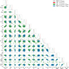 |
Fig. 10. Posterior distribution of the cosmological and HOD parameters obtained after running MCMC inference on the average stack of the 25 correlation functions with Planck 2018 cosmology and the median HOD. The results obtained using the IGP model with and without the model covariance prediction are shown in green and red, respectively, and those obtained using the MGP model with and without the model covariance prediction are shown in blue and black, respectively. The true parameters are shown by the black dotted lines. |
Figure 11 compares the best fits of the MGP and IGP models in blue and green, respectively. The bottom panel displays the residuals, using the Cholesky decomposition matrix to account for correlations between scales. The 1σ deviation limit is set by the grey shaded area. For the MGP model, we get a reduced chi squared of  and for the IGP we obtain
  . These large
  values are due to the large volume probed by the average of 25 simulations. These
  values and the bottom panel of Fig. 11 show that the data are much better adjusted by the MGP model over all scales.
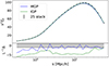 |
Fig. 11. The 25 realisations of Planck 2018 cosmology with the median HOD in grey. The average is shown with a red dotted line and the MGP prediction is shown in blue. The 25 residuals for both IGP (green) and MGP (blue) predictions are shown in the bottom panel. L−1 is the Cholesky decomposition of the inverse of Ctot. |
5.3. Cubic boxes: 25 individual fits
In order to obtain a statistically significant measurement of the accuracy and potential biases of our models, we fit each of the 25 boxes separately, corresponding to a probed volume comparable to current surveys. The cosmic covariance matrices were normalised to account for this change in volume. Figure 12 shows the reduced chi-squared  , the best-fit growth rate parameter f, and their estimated uncertainties σf. The derived cosmological parameters along with their inferred uncertainties are shown in Fig. 13 and the same for the HOD parameters in Fig. 14. Table 2 reports some summary statistics from those results, where ⟨Δp⟩ is the difference between the true and best-fit value for parameter p; ⟨σp⟩ is the average over the 25 realisations of the (symmetrised) 1σ confidence level; and std(p) is the standard deviation of the estimated parameter p over the 25 fits. We note that the bias in the growth-rate measurement is reduced with our MGP model, and that both models give consistent results, recovering the growth rate within 1σ. The reduced chi-squared distributions are similar, but with this sample the IGP model gives a better fit, on average, with
  , while we have
  for MGP for (30 − 14)=16 degrees of freedom. Although it is hard to draw conclusions because of the limited size of the sample, in both cases the mean estimated error ⟨σf⟩ does not exactly match the standard deviation of the best-fit parameters std(p), but is conservatively larger. We also see that our MGP model yields smaller dispersion and results in tighter constraints on f.
Summary statistics for the fits of the 25 cubic mocks with Planck 2018 cosmology and the median HOD.
Figure 13 showcases similar results for the cosmological parameters. Both models are able to retrieve the right parameters within 1σ, but the MGP returns smaller bias, smaller dispersion, and tighter constraints for all parameters except the number of ultrarelativistic species Nur, which is poorly constrained. In particular, the uncertainty on amplitude parameter σ8 is reduced by a factor of greater than 4, while reducing the bias on the best-fit value. For the HOD parameters illustrated in Fig. 14, we also get unbiased measurements. Once again, the bias and the dispersion for the best-fit values are overall reduced with the MGP; however, the IGP gets tighter constraints. It therefore seems that using the correlation between scales helps to constrain the cosmology rather than the HOD parameters as the HOD signal is mainly in the small scales where the cosmic covariance is almost diagonal (see Fig. 5), while all scales are affected by cosmological parameters.
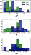 |
Fig. 12. Reduced chi squared, best-fit growth rate, and corresponding uncertainties resulting from the separate fits of the 25 cubic mocks with Planck 2018 cosmology and the median HOD. Results using the MGP and IGP models are shown in blue and green, respectively. The true parameter values are shown with a red dotted line. |
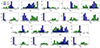 |
Fig. 13. Best-fit cosmological parameters along with the corresponding uncertainties on the 25 cubic mocks with Planck 2018 cosmology and the median HOD. Results using the MGP and IGP models are shown in blue and green, respectively. The true parameters values are shown by a red dotted line. |
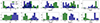 |
Fig. 14. Best-fit HOD parameters along with the corresponding uncertainties on the 25 cubic mocks with Planck 2018 cosmology and the median HOD. Results using the MGP and IGP models are shown in blue and green, respectively. The true parameters values are shown by a red dotted line. |
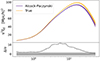 |
Fig. 15. AP effect on the observable. Top panel: mean clustering with its standard deviation of the 25 mocks with Planck 2018 cosmology, the median HOD, and a spherical full-sky footprint from z = 0.15 to z = 0.25. The true and AP-distorted clustering are shown in orange and indigo, respectively. The bottom panel shows the residual using the cosmic variance of the varying LoS clustering. |
5.4. Observational effects: Wide angle and AP
We validated the MGP model on cubic mocks similar to the simulations used to train the emulators and show that it performs significantly better than the standard IGP. Now we wish to test the constraining power and accuracy of the MGP model on more realistic measurements.
For each of the 25 realisations, we placed the observer at the centre of the box. As the snapshot describes the clustering at redshift z = 0.2, we select galaxies at redshifts 0.15 < z < 0.25 from the observer, in order to avoid making large changes to the observed clustering. We consider each survey to cover the full sky. We used the Landy-Szalay estimator of Eq. (3) to compute correlation functions. The measurement of the 2PCF requires the choice of a specific fiducial cosmology to convert redshifts into comoving distances. Differences between the fiducial and the true cosmology lead to distortions in the measured clustering, which is known as the Alcock-Paczynski (AP) effect (Alcock & Paczynski 1979). This effect is often neglected when building an emulator (Yuan et al. 2022b; Planck Collaboration VI 2020) as it is small on very small scales. Moreover, modelling the AP distortion requires either one extra parameter in the training input space or a continuous model over different scales for interpolation. By construction, our MGP model is more adapted to building a continuous model than the IGP, and such a model can be evaluated at any scale within the training range.
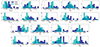 |
Fig. 17. Best-fit cosmological parameters along with the corresponding uncertainties on the 25 mocks with spherical full sky footprint from z = 0.15 to z = 0.25, AP distortion, Planck 2018 cosmology, and the median HOD. Results using the MGP with and without modelling AP distortions are shown in cyan and blue, respectively. The true parameter values are pointed by a red dotted line. |
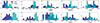 |
Fig. 18. Best-fit HOD parameters along with the corresponding uncertainties on the 25 mocks with spherical full-sky footprint from z = 0.15 to z = 0.25, AP distortion, Planck 2018 cosmology, and the median HOD. Results using the MGP with and without modelling AP distortions are shown in cyan and blue, respectively. The true parameter values are shown by a red dotted line. |
If the choice of fiducial cosmology is not far from the true cosmology, the AP effect can be modelled with two parameters, which scale the radial and angular separations. However, as we are only using the monopole of the 2PCF, we only have access to isotropic information. We use the isotropic dilatation parameter αV described by Navarro et al. (1997) to scale separations as
 (35)
(35)
where
 (36)
(36)
with the isotropic distance defined as a combination of the Hubble distance (radial) DH(z)=c/H(z) and the comoving angular distance DM(z)=(1 + z)DA(z):
![Mathematical equation: $$ \begin{aligned} D_V(z) = \left[ z D_H(z)D_M^2(z) \right]^{1/3}. \end{aligned} $$](/articles/aa/full_html/2024/04/aa48640-23/aa48640-23-eq64.gif) (37)
(37)
We picked cosmology c177 of the ABACUSSUMMIT suite as a fiducial cosmology; it is different from the true one (Planck 2018), resulting in a 2% variation in the isotropic dilatation parameter αv ≈ 1.02. We measure the clustering of the 25 realisations of our survey-like mocks using both the true and c177 fiducial cosmologies. The average monopoles along with the residual (using the cosmic variance of the survey-like mocks) are shown in Fig. 15. Although the cosmic variance is larger for the survey-like mocks compared to the cubic box measurements – which is due to the reduced volume –, the AP distortions lead to significant deviations for every scale, up to 10σ for scales of a few h−1 Mpc.
To assess whether or not ignoring the AP distortions can lead to biased cosmological constraints, we fit the 25 realisations of the AP distorted clustering separately using the MGP model with and without (setting αV = 1) accounting for the AP distortions. We refer to the former as MGPαV. In both cases, we rescale the sample covariance matrix with the corresponding spherical volume. We also compare the impact of ignoring the AP effect using MGP and IGP in Appendix A.
Figure 16 displays the distribution of reduced chi-squared, best-fit growth rate f, and their estimated uncertainties σf. The best-fit cosmological and HOD parameters with their uncertainties are shown in Figs. 17 and 18, respectively. Table 3 shows summary statistics as in Table 2, but now for the survey-like mocks. With a significantly larger cosmic variance, the models better fit the data, and therefore the reduced chi-squared distributions are less spread and more centred on one compared to the cubic box fits. The data points are also better described when accounting for AP distortions; the mean of the distribution is ⟨ for MGPαV and
  for MGP for (30 − 14)=16 degrees of freedom. In both cases, we recover the expected growth rate within 1σ, though ignoring the AP effect increases the bias by a factor of ten and leads to larger error bars, and also with best-fit values for f that are more scattered. We also note that compared to the previous cubic box fits, although the cosmic variance of the survey-like mocks is larger, the growth rate is more constrained in both cases. We see similar results in Fig. 17 for the cosmological parameters: when considering AP distortion in the modelling, we reduce the bias and obtain tighter constraints. However, the dark energy parameters w0 and wa appear as an exception, where although MGPαV gives tighter constraints, the bias is larger than when using MGP. However, as those parameters are weakly constrained, the difference in the growth-rate measurement accuracy between the two models mainly comes from the ωm and h parameters. For the HOD parameters showcased in Fig. 18, in both cases we have unbiased results for every parameter. However, as HOD parameters are mostly constrained at small scales, where the AP effect is less important, the MGPαV model does not bring any substantial improvement, and even gives looser constraints than the MGP without AP modelling on average.
Summary statistics for the fits of the 25 mocks with spherical full-sky footprint from z = 0.15 to z = 0.25, Planck 2018 cosmology, and the median HOD, where the clustering was measured using cosmology C177 of the ABACUSSUMMIT suite as fiducial cosmology resulting in an isotropic dilatation parameter αv ≈ 1.02.
6. Conclusions
In this work, we review the standard methodology for training an emulator model for galaxy clustering at non-linear scales from a suite of dark matter simulations. We introduce a new Gaussian process model that allows efficient extension of the input parameter space dimension and accounts for correlated noise.
As a proof of concept for our model, we emulated the redshift space 2PCF of galaxies over the input space X = XΩ ⊗ XHOD ⊗ Xs, allowing an additional interpolation over a continuous range of scales, and making use of the well-known correlations between them, both in the signal and the noise. We implemented our multi-scale Gaussian process model (MGP) as well as the standard approach, which consists in constructing independent Gaussian processes (IGPs) for each separation. We used 88 cosmologies, 600 HODs, and 30 separation scales as a training set, all measured in the ABACUSSUMMIT suite of n-body simulations. The input parameter space of the resulting models is composed of nine cosmological parameters, five HOD parameters, and the set of separations of the 2PCF.
After validating the predictive accuracy of our trained model on a test set with six cosmologies and 20 HODs, we ran inferences using MCMC to check the robustness and constraining power of our models. In a high-precision setting, where we used the average 2PCF of 25 realisations, ignoring the predicted uncertainties of our GP models can lead to biased results, especially with the IGP model. We also demonstrate that both models are able to recover the expected HOD parameters. Marginalising over such parameters, we are able to obtain unbiased cosmological constraints. Our MGP model returns more accurate and precise constraints on the cosmological parameters than the IGP.
Moreover, we show that Alcock-Paczynski distortions can become important compared to the cosmic variance at intermediate scales for the redshifts we are testing. Neglecting this effect in an emulator model, as has been done in previous works, contributes to loosening the constraints and increasing the bias on the growth-rate measurement.
The parameter space of such emulator models could also be extended to higher dimensions to be able to interpolate and marginalise over systematic quantities, extended HOD models, selection effects, different redshift bins, and more. There remain some drawbacks to using a training set with a large number of dimensions. First, building the training set is expensive. Second, although a Kronecker GP model with a very large number of training points can be trained relatively quickly, the predictions of the model covariance can be slow. It is also important to reiterated that for galaxies at lower redshift, building a model requires more realistic simulations that reproduce redshift evolution (light cone) to account for wild angle effects. Such a model would also need to be validated on realistic mocks using different galaxy–halo connections before application to real measurements.
Our MGP model could be used in future works to emulate a larger set of galaxy clustering observables and their cross correlations, such as: galaxy and peculiar velocity auto- and cross-correlations, galaxy clustering, weak lensing, and so on. Accurate models of these correlations are essential in the era of high-precision measurements from surveys such as DESI or Euclid.
While a z = 0.1 snapshot exists for ABACUSSUMMIT, the smaller boxes for covariance matrix estimations were not available.
Acknowledgments
We would like to thank Zhongxu Zhai, Will Percival, Corentin Ravoux for useful discussions. The project leading to this publication has received funding from Excellence Initiative of Aix-Marseille University – A*MIDEX, a French “Investissements d’Avenir” program (AMX-20-CE-02 – DARKUNI).
References
- Alam, S., Ata, M., Bailey, S., et al. 2017, MNRAS, 470, 2617 [Google Scholar]
- Alam, S., Aubert, M., Avila, S., et al. 2021, Phys. Rev. D, 103, 083533 [NASA ADS] [CrossRef] [Google Scholar]
- Alcock, C., & Paczynski, B. 1979, Nature, 281, 358 [NASA ADS] [CrossRef] [Google Scholar]
- Bautista, J. E., Paviot, R., Vargas Magaña, M., et al. 2021, MNRAS, 500, 736 [Google Scholar]
- Blanton, M. R., Bershady, M. A., Abolfathi, B., et al. 2017, AJ, 154, 28 [Google Scholar]
- Carlson, J., Reid, B., & White, M. 2013, MNRAS, 429, 1674 [NASA ADS] [CrossRef] [Google Scholar]
- Carrasco, J. J. M., Foreman, S., Green, D., & Senatore, L. 2014, JCAP, 2014, 057 [CrossRef] [Google Scholar]
- Chapman, M. J., Mohammad, F. G., Zhai, Z., et al. 2022, MNRAS, 516, 617 [NASA ADS] [CrossRef] [Google Scholar]
- Colless, M., Peterson, B. A., Jackson, C., et al. 2003, arXiv e-prints [arXiv:astro-ph/0306581] [Google Scholar]
- Dawson, K. S., Schlegel, D. J., Ahn, C. P., et al. 2013, AJ, 145, 10 [Google Scholar]
- Dawson, K. S., Kneib, J.-P., Percival, W. J., et al. 2016, AJ, 151, 44 [Google Scholar]
- de Mattia, A., Ruhlmann-Kleider, V., Raichoor, A., et al. 2021, MNRAS, 501, 5616 [NASA ADS] [Google Scholar]
- DeRose, J., Wechsler, R. H., Tinker, J. L., et al. 2019, ApJ, 875, 69 [NASA ADS] [CrossRef] [Google Scholar]
- DESI Collaboration (Aghamousa, A., et al.) 2016, arXiv e-prints [arXiv:1611.00036] [Google Scholar]
- DESI Collaboration (Aghamousa, A., et al.) 2022, AJ, 164, 207 [NASA ADS] [CrossRef] [Google Scholar]
- Drinkwater, M. J., Jurek, R. J., Blake, C., et al. 2010, MNRAS, 401, 1429 [CrossRef] [Google Scholar]
- du Mas des Bourboux, H., Rich, J., & Rich, A. 2020, ApJ, 901, 153 [CrossRef] [Google Scholar]
- Eisenstein, D. J., Weinberg, D. H., Agol, E., et al. 2011, AJ, 142, 72 [Google Scholar]
- Euclid Collaboration (Scaramella, R., et al.) 2022, A&A, 662, A112 [NASA ADS] [CrossRef] [EDP Sciences] [Google Scholar]
- Garrison, L. H., Eisenstein, D. J., Ferrer, D., Maksimova, N. A., & Pinto, P. A. 2021, MNRAS, 508, 575 [NASA ADS] [CrossRef] [Google Scholar]
- Gil-Marín, H., Bautista, J. E., Paviot, R., et al. 2020, MNRAS, 498, 2492 [Google Scholar]
- Guzzo, L., Scodeggio, M., Garilli, B., et al. 2014, A&A, 566, A108 [NASA ADS] [CrossRef] [EDP Sciences] [Google Scholar]
- Hadzhiyska, B., Eisenstein, D., Bose, S., Garrison, L. H., & Maksimova, N. 2021, MNRAS, 509, 501 [NASA ADS] [CrossRef] [Google Scholar]
- Hou, J., Sánchez, A. G., Ross, A. J., et al. 2021, MNRAS, 500, 1201 [Google Scholar]
- Hou, J., Bautista, J., Berti, M., et al. 2023, Universe, 9, 302 [NASA ADS] [CrossRef] [Google Scholar]
- Howlett, C., Ross, A. J., Samushia, L., Percival, W. J., & Manera, M. 2015, MNRAS, 449, 848 [NASA ADS] [CrossRef] [Google Scholar]
- Huterer, D. 2023, A&ARv, 31, 2 [NASA ADS] [CrossRef] [Google Scholar]
- Jones, D. H., Saunders, W., Colless, M., et al. 2004, MNRAS, 355, 747 [NASA ADS] [CrossRef] [Google Scholar]
- Kobayashi, Y., Nishimichi, T., Takada, M., Takahashi, R., & Osato, K. 2020, Phys. Rev. D, 102, 063504 [NASA ADS] [CrossRef] [Google Scholar]
- Kobayashi, Y., Nishimichi, T., Takada, M., & Miyatake, H. 2022, Phys. Rev. D, 105, 083517 [CrossRef] [Google Scholar]
- Kwan, J., Saito, S., Leauthaud, A., et al. 2023, ApJ, 952, 80 [NASA ADS] [CrossRef] [Google Scholar]
- Landy, S. D., & Szalay, A. S. 1993, ApJ, 412, 64 [Google Scholar]
- Laureijs, R., Amiaux, J., Arduini, S., et al. 2011, arXiv e-prints [arXiv:1110.3193] [Google Scholar]
- Maksimova, N. A., Garrison, L. H., Eisenstein, D. J., et al. 2021, MNRAS, 508, 4017 [NASA ADS] [CrossRef] [Google Scholar]
- Moon, J., Valcin, D., Rashkovetskyi, M., et al. 2023, MNRAS, 525, 5406 [NASA ADS] [CrossRef] [Google Scholar]
- Navarro, J. F., Frenk, C. S., & White, S. D. M. 1997, ApJ, 490, 493 [Google Scholar]
- Neveux, R., Burtin, E., de Mattia, A., et al. 2020, MNRAS, 499, 210 [NASA ADS] [CrossRef] [Google Scholar]
- Pajer, E., & Zaldarriaga, M. 2013, JCAP, 2013, 037 [CrossRef] [Google Scholar]
- Peebles, P. J. E., & Hauser, M. G. 1974, ApJS, 28, 19 [NASA ADS] [CrossRef] [Google Scholar]
- Planck Collaboration VI. 2020, A&A, 641, A6 [NASA ADS] [CrossRef] [EDP Sciences] [Google Scholar]
- Prada, F., Ereza, J., Smith, A., et al. 2023, arXiv e-prints [arXiv:2306.06315] [Google Scholar]
- Rasmussen, C. E., & Williams, C. K. I. 2006, Gaussian Processes for Machine Learning, Adaptive Computation and Machine Learning (Cambridge, Mass: MIT Press) [Google Scholar]
- Reid, B. A., & White, M. 2011, MNRAS, 417, 1913 [NASA ADS] [CrossRef] [Google Scholar]
- Ross, A. J., Samushia, L., Howlett, C., et al. 2015, MNRAS, 449, 835 [NASA ADS] [CrossRef] [Google Scholar]
- Saatci, Y. 2011, PhD Thesis, University of Cambridge, UK [Google Scholar]
- Tamone, A., Raichoor, A., Zhao, C., et al. 2020, MNRAS, 499, 5527 [Google Scholar]
- Taruya, A., Nishimichi, T., & Saito, S. 2010, Phys. Rev. D, 82 [CrossRef] [Google Scholar]
- Villaescusa-Navarro, F., Hahn, C., Massara, E., et al. 2020, ApJS, 250, 2 [CrossRef] [Google Scholar]
- Wang, L., Reid, B., & White, M. 2014, MNRAS, 437, 588 [NASA ADS] [CrossRef] [Google Scholar]
- Weinberg, D. H., Mortonson, M. J., Eisenstein, D. J., et al. 2013, Phys. Rep., 530, 87 [Google Scholar]
- Yoo, J., & Seljak, U. 2015, MNRAS, 447, 1789 [NASA ADS] [CrossRef] [Google Scholar]
- Yuan, S., Garrison, L. H., Eisenstein, D. J., & Wechsler, R. H. 2022a, MNRAS, 515, 871 [NASA ADS] [CrossRef] [Google Scholar]
- Yuan, S., Garrison, L.H., Hadzhiyska, B., Bose, S., & Eisenstein, D. J. 2022b, MNRAS, 510, 3301 [NASA ADS] [CrossRef] [Google Scholar]
- Zhai, Z., Blanton, M., Slosar, A., & Tinker, J. 2017, ApJS, 850, 183 [NASA ADS] [Google Scholar]
- Zhai, Z., Tinker, J. L., Banerjee, A., et al. 2023, ApJ, 948, 99 [NASA ADS] [CrossRef] [Google Scholar]
- Zheng, Z., Coil, A. L., & Zehavi, I. 2007, ApJ, 667, 760 [Google Scholar]
Appendix A: AP effect on IGP fits
We show in section 5.4 that ignoring the AP distortions can lead to a loss of accuracy and precision, especially for the two cosmological parameters of interest, f and σ8. Here, we compare the impact of ignoring the AP distortions using the MGP and IGP models. We note that as the IGP is not able to interpolate over scales, the AP effect is usually ignored in standard analysis (Yuan et al. 2022b; Planck Collaboration VI 2020; Landy & Szalay 1993). While the AP effect could also be modelled using the IGP, this would require that an extra approximated interpolation be performed between the trained scales, both for model and uncertainty estimates. We fit the 25 realisations of the AP distorted clustering separately using both models without modelling the AP distortions. In both cases, we rescale the sample covariance matrix with the corresponding spherical volume. The best-fit values for f and σ8 along with their estimated uncertainties are described in figure 16. The best-fit cosmological and HOD parameters with their uncertainties are shown in figure A.1. Table A.1 shows summary statistics for all cosmological and HOD parameters. We see that when ignoring the AP distortions, although not the case for HOD parameters (the very small scales remain unaffected by the AP effect), the MGP model performs significantly better than the IGP for every cosmological parameter. The IGP model in particular gives constraints on σ8 that are biased by more than 1σ.
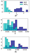 |
Fig. 16. Reduced chi squared, best-fit growth rate, and corresponding uncertainties resulting from the separate fits of the 25 mocks with spherical full-sky footprint from z = 0.15 to z = 0.25, AP distortion, Planck 2018 cosmology, and the median HOD. Results using the MGP with and without modelling AP distortions are shown in cyan and blue, respectively. The true growth-rate value is shown by a red dotted line. |
Summary statistics for the fits of the 25 mocks with a spherical full-sky footprint from z = 0.15 to z = 0.25, Planck2018 cosmology, and the median HOD.
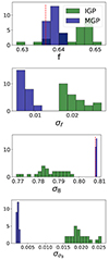 |
Fig. A.1. Best-fit growth rate and corresponding uncertainties resulting from the separate fits of the 25 mocks with spherical full-sky footprint from z = 0.15 to z = 0.25, AP distortion, Planck2018 cosmology, and the median HOD. Results using the MGP and IGP models are shown in blue and green, respectively. The true parameter values are shown by the red dotted line. |
All Tables
Cosmological and HOD parameter names and ranges sampled to build the emulator training and testing sets.
Summary statistics for the fits of the 25 cubic mocks with Planck 2018 cosmology and the median HOD.
Summary statistics for the fits of the 25 mocks with spherical full-sky footprint from z = 0.15 to z = 0.25, Planck 2018 cosmology, and the median HOD, where the clustering was measured using cosmology C177 of the ABACUSSUMMIT suite as fiducial cosmology resulting in an isotropic dilatation parameter αv ≈ 1.02.
Summary statistics for the fits of the 25 mocks with a spherical full-sky footprint from z = 0.15 to z = 0.25, Planck2018 cosmology, and the median HOD.
All Figures
|
Fig. 1. Sampling over the nine-dimensional cosmological space around Planck 2018 ΛCDM. The 88 cosmologies used to train the emulator are shown in blue, while the 6 cosmologies used as a test set are shown in orange. The dark matter density is denoted ωcdm, the baryon density ωb, the clustering amplitude σ8, the dark energy equation of state w(a)=w0 + wa(1 − a), the Hubble constant h, the spectral tilt ns, the density of massless relics Nur, and the running of the spectral tilt αs (Moon et al. 2023). |
| In the text | |
|
Fig. 2. Different forms that take the total occupation of the galaxy for the 600 HOD parametrisation used. The black lines show the mean HOD configuration for ⟨Ncen(M)⟩, ⟨Nsat(M)⟩, and ⟨Ntot(M)⟩. |
| In the text | |
|
Fig. 3. Mean clustering with its standard deviation of the Planck 2018 25 boxes using the median HOD. In red, ξ0 is computed using Eq. (8) with a fixed LoS, and in blue using Eq. (3) with a varying midpoint LoS. In the latter case, in order to get a realistic clustering, we place the observer at the centre of the boxes, and cut a spherical full-sky footprint from z = 0.15 to z = 0.25. The bottom panel shows the residual using the cosmic variance of the (realistic) varying LoS. |
| In the text | |
|
Fig. 4. Emulator training and test sets in blue and orange, respectively. The clustering for every cosmology and HOD is measured using Eq. (8) and by applying RSD along a fixed LoS, which we choose to be the z axis of the box. |
| In the text | |
|
Fig. 5. Correlation matrix of the 2PCF monopole computed from 1400 small box realisations of the Planck 2018 cosmology, and using the median HOD. The covariance is rescaled to match the volume of the base boxes. |
| In the text | |
|
Fig. 6. Grey lines show the relative difference between the MGP emulator prediction and the expected values for the full test set, as a percentage difference. The blue and green lines are the median of those deviations for the MGP and IGP models, respectively. The black dotted line corresponds to a 1% deviation. The red dotted line shows the median of |σ/ξtrue| as a percentage. Here, σ2 is the cosmic variance computed for the Planck 2018 cosmology and median HOD. |
| In the text | |
|
Fig. 7. Difference between the emulators prediction and the 25 realisations of Planck 2018 cosmology with the median HOD in blue and green lines for the MGP and IGP, respectively. The red dashed line describes the cosmic variance level. The total variances, including the emulator variance predictions, are shown with the blue and green shaded area. |
| In the text | |
|
Fig. 8. Total correlation matrix of the MGP, including the model uncertainty prediction Ctot = Ccosmic + Cemu(θΩ, θhod). The measurement uncertainty Ccosmic was evaluated for the Planck 2018 cosmology with the median HOD using the 1400 small boxes. |
| In the text | |
|
Fig. 9. Emulator performance on mocks with different phase. In the upper panel the 25 realisations of Planck 2018 cosmology using the median HOD are shown in grey. The average is shown in red dotted line. The 25 residuals for both IGP (green) and MGP (blue) predictions are shown in the bottom panel. L−1 is the Cholesky decomposition of the inverse of Ctot. The grey shaded areas correspond to 1σ and 2σ deviations. |
| In the text | |
|
Fig. 10. Posterior distribution of the cosmological and HOD parameters obtained after running MCMC inference on the average stack of the 25 correlation functions with Planck 2018 cosmology and the median HOD. The results obtained using the IGP model with and without the model covariance prediction are shown in green and red, respectively, and those obtained using the MGP model with and without the model covariance prediction are shown in blue and black, respectively. The true parameters are shown by the black dotted lines. |
| In the text | |
|
Fig. 11. The 25 realisations of Planck 2018 cosmology with the median HOD in grey. The average is shown with a red dotted line and the MGP prediction is shown in blue. The 25 residuals for both IGP (green) and MGP (blue) predictions are shown in the bottom panel. L−1 is the Cholesky decomposition of the inverse of Ctot. |
| In the text | |
|
Fig. 12. Reduced chi squared, best-fit growth rate, and corresponding uncertainties resulting from the separate fits of the 25 cubic mocks with Planck 2018 cosmology and the median HOD. Results using the MGP and IGP models are shown in blue and green, respectively. The true parameter values are shown with a red dotted line. |
| In the text | |
|
Fig. 13. Best-fit cosmological parameters along with the corresponding uncertainties on the 25 cubic mocks with Planck 2018 cosmology and the median HOD. Results using the MGP and IGP models are shown in blue and green, respectively. The true parameters values are shown by a red dotted line. |
| In the text | |
|
Fig. 14. Best-fit HOD parameters along with the corresponding uncertainties on the 25 cubic mocks with Planck 2018 cosmology and the median HOD. Results using the MGP and IGP models are shown in blue and green, respectively. The true parameters values are shown by a red dotted line. |
| In the text | |
|
Fig. 15. AP effect on the observable. Top panel: mean clustering with its standard deviation of the 25 mocks with Planck 2018 cosmology, the median HOD, and a spherical full-sky footprint from z = 0.15 to z = 0.25. The true and AP-distorted clustering are shown in orange and indigo, respectively. The bottom panel shows the residual using the cosmic variance of the varying LoS clustering. |
| In the text | |
|
Fig. 17. Best-fit cosmological parameters along with the corresponding uncertainties on the 25 mocks with spherical full sky footprint from z = 0.15 to z = 0.25, AP distortion, Planck 2018 cosmology, and the median HOD. Results using the MGP with and without modelling AP distortions are shown in cyan and blue, respectively. The true parameter values are pointed by a red dotted line. |
| In the text | |
|
Fig. 18. Best-fit HOD parameters along with the corresponding uncertainties on the 25 mocks with spherical full-sky footprint from z = 0.15 to z = 0.25, AP distortion, Planck 2018 cosmology, and the median HOD. Results using the MGP with and without modelling AP distortions are shown in cyan and blue, respectively. The true parameter values are shown by a red dotted line. |
| In the text | |
|
Fig. 16. Reduced chi squared, best-fit growth rate, and corresponding uncertainties resulting from the separate fits of the 25 mocks with spherical full-sky footprint from z = 0.15 to z = 0.25, AP distortion, Planck 2018 cosmology, and the median HOD. Results using the MGP with and without modelling AP distortions are shown in cyan and blue, respectively. The true growth-rate value is shown by a red dotted line. |
| In the text | |
|
Fig. A.1. Best-fit growth rate and corresponding uncertainties resulting from the separate fits of the 25 mocks with spherical full-sky footprint from z = 0.15 to z = 0.25, AP distortion, Planck2018 cosmology, and the median HOD. Results using the MGP and IGP models are shown in blue and green, respectively. The true parameter values are shown by the red dotted line. |
| In the text | |
Current usage metrics show cumulative count of Article Views (full-text article views including HTML views, PDF and ePub downloads, according to the available data) and Abstracts Views on Vision4Press platform.
Data correspond to usage on the plateform after 2015. The current usage metrics is available 48-96 hours after online publication and is updated daily on week days.
Initial download of the metrics may take a while.