| Issue |
A&A
Volume 683, March 2024
|
|
|---|---|---|
| Article Number | A183 | |
| Number of page(s) | 9 | |
| Section | Numerical methods and codes | |
| DOI | https://doi.org/10.1051/0004-6361/202348247 | |
| Published online | 19 March 2024 | |
TransientX: A high-performance single-pulse search package
Max-Planck-Institut für Radioastronomie,
Auf dem Hügel 69,
53121
Bonn,
Germany
e-mail: This email address is being protected from spambots. You need JavaScript enabled to view it.
Received:
12
October
2023
Accepted:
24
January
2024
Abstract
Context. Radio interferometers composed of a large array of small antennas possess large fields of view, coupled with high sensitivities. For example, the Karoo Array Telescope (MeerKAT) achieves a gain of up to 2.8 KJy−1 across its >1 deg2 field of view. This capability significantly enhances the survey speed for pulsars and fast transients. It also introduces challenges related to the high data rate, which reaches a few Tb s−1 for MeerKAT, and it requires substantial computing power.
Aims. To handle the high data rate of surveys, we have developed a high-performance single-pulse search software called “TransientX”. This software integrates multiple processes into one pipeline, which includes radio-frequency interference mitigation, dedispersion, matched filtering, clustering, and candidate plotting.
Methods. In TRANSIENTX, we developed an efficient CPU-based dedispersion implementation using the sub-band dedispersion algorithm. Additionally, TRANSIENTX employs the density-based spatial clustering of applications with noise (DBSCAN) algorithm to eliminate duplicate candidates, using an efficient implementation based on the kd-tree data structure. We also calculate the decrease of signal-to-noise ratio (s/N) resulting from dispersion measure, boxcar width, spectral index, and pulse-shape mismatches. Remarkably, we find that the decrease of S/N resulting from the mismatch between a boxcar-shaped template and a Gaussian-shaped pulse with scattering remains relatively small, at approximately 9%, even when the scattering timescale is ten times that of the pulse width. Additionally, the decrease in the S/N resulting from the spectral index mismatch becomes significant with multi-octave receivers.
Results. We have benchmarked the individual processes, including dedispersion, matched filtering, and clustering. Our dedispersion implementation can be executed in real time using a single CPU core on data with 4096 dispersion measure trials, which consist of 4096 channels and have a time resolution of 153 µs. Overall, TRANSIENTX offers the capability for efficient CPU-only real-time single-pulse searching.
Key words: methods: data analysis / pulsars: general
© The Authors 2024
 Open Access article, published by EDP Sciences, under the terms of the Creative Commons Attribution License (https://creativecommons.org/licenses/by/4.0), which permits unrestricted use, distribution, and reproduction in any medium, provided the original work is properly cited.
This article is published in open access under the Subscribe to Open model.
Open Access funding provided by Max Planck Society.
1 Introduction
The single-pulse search technique has been employed in the search for pulsars since the first pulsar was discovered (e.g. Hewish et al. 1968; Large et al. 1968). The timescale for a singlepulse search can vary widely, ranging from microseconds to tens of seconds (e.g. Snelders et al. 2023; Hurley-Walker et al. 2023). This technique proves particularly useful when pulsar signals exhibit nulling emissions in most of their periods (e.g. Keane 2011), as it can significantly enhance the signal-to-noise ratio (s/N). Remarkably, single-pulse searches have led to the discovery of a new class of pulsars known as rotating radio transients (RRATs). RRATs exhibit extreme nulling behavior in comparison to typical pulsars (e.g. McLaughlin et al. 2006). Furthermore, this technique has played a pivotal role in the discovery of a new class of astronomical objects known as fast radio bursts (FRBs). FRBs are characterized by their bright short-duration radio bursts, the origin of which remains unknown (e.g. CHIME/FRB Collaboration 2021).
There are several widely used open-source single-pulse search packages, including PRESTO1 (Ransom 2011) and HEIMDALL2. PRESTO is a CPU-based tool set that comprises individual programs designed for various tasks, including radio frequency interference (RFI) mitigation, dedispersion, and single-pulse search (Ransom 2011). On the other hand, HEIMDALL is a GPU-accelerated transient-detection pipeline (Barsdell et al. 2012). It leverages the computational power of graphics processing units (GPUs) for faster processing. Another CPU-based single-pulse search pipeline is BEAR, which integrates multiple processes into a single program. These processes encompass RFI mitigation, dedispersion, clustering, and candidate plotting (Men et al. 2019).
In this study, we introduce a novel high-performance singlepulse search software called TRANSIENTX3, which is designed as a data block-based pipeline. It handles the data in successive segments of typically a few seconds. TRANSIENTX incorporates more advanced RFI mitigation algorithms and employs a more efficient clustering algorithm than its predecessor, BEAR. Additionally, TRANSIENTX boasts a highly efficient dedispersion implementation, as demonstrated in sect. 2.3. To further enhance performance, TRANSIENTX was optimized by using AVX2 instructions and the multiprocessing library OpenMP. Typically, TRANSIENTX exhibits a significant speed improvement of approximately one order of magnitude compared to BEAR. The improved performance can offer numerous benefits, such as expanding the search parameter space and saving energy and environmental costs. Furthermore, it can reduce the data-processing time to enable trigger observation.
In this paper, we introduce the algorithms employed in TRANSIENTX in Sect. 2. We present the benchmark results in Sect. 3. Our discussion is provided in Sect. 4, and we summarize our conclusions in Sect. 5.
2 Algorithm
In TRANSIENTX, the data are batch-processed in blocks with a typical length of a few seconds, depending on the maximum dispersion delay. Each data block then undergoes a series of processing stages that include normalization, RFI mitigation, dedispersion, matched filtering, clustering, and candidate plotting. We present the algorithms that are used in these processes in the following subsections.
2.1 Normalization
Due to the typically frequency-dependent system response, which results in substantial variations in noise and bias levels across different frequency channels of the data, we implemented data normalization. This normalization involves adjusting the data to have a mean of zero and unity variance within each frequency channel. Notably, the normalization process can also mitigate the impact of outliers in frequency channels by reweighting the data with the reciprocal of its variance, thus preventing S/N decrease. Additionally, it facilitates subsequent processes by providing normalized data.
2.2 Radio frequency interference mitigation
Radio frequency interferences are nonastronomical signals that usually come from electronic devices, satellites, lighting, and so on. The RFI signals can lead to false-positive candidates in the single-pulse search, and therefore, RFI mitigation is applied in the processing to reduce these false candidates. Some effective RFI mitigation algorithms have been proposed (e.g. Offringa et al. 2012; Men et al. 2019, 2023; Morello et al. 2022). RFI signals can present as both narrow- and broadband signals. To remove the narrowband RFI signals, TRANSIENTX applies the skewness-kurtosis filter (SKF), which removes the frequency channels that are outliers in the skewness and kurtosis statistics across all frequency channels. To remove the broadband RFI signals, TRANSIENTX applies the zero-DM matched filter (ZDMF), which removes the correlation components between frequency channels. Details of the algorithms can be found in Men et al. (2019, 2023).
2.3 Dedispersion
Dispersion occurs when radio waves traverse through plasma, causing a delay between different frequencies. The cold-plasma dispersion delay can be expressed as
 (1)
(1)
where e, me, and c represent the elementary charge, electron mass, and the speed of light in a vacuum, respectively. The dispersion measure (DM) represents the column density of free electrons along the path to the source, given by
 (2)
(2)
where ne denotes the electron density, and l represents the distance to the source. Dedispersion is a critical process used to correct the delays between frequency channels, thereby enhancing the band-integrated S/N of the pulse. Cordes & McLaughlin (2003) investigated the impact of a DM mismatch on the amplitude of an individual pulse. For a Gaussian-shaped pulse with a full width at half maximum (FWHM) of W, the ratio of the measured peak flux S (δDM) to the true peak flux S for a DM mismatch δDM is given by
 (3)
(3)
where
 (4)
(4)
∆υMHz represents the bandwidth, and υGHz is the central radio frequency in units of MHz and GHz, respectively. However, in practical applications, our concern is typically the S/N decrease rather than just the decrease in amplitude. In this study, we conduct semi-analytical calculations to determine the ratio of the measured S/N to the optimal S/N, as presented in Appendix A. Figure 1 illustrates the comparison between the decrease in amplitude and the decrease in S/N defined in Eq. (5). Notably, it demonstrates that the S/N decrease is slower than the decrease in amplitude because, even though the pulse is temporally broadened due to the DM mismatch, a wider boxcar picks it up. This slows the decrease in S/N down.
To mitigate the S/N decrease caused by DM mismatches, dedispersion with DM trials was implemented in the single-pulse search. A straightforward approach to dedispersion involves the brute-force algorithm, which calculates DM trials over a fine grid with a fixed DM step. This approach has a complexity of 𝒪(NDM NtNf), where NDM, Nt, and Nf represent the number of DM trials, samples, and frequency channels, respectively. However, more efficient algorithms have been proposed with significantly lower complexity. Examples include the tree dedispersion algorithm (Taylor 1974) and the fast dispersion measure transform (FDMT) algorithm (Zackay & Ofek 2017), both of which have a complexity of 𝒪(NDMNt log2 Nf), as well as the sub-band dedispersion (Magro et al. 2011) with a complexity of 𝒪( ). These algorithms are based on the concept that the S/N decrease due to a DM mismatch is related to the frequency bandwidth, as shown in Eq. (4). Dedispersion can be performed initially in sub-bands with a coarser DM grid, and then in sub-banded data with a finer DM grid. In TRANSIENTX, we provide an efficient implementation of the sub-band dedispersion algorithm. The speed of this sub-band dedispersion algorithm can be comparable to the FDMT algorithm, even with a higher complexity, because it is more CPU-cache friendly and can effectively use the L3-cache of modern CPU architectures (Men et al. 2023). Figure 2 illustrates the data-flow diagram, comprising four steps: (1) Reading the data block by block and storing them in a buffer. (2) Transposing the buffer between the time and frequency dimensions to optimise the CPU-cache-friendly memory layout for efficient dedispersion. (3) Performing sub-band dedispersion on the transposed buffer and saving the dedispersed data. (4) Shifting the data that were not dedispersed to the front of the buffer. The sub-band dedispersion process includes three steps: (1) Dedispersing the data in multiple sub-bands using a coarser DM grid. (2) Transposing the sub-banded data between the DM and frequency dimensions. (3) Dedispersing the transposed sub-banded data into time series with a finer DM grid. An example of the sub-band dedispersion process and the memory layout is depicted in Fig. 3, and the benchmark results are presented in Sect. 3. Additionally, since the intrachannel smearing surpasses the native time resolution at high DMs, TRANSIENTX supports dedispersion plans. This allows a downsampling before dedispersion in multiple DM ranges during a single processing step, which further enhances the performance.
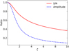 |
Fig. 1 Relation between the S/N or amplitude ratio and the DM mismatch factor ζ defined in Eq. (4). The solid red line represents the S/N relation, and the dashed blue line represents the amplitude relation. |
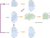 |
Fig. 2 Data-flow diagram for dedispersion, incorporating the stages of “write data,” “transpose,” “sub-band dedispersion,” and “shift data.” In this diagram, green memory blocks are used to buffer incoming data, and blue blocks serve as buffers for transposed data, where the dedispersion process takes place. The shaded patterns within the diagram illustrate the data mapping at various steps: (1) In the “write data” step, the shaded pattern represents the positions where the input data are written. (2) In the “transpose” step, the shaded pattern illustrates how the dedispersed data are transposed in buffers 1 and 2. (3) In the “sub-band dedispersion” step, the shaded pattern represents the dedispersion of the data. (4) In the “shift data” step, the shaded pattern illustrates the mapping of the data as they are shifted. |
2.4 Matched filtering
Following the dedispersion process, we obtain multiple time series corresponding to different DM trials. In accordance with the Neyman–Pearson lemma (Jerzy & Sharpe 1933), the most efficient test for two hypotheses involves employing the maximum likelihood ratio test. Consequently, we use the matched-filter algorithm to carry out pulse detection. To ensure efficiency in our implementation, we assumed that the pulse has a boxcar shape. We then applied a running boxcar window to the time series, calculating the S/N by
 (5)
(5)
where W represents the boxcar width, and t0 is the central time of the boxcar, Nbox is the number of samples within the boxcar, and σ is the standard deviation of the noise. The summation term in Eq. (5) can be computed in two steps: (1) Calculating the accumulation of the time series, and (2) subtracting the accumulation at the end sample and the start sample of the boxcar window. This computation has a complexity of 𝒪(N,) for one time series and one boxcar width. Under the assumption of Gaussian white noise, the probability of detection and false alarm for the statistics S/N can be expressed as
 (6)
(6)
 (7)
(7)
where y is the S/N threshold. Figure 4 displays the receiver-operating characteristic (ROC) curve. Given the unknown pulse width, we employed a running boxcar with various widths. We can deduce that the S/N decrease resulting from a mismatch in the boxcar width, denoted as ∆W, is
 (8)
(8)
S/Nopt represents the optimal S/N achieved with the optimal width. Figure 5 illustrates this relation. The extent of the S/N decrease relies on the ratio of the width mismatch and the true width. Hence, we used boxcar widths arranged in a geometric sequence with a tunable ratio to manage the S/N decrease in TRANSIENTX.
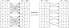 |
Fig. 3 Example sub-band dedispersion diagram with eight channels and DM trials. It presents the two stages of the sub-band dedispersion: (1) Dedispersing the data into sub-bands with a coarser DM grid. (2) Dedispersing the sub-banded data with a finer DM grid. |
2.5 Clustering
Following the pulse-detection process, we obtain an S/N cube that encompasses DM, time, and the width parameters. It is expected that when a pulse is located at a specific point within the S/N cube, we may observe neighboring regions around the true parameters where the S/N values exceed the detection threshold. This can lead to the generation of multiple duplicate candidates for a single pulse, which is undesirable. To address this issue and eliminate these duplicate candidates, we employed the density-based spatial clustering of applications with noise (DBSCAN) algorithm (Ester et al. 1996). To enhance its performance, we initially compressed the S/N cube into a two-dimensional DM-time plane. We achieved this by selecting the width with the highest S/N value for each DM and time combination. Additionally, we converted the DM dimension into dispersion delay using Eq. (1) to ensure that both dimensions share the same unit, such as milliseconds. Furthermore, we filtered out points with S/N values below the predefined S/N threshold.
In the DBSCAN algorithm, several key notations are used:
Core point: a point is considered a core point when it has a number of neighboring points that exceeds a predefined threshold k within a specified radius r.
Reachable point: a point is categorized as a reachable point when it is not a core point, but lies within the radius r of a core point.
Outlier: a point is classified as an outlier when it qualifies neither as a core point nor as a reachable point.
Density reachable: two points, denoted as p0 and pn, are regarded as density reachable when a chain of core points exists, including p1, p2,p3,…,pn−1, in which each adjacent point is within the radius r. Furthermore, both p0 and pn must be within the radius of p1 and pn_1 , respectively.
The algorithm can be summarized in the following steps: (1) Choosing an initial point p; (2) determining all density-reachable points with p that form one cluster when p is a core point; (3) choosing another point when p is not a core point; and (4) iterating through steps (1), (2), and (3) until all points have been processed.
In TRANSIENTX, we have developed an efficient C++ implementation of the DBSCAN algorithm. We leveraged a space-partitioning data structure called a kd-tree to divide the DM-time plane. This approach provides an efficient means to locate points within a given radius, with a complexity of 𝒪(log2 N). Figure 6 illustrates how the kd-tree partitions a two-dimensional plane. To find the neighboring points of a given point p0 within a radius r, the algorithm traverses the kd-tree. If the point p on a node falls within the radius r, it is marked as a neighboring point of p0, otherwise, it is not considered. To enhance the efficiency, branches can be eliminated from the traversal based on the following criteria: (1) When the point p on the node serves as a vertical divider, and the horizontal distance between p and p0 exceeds the radius r, then the branch in the opposite half of point p can be discarded. (2) When the point p on the node acts as a horizontal divider and the vertical distance between p and p0 surpasses the radius r, then the branch in the opposite half of point p can be omitted. This neighbor-point-finding algorithm greatly enhances the efficiency of the DBSCAN algorithm when applied in TRANSIENTX.
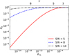 |
Fig. 4 ROC curve. The solid red, dashed blue, and dash-dotted black lines represent the ROC curve for pulses with S/N values of 5, 8, and 10, respectively, y is the S/N threshold. |
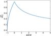 |
Fig. 5 Decrease in S/N as a function of the boxcar width mismatch. |
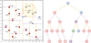 |
Fig. 6 Neighbor-finding algorithm using a kd-tree. The example demonstrates the process of finding neighboring points within a radius of r = 2 around a point (8, 9), denoted by a green circle. The left panel displays the plane divisions created by the points on the kd-tree. The dashed yellow and dotted purple lines divide the plane vertically and horizontally, respectively. The shaded yellow area represents the region within a radius of r = 2 from the point (8, 9). The right panel illustrates the kd-tree structure employed to identify neighboring points around the point (8, 9). The red circles indicate points that are not traversed, and the other circles represent points that are traversed. The purple points highlight the neighboring points found within the radius of r = 2. |
2.6 Candidate plotting
After the removal of duplicate candidates in the clustering process, a significant number of candidates still remains, including both genuine pulses and RFI signals. While machine-learning-based tools such as FETCH (Agarwal et al. 2020) can aid in the candidate classification, visual inspection remains a crucial step. To facilitate this, we generated figures for each candidate, incorporating essential meta-information such as DM, time of arrival, boxcar width, and the maximum Galactic DM contribution in the direction of the source, based on the YMW16 model (Yao et al. 2017). Additionally, each figure includes the dynamic spectra of the pulse and an S/N map in the DM-time plane, as exemplified in Fig. 7. To streamline the process of creating these candidate figures efficiently, we implemented a C++-based plotting library called PLOTX4. This library serves as a MATPLOTLIB-like wrapper for the high-performance plotting library PGPLOT5.
3 Benchmark
TRANSIENTX operates with a single command line, and the total elapsed time can vary even with the same configuration.
This variability arises because the clustering process depends on the number of clusters and the number of points within those clusters, which can differ significantly. To provide a clear understanding of the performance, we offer benchmarks for individual processes, encompassing dedispersion, matched filtering, and clustering: (1) For the dedispersion benchmark, we simulated datasets with varying numbers of frequency channels, resulting in different time costs. Additionally, we maintained the same number of DM trials as frequency channels. (2) For the matched-filtering benchmark, since the execution time scales linearly with the number of DMs, we provide time costs for different boxcar widths, offering insights into the impact of this parameter. (3) For the clustering benchmark, as TRANSIENTX processes data in small blocks with a duration of typically one second, we calculated the time costs for a single data block under different parameter configurations. Specifically, we varied the values of r and k in the DBSCAN algorithm. The data block contains a simulated single pulse, and we varied the number of points in a cluster by adjusting the S/N threshold.
For the benchmarking process, we used a simulated dataset with a time resolution of 153 µs and a length of 600 s. This configuration is similar to the MPIfR-MeerKAT Galactic Plane Survey of L-band (MMGPS-L; Padmanabh et al. 2023; Colora i Bernadich et al. 2023). The benchmark was conducted on a CPU model of Intel(R) Core(TM) i7-10750H. The results are presented in Fig. 8. From these results, several key observations can be made: (1) The time elapsed on the dedispersion process, which accounts for a significant portion of the total time, is shorter than the data length of 600 s even with 4096 frequency channels. This high efficiency demonstrates that TRANSIENTX can process large datasets. (2) The time elapsed on the matched-filter process scales linearly with the number of boxcar widths. This linear scalability arises because the computational complexity is 𝒪(Nt) and does not depend on the boxcar widths, as discussed in Sect. 2.4. (3) The time elapsed on the clustering process scales linearly with the total number of points to be clustered. Additionally, the clustering time increases with a larger radius r in the unit of samples due to additional iterations in traversing the kd-tree. For the entire single-pulse search process, TRANSIENTX demonstrates that it can process MMGPS data with 2048 frequency channels and a 153-microsecond time resolution in real time using a single CPU core. This shows its efficiency in processing demanding radio-astronomy datasets.
While our benchmark focused on MMGPS configuration test data, TRANSIENTX can be adapted to various data configurations, including low-frequency observations and microsecond timescales. In the pursuit of single-pulse detection in the lower radio frequency band (e.g., 100–200MHz), the dispersion delay can exceed 10 s. However, due to scattering effects that broaden the pulse, downsampling to lower time resolutions can reduce the requirements for memory and computation. Nevertheless, it is important to note that the sub-band dedispersion might slow down when the data within the sub-bands exceed the CPU L3-cache capacity. For microsecond-burst searches, it might be advantageous to adjust the data block length to fit the cache. In all cases, a proper DBSCAN parameter configuration based on the time resolution during the clustering process is vital to prevent slowdowns.
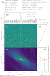 |
Fig. 7 Example candidate plot, created by TRANSIENTX. Panel a presents the essential meta-information about the pulse. Panel b displays the pulse profile. Panel c depicts the dynamic spectrum of the pulse. Panel d illustrates the S/N distribution in the DM-time plane after applying the matched filter. Panel e shows the pulse bandpass. Panel f shows the S/N vs. DM relation. The vertical solid red lines represent the S/N threshold, and the horizontal solid line denotes the measured DM of the pulse. The data path of the pulse are indicated along the right border. |
4 Discussions
CHIME/FRB Collaboration (2018) searched for the spectral index and scattering timescale in addition to DM, pulse width, and time of arrival. As a potential future improvement for TRANSIENTX, we investigated the S/N decrease caused by mismatches in spectral index and pulse shape.
4.1 Mismatch of the spectral index
In the dedispersion process, the frequency channels are typically combined with equal weights, although this may not represent the optimal weighting scheme. This is because real astronomical signals often exhibit nonflat spectra. For instance, pulsar signals frequently follow a power law with a negative index (Bates et al. 2013). Hence, the ideal approach involves a determination of the spectral index as well. The spectral data x with a spectral index α can be characterized as
 (9)
(9)
 (10)
(10)
 (11)
(11)
where fj represents the frequency in the jth channel, and σ represents the standard deviation of the noise. The S/N decrease resulting from a mismatch between the spectral index α and 0 can be expressed as
 (12)
(12)
 (13)
(13)
where ƒh and fl are the highest and lowest frequency, respectively. The S/N decrease caused by the mismatch of the spectral index for both ŋ = 2 and ŋ = 5 is depicted in the left panel of Fig. 9. The results show that for a typical pulsar spectral index of 2, the S/N decrease is only about 6% when ŋ = 2. However, FRB spectra can sometimes be narrowband (Kumar et al. 2021), leading to much larger S/N decreases, as seen in the case with a larger spectral index. Moreover, the S/N decrease becomes more pronounced as ŋ increases, particularly in the case of multi-octave receivers (e.g. Hobbs et al. 2020).
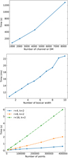 |
Fig. 8 Benchmark results for dedispersion, matched filtering, and clustering. The top panel depicts the relation between the dedispersion time cost and the number of frequency channels, which is equivalent to the number of DM trials. It demonstrates the efficiency of the dedispersion process. The middle panel shows the relation between the matched-filter time cost per DM trial and the number of boxcar widths. The linear scalability of the matched-filter process with respect to the number of boxcar widths is evident. The bottom panel illustrates how the clustering time scales with the number of points and is affected by the choice of radius, where the solid blue, dashed orange, and dash-dotted green lines represent a radius r 4, 8, and 16 in units of the samples, respectively. |
4.2 Mismatch of the pulse shape
In the matched-filter process, we employed a boxcar template. This may not represent the true pulse shape accurately and can result in S/N decrease. To quantify this S/N decrease, we derived a generalized S/N with a random pulse shape using the likelihood-ratio test,
 (14)
(14)
where s represents the pulse template. This equation reduces to Eq. (5) when the boxcar template is used. However, for the purpose of calculating the S/N decrease, we considered a Gaussian-shaped pulse template, s(t), with a scattering tail, given as
 (15)
(15)
where the asterisk represents the convolution, w and τS are the pulse width and scattering timescale, respectively. We then calculated the ratio of the S/N defined in Eqs. (5) and (14), and the results are shown in the right panel of Fig. 9. The S/N decrease caused by the mismatch of the pulse shape between a boxcar shape and a Gaussian shape with scattering is small, approximately 9%, even when the scattering timescale is ten times the pulse width.
5 Conclusions
We introduced a new high-performance single-pulse search software, TRANSIENTX, which is designed to be user-friendly and capable of running with a single command line while generating candidate figures. TRANSIENTX features an efficient CPU-based implementation of the sub-band dedispersion algorithm and an efficient implementation of the DBSCAN algorithm. These optimizations enable TRANSIENTX to provide efficient CPU-only real-time single-pulse searching capabilities. The application of TRANSIENTX in the Transients and Pulsars with MeerKAT (TRAPUM) project will be presented in future work (Carli et al., in prep.). Additionally, we conducted analyses to quantify the S/N decrease resulting from discrepancies in DM, pulse width, spectral index, and pulse shape. These investigations have improved our understanding of S/N decreases in single-pulse searches: (1) The S/N decrease due to the DM mismatch declines more slowly than the amplitude decrease. (2) The S/N decrease resulting from the spectral index mismatch becomes increasingly significant with multi-octave receivers. (3) The S/N decrease caused by the mismatch of the pulse shape between a boxcar and a Gaussian shape with scattering remains minor. It is worth noting that in a survey, the rate of the observed burst events might decline more rapidly than the decrease in S/N. This can be attributed to a steep S/N distribution, such as a power-law distribution with an index of -2, characterizing a uniform distribution of FRBs in the Universe. As we approach the era of the Square Kilometre Array (SKA), which will produce vast amounts of data, the need for real-time data-processing becomes increasingly critical. Advanced hardware and software solutions are essential to handle data volumes like this effectively. The experiments on TRANSIENTX and findings presented in this work can serve as valuable guidance for the development of future single-pulse search pipelines, especially for SKA data-processing.
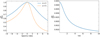 |
Fig. 9 Curves of the decrease in S/N. The left panel illustrates the S/N decrease with a mismatch in the spectral index when η = 2 and η = 5. The right panel depicts the S/N decrease with a mismatch in the pulse shape between a boxcar shape and a Gaussian shape with scattering. |
Acknowledgements
The MeerKAT telescope is operated by the South African Radio Astronomy Observatory, which is a facility of the National Research Foundation, an agency of the Department of Science and Innovation. SARAO acknowledges the ongoing advice and calibration of GPS systems by the National Metrology Institute of South Africa (NMISA) and the time space reference systems department of the Paris Observatory. TRAPUM observations used the FBFUSE and APSUSE computing clusters for data acquisition, storage and analysis. These clusters were funded and installed by the Max-PlanckInstitut für Radioastronomie and the Max-Planck-Gesellschaft. Y.P.M. and E.B. acknowledge continuing support from the Max Planck society.
Appendix A Decrease in S/N caused by a DM mismatch
For a radio pulse with a Gaussian profile, the dynamic spectrum is
 (A.1)
(A.1)
 (A.2)
(A.2)
 (A.3)
(A.3)
where w is the pulse width, and fc is the central frequency. By integrating x(f, t), we obtain the dedispersed profile,
 (A.4)
(A.4)
where ζ is defined in Equation (4). From Equation (5), we obtain
 (A.5)
(A.5)
where wm is the measured pulse width that gives the maximum S/N. Since wm cannot be derived analytically, we calculated it numerically. It is close to 2ζw as ζ becomes larger, as shown in Fig. A.1. For a given ζ, we then calculated the S/N decrease, as shown in Fig. 1.
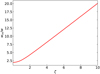 |
Fig. A.1 Optimal width relation with the DM mismatch factor ζ defined in Equation (4) that maximizes the measured S/N in the matched filter. |
References
- Agarwal, D., Aggarwal, K., Burke-Spolaor, S., Lorimer, D. R., & Garver-Daniels, N. 2020, MNRAS, 497, 1661 [Google Scholar]
- Barsdell, B. R., Bailes, M., Barnes, D. G., & Fluke, C. J. 2012, MNRAS, 422, 379 [CrossRef] [Google Scholar]
- Bates, S. D., Lorimer, D. R., & Verbiest, J. P. W. 2013, MNRAS, 431, 1352 [Google Scholar]
- CHIME/FRB Collaboration (Amiri, M., et al.) 2018, ApJ, 863, 48 [NASA ADS] [CrossRef] [Google Scholar]
- CHIME/FRB Collaboration (Amiri, M., et al.) 2021, ApJS, 257, 59 [NASA ADS] [CrossRef] [Google Scholar]
- Colom i Bernadich, M., Balakrishnan, V., Barr, E., et. al. 2023, A & A, 678, A187 [CrossRef] [EDP Sciences] [Google Scholar]
- Cordes, J. M., & McLaughlin, M. A. 2003, ApJ, 596, 1142 [NASA ADS] [CrossRef] [Google Scholar]
- Ester, M., Kriegel, H.-P., Sander, J., & Xu, X. 1996, in Proceedings of the Second International Conference on Knowledge Discovery and Data Mining, KDD'96 (AAAI Press), 226 [Google Scholar]
- Hewish, A., Bell, S. J., Pilkington, J. D. H., Scott, P. F., & Collins, R. A. 1968, Nature, 217, 709 [NASA ADS] [CrossRef] [Google Scholar]
- Hobbs, G., Manchester, R. N., Dunning, A., et. al. 2020, PASA, 37, e012 [NASA ADS] [CrossRef] [Google Scholar]
- Hurley-Walker, N., Rea, N., McSweeney, S. J., et. al. 2023, Nature, 619, 487 [NASA ADS] [CrossRef] [Google Scholar]
- Jerzy, N., & Sharpe, P. E. 1933, Philos. Trans. Roy. Soc. Lond. Ser. A, 231, 694 [Google Scholar]
- Keane, E. F. 2011, The Observatory, 131, 105 [NASA ADS] [Google Scholar]
- Kumar, P., Shannon, R. M., Flynn, C., et. al. 2021, MNRAS, 500, 2525 [Google Scholar]
- Large, M. I., Vaughan, A. E., & Wielebinski, R. 1968, Nature, 220, 753 [NASA ADS] [CrossRef] [Google Scholar]
- Magro, A., Karastergiou, A., Salvini, S., et. al. 2011, MNRAS, 417, 2642 [NASA ADS] [CrossRef] [Google Scholar]
- McLaughlin, M. A., Lyne, A. G., Lorimer, D. R., et. al. 2006, Nature, 439, 817 [NASA ADS] [CrossRef] [Google Scholar]
- Men, Y. P., Luo, R., Chen, M. Z., et. al. 2019, MNRAS, 488, 3957 [NASA ADS] [CrossRef] [Google Scholar]
- Men, Y., Barr, E., Clark, C. J., Carli, E., & Desvignes, G. 2023, A & A 679, A20 [NASA ADS] [CrossRef] [EDP Sciences] [Google Scholar]
- Morello, V., Rajwade, K. M., & Stappers, B. W. 2022, MNRAS, 510, 1393 [Google Scholar]
- Offringa, A. R., van de Gronde, J. J., & Roerdink, J. B. T. M. 2012, A & A, 539, A95 [NASA ADS] [CrossRef] [EDP Sciences] [Google Scholar]
- Padmanabh, P. V., Barr, E. D., Sridhar, S. S., et. al. 2023, MNRAS, 524, 1291 [NASA ADS] [CrossRef] [Google Scholar]
- Ransom, S. 2011, Astrophysics Source Code Library, [record ascl:1107.017] [Google Scholar]
- Snelders, M. P., Nimmo, K., Hessels, J. W. T., et. al. 2023, Nat. Astron., 7, 1486 [NASA ADS] [CrossRef] [Google Scholar]
- Taylor, J. H. 1974, A & AS, 15, 367 [NASA ADS] [Google Scholar]
- Yao, J. M., Manchester, R. N., & Wang, N. 2017, ApJ, 835, 29 [NASA ADS] [CrossRef] [Google Scholar]
- Zackay, B., & Ofek, E. O. 2017, ApJ, 835, 11 [NASA ADS] [CrossRef] [Google Scholar]
All Figures
|
Fig. 1 Relation between the S/N or amplitude ratio and the DM mismatch factor ζ defined in Eq. (4). The solid red line represents the S/N relation, and the dashed blue line represents the amplitude relation. |
| In the text | |
|
Fig. 2 Data-flow diagram for dedispersion, incorporating the stages of “write data,” “transpose,” “sub-band dedispersion,” and “shift data.” In this diagram, green memory blocks are used to buffer incoming data, and blue blocks serve as buffers for transposed data, where the dedispersion process takes place. The shaded patterns within the diagram illustrate the data mapping at various steps: (1) In the “write data” step, the shaded pattern represents the positions where the input data are written. (2) In the “transpose” step, the shaded pattern illustrates how the dedispersed data are transposed in buffers 1 and 2. (3) In the “sub-band dedispersion” step, the shaded pattern represents the dedispersion of the data. (4) In the “shift data” step, the shaded pattern illustrates the mapping of the data as they are shifted. |
| In the text | |
|
Fig. 3 Example sub-band dedispersion diagram with eight channels and DM trials. It presents the two stages of the sub-band dedispersion: (1) Dedispersing the data into sub-bands with a coarser DM grid. (2) Dedispersing the sub-banded data with a finer DM grid. |
| In the text | |
|
Fig. 4 ROC curve. The solid red, dashed blue, and dash-dotted black lines represent the ROC curve for pulses with S/N values of 5, 8, and 10, respectively, y is the S/N threshold. |
| In the text | |
|
Fig. 5 Decrease in S/N as a function of the boxcar width mismatch. |
| In the text | |
|
Fig. 6 Neighbor-finding algorithm using a kd-tree. The example demonstrates the process of finding neighboring points within a radius of r = 2 around a point (8, 9), denoted by a green circle. The left panel displays the plane divisions created by the points on the kd-tree. The dashed yellow and dotted purple lines divide the plane vertically and horizontally, respectively. The shaded yellow area represents the region within a radius of r = 2 from the point (8, 9). The right panel illustrates the kd-tree structure employed to identify neighboring points around the point (8, 9). The red circles indicate points that are not traversed, and the other circles represent points that are traversed. The purple points highlight the neighboring points found within the radius of r = 2. |
| In the text | |
|
Fig. 7 Example candidate plot, created by TRANSIENTX. Panel a presents the essential meta-information about the pulse. Panel b displays the pulse profile. Panel c depicts the dynamic spectrum of the pulse. Panel d illustrates the S/N distribution in the DM-time plane after applying the matched filter. Panel e shows the pulse bandpass. Panel f shows the S/N vs. DM relation. The vertical solid red lines represent the S/N threshold, and the horizontal solid line denotes the measured DM of the pulse. The data path of the pulse are indicated along the right border. |
| In the text | |
|
Fig. 8 Benchmark results for dedispersion, matched filtering, and clustering. The top panel depicts the relation between the dedispersion time cost and the number of frequency channels, which is equivalent to the number of DM trials. It demonstrates the efficiency of the dedispersion process. The middle panel shows the relation between the matched-filter time cost per DM trial and the number of boxcar widths. The linear scalability of the matched-filter process with respect to the number of boxcar widths is evident. The bottom panel illustrates how the clustering time scales with the number of points and is affected by the choice of radius, where the solid blue, dashed orange, and dash-dotted green lines represent a radius r 4, 8, and 16 in units of the samples, respectively. |
| In the text | |
|
Fig. 9 Curves of the decrease in S/N. The left panel illustrates the S/N decrease with a mismatch in the spectral index when η = 2 and η = 5. The right panel depicts the S/N decrease with a mismatch in the pulse shape between a boxcar shape and a Gaussian shape with scattering. |
| In the text | |
|
Fig. A.1 Optimal width relation with the DM mismatch factor ζ defined in Equation (4) that maximizes the measured S/N in the matched filter. |
| In the text | |
Current usage metrics show cumulative count of Article Views (full-text article views including HTML views, PDF and ePub downloads, according to the available data) and Abstracts Views on Vision4Press platform.
Data correspond to usage on the plateform after 2015. The current usage metrics is available 48-96 hours after online publication and is updated daily on week days.
Initial download of the metrics may take a while.