| Issue |
A&A
Volume 679, November 2023
|
|
|---|---|---|
| Article Number | A20 | |
| Number of page(s) | 10 | |
| Section | Numerical methods and codes | |
| DOI | https://doi.org/10.1051/0004-6361/202347356 | |
| Published online | 01 November 2023 | |
PulsarX: A new pulsar searching package
I. A high performance folding program for pulsar surveys
1
Max-Planck-Institut für Radioastronomie,
Auf dem Hügel 69,
53121
Bonn, Germany
e-mail: ypmen@mpifr-bonn.mpg.de
2
Max Planck Institute for Gravitational Physics (Albert Einstein Institute),
Callinstraße 38,
30167
Hannover, Germany
3
Leibniz Universität Hannover,
Welfengarten 1,
30167
Hannover, Germany
4
Jodrell Bank Centre for Astrophysics, Department of Physics and Astronomy, The University of Manchester,
Manchester
M13 9PL, UK
Received:
4
July
2023
Accepted:
5
September
2023
Context. Pulsar surveys with modern radio telescopes are becoming increasingly computationally demanding. This is particularly true for wide field-of-view pulsar surveys with radio interferometers and those conducted in real or quasi-real time. These demands result in data analysis bottlenecks that can limit the parameter space covered by the surveys and diminish their scientific return.
Aims. In this paper we address the computational challenge of ‘candidate folding’ in pulsar searching, presenting a novel, efficient approach designed to optimise the simultaneous folding of large numbers of pulsar candidates. We provide a complete folding pipeline appropriate for large-scale pulsar surveys that includes radio frequency interference mitigation, de-dispersion, folding, and parameter optimisation.
Methods. By leveraging the fast discrete dispersion measure transform (FDMT) algorithm, we have developed an optimised and cache-friendly implementation that we term the pruned FDMT (pFDMT). This implementation is specifically designed for candidate folding scenarios where the candidates are broadly distributed in dispersion measure space. The pFDMT approach efficiently reuses intermediate processing results and prunes the unused computation paths, resulting in a significant reduction in arithmetic operations. In addition, we propose a novel folding algorithm based on the Tikhonov-regularised least squares method that can improve the time resolution of the pulsar profile.
Results. We present the performance of its real-world application as an integral part of two major pulsar search projects conducted with the MeerKAT telescope: the MPIfR-MeerKAT Galactic Plane Survey (MMGPS) and the Transients and Pulsars with MeerKAT (TRAPUM) project. In our processing of approximately 500 candidates, the theoretical number of de-dispersion operations can be reduced by a factor of around 50 when compared to brute-force de-dispersion, which scales with the number of candidates.
Key words: methods: data analysis / pulsars: general
© The Authors 2023
 Open Access article, published by EDP Sciences, under the terms of the Creative Commons Attribution License (https://creativecommons.org/licenses/by/4.0), which permits unrestricted use, distribution, and reproduction in any medium, provided the original work is properly cited.
This article is published in open access under the Subscribe to Open model.
Open Access funding provided by Max Planck Society.
1 Introduction
Pulsars are compact stars that emit pulsed radiation at their rotational period (e.g. Hewish et al. 1968). The remarkable rotational stability of pulsars allows them to be treated as precise clocks, providing a natural tool for the measurement of astrophysical phenomena (e.g. Verbiest et al. 2008). Pulsars in binary systems can be used to test the limits of general relativity (e.g. Kramer et al. 2021) or the equation of state of supra-nuclear matter (e.g. Demorest et al. 2010; Antoniadis et al. 2013), while an array of pulsars distributed across the sky offers a natural detector for low-frequency gravitational waves (e.g. EPTA Collaboration and InPTA Collaboration 2023; Agazie et al. 2023; Reardon et al. 2023; Xu et al. 2023). Furthermore, in the case of radio pulsars, the broadband radio emission is altered by its propagation through the interstellar medium (ISM), allowing the inference of properties such as the Galactic free electron density (e.g. Cordes & Lazio 2002; Yao et al. 2017) and magnetic field (e.g. Han et al. 2018).
Since the discovery of the first pulsar (e.g. Hewish et al. 1968), more than 3000 sources have been discovered through pulsar searches, including Galactic plane and all-sky surveys (e.g. Large et al. 1968; Manchester et al. 1996; Cordes et al. 2006; Keith et al. 2010; Barr et al. 2013a; Stovall et al. 2014; Sanidas et al. 2019; Han et al. 2021; Padmanabh et al. 2023), globular clusters searches (e.g. Ransom et al. 2005; Hessels et al. 2007; Possenti et al. 2001; Pan et al. 2021; Ridolfi et al. 2021, 2022), and targeted observations of high-energy sources (e.g. Ransom et al. 2011; Cognard et al. 2011; Keith et al. 2011; Kerr et al. 2012; Camilo et al. 2015; Barr et al. 2013b; Cromartie et al. 2016; Wang et al. 2021; Bhattacharyya et al. 2021; Clark et al. 2023). In these surveys, SIGPROC (Lorimer 2011) and PRESTO (Ransom et al. 2002) have been two of the most popular software packages used for pulsar searching, both of which are CPU-based. The pulsar searching pipeline usually consists of several key stages: (1) Radio frequency interference (RFI) mitigation is performed to remove non-astrophysical signals from the raw data. (2) Dedispersion is performed to correct for the frequency-dependent delay caused by the propagation of the radio signal through the ISM. (3) Acceleration searching is performed to detect signals with periods that are changing as a function of time due to binary motion. (4) Finally, candidate folding is performed to extract the time- and frequency-resolved pulse profile of each detected signal. To improve performance, GPU-based software has also been developed to speed up the acceleration search (e.g. Allen et al. 2013; Dimoudi et al. 2018; Barr 2020), for example PEASOUP1. However, as presented in Lyon et al. (2016), the number of candidates produced by contemporary pulsar surveys is increasing, which is the result of improving survey technical specifications, such as time resolution and bandwidth. Furthermore, applying a signal-to-noise ratio (S/N) filter to limit the number of candidates is ineffective, and advanced candidate selection mechanisms, such as pulsar candidate classifiers, are required (e.g. Lee et al. 2013; Zhu et al. 2014; Balakrishnan et al. 2021). These classifiers work on post-folding data, which requires a larger number of candidates for folding initially. Therefore, a more efficient candidate folding process is helpful when dealing with the increasing number of candidates. In this work we have developed a new high performance folding program to address this performance issue; it is part of a new developing pulsar searching package, PULSARX2.
The algorithms used in our new folding program are presented in Sect. 2. We show the benchmarks in Sect. 3. The application of PULSARX to the MPIfR-MeerKAT Galactic Plane Survey in the L band (MMGPS-L; Padmanabh et al. 2023; Bernadich et al. 2023) is discussed in Sect. 4, and the conclusions are summarised in Sect. 5.
2 Algorithm
The purpose of the folding pipeline is to generate data cubes that can be used for visualisation or for classification by machine learning classifiers. Candidates from the acceleration search are parameterised by a spin frequency, v, a spin frequency derivative,  , and a dispersion measure (DM), as defined in Eq. (2). In the folding process, the time stamp, t, of each sample in the input time series is transformed to spin phase ϕ, which is predicted from ν and
  :
:
 (1)
(1)
where ϕ0 is the reference phase at t = 0. By integrating data samples over a discrete range of phase values, we obtain the signal power as a function of spin phase, otherwise known as the pulsar’s ‘profile’. To classify a candidate, it is useful to view the profiles in different frequency sub-bands and time sub-integrations. Therefore, we performed the folding process over discrete, contiguous ranges of time and frequency. The resulting collection of folded pulse profiles is referred to as an ‘archive’. The reference phase of all profiles in the archive can be adjusted to account for the difference between true and used values of DM, v and  of the candidate. The S/N of the candidate, summed over all profiles, will be maximised as these values approach their true values.
Because the raw data are often contaminated by RFI signals, it is necessary to perform RFI mitigation before the folding process. The data are then de-dispersed (see Sect. 2.2) into frequency sub-bands after RFI mitigation. These processes will be discussed in the following sections, and the data flow diagram is shown in Fig. 1.
2.1 RFI mitigation
Radio frequency interference signals are a common problem in radio observations. If not mitigated, RFI signals can significantly affect the profiles estimated during the folding process. Some algorithms have been widely used to mitigate the RFI signals (e.g. Offringa et al. 2012; Men et al. 2019; Morello et al. 2022). In our program, there are several RFI mitigation algorithms available, including the skewness-kurtosis filter (SKF), the zero-DM matched filter (ZDMF), and the Kadane filter (KF): (1) The SKF algorithm removes outliers based on the skewness and kurtosis of time samples in different frequency channels. (2) The ZDMF algorithm removes the correlated component between frequency channels in each channel, as discussed in Men et al. (2019). (3) The KF algorithm searches for the maximum summation along time samples in each frequency channel based on Kadane’s algorithm and replaces them by the mean value or a random value if the S/N is beyond a given threshold. Figure 2 shows an example of the SKF, ZDMF, and KF algorithms tested on observation data of MMGPS-L. Previous research has proposed using kurtosis-based RFI mitigation in baseband data (Nita et al. 2007). In the SKF, we extended this approach to filterbank data. Due to the presence of non-Gaussian noise in filterbank data, we adopted a threshold based on the inter-quartile range instead, which is similar to the inter-quartile range mitigation (IQRM) approach presented in Morello et al. (2022). The skewness and kurtosis definitions of SKF are shown in Appendix A, and the S/N definition of KF is shown in Appendix B.
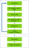 |
Fig. 1 Data flow of the candidate folding pipeline. The raw data are divided into blocks, and for each block the following steps are performed: RFI mitigation, normalisation, de-dispersion, and folding. Once all the data blocks have been folded, parameter optimisation and candidate plotting are carried out for each candidate. |
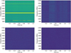 |
Fig. 2 Example of RFI mitigation with SKF, ZDMF, and KF. The test data used are from MMGPS-L and have 2048 frequency channels with a time resolution of 153 us. The SKF, ZDMF, and KF are applied successively to the raw data. The top-left panel displays the dynamic spectrum of the raw filterbank data. The top-right panel shows the dynamic spectrum of the data after application of the SKF, which removes the bad frequency channels. The bottom-left panel shows the dynamic spectrum of the data after application of the ZDMF, which eliminates zero-DM RFI signals and the baseline variation. Finally, the bottom-right panel shows the dynamic spectrum of the data after application of the KF, which removes long-duration RFI signals. |
2.2 De-dispersion
High frequency resolution is unnecessary for candidate classification. In addition, de-dispersing the data into sub-bands with low frequency resolution can accelerate the folding process by reducing the number of channels to be processed. As discussed in Sect. 3, de-dispersion becomes the bottleneck of the entire pipeline, and we adopted the fast discrete dispersion measure transform (FDMT) algorithm (Zackay & Ofek 2017) to speed up this process. However, the FDMT algorithm is designed for equally spaced DM trials, while candidate DMs are typically unevenly spaced. To address this, we modified the FDMT algorithm with a pruning strategy to accommodate the large, non-uniform DM trials encountered in de-dispersion. The modifications consist of three parts: (1) reordering the DM trials to enable in-place computation, which improves cache-friendliness; (2) pruning the unused intermediate de-dispersion computations; and (3) applying partial iterations of the FDMT algorithm to obtain the sub-band data. We refer to our modified algorithm as the pruned fast discrete dispersion measure transform (pFDMT). Since we were working with filterbank power data, we applied incoherent de-dispersion to correct for dispersion delays between frequency channels. The delay between frequencies f1 and f2 can be expressed as
 (2)
(2)
where e, me, and c are the elementary charge, electron mass, and speed of light in a vacuum, respectively.
The pFDMT algorithm consists of two steps: (1) generating the de-dispersion tree, which utilises the FDMT algorithm with a cache-friendly design that allows for in-place computation, and (2) pruning the tree to reduce the processing. To help explain the pFDMT algorithm, we first provide some definitions:
node: A time series of one frequency channel with a specific DM.
attribute: A parameter pair, consisting of a DM and channel index.
atomic de-dispersion: The process of de-dispersing two adjacent channels with one DM.
butterfly: A butterfly is composed of two consecutive atomic de-dispersions performed on adjacent channels with two successive DMs.
stage: Each stage consists of multiple butterflies.
root: A final de-dispersed time series with all frequency channels scrunched of a particular DM in the final stage.
In this paragraph, we describe the FDMT algorithm, while the modification will be described in the following paragraphs. The de-dispersion tree is composed of multiple stages, where each stage consists of multiple butterflies. In each stage, the butterflies perform de-dispersion on adjacent channels using a finer DM grid compared to the previous stage. This transformation results in new nodes with a DM step and a number of channels that are halved compared to the previous stage after each stage. Initially, the data consist of Nf frequency channels, at a single DM trial, for example DM = 0. In each step, pairs of neighbouring channels are de-dispersed at two DM trials spaced by half the total DM range, and summed together. After the nth stage, there are therefore Nf /2n sub-bands, de-dispersed at 2n DM values. As a result, the number of stages can be calculated as log2 Nf. In the first stage, each pre-transformed node’s attributes correspond to the channel index and the same DM of the starting DM trial. In the final stage, we obtain the de-dispersed time series of the DM trials.
To reduce the algorithm’s complexity, unused atomic de-dispersions can be pruned using the following steps: (1) starting from the nodes after the final stage and identifying the unused roots with DMs that are not among the candidate DMs; (2) pruning the atomic de-dispersions that lead to these roots; (3) moving to the previous stage and identifying nodes that do not have atomic de-dispersions to the pre-transformed nodes in the next stage; (4) pruning these atomic de-dispersions; and (5) repeating steps (3) and (4) until the first stage is reached.
To reduce the smearing caused by DM errors, we can adjust the DM step in the final stage of our algorithm. Furthermore, to improve the range of de-dispersed DMs, we can apply the pFDMT algorithm to multiple DM trials with different starting DM values. For larger DMs, intra-channel smearing becomes significant, and we can enhance computational efficiency by integrating samples to a coarser time resolution and increasing the DM step.
Since we only require the sub-band data and not the full de-dispersed time series, we can optimise the algorithm by stopping at the intermediate stage that corresponds to the desired number of frequency channels, denoted as Nsub. The computational operations of the pFDMT algorithm can be expressed as  , where Nt and Nf represent the number of time samples and frequency channels, respectively. The filling factor of all atomic de-dispersions, denoted by η, is dependent on the distribution of the DM trials. In contrast, the operations of performing brute-force de-dispersion for each candidate are NtNfNcand, where Ncand is the number of candidates. The computational operations are reduced by a factor of
  . The pseudo-code of the pFDMT algorithm is presented in Algorithm 1, and Fig. 3 illustrates an example with eight frequency channels. To execute the pFDMT algorithm in a CPU cache-friendly manner, we implemented a depth-first traversal recursive process, and the butterfly can be performed in place. Hence, the space complexity of the algorithm is 𝒪(NtNf).
2.3 Folding
To enhance the visual significance of the candidate’s profile and preserve its time variation information, we can perform intensity integration of the sub-banded data based on the spin phase over successive time spans. This process, known as folding, can be viewed as the estimation of the profile, s, of a periodic signal from the intensity time series, x. If we disregard the effects of sampling, we can model the intensity, x, as
 (3)
(3)
where ϕ(t) is the phase at time t that can be calculated from Eq. (1). n is the noise, which is assumed as Gaussian white noise with a mean of zero and a variance of σ2 in our calculation. The profile s can be approximated by a step function, given by
 (4)
(4)
 (5)
(5)
| 1: for i sub = 1, 2,…, nsub do |
| 2: DEDISPERSE(depthnsub, isub) |
| 3: end for |
| 4: procedure DEDISPERSE(depth, ichan) |
| 5: if depth == log2 Nf then |
| 6: D0,ichan = DM start |
| 7: return |
| 8: end if |
| 9: DEDISPERSE(depth+1,2*ichan) |
| 10: DEDISPERSE(depth+1, 2*ichan+1) |
| 11: for idm = 1,2,…, ndm do |
| 12: Didm,2*ichan+1 += DM step at current depth, i.e. 2depth times DM step at the root |
| 13: d0 = Didm,2*ichan |
| 14: d1 = Didm,2*ichan+1 |
| 15: BUTTERFLY(Xidm,2*ichan, Xidm,2*ichan+1, d0, d1) |
| 16: end for |
| 17: end procedure |
| 18: procedure BUTTERFLY(x, y, d0, d1) |
| 19: if path0 is activated then |
| 20: perform de-dispersion between x and y with DM = d0 |
| 21: update x with the de-dispersed time series above |
| 22: end if |
| 23: if path1 is activated then |
| 24: perform de-dispersion between x and y with DM = d1 |
| 25: update y with the de-dispersed time series above |
| 26: end if |
| 27: end procedure |
where k represents the kth phase bin of the profile; in other words, fk(ϕ) = 1 when the phase, ϕ, of a sample is located in the phase range of the kth phase bin. N represents the number of phase bins. ck is the coefficient of fk(ϕ), which can be estimated using the least squares method. χ2 is defined as
 (6)
(6)
where i represents the ith sample. It can be minimised to obtain the coefficients
 (7)
(7)
where Ck is the number of samples that locate in the kth phase bin. This is the algorithm used in the software package DSPSR (van Straten & Bailes 2011).
However, the time resolution of the profile estimated from this traditional folding algorithm is limited by the time resolution of the integrated samples in the raw data, as the integration effect introduced by sampling is not considered in Eq. (3). To address this issue, we propose a novel folding algorithm based on the Tikhonov-regularised least squares method (TRLSM), also known as ridge regression (Tikhonov 1943; Hoerl & Kennard 1970). We modified the signal model from Eq. (3), given by
 (8)
(8)
where Δt is the time resolution of one sample. Combined with Eq. (4) and Eq. (5), we have
 (9)
(9)
where wk(t) is the fraction of the kth phase bin swept by the sample at time t. Solving ck using the normal least squares method in Eq. (6) is an inverse problem that has a stability problem, which can be handled using the Tikhonov regularised χ′2:
 (10)
(10)
where λ is the ridge parameter (see Sect. 4.1 for a discussion of that). Equation (10) can be represented in the matrix form:
 (11)
(11)
where Τ represents the transposition. Minimising χ′2 gives
 (12)
(12)
where I is the identity matrix.
To investigate the performance of the TRLSM folding algorithm, we conducted a folding test on simulation data that include a periodic signal with Gaussian white noise. The signal has a Gaussian profile with a frequency of 650 Hz, and the data have a time resolution of 130 µs. Figure 4 illustrates the improvement of profile resolution achieved with the TRLSM folding algorithm compared to the DSPSR folding algorithm. Further investigation of this folding algorithm will be presented in future work (Men et al., in prep.).
In most real data folding cases, the time resolution is usually lower than or comparable to the phase resolution of the profile. Therefore, the weight matrix, W, is a sparse matrix, which significantly reduces the computing complexity of Eq. (12), namely,  , where Nn is the number of phase bins of the profile.
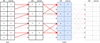 |
Fig. 3 Example of the pFDMT algorithm using eight frequency channels. The de-dispersion is only applied to DM = [1, 2], resulting in a de-dispersed sub-band data of two frequency channels. The output data are shaded in blue. The start DM is 0 and the DM step is 1, both of which can be adjusted. The solid red line indicates that the ‘atomic de-dispersion’ is non-pruned, while a translucent dashed black line or dotted red line indicate that it is pruned. The translucent dotted red line represents the pruned atomic de-dispersion in the final stage, which is not used as only sub-band data are needed. |
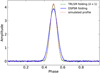 |
Fig. 4 Comparison between the TRLSM and DSPSR folding algorithms, using a folding example. The simulated profile is represented by a dotted red line, while the profile estimated from the DSPSR folding algorithm is shown as a solid blue line. The TRLSM folding algorithm is represented by a dashed green line, with a ridge parameter of λ = 1. |
2.4 DM, ν, and  optimisation
To find the optimal DM, v, and  parameters for each candidate, an additional optimisation step is required as the coarse grid of the parameter space in an acceleration search may not be optimal. We propose a novel iterative algorithm in our pipeline consisting of several steps in each iteration: (1) Calculate the integrated time-phase spectrum by scrunching the archive along all frequency channels. (2) Optimise v and
  by maximising the
  of the integrated profile, which is calculated by scrunching the time-phase spectrum along time. Here,
  , is defined as
 (13)
(13)
where  and
and  are the mean and variance of the noise inferred from the archive. (3) Correct the phase shifts of the profiles in the original archive with the updated ν and
  . (4) Calculate the integrated frequency-phase spectrum by scrunching the updated archive along time. (5) Optimise DM by maximising
  of the integrated profile, which is calculated by scrunching the frequency-phase spectrum along frequency. (6) Correct the phase shifts of the profiles in the updated archive with the updated DM. This iterative procedure terminates when the change of the parameters is less than a predefined precision. We used
  instead of S/N as the criterion for the significance of the profile because it can be efficiently computed. The complexity of this iterative optimisation algorithm is significantly lower than the brute-force algorithm that searches for the best DM, ν and
  in a three-dimensional grid.
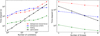 |
Fig. 5 Benchmark results of the folding pipeline, which includes de-dispersion, folding, and optimisation processes. The left panel illustrates the relation between time consumption and the number of candidates running on a single thread. The right panel shows the relation between time consumption and the number of threads with 512 candidates. The dotted red line represents the brute-force de-dispersion, while the dash-dot blue line represents the pFDMT algorithm. The folding process is represented by the dashed green line, and the optimisation process is represented by the solid black line. |
3 Benchmark
To evaluate the performance of our folding pipeline, we generated a simulated dataset with a similar format as the data in MMGPS-L, featuring a time resolution of 153 µs, 2048 frequency channels, and 10 min observation time. Rather than performing a full acceleration search, we instead simulated the input parameters of candidates for the folding pipeline. We used a logarithmic uniform distribution for the spin frequency ranging from 0.1 to 1000 Hz and a fixed zero value for the spin frequency derivative, which did not affect the folding and optimisation performance. We also used an equally spaced DM grid from 0 to 3000 cm−3 pc, which is the worst case for the pFDMT algorithm.
In PULSARX, there are two implementations of the folding pipelines: psrfold_fil and psrfold_fil2. The only difference between them is the de-dispersion algorithm they employ. The former utilises brute-force de-dispersion, while the latter utilises the pFDMT algorithm. We benchmarked the folding pipelines on a INTEL(R) XEON(R) SILVER 4116 CPU at 2.10 GHz, which is used in MMGPS-L. The results are presented in Fig. 5. From the left panel, we can see that the pFDMT algorithm becomes more efficient than the brute-force de-dispersion algorithm as the number of candidates increases, since the pFDMT algorithm has smaller memory input/output (IO) operations and computing complexity. The folding process consumes only about 10% of the time, which increases slowly in the regime of fewer candidates and becomes close to linearly scaled with more candidates. This is due to the fact that the memory I/O operations is reduced when there are more candidates since the folding process will reuse the sub-band de-dispersed data. This can also explain that the time consumption is not linearly scaled with the number of threads, as shown in the right panel of Fig. 5. The time consumption on the optimisation process is linearly scaled with the number of candidates as expected. It is expected that the optimisation process will dominate the time consumption when the number of candidates becomes larger. The right panel of Fig. 5 shows the scale relation of the time consumption with the number of threads, which is not linearly scaled except for the optimisation process, because the performance of the other processes are limited by memory I/O operations rather than computing power. In conclusion, psrfold_fil2 can operate almost in real-time with 8 CPU threads for about 500 candidates, which is highly efficient.
4 Discussions
4.1 The ridge parameter, λ
In the TRLSM folding algorithm, the ridge parameter, λ, is adjustable. Choosing a small value for λ can result in a noisy profile, while selecting a large value can lead to a broadening of the profile and reduced resolution. Finding the optimal ridge parameter for different regimes has been extensively studied (Ayinde & Lukman 2016). In our case, we can optimise λ to enhance the S/N of the profile. Here, we present a brief principle solution, and more details will be provided in future work (Men et al., in prep.). Firstly, we can demonstrate the algorithm within the Bayesian framework, where we interpret λ as the prior precision (i.e. the inverse variance) of the pulse profile amplitude for a single phase bin. In this framework, the likelihood and prior can be given as
 (14)
(14)
 (15)
(15)
respectively. We can then define the Bayes factor as
 (16)
(16)
By maximising K, which maximises the chi-square of the pulse profile, but with an ‘Occam’s razor’ penalty factor that prevents over-fitting (noisy pulse profiles) caused by a very small λ, we can obtain the optimal ridge parameter, λ.
4.2 Comparison with PRESTO
PRESTO3 is a widely used pulsar search package that offers various tools for different tasks, including rfifind for RFI mitigation, prepsubband for de-dispersion, prepfold for candidate folding, and so on. In this context, we provide a brief comparison between prepfold and psrfold_fil2, which both perform similar tasks, including RFI mitigation, de-dispersion, folding, and optimisation, but with different algorithms, prepfold performs these tasks for each candidate in a single run and employs a brute-force de-dispersion approach for each candidate. In the folding process, prepfold estimates the profile using с = WTx (i.e. λ = ∞ in Eq. (12); Bachetti et al. 2021). Additionally, prepfold applies brute-force optimisation in the three-dimensional grid of DM, v, and  . Furthermore, prepfold has the capability to fold intermediate products of de-dispersion in the searching stage, such as the de-dispersed time series or sub-band spectrum. It can perform the conversion of time from topocentric to barycentric reference frame, along with folding the binary candidate using the orbital parameters. These features are not currently supported in psrfold_fil2. However, efficient raw data folding can save the storage and disk I/O operations by eliminating the need for intermediate products of de-dispersion in the searching stage. To improve the efficiency of the folding pipeline, psrfold_fil2 applied several different algorithms, including (1) folding multiple candidates simultaneously to reduce the disk I/O operations; (2) using the pFDMT algorithm to speed up de-dispersion before folding when there are many candidates; (3) using a novel iterative optimisation algorithm to speed up the DM,v,
 optimisation significantly compared to the brute-force optimisation in a three-dimensional grid. We conducted a real benchmark comparison between the folding program in PULSARX and PRESTO, as depicted in Fig. 6. The results reveal that psrfold_fil2 outperforms prepfold by approximately 50 times when dealing with a large number of candidates. This benchmark employed an non-volatile memory express solid-state drive (NVMe SSD) with an I/O bandwidth of around 2 GB s−1. However, it is worth noting that prepfold demands significantly greater disk I/O operations, which implies that its performance will be notably slower when executed on a hard disk drive. These features make psrfold_fil2 particularly suitable for handling the folding processing of pulsar surveys with a large data rate, for example MMGPS and Transients and Pulsars with MeerKAT (TRAPUM).
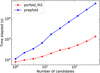 |
Fig. 6 Benchmark results obtained from a 10-min simulation dataset with 2048 frequency channels and a time resolution of 153 µs, comparing the folding program psrfold_fil2 in PULSARX with prepfold in PRESTO. The benchmark was conducted using an Intel(R) Core(TM) i7-10750H CPU clocked at 2.60 GHz, along with an NVMe SSD boasting a high bandwidth of approximately 2 GB s−1. |
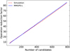 |
Fig. 7 Operation reduced factor achieved by the pFDMT algorithm compared to the brute-force algorithm. The solid blue line represents the test data obtained from MMGPS-L, where the number of candidates is determined based on the S/N cutoff. The dashed red line represents the simulated data with an equally spaced distribution of DMs. |
4.3 Application to the MMGPS-L
PULSARX has been employed within the MMGPS-L and TRAPUM projects. The TRAPUM initiative involves multiple sub-projects, including the Globular Cluster Survey, Fermi Source Survey, Nearby Galaxy Survey, and more, each characterised by distinct configurations. In this context, we focus on elucidating the specific application of PULSARX within the MMGPS-L project. The MMGPS-L is a wide field-of-view pulsar survey conducted with the MeerKAT telescope. Detailed information about the MMGPS-L configuration can be found in Padmanabh et al. (2023). This survey generates approximately 21 TB of data per hour, making it crucial to develop a highperformance processing pipeline capable of handling such a high data rate while working within the limitations of available disk space. For the acceleration search, we utilized the GPU-based acceleration search package PEASOUP and performed candidate folding using PULSARX. As PULSARX is CPU-based, it can run simultaneously with PEASOUP without resource competition. The time required for candidate folding in the MMGPS-L processing can be accommodated within the duration of the acceleration search. Figure 7 illustrates an example of the operation reduction factor achieved by the pFDMT algorithm using real DM trials of the candidates from a MMGPS-L observation. Notably, it is close to the equal-spaced DM trials. From the information presented in Fig. 7, it can be observed that the pFDMT algorithm achieves a significant operation reduction factor of approximately 50 when processing around 500 candidates. Figure 8 shows an example plot generated by the MMGPS-L processing pipeline.
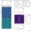 |
Fig. 8 Candidate plot generated by the folding pipeline of MMGPS-L, showing a known pulsar, PSR B1609-47. The plot is divided into eight panels: Panel a shows the folded profile of a candidate, with the grey vertical span indicating intra-channel dispersion smearing and red lines indicating pulse and noise amplitudes. Panel b shows the frequency-phase spectrum with time spans integrated. Panel c shows the time-phase spectrum with frequency channels integrated. Panel d shows the meta-information of the observation and candidate. Panel e shows the χ2-ν relation. Panel f shows the χ2 spectrum of the v- |


5 Conclusions
With the era of the Square Kilometer Array (SKA) approaching, more powerful computing hardware will be required to handle the massive amounts of data generated. Nonetheless, it is still worth exploring the more efficient algorithms that can significantly enhance the performance of the software we already use. This work introduces a new high performance folding program that includes an efficient de-dispersion algorithm and parameter optimisation, speeding up the pulsar searching pipeline significantly. Additionally, we have developed a skewness- and kurtosis-based RFI mitigation algorithm to remove the frequency channels contaminated by RFI signals. We propose a novel folding algorithm that can improve the resolution of the profile estimated from the folding process. We also demonstrate the application of the program to the MMGPS, showcasing its efficiency in handling the high data rate of this wide field-of-view interferometer-based pulsar survey. This provides inspiration for improving the performance of the pulsar searching pipeline in future radio telescopes, for example MeerKAT+ and SKA.
Acknowledgements
The authors would like to thank Scott Ransom for his helpful discussion regarding PRESTO. The MeerKAT telescope is operated by the South African Radio Astronomy Observatory, which is a facility of the National Research Foundation, an agency of the Department of Science and Innovation. SARAO acknowledges the ongoing advice and calibration of GPS systems by the National Metrology Institute of South Africa (NMISA) and the time space reference systems department of the Paris Observatory. TRAPUM observations used the FBFUSE and APSUSE computing clusters for data acquisition, storage and analysis. These clusters were funded and installed by the Max-Planck-Institut für Radioastronomie and the Max-Planck-Gesellschaft. E.C. acknowledges funding from the United Kingdom’s Research and Innovation Science and Technology Facilities Council (STFC) Doctoral Training Partnership, project reference 2487536. Y.P.M., E.B. and G.D. acknowledge continuing support from the Max Planck society.
Appendix A Skewness and kurtosis
The skewness, γ, and kurtosis, κ, of a time series are defined as
 (A.1)
(A.1)
 (A.2)
(A.2)
 (A.3)
(A.3)
respectively, where i represents the ith sample of the time series, and N is the number of total samples.
Appendix B S/N definition
After the KF has found the maximum summation in a time series x, the detection statistic S/N is defined as
 (B.1)
(B.1)
where a and b are the count of the start sample and end sample of the duration with maximum summation (i.e. a contiguous subarray in x with the largest sum), and σ is the standard deviation of the time series.
References
- Agazie, G., Anumarlapudi, A., Archibald, A. M., et al. 2023, ApJ, 951, L8 [NASA ADS] [CrossRef] [Google Scholar]
- Allen, B., Knispel, B., Cordes, J. M., et al. 2013, ApJ, 773, 91 [NASA ADS] [CrossRef] [Google Scholar]
- Antoniadis, J., Freire, P. C. C., Wex, N., et al. 2013, Science, 340, 448 [Google Scholar]
- Ayinde, K., & Lukman, A. 2016, Hacettepe J. Math. Stat., 46, 1 [Google Scholar]
- Bachetti, M., Pilia, M., Huppenkothen, D., et al. 2021, ApJ, 909, 33 [CrossRef] [Google Scholar]
- Balakrishnan, V., Champion, D., Barr, E., et al. 2021, MNRAS, 505, 1180 [NASA ADS] [CrossRef] [Google Scholar]
- Barr, E. 2020, Astrophysics Source Code Library [record ascl:2001.014] [Google Scholar]
- Barr, E. D., Champion, D. J., Kramer, M., et al. 2013a, MNRAS, 435, 2234 [NASA ADS] [CrossRef] [Google Scholar]
- Barr, E. D., Guillemot, L., Champion, D. J., et al. 2013b, MNRAS, 429, 1633 [Google Scholar]
- Bernadich, M. C.I., Balakrishnan, V., Barr, E., et al. 2023, arXiv e-prints [arXiv:2308.16802] [Google Scholar]
- Bhattacharyya, B., Roy, J., Johnson, T. J., et al. 2021, ApJ, 910, 160 [NASA ADS] [CrossRef] [Google Scholar]
- Camilo, F., Kerr, M., Ray, P. S., et al. 2015, ApJ, 810, 85 [NASA ADS] [CrossRef] [Google Scholar]
- Clark, C. J., Breton, R. P., Barr, E. D., et al. 2023, MNRAS, 519, 5590 [NASA ADS] [CrossRef] [Google Scholar]
- Cognard, I., Guillemot, L., Johnson, T. J., et al. 2011, ApJ, 732, 47 [NASA ADS] [CrossRef] [Google Scholar]
- Cordes, J. M., & Lazio, T. J. W. 2002, arXiv e-prints [arXiv:astro-ph/0207156] [Google Scholar]
- Cordes, J. M., Freire, P. C. C., Lorimer, D. R., et al. 2006, ApJ, 637, 446 [NASA ADS] [CrossRef] [Google Scholar]
- Cromartie, H. T., Camilo, F., Kerr, M., et al. 2016, ApJ, 819, 34 [Google Scholar]
- Demorest, P. B., Pennucci, T., Ransom, S. M., Roberts, M. S. E., & Hessels, J. W. T. 2010, Nature, 467, 1081 [Google Scholar]
- Dimoudi, S., Adamek, K., Thiagaraj, P., et al. 2018, ApJS, 239, 28 [NASA ADS] [CrossRef] [Google Scholar]
- EPTA Collaboration and InPTA Collaboration (Antoniadis, J., et al.) 2023, A&A, 678, A50 [CrossRef] [EDP Sciences] [Google Scholar]
- Han, J. L., Manchester, R. N., van Straten, W., & Demorest, P. 2018, ApJS, 234, 11 [NASA ADS] [CrossRef] [Google Scholar]
- Han, J. L., Wang, C., Wang, P. F., et al. 2021, Res. Astron. Astrophys., 21, 107 [CrossRef] [Google Scholar]
- Hessels, J. W. T., Ransom, S. M., Stairs, I. H., Kaspi, V. M., & Freire, P. C. C. 2007, ApJ, 670, 363 [NASA ADS] [CrossRef] [Google Scholar]
- Hewish, A., Bell, S. J., Pilkington, J. D. H., Scott, P. F., & Collins, R. A. 1968, Nature, 217, 709 [NASA ADS] [CrossRef] [Google Scholar]
- Hoerl, A. E., & Kennard, R. W. 1970, Technometrics, 12, 55 [Google Scholar]
- Keith, M. J., Jameson, A., van Straten, W., et al. 2010, MNRAS, 409, 619 [Google Scholar]
- Keith, M. J., Johnston, S., Ray, P. S., et al. 2011, MNRAS, 414, 1292 [NASA ADS] [CrossRef] [Google Scholar]
- Kerr, M., Camilo, F., Johnson, T. J., et al. 2012, ApJ, 748, L2 [NASA ADS] [CrossRef] [Google Scholar]
- Kramer, M., Stairs, I. H., Manchester, R. N., et al. 2021, Phys. Rev. X, 11, 041050 [NASA ADS] [Google Scholar]
- Large, M. I., Vaughan, A. E., & Wielebinski, R. 1968, Nature, 220, 753 [NASA ADS] [CrossRef] [Google Scholar]
- Lee, K. J., Stovall, K., Jenet, F. A., et al. 2013, MNRAS, 433, 688 [NASA ADS] [CrossRef] [Google Scholar]
- Lorimer, D. R. 2011, Astrophysics Source Code Library [record ascl:1107.016] [Google Scholar]
- Lyon, R. J., Stappers, B. W., Cooper, S., Brooke, J. M., & Knowles, J. D. 2016, MNRAS, 459, 1104 [NASA ADS] [CrossRef] [Google Scholar]
- Manchester, R. N., Lyne, A. G., D’Amico, N., et al. 1996, MNRAS, 279, 1235 [Google Scholar]
- Men, Y. P., Luo, R., Chen, M. Z., et al. 2019, MNRAS, 488, 3957 [NASA ADS] [CrossRef] [Google Scholar]
- Morello, V., Rajwade, K. M., & Stappers, B. W. 2022, MNRAS, 510, 1393 [Google Scholar]
- Nita, G. M., Gary, D. E., Liu, Z., Hurford, G. J., & White, S. M. 2007, PASP, 119, 805 [Google Scholar]
- Offringa, A. R., van de Gronde, J.J., & Roerdink, J.B.T.M. 2012, A&A, 539, A95 [NASA ADS] [CrossRef] [EDP Sciences] [Google Scholar]
- Padmanabh, P. V., Barr, E. D., Sridhar, S. S., et al. 2023, MNRAS, 524, 1291 [NASA ADS] [CrossRef] [Google Scholar]
- Pan, Z., Qian, L., Ma, X., et al. 2021, ApJ, 915, L28 [NASA ADS] [CrossRef] [Google Scholar]
- Possenti, A., D’Amico, N., Manchester, R.N., et al. 2001, arXiv e-prints [arXiv:astro-ph/0108343] [Google Scholar]
- Ransom, S. M., Eikenberry, S. S., & Middleditch, J. 2002, AJ, 124, 1788 [Google Scholar]
- Ransom, S., Hessels, J., Stairs, I., et al. 2005, ASP Conf. Ser., 328, 199 [NASA ADS] [Google Scholar]
- Ransom, S. M., Ray, P. S., Camilo, F., et al. 2011, ApJ, 727, L16 [NASA ADS] [CrossRef] [Google Scholar]
- Reardon, D. J., Zic, A., Shannon, R. M., et al. 2023, ApJ, 951, L6 [NASA ADS] [CrossRef] [Google Scholar]
- Ridolfi, A., Gautam, T., Freire, P. C. C., et al. 2021, MNRAS, 504, 1407 [NASA ADS] [CrossRef] [Google Scholar]
- Ridolfi, A., Freire, P. C. C., Gautam, T., et al. 2022, A&A, 664, A27 [NASA ADS] [CrossRef] [EDP Sciences] [Google Scholar]
- Sanidas, S., Cooper, S., Bassa, C. G., et al. 2019, A&A, 626, A104 [NASA ADS] [CrossRef] [EDP Sciences] [Google Scholar]
- Stovall, K., Lynch, R. S., Ransom, S. M., et al. 2014, ApJ, 791, 67 [CrossRef] [Google Scholar]
- Tikhonov, A. N. 1943, Proc. USSR Acad. Sci., 39, 195 [Google Scholar]
- van Straten, W., & Bailes, M. 2011, PASA, 28, 1 [Google Scholar]
- Verbiest, J. P. W., Bailes, M., van Straten, W., et al. 2008, ApJ, 679, 675 [NASA ADS] [CrossRef] [Google Scholar]
- Wang, P., Li, D., Clark, C. J., et al. 2021, Sci. China Phys. Mech. Astron., 64, 129562 [NASA ADS] [CrossRef] [Google Scholar]
- Xu, H., Chen, S., Guo, Y., et al. 2023, Res. Astron. Astrophys., 23, 075024 [CrossRef] [Google Scholar]
- Yao, J. M., Manchester, R. N., & Wang, N. 2017, ApJ, 835, 29 [NASA ADS] [CrossRef] [Google Scholar]
- Zackay, B., & Ofek, E. O. 2017, ApJ, 835, 11 [NASA ADS] [CrossRef] [Google Scholar]
- Zhu, W. W., Berndsen, A., Madsen, E. C., et al. 2014, ApJ, 781, 117 [NASA ADS] [CrossRef] [Google Scholar]
All Figures
|
Fig. 1 Data flow of the candidate folding pipeline. The raw data are divided into blocks, and for each block the following steps are performed: RFI mitigation, normalisation, de-dispersion, and folding. Once all the data blocks have been folded, parameter optimisation and candidate plotting are carried out for each candidate. |
| In the text | |
|
Fig. 2 Example of RFI mitigation with SKF, ZDMF, and KF. The test data used are from MMGPS-L and have 2048 frequency channels with a time resolution of 153 us. The SKF, ZDMF, and KF are applied successively to the raw data. The top-left panel displays the dynamic spectrum of the raw filterbank data. The top-right panel shows the dynamic spectrum of the data after application of the SKF, which removes the bad frequency channels. The bottom-left panel shows the dynamic spectrum of the data after application of the ZDMF, which eliminates zero-DM RFI signals and the baseline variation. Finally, the bottom-right panel shows the dynamic spectrum of the data after application of the KF, which removes long-duration RFI signals. |
| In the text | |
|
Fig. 3 Example of the pFDMT algorithm using eight frequency channels. The de-dispersion is only applied to DM = [1, 2], resulting in a de-dispersed sub-band data of two frequency channels. The output data are shaded in blue. The start DM is 0 and the DM step is 1, both of which can be adjusted. The solid red line indicates that the ‘atomic de-dispersion’ is non-pruned, while a translucent dashed black line or dotted red line indicate that it is pruned. The translucent dotted red line represents the pruned atomic de-dispersion in the final stage, which is not used as only sub-band data are needed. |
| In the text | |
|
Fig. 4 Comparison between the TRLSM and DSPSR folding algorithms, using a folding example. The simulated profile is represented by a dotted red line, while the profile estimated from the DSPSR folding algorithm is shown as a solid blue line. The TRLSM folding algorithm is represented by a dashed green line, with a ridge parameter of λ = 1. |
| In the text | |
|
Fig. 5 Benchmark results of the folding pipeline, which includes de-dispersion, folding, and optimisation processes. The left panel illustrates the relation between time consumption and the number of candidates running on a single thread. The right panel shows the relation between time consumption and the number of threads with 512 candidates. The dotted red line represents the brute-force de-dispersion, while the dash-dot blue line represents the pFDMT algorithm. The folding process is represented by the dashed green line, and the optimisation process is represented by the solid black line. |
| In the text | |
|
Fig. 6 Benchmark results obtained from a 10-min simulation dataset with 2048 frequency channels and a time resolution of 153 µs, comparing the folding program psrfold_fil2 in PULSARX with prepfold in PRESTO. The benchmark was conducted using an Intel(R) Core(TM) i7-10750H CPU clocked at 2.60 GHz, along with an NVMe SSD boasting a high bandwidth of approximately 2 GB s−1. |
| In the text | |
|
Fig. 7 Operation reduced factor achieved by the pFDMT algorithm compared to the brute-force algorithm. The solid blue line represents the test data obtained from MMGPS-L, where the number of candidates is determined based on the S/N cutoff. The dashed red line represents the simulated data with an equally spaced distribution of DMs. |
| In the text | |
|
Fig. 8 Candidate plot generated by the folding pipeline of MMGPS-L, showing a known pulsar, PSR B1609-47. The plot is divided into eight panels: Panel a shows the folded profile of a candidate, with the grey vertical span indicating intra-channel dispersion smearing and red lines indicating pulse and noise amplitudes. Panel b shows the frequency-phase spectrum with time spans integrated. Panel c shows the time-phase spectrum with frequency channels integrated. Panel d shows the meta-information of the observation and candidate. Panel e shows the χ2-ν relation. Panel f shows the χ2 spectrum of the v- |
| In the text | |
Current usage metrics show cumulative count of Article Views (full-text article views including HTML views, PDF and ePub downloads, according to the available data) and Abstracts Views on Vision4Press platform.
Data correspond to usage on the plateform after 2015. The current usage metrics is available 48-96 hours after online publication and is updated daily on week days.
Initial download of the metrics may take a while.