| Issue |
A&A
Volume 683, March 2024
|
|
|---|---|---|
| Article Number | A172 | |
| Number of page(s) | 14 | |
| Section | Extragalactic astronomy | |
| DOI | https://doi.org/10.1051/0004-6361/202348204 | |
| Published online | 18 March 2024 | |
The link among X-ray spectral properties, AGN structure, and the host galaxy
1
Instituto de Fisica de Cantabria (CSIC-Universidad de Cantabria), Avenida de los Castros, 39005 Santander, Spain
e-mail: gmountrichas@gmail.com
2
INAF – Osservatorio Astronomico di Roma, Via Frascati 33, 00040 Monteporzio Catone, Italy
3
Department of Physics, University of Helsinki, PO Box 64 00014 Helsinki, Finland
4
Jülich Supercomputing Centre, Forschungszentrum Jülich, Wilhelm-Johnen-Straße, 52428 Jülich, Germany
5
Institute of Astronomy, National Tsing Hua University, No. 101 Sect. 2 Kuang-Fu Road, 30013 Hsinchu, Taiwan
6
National Observatory of Athens, Institute for Astronomy, Astrophysics, Space Applications and Remote Sensing, Ioannou Metaxa and Vasileos Pavlou, 15236 Athens, Greece
Received:
9
October
2023
Accepted:
27
December
2023
In this work, we compare the supermassive black hole (SMBH) and host galaxy properties of X-ray obscured and unobscured AGN. For that purpose, we used ∼35 000 X-ray detected AGN in the 4XMM-DR11 catalogue for which there are available measurements for their X-ray spectral parameters, such as the hydrogen column density, NH, and photon index, Γ, from the XMM2Athena Horizon 2020 European project. We constructed the spectral energy distributions (SEDs) of the sources, and we calculated the host galaxy properties via SED fitting analysis, utilising the CIGALE code. We applied strict photometric requirements and quality selection criteria to include only sources with robust X-ray and SED fitting measurements. Our sample consists of 1443 AGN. In the first part of our analysis, we used different NH thresholds (1023 cm−2 or 1022 cm−2) while also taking into account the uncertainties associated with the NH measurements in order to classify these sources as obscured and unobscured (or mildly obscured). We find that obscured AGN tend to live in more massive systems (by ∼0.1 dex) that have a lower star-formation rate, SFR, (by ∼0.25 dex) compared to their unobscured counterparts. However, only the difference in stellar mass, M*, appears statistically significant (> 2σ). The results do not depend on the NH threshold used to classify AGN. The differences in M* and SFR are not statistically significant for luminous AGN (log (LX,2−10 KeV/erg s−1) > 44). Our findings also show that unobscured AGN have, on average, higher specific black hole accretion rates, λsBHAR, compared to their obscured counterparts, a parameter which is often used as a proxy of the Eddington ratio. In the second part of our analysis, we cross-matched the 1443 X-ray AGN with the SDSS DR16 quasar catalogue of Wu and Shen to obtain information on the SMBH properties of our sources. This resulted in 271 type 1 AGN at z < 1.9. Our findings show that type 1 AGN with increased NH (> 1022 cm−2) tend to have higher black hole masses, MBH, compared to AGN with lower NH values at similar M*. The MBH/M* ratio remains consistent for NH values below 1022 cm−2, but it exhibits signs of increasing at higher NH values. Finally, we detected a correlation between Γ and Eddington ratios, but only for type 1 sources with NH < 1022 cm−2.
Key words: methods: observational / galaxies: active / galaxies: evolution / galaxies: statistics / X-rays: galaxies / X-rays: general
© The Authors 2024
 Open Access article, published by EDP Sciences, under the terms of the Creative Commons Attribution License (https://creativecommons.org/licenses/by/4.0), which permits unrestricted use, distribution, and reproduction in any medium, provided the original work is properly cited.
This article is published in open access under the Subscribe to Open model. Subscribe to A&A to support open access publication.
1. Introduction
Active galactic nuclei (AGN) are powered by accretion onto the supermassive black hole (SMBH) that is located in the centre of most, if not all, galaxies. It is well known that AGN and their host galaxies co-evolve. This coeval growth is manifested in a number of ways. For instance, strong correlations have been found between the mass of the SMBH, MBH, and various galaxy properties, such as the bulge, or stellar mass (M*), and the stellar velocity dispersion of galaxies (e.g. Magorrian et al. 1998; Ferrarese & Merritt 2000; Häring & Rix 2004). Moreover, both the AGN activity and the star formation are fed by the same material (cold gas) and peak at similar cosmic times (z ∼ 2; e.g. Boyle et al. 2000; Sobral et al. 2013). Thus, for the purposes of understanding galaxy evolution, it is important to shed light on the structure of AGN in order to elucidate the physical mechanism(s) that feed the central SMBH and to study the AGN feedback.
One important aspect of this pursuit is to decipher the physical difference between obscured and unobscured AGN. According to the unification model (e.g. Urry & Padovani 1995; Nenkova et al. 2002; Netzer 2015), AGN are surrounded by a dusty gas torus structure that absorbs radiation emitted from the SMBH and the accretion disc around it. This absorbed radiation is then re-emitted at longer (infrared) wavelengths. In the context of this model, an AGN is classified as obscured or unobscured depending on the inclination of the line of sight with respect to the symmetry axis of the accretion disc and torus. When the AGN is observed edge-on, the source is characterised as obscured, while it is classified as unobscured when the AGN is viewed face-on. Recent investigations have proposed a more intricate structure for AGN to account for the diverse classifications observed at different wavelengths, such as X-ray versus optical classifications (e.g. Ogawa et al. 2021; Esparza-Arredondo et al. 2021). Advanced techniques such as infrared interferometry have enabled detailed examination of the inner regions of AGN, unveiling complexities within the torus and challenging the conventional notion of a simple, smooth toroidal model (e.g. Tristram et al. 2007). Studies focusing on short timescale variability in X-ray column density have identified fluctuations, indicating dynamic changes in the distribution of obscuring material (e.g. Marinucci et al. 2016). While the presence of clumps in the torus contributes to the diversity of observed AGN types and offers valuable insights into the accretion processes around SMBHs, according to the unification model, the inclination angle remains the pivotal factor for distinguishing between obscured and unobscured AGN.
An alternative interpretation of the AGN obscuration comes from the class of the evolutionary models. In this case, the different AGN types are attributed to SMBH and their host galaxies being observed at different phases. The main idea of these models is that obscured AGN are observed at an early phase, when the energetic output from the accretion disc around the SMBH is not strong enough and incapable of expelling the gas that surrounds it. As material is accreted onto the SMBH, its energetic output becomes more powerful and eventually pushes away the obscuring material (e.g. Ciotti & Ostriker 1997; Hopkins et al. 2006; Somerville et al. 2008).
Studying the two AGN populations can shed light on many different aspects of the AGN-galaxy interplay. An important step towards this direction is to first understand the nature of obscured and unobscured AGN. A popular approach to uncover their features and behaviours is to compare the host galaxy properties of the two AGN types. If the different AGN populations live in similar environments, this would provide support to the unification model, whereas if they reside in galaxies of different properties, it would suggest that they are observed at different evolutionary phases.
Previous studies that compared the host galaxy properties of obscured and unobscured AGN found conflicting results, depending on the wavelengths used to identify AGN (optical, infrared, X-rays) and the obscuration criteria applied to classify sources. For X-ray-selected AGN, when the source classification is based on optical criteria, for instance, using optical spectra to identify broad and narrow emission lines, most studies have found that obscured AGN (type 2) tend to live in more massive galaxies compared to their unobscured (type 1) counterparts. However, both AGN types live in systems with similar levels of star formation (e.g. Zou et al. 2019; Mountrichas et al. 2021a). When the classification is based on X-ray criteria, though, for instance on the value of the hydrogen column density, NH, some studies have not observed significant differences in the host galaxy properties of obscured and unobscured AGN (e.g. Masoura et al. 2021; Mountrichas et al. 2021c), while other studies have found an increase of M* with NH (Lanzuisi et al. 2017). Differences regarding both the M* and the stellar populations of the two AGN classes have also been reported (Georgantopoulos et al. 2023).
Another important aspect that can shed light on the structure of AGN is the study of the possible correlation between the X-ray spectral index, Γ, and the Eddington ratio, nEdd. The Eddington ratio is defined as the ratio of the AGN bolometric luminosity, Lbol, and the Eddington luminosity, LEdd (LEdd = 1.26 × 1038MBH/M⊙ erg s−1, where MBH is the mass of the SMBH). The relation between Γ and nEdd has been interpreted as the link between the accretion efficiency in the accretion disc and the physical status of the corona. Due to the larger amount of optical and UV photons produced by the accretion disc, the X-ray emitting plasma is more efficiently cooled at a higher nEdd (e.g. Vasudevan & Fabian 2007; Davis & Laor 2011). Alternatively, a correlation between Γ and nEdd could be explained by the significant dependence of the cut-off energy on the nEdd (for more details see Ricci et al. 2018). Apart from the physical interpretation of a possible correlation between Γ and nEdd, it is still not clear whether such a correlation is robust or universal, since relevant studies have found conflicting results (e.g. Shemmer et al. 2008; Risaliti et al. 2009; Sobolewska & Papadakis 2009; Brightman et al. 2013; Trakhtenbrot et al. 2017; Kamraj et al. 2022).
In this work, we utilised X-ray AGN from the 4XMM-DR11 catalogue, for which there are available measurements for their X-ray spectral parameters, within the framework of the XMM2Athena1 project. The 4XMM-DR11 dataset proved advantageous for our investigations due to its extensive collection of X-ray sources detected by the XMM-Newton observatory. The utilisation of XMM-Newton is particularly beneficial due to its high sensitivity and spatial resolution, allowing for the identification of faint and distant sources. Furthermore, the dataset demonstrates homogeneity, as the processed data within it adhere to a consistent processing methodology. Using the calculations for the spectral parameters, we classified sources into X-ray obscured and unobscured and compared their host galaxy properties. We then cross-matched the X-ray dataset with the Wu & Shen (2022) catalogue, which provides calculations for SMBH properties, such as black hole mass, MBH, and bolometric luminosity, Lbol, for SDSS quasars. This enabled us to compare the SMBH properties of the two AGN populations.
The paper is structured as follows. In Sect. 2, the two aforementioned catalogues are described. Section 3 presents the spectral energy distribution (SED) fitting analysis followed to measure the host galaxy properties. The selection criteria and the final samples are described in Sect. 4. Our results and conclusions are presented in Sect. 5. In Sect. 6, we summarise the main findings of this work.
2. Data
In this work, we used X-ray AGN included in the 4XMM-DR11 catalogue (Webb et al. 2020). The 4XMM-DR11 is the fourth generation catalogue of serendipitous X-ray sources from the European Space Agency’s (ESA) XMM-Newton observatory. It has been created by the XMM-Newton Survey Science Centre (SSC) on behalf of ESA. The catalogue contains 319 565 detections with spectra in 11 907 observations. There are 100 237 (31.4%) detections that were made in both detectors, 135 342 (45.5%) detections that come solely from the pn detector, and 73 986 (23.2%) detections that are only from the MOS cameras.
There are 210 444 sources that have available spectrum from one or more detections. The process followed for the classification and fitting of these sources has been done within the framework of the XMM2Athena project and is described in detail in Viitanen et al. (in prep.). In brief, the Tranin et al. (2022) catalogue was used to classify the sources. In Tranin et al. (2022), they used a reference sample constructed by cross-matching the Swift-XRT (2SXPS; Evans et al. 2020) sample and the tenth data release of the XMM-Newton serendipitous dataset (4XMM-DR10) with catalogues of identified AGN, stars, and other X-ray source types (for more details, see their Table 2 and Sect. 2.1.2). The 210 444 sources were cross-matched with the Tranin et al. (2022) catalogue using a matching radius of 1″. The final number of sources with available classification is 92 238. Out of them, 76 610 are AGN, 14 308 are stars, 1091 are X-ray binaries (XRBs), and 229 are cataclysmic variables (CVs).
For the X-ray sources classified as AGN, we calculated photometric redshifts for those with a reliable optical counterpart in SDSS or PanSTARRS following the methodology presented in Ruiz et al. (2018). In the case of SDSS sources with spectroscopic observations, the corresponding redshift was used instead. There are 35 538 AGN with available redshift (8467 of them have spectroscopic redshift). A detailed presentation of this photometric redshift catalogue is presented in Ruiz et al. (in prep.).
The X-ray spectral analysis of these AGN was conducted within the framework of the XMM2Athena project (Webb et al. 2023). Details of this analysis can be found in Viitanen et al. (in prep.). In summary, a Bayesian spectral fit is performed with the BXA tool (Buchner et al. 2014) that facilitates the connection between XSPEC, which is used for the analysis of the X-ray spectral data (Arnaud 1996), and the nested sampling package UltraNest (Buchner et al. 2021). An uninformative prior was assigned to each parameter within the model, and the exploration of the entire parameter space with equal-weighted sampling points was carried out using the MLFriends algorithm (Buchner 2019), implemented within UltraNest. UltraNest is a Bayesian inference library designed for high-dimensional parameter estimation and model selection. UltraNest employs a nested sampling algorithm that works by enclosing high likelihood regions within a set of nested iso-likelihood contours. The algorithm then successively samples from the prior within these contours, effectively exploring the parameter space in a way that efficiently allocates computational resources to regions of higher likelihood. This makes nested sampling particularly effective for problems with multiple modes, as it naturally discovers and characterises these modes. As part of the fitting process, the empirical background model in the BXA.SHERPA.BACKGROUND module was utilised. This model has two parts. One part models the detector background and contains the contribution of lines and is not folded through the instrumental response. The second part accounts for emission of the cosmic X-ray background and X-ray emission of the local hot bubble and Galactic halo. The background model, which is made up of a mixture of power laws, Gaussian lines, and thermal emission components, is fitted in a multi-step process to the background spectrum with the model increasing in complexity in each step and with the parameters of the previous steps constrained within a narrow range of the best-fit value obtained in the previous step. An χ2 test was used to estimate the goodness of fit of the background spectra, and p-values were then obtained based on the χ2 values and the number of effective parameters.
For the fitting of the source X-ray spectrum, a power law with two absorbing media was used: the local Galactic absorption with the column density fixed to the total column density in that line of sight plus in situ absorption at the AGN redshift with a free column density. For the free parameters of the model, the following priors were applied: log fX ∈ −17, −7 (erg s−1 cm−2);Γ ∈ 0, 6, log NH ∈ 20, 26 (cm−2);and IIN (normalisation)∈0, 5, where fX and IIN are the X-ray flux and the inter-instrument normalisation (in the case of PN and MOS detections). To quantify the goodness of fit, a p-value is provided in the catalogue. Its calculation is described in detail in Viitanen et al. (in prep.). For each free parameter the catalogue includes the median and mode values, the 5 and 95 percentiles as well as the values that encompass the narrowest 90% interval (taken as the uncertainty of the mode). The parameters used in our analysis are the mode values of NH, Γ, and the fluxes (calculated in the 2–10 keV energy band). Using these estimated parameters, the X-ray luminosities, LX, were calculated after correcting for the fitted intrinsic absorption. We opted for mode values because they are the most probable values of the distribution, and they capture the cases that are closer to the edges of the sampled interval better than the median values. It is important to highlight that this selection, however, does not impact the overall results and conclusions of our study. An example of a source spectrum and model fit including the background modelling is presented in Fig. 1.
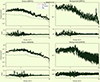 |
Fig. 1. Example of a source spectrum and model fit (left panels), including the background modelling (right panels) for the PN (top panels) and MOS (bottom panels). |
One goal of this study is to compare the SMBH properties of X-ray obscured and unobscured AGN. To add this information to our sources, we cross-matched the 35 538 AGN with the Wu & Shen (2022) catalogue. This catalogue includes the continuum and emission line properties for 750 414 broad-line quasars from the data release 16 of SDSS (DR16Q) measured through optical spectroscopy. The quasars span a range of 0.1 ≤ z ≤ 6 and 44 ≤ log (Lbol/erg s−1) ≤ 48, and the Lbol were calculated using the measured continuum luminosity at rest-frame wavelengths of 5100 Å, 3000 Å and 1350 Å, depending on the redshift of the source (for more details see Sect. 4.1 in Wu & Shen 2022). The catalogue also includes single-epoch virial MBH. The MBH have been calculated adopting the fiducial recipes on H β (for sources with z < 0.7) or the Mg II (for sources with 0.7 ≤ z < 1.9) lines. At higher redshifts, the C IV line was measured. These MBH and Lbol were used to calculate the nEdd.
The default redshifts in DR16Q are mostly based on the redshifts derived by the SDSS pipeline (Bolton et al. 2012). Lyke et al. (2020) also visually inspected a small fraction of quasars and updated their default redshift in DR16Q with visual redshifts. In the catalogue provided by Wu & Shen (2022), they presented improved systemic redshifts using the measured line peaks and correcting for velocity shifts of various lines with respect to the systemic velocity (for more details, see their Sect. 4.2).
3. Calculation of the host galaxy properties
For the calculation of the star-formation rate, SFR, and stellar mass, M*, of the AGN host galaxies, we applied SED fitting using the CIGALE algorithm (Boquien et al. 2019; Yang et al. 2020, 2022). CIGALE allows for the inclusion of the X-ray flux in the fitting process and has the ability to account for the extinction of the UV and optical emission in the poles of AGN (Yang et al. 2020; Mountrichas et al. 2021b,a; Buat et al. 2021).
We used the same templates and parametric grid in the SED fitting process as those used in recent works (Mountrichas et al. 2021c, 2022c,a, 2023; Mountrichas & Shankar 2023). In brief, the galaxy component was modelled using a delayed star-formation history, SFH, model with a function form SFR ∝ t × exp(−t/τ). A star formation burst was included (Małek et al. 2018; Buat et al. 2019) as a constant ongoing period of star formation of 50 Myr. Stellar emission was modelled using the single stellar population templates of Bruzual & Charlot (2003) and was attenuated following the Charlot & Fall (2000) attenuation law. To model the nebular emission, CIGALE adopts the nebular templates based on Villa-Velez et al. (2021). The emission of the dust heated by stars was modelled based on Dale et al. (2014), without any AGN contribution. The AGN emission was included using the SKIRTOR models of Stalevski et al. (2012, 2016). CIGALE has the ability to model the X-ray emission of galaxies. In the SED fitting process, the intrinsic LX in the 2 − 10 keV band were used. The parameter space used in the SED fitting process is shown in Table 1.
Models and the values for their free parameters used by CIGALE for the SED fitting.
4. Selection criteria and final samples
From the 35 538 AGN available in our catalogue, we used those with flag = 0, provided by the catalogue produced by the XMM2Athena. A detailed description of the flag numbering is given in Viitanen et al. (in prep.). In brief, sources with flag = 0 have background and source fits with a p-value > 0.01, which is the threshold used to classify a fit as acceptable. There were 29 509 AGN that met this criterion. In our analysis, we needed reliable estimates of the host galaxy properties via SED fitting measurements. Therefore, we required all our X-ray AGN to have available photometry from SDSS or Pan-STARRS, 2MASS, and WISE in the following bands: (u),g, r, i, z, (y),J, H, K, W1, W2, and W4 (e.g. Mountrichas et al. 2021a,c, 2022c,a; Buat et al. 2021). There were 2,501 AGN that fulfilled these requirements. We note that, although we did not require it, all of these AGN also have W3 measurements available. For these sources, we applied an SED fitting using the templates and parameter space described in Sect. 3.
To restrict our analysis of sources to those with the most reliable host galaxy measurements, we excluded badly fitted SEDs. For that purpose, we considered only sources for which the reduced χ2,  . This value has been used in previous studies (e.g. Masoura et al. 2018; Buat et al. 2021; Mountrichas et al. 2022c,a; Koutoulidis et al. 2022; Pouliasis et al. 2022) and is based on visual inspection of the SEDs. This requirement was met by 78% of the sources. To further exclude systems with unreliable measurements of the host galaxy properties, we applied the same method presented in previous studies (e.g. Mountrichas et al. 2021c,a, 2023; Buat et al. 2021; Koutoulidis et al. 2022). This method is based on a comparison between the value of the best model and the likelihood-weighted mean value calculated by CIGALE. Specifically in our analysis, we only considered sources with
  and
and  , where SFRbest and M*, best are the best-fit values of SFR and M*, respectively, and SFRbayes and M*, bayes are the Bayesian values estimated by CIGALE. The SFR and M* criteria were met by 88% and 97% of the sources. Previous studies have employed these ranges for the selection of reliable SFR and M* estimations while leveraging the CIGALE code (e.g. Mountrichas et al. 2021a,c, 2022c,a,b, 2023; Mountrichas & Shankar 2023; Buat et al. 2021; Koutoulidis et al. 2022; Pouliasis et al. 2022). Mountrichas et al. (2021c) explored variations in the range, considering 0.1 − 0.33 for the lower limit and 3 − 10 for the upper limit. They affirmed that the outcomes remained insensitive to the specific choice of these limits. In our study, we validate this observation by investigating the impact of varying these boundaries within the specified limits. Our findings indicate that such variations result in a dataset size change of less than 5%, underscoring that they do not introduce significant alterations to our overall results and conclusions.
We also restricted the sample used in our analysis to sources with z < 1.9. The reason is twofold: our dataset does not include obscured sources at higher redshifts, and MBH measurements available in the Wu & Shen (2022) catalogue are not reliable at z > 1.9 (i.e. MBH calculated using the C IV broad line are considered less reliable). Finally, we excluded sources for which their redshift in the XMM dataset differs more than 0.1 compared to the redshift quoted in the Wu & Shen (2022) catalogue (16 AGN were excluded from this criterion). This threshold was determined by considering that during the process of SED fitting, redshift values are rounded to the nearest tenth decimal place. We note that no filtering has been applied regarding the uncertainties associated with the photometric redshifts available in our catalogue. The vast majority of sources with erroneous photometric redshifts would result in poor SED fits and consequently be excluded by the SED quality criteria previously described. Furthermore, we conducted an investigation to determine whether our results were impacted when restricting the analysis solely to AGN with spectroscopic redshifts, which is discussed in the following section.
There were 1443 X-ray AGN that fulfilled these criteria. Of these sources, 1231 lie at z < 0.7 and 212 at 0.7 ≤ z < 1.9. This sample was used in the analysis presented in Sects. 5.1 and 5.2. Of the 1443 AGN, 344 are also included in the Wu & Shen (2022) catalogue. Out of them, 271 are at z < 1.9. These 271 AGN were used in our analysis presented in Sect. 5.3.
5. Results and discussion
In this section, we compare the properties of host galaxies (SFR, M*) and SMBHs (nEdd) X-ray obscured and unobscured AGN. We also study the Lbol − MBH and MBH −M* relations as a function of X-ray obscuration (NH). Finally, we investigate the relation between the powerlaw slope (Γ) of the X-ray spectral model with nEdd.
5.1. Host galaxy properties of X-ray obscured and unobscured active galactic nuclei
In our analysis, we used the 1 443 AGN that met the criteria described in Sect. 4. Their distribution in the LX-redshift plane is presented in Fig. 2. We first split the sources into X-ray obscured and unobscured (or mildly obscured) AGN using an NH limit of 1023 cm−2. Specifically, we used the lower and upper limits of the 90% confidence interval on the NH mode from the spectral fitting analysis. An AGN was classified as obscured if the lower limit of their NH value was higher than 1023 cm−2. Similarly, an AGN was identified as unobscured (or moderately obscured) if the upper limit of its NH value was lower than 1023 cm−2. Table 2 presents the number of sources classified. Then, we compared the SFR and M* of the host galaxies of the two AGN populations. The selection of classification criteria served a dual purpose. Firstly, it relied on recent research findings (Georgantopoulos et al. 2023) that highlight that distinctions in the properties of SMBHs and their host galaxies between obscured and unobscured AGN tend to diminish when the NH value falls below the threshold of NH < 23 cm−2. Secondly, by taking into account the uncertainties associated with NH, the classification ensured that only firmly obscured and unobscured sources were categorised as such, enhancing the reliability of the classification process.
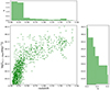 |
Fig. 2. Distribution of the 1443 X-ray AGN in the LX-redshift plane. |
Weighted median values of SFR, M*, and λsBHAR for obscured and unobscured AGN.
The results are presented in Fig. 3. In the figure, we have restricted both datasets to z < 0.7. This is because there are no AGN classified as obscured using the criteria described above, at z > 0.7, in our dataset. We also note that the distributions have been weighted to account for the different LX and redshift of obscured and unobscured AGN. For that purpose, each source was assigned a weight based on its LX and redshift following the procedure described in Mountrichas et al. (2019, 2021c, 2022b), Masoura et al. (2021), Buat et al. (2021), Koutoulidis et al. (2022). Specifically, the weight was calculated by measuring the joint LX distributions of the two populations (i.e. we added the number of obscured and unobscured AGN in each LX bin in bins of 0.1 dex) and then normalising the LX distributions by the total number of sources in each bin. The same procedure was followed for the redshift distributions. The total weight that was assigned in each source was the product of the two weights. We made use of these weights in all distributions presented in the remainder of this section.
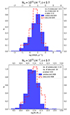 |
Fig. 3. Host galaxy properties of X-ray obscured (red dashed line histograms) and unobscured AGN (blue shaded histograms). Sources are classified as obscured when the lower limit of their NH value is higher than 1023 cm−2. We classified AGN as unobscured if the upper limit of their NH value is below 1023 cm−2. The top panel presents the SFR distributions of the two AGN populations. The bottom panel shows their M* distributions. The number of sources and the p-values obtained by applying a KS test are shown in the legend of the plots. Distributions are weighted based on the redshift and LX of the sources. |
Figure 3 shows the distributions of unobscured (blue shaded histograms) and obscured AGN (red dashed line histograms). The top panel presents the SFR distributions of the two AGN classes. The (weighted) median log SFR of the unobscured and obscured AGN is 0.82 and 0.57, respectively (Table 2). Applying a Kolmogorov-Smirnov (KS) test yielded a p-value of 0.10 (also shown in the legend of the plot). Similar p-value were obtained by applying a Mann-Whitney test (MW; p-value = 0.14) and a Kuiper (p-value = 0.32) test. Therefore, the difference of 0.25 dex does not appear statistically significant (two distributions differ with a statistical significance of ∼2σ for a p-value of 0.05).
The bottom panel of Fig. 3 shows the M* distributions of obscured (blue shaded histogram) and unobscured (red dashed line) AGN. The weighted median of the log M* is 10.86 and 10.95 for unobscured and obscured AGN, respectively. Although the difference is small, it appears to be statistically significant (Table 2). Specifically, the p-value derived from the KS test was 0.02. Similar p-value were also obtained by applying MW and Kuiper tests (< 0.05). We note that the (weighted) standard deviations (SDs) of the two populations are 11.22 (obscured) and 11.13 (unobscured). The (weighted) 95% confidence intervals (CI) are 10.91 − 11.30 and 10.99 − 11.07 for the obscured and unobscured AGN, respectively. Therefore, based on our results, obscured AGN tend to live in more massive systems, and their hosts have a lower SFR compared to their unobscured counterparts. However, only the M* difference appears to be statistically significant.
Furthermore, we explored whether our outcomes are influenced by potential redshift evolution within the z < 0.7 redshift range encompassed by our dataset. For that purpose, we split the AGN sample into two redshift bins using the median value of the z < 0.7 dataset (i.e. at z = 0.21). The results do not appear redshift dependent since similar trends and p-values were obtained. Additionally, we examined whether our findings might be sensitive to uncertainties associated with photometric redshift estimates. To address this concern, we narrowed down our analysis to include only sources with spectroscopic redshifts. We obtained similar results in this restricted subset.
Most previous studies that examined the host galaxy properties of X-ray obscured and unobscured AGN did not find (significant) differences for the SFR and M* of the hosts of the two AGN populations. Specifically, Masoura et al. (2021) and Mountrichas et al. (2021c) studied the SFR and M* of X-ray obscured and unobscured AGN at 0 < z < 3.5 using data from the XMM-XXL and the Boötes fields, respectively, and concluded that both AGN classes live in galaxies with similar properties (see also Merloni et al. 2014). We note that the aforementioned studies did not account for the uncertainties in the NH values and applied a lower NH threshold (NH = 1021.5 cm−2) to classify their AGN. However, Lanzuisi et al. (2017) studied AGN at 0.1 < z < 4 in the COSMOS field and found that the average NH shows a clear positive correlation with M* but not with the SFR. Studies that used optical criteria (e.g. optical spectra) to classify the AGN into type 1 and type 2 found that the two AGN types live in galaxies with similar SFR, but type 2 sources tend to reside in more massive systems, by ∼0.3 dex, both at low redshift (z < 1; Mountrichas et al. 2021c) and at high redshift (z < 3.5; Zou et al. 2019).
More recently, Georgantopoulos et al. (2023) compared the stellar populations and M*, among others, of X-ray obscured and unobscured AGN host galaxies in the COSMOS field at z ∼ 1 using NH = 1023 cm−2 to classify their sources. Their analysis showed that the distribution of M* of obscured AGN is skewed to a higher M* compared to unobscured AGN. Specifically, they found that heavily obscured AGN live in galaxies that have a higher M* by 0.13 dex compared to unobscured sources. Although the difference was small, it was statistically significant (p-value = 1.3 × 10⁻³). Notably, their results are in excellent agreement with our findings. They also found that heavily obscured AGN tend to live in systems with older stars compared to unobscured AGN. This is consistent with our finding of a lower SFR for heavily obscured AGN hosts compared to those that are unobscured, although in our measurements the difference did not appear statistically significant.
Georgantopoulos et al. (2023) suggested that a possible cause for the discrepant results among previous studies could be the different NH thresholds that were used. Indeed, when they lowered the NH value used to classify their AGN, the statistical significance of the differences detected in the host galaxy properties of the two AGN classes was lower (see their Fig. 13). To verify this hypothesis, we lowered the NH threshold utilised for our AGN classification to NH = 1022 cm−2 using the lower and upper limits of NH specified at the outset of this section and repeated the analysis. The findings are showcased in Fig. 4 and Table 2. Results similar to those presented in Fig. 3 emerged. Specifically, obscured AGN tend to inhabit more massive systems (by 0.12 dex) and have a lower SFR (by 0.26 dex) compared to unobscured AGN. However, among these differences, only the variation in M* demonstrates statistical significance. It is observed that the (weighted) standard deviation of the two populations is 11.54 for the obscured AGN and 11.29 for the unobscured AGN. The (weighted) 95% confidence intervals are 11.10 − 11.40 for the obscured AGN and 11.00 − 11.10 for the unobscured AGN. Nonetheless, if we ignore the errors of the NH measurements, effectively classifying AGN based solely on their NH values without considering the limits of the measurements and implement a threshold at NH = 1022 cm−2, similar to what most prior studies have used for AGN classification, we uncover a marginally statistically significant difference in the M* distributions of the two AGN types (p-value = 0.052) and no statistically significant difference in terms of the SFR distributions of the obscured and unobscured AGN.
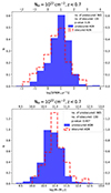 |
Fig. 4. Similar to Fig. 3 but using a limit of NH = 1022 cm−2 to classify AGN (taking into account the errors of the NH measurements). |
An alternative hypothesis proposed by Georgantopoulos et al. (2023) is that the variations in results across different studies could be attributed to the diverse luminosity ranges covered by the respective samples. For instance, AGN in the Boötes and XXM-XXL fields (Masoura et al. 2021; Mountrichas et al. 2021c) probe higher luminosities compared to those probed by sources in the COSMOS field (Lanzuisi et al. 2017; Georgantopoulos et al. 2023). This is also true when we compare the results between studies that used X-ray and optical criteria to classify the AGN. The latter have either used sources in the COSMOS field (e.g. Zou et al. 2019) that mainly probe low to intermediate LX AGN, or they have restricted their analysis to low luminosity systems at low redshift (e.g. Mountrichas et al. 2021c). To examine this hypothesis, we restricted our X-ray dataset to luminous sources by applying a luminosity cut at log [LX(erg s−1) > 44] (at z < 0.7), and we classified the AGN using an NH value of 1022 (using the lower and upper limits of NH) and repeated the analysis. There are 17 luminous and obscured AGN and 223 luminous and unobscured AGN. We detected a difference of 0.35 dex (based on the weighted median values) in the SFR of the two AGN populations. The obscured AGN appear to live in more massive systems compared to unobscured AGN (by 0.06 dex). However, none of these differences appeared to be statistically significant (p-value = 0.52 and 0.17 for the SFR and M*, respectively).
5.2. Eddington ratio of X-ray obscured and unobscured active galactic nuclei
The difference with the highest statistical significance that Georgantopoulos et al. (2023) reported was between the nEdd of obscured and unobscured sources (see e.g. their Table 3). Prompted by their results, we examined this difference in our dataset. For the dataset used in this part of our analysis, we did not have any available MBH, and therefore there were no nEdd measurements for our sources. Cross-matching our sample with the Wu & Shen (2022) catalogue (see Sect. 2) in which there are available nEdd measurements would constrain our dataset to only broad-line sources and exclude narrow-line AGN. In the next section, we examine whether nEdd depends on NH (for broad-line AGN). In order to include both broad- and narrow-line sources in our investigation, in place of nEdd, we examined the specific black hole accretion rate, λsBHAR, of obscured and unobscured AGN. We note that λsBHAR is the rate of the accretion onto the SMBH relative to the M* of the host galaxy. It is often used as a proxy of nEdd, particularly when MBH measurements are not available (e.g. Georgakakis et al. 2017; Aird et al. 2018; Mountrichas et al. 2021c; Pouliasis et al. 2022). For the calculation of λsBHAR, the following expression was used (e.g. Aird et al. 2018):
where kbol is a bolometric correction factor that converts the X-ray luminosity to AGN bolometric luminosity. We adopted the value of kbol = 25 (e.g. Georgakakis et al. 2017; Aird et al. 2018; Mountrichas et al. 2021c, 2022c).
Figure 5 presents the λsBHAR distributions of obscured and unobscured AGN using different NH thresholds to classify sources, as indicated at the top of each panel (taking into account the errors on the NH measurements). All distributions are weighted based on the LX and redshift of the sources. Table 2 presents the (weighted) median log λsBHAR of the obscured and unobscured AGN for NH = 1023 cm−2 and NH = 1022 cm−2. We found a difference of ∼0.1 − 0.2 dex in the λsBHAR values of the two populations. Specifically, we found obscured sources tend to have, on average, a lower λsBHAR compared to unobscured sources.. Based on the p-values derived using a KS test, this difference has a high statistical significance, regardless of the NH limit used. Similar p-values were found by applying MW and Kuiper tests.
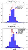 |
Fig. 5. Distributions of λsBHAR for obscured and unobscured AGN. The top panel presents the distributions using an NH threshold of 1023 cm−2 for the source classification. The bottom panel presents the results using NH = 1022 cm−2 to characterise sources. In both cases, the errors of the NH measurements have been taken into account (see text for more details). Distributions are also weighted based on the redshift and LX of the sources. |
Our results are in agreement with those reported in Georgantopoulos et al. (2023). We note that the difference we found appears smaller compared to the difference presented in the aforementioned study (∼0.3 dex). As we have already pointed out, we used stricter criteria in our analysis for the classification of AGN as obscured and unobscured compared to what was used in Georgantopoulos et al. (2023). Moreover, in Georgantopoulos et al. (2023), for the calculation of nEdd, they applied the same bolometric correction on LX to infer Lbol as in this study. However, they used MBH measurements derived by stellar velocity dispersions, σ; that is, they utilised a different scaling relation compared to our work.
We concluded that the obscured AGN tend to live in more massive systems compared to unobscured AGN at z < 0.7. The difference in M* is small (≈0.1 dex), but it appears to be statistically significant. Obscured sources also live in hosts that have a lower SFR, by ≈0.25 dex, than unobscured AGN; however, this difference is not statistically significant (< 2σ). Moreover, neither of these differences appears to be statistically significant for luminous AGN (log [LX(erg s−1) > 44] and/or when less strict criteria are used for the source classification (i.e. errors on NH are ignored). Based on our analysis, the difference between the two AGN populations with the highest statistical significance is that regarding the λsBHAR, which is a proxy of the nEdd.
5.3. Comparative analysis of super massive black hole characteristics, X-ray spectral attributes, and host galaxy properties
In the second part of our analysis, we examined the relationships among Lbol, MBH, and M* as a function of the X-ray obscuration (NH). We also investigated the correlation between the powerlaw slope, Γ, of the spectral model with the nEdd. For that purpose, we used the 271 X-ray AGN that are in common between the XMM catalogue and the Wu & Shen (2022) catalogue (see Sect. 4). Here and in the following (sub-) sections, we characterise as AGN with high NH those sources with log NH ≥ 1022 cm−2 using the mode value of NH that is available in our catalogue (i.e. without using the lower and upper limits of NH). There are 23 AGN with high NH values and 248 AGN with low NH values in our dataset. The reason for using this threshold is that it facilitates a better comparison with previous studies. Furthermore, we note that characterising an AGN with high NH based on requiring the lower limit of NH to be higher than 1023 cm−2 (1022 cm−2) would result in zero (seven) sources.
Figures 6–8 present the distributions of LX, M*, and MBH as a function of redshift, respectively, for the 271 X-ray AGN. All three properties increase with redshift regardless of the NH value of the source. A Spearman correlation analysis revealed that there is a significant correlation between LX, M*, and MBH with redshift, albeit these correlations appear higher in the case of sources with NH < 1022 cm−2 (Table 3). We note that in this part of our analysis, only broad-line (type 1) sources were included (see Sect. 2).
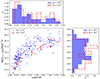 |
Fig. 6. X-ray luminosity, LX, as a function of redshift. AGN with log NH > 1022 cm−2 are marked with red circles, whereas sources with log NH < 1022 cm−2 are marked with blue triangles. |
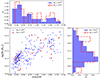 |
Fig. 7. Stellar mass, M*, as a function of redshift. AGN with log NH > 1022 cm−2 are marked with red circles, whereas sources with NH < 1022 cm−2 are marked with blue triangles. |
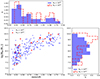 |
Fig. 8. Black hole mass, MBH, as a function of redshift. AGN with log NH > 1022 cm−2 are marked with red circles, whereas sources with NH < 1022 cm−2 are marked with blue triangles. |
p-values obtained from Spearman correlation analysis, assessing the correlations among LX, M*, MBH, and redshift.
5.3.1. Bolometric luminosity versus black hole mass
In Fig. 9, we plot the Lbol as a function of MBH. We chose to plot the Lbol measurements that are available in the Wu & Shen (2022) catalogue. We note that their Lbol calculations are in excellent agreement with the Lbol measurements from CIGALE. Specifically, the mean difference of the two calculations is 0.04 dex (with a dispersion of 0.36), and thus this choice does not affect our results and conclusions. The lines correspond to Lbol= LEdd (black long-dashed line), Lbol = 0.1 LEdd (green solid line), and Lbol = 0.01 LEdd (red dotted line). The vast majority of our AGN lie between Eddington ratios of 0.01 and 1, with a median value of nEdd = 0.14), in agreement with previous studies (e.g. Trump et al. 2009; Lusso et al. 2012; Sun et al. 2015; Suh et al. 2020; Mountrichas 2023). Different symbols correspond to different redshift intervals, as indicated in the legend of the plot. The median value of nEdd is 0.09 and 0.24 at z < 0.7 and 0.7 < z < 1.9, respectively.
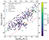 |
Fig. 9. Bolometric luminosity, Lbol, as a function of MBH. Different symbols correspond to different redshift intervals, as indicated in the legend. The lines correspond to Lbol = LEdd (black dashed line), Lbol = 0.1 LEdd (green solid line) and Lbol = 0.01 LEdd (red dotted line). Measurements are colour-coded based on the NH of each source. |
The measurements in Fig. 9 are colour-coded based on the NH of the sources. Although the AGN sample used in this part of our analysis consists of type 1 sources, there are a few AGN that present low levels of X-ray obscuration (NH ∼ 1022 cm−2). It is known that X-ray and optical obscuration do not necessarily coincide and several instances have been documented in the literature where type 1 AGN exhibit X-ray obscuration (e.g. Mateos et al. 2005, 2010; Scott et al. 2011; Shimizu et al. 2018; Kamraj et al. 2019; Masoura et al. 2020). Regarding the nEdd values of X-ray sources with high and low NH values, we did not find a difference among the two AGN populations. Specifically, the median values are nEdd = 0.12 and 0.15 for AGN with NH > 1022 cm−2 and AGN with NH < 1022 cm−2, respectively. A KS test yielded a p-value of 0.83 for the nEdd distributions of the two AGN classes.
5.3.2. Black hole mass versus stellar mass
Next in our analysis, we examined the correlation between MBH and M*. The results are presented in Fig. 10. A strong correlation was detected between the two parameters. Applying a Spearman correlation analysis yielded a p-value of 3.5 × 10⁻²⁹. A similar value was found using a Kendall correlation analysis (p-value = 8.1 × 10⁻²⁶). Strong correlations between MBH and M* were also found when we split the dataset into two redshift intervals. The p-values are shown in the legend of Fig. 10. In this case the correlations, although strong, were weaker compared to the correlation found for our full sample. This can be attributed to the narrower range of MBH and M* probed by the sources within distinct redshift intervals compared to the sources encompassing the entire redshift range (see Figs. 7 and 8). To validate this conjecture, we employed the AGN dataset spanning the complete redshift range (z ≤ 1.9); we restricted the (log of) M* and MBH ranges within 11.0 − 13.0 and 8.5 − 10, respectively (resembling the intervals embraced by AGN residing within 0.7 ≤ z ≤ 1.9); and we carried out a Spearman correlation analysis. This procedure resulted in a p-value of 0.008. Similarly, we obtained a p-value of 6 × 10⁻⁴ by limiting the M* and MBH ranges to 10.0 − 11.5 and 7.0 − 9.5 (akin to the intervals pertinent to AGN existing within z < 0.7).
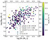 |
Fig. 10. Black hole mass, MBH, as a function of M*. Different symbols correspond to different redshift bins, as indicated in the legend. The p-values obtained by applying a Spearman correlation analysis for the full redshift range (z < 1.9) as well as at low redshift (z < 0.7) and high redshift (0.7 < z < 1.9) are also shown. Measurements are colour-coded based on the NH of each source. |
Prompted by the results of Sarria et al. (2010), who examined three X-ray AGN at z = 1 − 2, with NH = 1022.5 − 23.0 cm−2 and observed that they were consistent with the local MBH − M* relation, we colour coded the symbols in Fig. 10 based on the NH values of the sources. We noticed that sources with increased NH have a higher MBH for similar M* compared to sources with a lower NH. This is better illustrated in Fig. 11, where we mark AGN with NH values above and below 1022 cm−2 differently, as indicated in the legend of the plot. The different lines in Fig. 11 indicate the best fits for the various subsets acquired through the application of a least-squares analysis. As mentioned above, AGN with higher NH values tend to have more massive black holes compared to AGN with lower NH values at similar M*, at least up to log [M*(M⊙)] = 12.
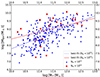 |
Fig. 11. Black hole mass, MBH, as a function of M* for sources with log NH > 1022 cm−2 (red circles) and sources with log NH < 1022 cm−2 (blue triangles). Different lines represent the best fits of the different subsets, as indicated in the legend. |
We also examined the ratio of MBH/M* as a function of redshift. Based on the results presented in the top panel of Fig. 12, the MBH/M* does not evolve with cosmic time up z < 2. The median log(MBH/M*) value was found at −2.63. This value is in agreement with most previous studies that measured the MBH/M* ratio in the local Universe (e.g. −2.85; Häring & Rix 2004) as well as at high redshifts (e.g. Suh et al. 2020; Mountrichas 2023). The bottom panel of Fig. 12 presents the distributions of the MBH/M* ratio at different redshift intervals. The median value of the MBH/M* ratio at z < 0.7 is −2.69, and at 0.7 < z < 1.9, it is −2.55. The application of KS tests confirmed that the distributions are similar (p-values > 0.9 among all redshift intervals).
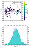 |
Fig. 12. Ratio of MBH to M*. The top panel presents the MBH − M* ratio as a function of redshift, and the bottom panel shows the distributions of the MBH − M* ratio at different redshift intervals. |
The results that appear in the top panel of Fig. 12 are colour-coded based on the NH of the sources. Sources with higher NH values seem to have a higher MBH/M* ratio. To examine this further, in Fig. 13, we plot the MBH/M* ratio as a function of NH. The blue line shows the best fit of the  relation for log NH < 22 cm−2, whereas the red line shows the best fit for log NH > 22 cm−2. The blue line is nearly flat, with a slope of 0.014 (standard error 0.079), which indicates that the MBH/M* ratio is almost constant for AGN with log NH < 22 cm−2. However, the best fit for AGN with log NH > 22 cm−2 has a slope of 0.69 (standard error 0.24), which indicates that the MBH/M* ratio increases with NH for X-ray AGN with high NH values. A Spearman correlation analysis revealed a p-value = 0.06 for the correlation between
  log NH for sources with log NH > 22 cm−2, which indicates a statistical significance of ∼2σ. The median value of the log MBH/M* ratio is -2.40 and -2.66 for AGN with NH > 1022 cm−2 and NH < 1022 cm−2, respectively. We note, though, that a larger number of sources with NH > 1022 cm−2 is required to formulate robust conclusions.
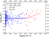 |
Fig. 13. Ratio of MBH to M* as a function of NH. |
In the preceding sections, we observed that obscured AGN live, on average, in galaxies with a higher M* compared to unobscured AGN. Moreover, obscured AGN tend to have a higher MBH compared to their unobscured counterparts at similar M*. When combined with the higher MBH/M* ratio within the AGN population displaying elevated NH values, assuming this holds true, it implies that the SMBH growth in the obscured phase is higher than the galaxy growth. This may suggest that the growth of the MBH occurs first, while the early stellar mass assembly may not be so efficient (Mountrichas et al. 2023).
5.3.3. Powerlaw slope versus Eddington ratio
We also investigated if there is a correlation between the powerlaw slope, Γ, of the X-ray spectral model and the nEdd. The results are shown in the top panel of Fig. 14. A strong correlation was found between Γ and nEdd (p-value = 8.1 × 10⁻⁷, applying both a Spearman and a Kendall correlation analysis). However, the correlation between the two parameters was also strong when we split the dataset into two redshift intervals; at 0.7 < z < 1.9, the p-value appears higher compared to the p-value obtained at z < 0.7 (see legend in the top panel of Fig. 14). This is most probably due to the different lines used for the calculation of the MBH and not a result of cosmic evolution. Risaliti et al. (2009) reported a strong correlation between the two parameters when the MBH was calculated using the H β line, while the authors reported a weaker correlation when the MBH was measured using the Mg II line. There are only 12 sources in our dataset with 0.7 < z < 1.9 that have MBH calculations from both lines; therefore, we could not test, in a robust manner, this hypothesis further. We also split the dataset into high and low LX, by applying a cut at log [LX(ergs−1)] = 44. A strong correlation was found both at high and low LX. The application of the Spearman correlation analysis gave p-values = 5.3 × 10⁻⁴ and 3.1 × 10⁻⁹ for log [LX(erg s−1)] > 44 and log [LX(ergs−1)] < 44, respectively.
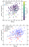 |
Fig. 14. Spectral photon index, Γ, as a function of nEdd. In the top panel, different symbols correspond to different redshift intervals, as indicated in the legend. The results are colour-coded based on the NH values of the sources. The p-values obtained by applying a Spearman correlation analysis are shown in the legend. The bottom panel shows the same relation but for X-ray AGN with NH > 1022 cm−2 (red circles) and AGN with NH < 1022 cm−2 (blue triangles). The p-values for the Γ − nEdd correlation for each AGN population are presented in the legend of the plot. The different lines correspond to the best fits using the total AGN sample (black dashed line), AGN with NH > 1022 cm−2 (red solid line), and AGN with NH < 1022 cm−2 (blue line). |
We further examined if this correlation between Γ and nEdd holds for different NH values. The results are shown in the bottom panel of Fig. 14. A strong correlation was found between Γ and nEdd for AGN with NH < 1022 cm−2. Application of the Spearman correlation analysis yielded p-value = 1.35 × 10⁻⁶ (p-value = 1.44 × 10⁻⁶, applying Kendall’s correlation analysis). No correlation was found, though, for the AGN population with NH > 1022 cm−2 (p-value = 0.47 and 0.53, from Spearman and Kendall correlation analysis, respectively). The different lines shown in the figure represent the best fits of the Γ − nEdd relation for the total AGN sample (black dashed line; Γ = 0.315× nEdd + 0.294), the AGN with NH < 1022 cm−2 (blue line; Γ = 0.306× nEdd + 2.303)), and for AGN with NH > 1022 cm−2 (red line; Γ = 0.083× nEdd + 1.565)). Similar results were obtained when we split the two AGN populations into two redshift intervals at z = 0.7. Furthermore, our observations hold when considering the associated uncertainties of Γ and nEdd. This was verified, by utilising the linmix module (Kelly 2007), which performs a linear regression between two parameters by repeatedly perturbing the datapoints within their uncertainties.
We find it worth pointing out that in Fig. 14 there are some sources with non-physical values (Γ > 2.5 or Γ < 1.5). Although their occurrence is relatively low among AGN with NH < 1022 cm−2 (15%), it becomes more pronounced (57%) for AGN with higher NH values. To examine whether this might influence the absence of a correlation between Γ and nEdd for AGN with NH > 1022 cm−2, we opted to exclude these sources and repeated the correlation analysis. However, even after this exclusion, we still did not observe a significant correlation between the two parameters for sources with elevated NH values. We find it essential to note, however, that this refinement in the analysis left us with a considerably reduced sample size, comprising only ten AGN with NH > 1022 cm−2.
The X-ray spectral index is sensitive to the properties of the accretion disc, such as temperature and ionisation state. Therefore, a correlation between the X-ray spectral index and nEdd for AGN with NH < 1022 cm−2 may imply that changes in the accretion rate can alter the structure and properties of the accretion disc, influencing the X-ray emission. The X-ray emission is also associated with a hot, optically thin corona of electrons above the accretion disc. The properties of the corona, such as its temperature and optical depth, can impact the X-ray spectral index. Thus, changes in the nEdd may lead to variations in the corona properties, affecting the X-ray spectrum. The AGN with NH < 1022 cm−2 allow for a clearer view of the inner regions of the accretion disc and the corona. Furthermore, in AGN with low NH, a more direct view of the accretion disc may allow for a better determination of the Eddington ratio.
Additionally, we investigated if this lack of correlation between the two parameters for the AGN population with NH > 1022 cm−2 is due to the small number of available sources. For that purpose, we randomly selected an equal number of AGN with NH < 1022 cm−2 to that with NH > 1022 cm−2, and we measured the correlation between Γ and nEdd. After 500 repetitions of this process, we obtained a median p-value of 0.047 from Spearman analysis (Kendall’s correlation analysis yielded p-value = 0.091). The p-value obtained for the simulated AGN with NH < 1022 cm−2 is about an order of magnitude lower compared to that obtained from the AGN with NH > 1022 cm−2. This indicates that the lack of correlation between Γ and nEdd for AGN with NH > 1022 cm−2 is intrinsic and not due to their smaller sample size. This result aligns with the Comptonisation models, wherein variations in the accretion rate have a more pronounced impact on the soft spectral component (which gets lost in absorbed sources) compared to the hard powerlaw photon index.
As already noted, λsBHAR is often used as a proxy of nEdd. Lopez et al. (2023) used X-ray selected AGN in the miniJPAS footprint and found, among other things, that the nEdd and λsBHAR have a difference of 0.6 dex. They attributed this difference to the scatter on the MBH − M* relation of their sources. A difference between nEdd and λsBHAR was also reported by Mountrichas & Buat (2023), albeit lower (∼0.25 dex), using AGN in the XMM-XXL field. Figure 15 presents a comparison between the two parameters for the 271 X-ray AGN that are in common between the XMM catalogue and the Wu & Shen (2022) catalogue. We found that, overall, there is good agreement between nEdd and λsBHAR, with a median difference of 0.10 dex. We stress that this comparison includes only broad-line AGN. We also confirm that this difference does not depend on NH, at least up to NH = 1022.5 − 23 cm−2, as probed by our dataset.
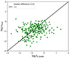 |
Fig. 15. Eddington ratio, Edd, vs. λsBHAR for the 271 AGN that are common between the XMM sample and the Wu & Shen (2022) catalogue. |
Since the nEdd measurements are in agreement with the λsBHAR calculations, we then examined the correlation between Γ and λsBHAR. We found similar results as those between Γ and nEdd. Specifically, a strong correlation was found between the two parameters for AGN with NH < 1022 cm−2 (p-value = 2.8 × 10⁻³), but no correlation was detected for sources with NH > 1022 cm−2 (p-value = 0.95). Prompted by these results, we utilised the larger AGN dataset used in Sect. 5.1 (i.e. before matching the XMM sources with the Wu & Shen 2022, catalogue) to examine the correlation between Γ and λsBHAR for the two AGN populations. This allowed us to investigate the Γ − λsBHAR relation using a significantly larger sample of obscured sources (130 AGN) that has been defined with stricter criteria (i.e. taking into account the uncertainties associated with NH) and, more importantly, to include narrow-line (type 2) AGN in our investigation. A Spearman correlation analysis yielded a p-value of 1.8 × 10⁻¹¹ for AGN with NH < 1022 cm−2 and 0.31 for AGN with NH > 1022 cm−2. We conclude that Γ and nEdd are correlated at all redshift and LX probed by our dataset. However, we did not detect such a correlation for AGN with increased NH values (NH > 1022 cm−2).
Previous studies have found contradictory results regarding whether there is a correlation between Γ and nEdd. Shemmer et al. (2008) used 35 unabsorbed type 1 radio quiet (RQ) AGN at z < 3.2 (25 out of the 35 sources were at z < 0.5) and found a significant correlation between Γ and nEdd. They concluded that a measurement of Γ and LX can provide an estimate of nEdd and MBH with a mean uncertainty of a factor less than or equal to three. Brightman et al. (2013) used 69 RQ AGN in the COSMOS and ECDFS fields at z < 2 and found a significant correlation between the X-ray spectral index and nEdd. However, based on their analysis, the scatter of the Γ − nEdd relation is large, and thus the relation is only suitable for large samples and not for individual sources. We note, though, that the Lbol of their sources was calculated following a mix of different methods (SED fitting and bolometric correction to the LX), and this may contribute to the scatter. Trakhtenbrot et al. (2017) used 228 hard X-ray-selected AGN from the Swift/Bat AGN Spectroscopic Survey (BASS) and found a very weak but statistically significant correlation between Γ and nEdd. Nonetheless, their MBH measurements come from several different methods (see their Sect. 2.3), and they reported that the correlation was weaker or even absent within their different subsets. More recently, Kamraj et al. (2022) used 195 Seyfert 1 AGN in the local Universe (z < 0.2) with NuSTAR and Swift/XRT or XMM observations. They studied the correlation between the X-ray spectral index and nEdd using three models to fit the X-ray spectra of their sources. They found considerable scatter and no strong trend between Γ and nEdd for all the spectral models they applied. They concluded that the Γ − nEdd may not be universal nor robust and could vary with the choice of the sample, the luminosity range probed, and the energy range of X-ray data used in the analysis. We note that their MBH estimates come from the second data release of the optical measurements from the BASS survey and were inferred using a compilation of different techniques (e.g. broad-line measurements from optical spectra, stellar velocity dispersions, reverberation mapping), which could increase the scatter in the Γ − nEdd and weaken any possible correlation.
Combining the results of our analysis with those from previous works, we conclude that caution has to be taken when compiling results from different studies that have used different methods to measure the MBH and the Lbol. Furthermore, the correlation between Γ and nEdd may not be universal and could (also) depend on the level of the X-ray obscuration of the sources.
6. Conclusions
The parent sample of this work includes ∼35 000 X-ray AGN included in the 4XMM-DR11 catalogue for which there are available X-ray spectra fitting measurements. To measure the host galaxy properties of these sources, we matched them with multiwavelength datasets and constructed their SEDs. Using the CIGALE SED fitting algorithm, we calculated the SFR and M* of the AGN. Our analysis demanded stringent selection criteria to ensure that only AGN with dependable X-ray spectral and SED fitting measurements were incorporated in our investigation. There were 1443 AGN that fulfilled these requirements. We then applied strict criteria using the NH values and their associated uncertainties to classify sources into obscured and unobscured AGN and compared their SMBH and host galaxy properties. Our main findings are the following:
-
Obscured AGN tend to live in more massive systems (by ∼0.1 dex) compared to unobscured AGN. The difference, although small, appears to be statistically significant. Obscured sources also tend to live in galaxies with a lower SFR (by ∼0.25 dex) compared to their unobscured counterparts; however, this difference is not statistically significant. The results do not depend on the NH threshold used to classify AGN (NH = 1023 cm−2 or NH = 1022 cm−2), and the differences are not statistically significant at high LX (log [LX(erg s−1)] > 44) nor if we disregard the errors associated with the NH measurements.
-
Unobscured AGN have, on average, higher specific black hole accretion rates (a proxy of the Eddington ratio) compared to unobscured sources. The difference is 0.1 − 0.2 dex and appears to have a high statistical significance.
Furthermore, we cross-matched our dataset with the catalogue of Wu & Shen (2022), which includes measurements for the MBH, Lbol, and Eddington ratio, among others, for ∼750 000 QSOs from SDSS. There are 271 type 1 AGN in common between the two datasets up to a redshift of 1.9. We studied the nEdd and MBH/M* ratio of the two AGN populations, and we examined if there is a correlation between Γ and nEdd. Our main results are summarised as follows:
-
Type 1 AGN with NH > 1022 cm−2 tend to have a higher MBH compared to type 1 sources with lower NH values at similar M*.
-
For type 1 AGN, the MBH/M* ratio is nearly constant, with NH up to NH = 1022 cm−2. However, our results suggest that the MBH/M* ratio increases at higher NH values.
-
A correlation was found between the spectral photon index, Γ, and the Eddington ratio, nEdd, for type 1 AGN with NH < 1022 cm−2.
The findings of our work indicate that the inconsistent results among previous studies regarding the host galaxy properties of obscured and unobscured AGN could mainly be due to the different luminosities probed. Additionally, our analysis indicates that during the obscured phase, SMBH growth exceeds that of the host galaxies, potentially implying a sequential growth pattern where MBH develops first, while early stellar mass assembly might not be as efficient. Furthermore, the disparities in previous research regarding the correlation between Γ and nEdd may also be partly attributed to differences in the fraction of obscured and unobscured AGN within the samples used in those studies.
Acknowledgments
This project has received funding from the European Union’s Horizon 2020 research and innovation program under grant agreement no. 101004168, the XMM2ATHENA project. This research has made use of data obtained from the 4XMM XMM-Newton serendipitous source catalogue compiled by the 10 institutes of the XMM-Newton Survey Science Centre selected by ESA. Funding for the Sloan Digital Sky Survey V has been provided by the Alfred P. Sloan Foundation, the Heising-Simons Foundation, the National Science Foundation, and the Participating Institutions. SDSS acknowledges support and resources from the Center for High-Performance Computing at the University of Utah. The SDSS web site is www.sdss.org. SDSS is managed by the Astrophysical Research Consortium for the Participating Institutions of the SDSS Collaboration, including the Carnegie Institution for Science, Chilean National Time Allocation Committee (CNTAC) ratified researchers, the Gotham Participation Group, Harvard University, Heidelberg University, The Johns Hopkins University, L’École polytechnique fédérale de Lausanne (EPFL), Leibniz-Institut fur Astrophysik Potsdam (AIP), Max-Planck-Institut fur Astronomie (MPIA Heidelberg), Max-Planck-Institut fur Extraterrestrische Physik (MPE), Nanjing University, National Astronomical Observatories of China (NAOC), New Mexico State University, The Ohio State University, Pennsylvania State University, Smithsonian Astrophysical Observatory, Space Telescope Science Institute (STScI), the Stellar Astrophysics Participation Group, Universidad Nacional Autónoma de México, University of Arizona, University of Colorado Boulder, University of Illinois at Urbana-Champaign, University of Toronto, University of Utah, University of Virginia, Yale University, and Yunnan University. The Pan-STARRS1 Surveys (PS1) and the PS1 public science archive have been made possible through contributions by the Institute for Astronomy, the University of Hawaii, the Pan-STARRS Project Office, the Max-Planck Society and its participating institutes, the Max Planck Institute for Astronomy, Heidelberg and the Max Planck Institute for Extraterrestrial Physics, Garching, The Johns Hopkins University, Durham University, the University of Edinburgh, the Queen’s University Belfast, the Harvard-Smithsonian Center for Astrophysics, the Las Cumbres Observatory Global Telescope Network Incorporated, the National Central University of Taiwan, the Space Telescope Science Institute, the National Aeronautics and Space Administration under Grant No. NNX08AR22G issued through the Planetary Science Division of the NASA Science Mission Directorate, the National Science Foundation Grant No. AST-1238877, the University of Maryland, Eotvos Lorand University (ELTE), the Los Alamos National Laboratory, and the Gordon and Betty Moore Foundation. This publication makes use of data products from the Wide-field Infrared Survey Explorer, which is a joint project of the University of California, Los Angeles, and the Jet Propulsion Laboratory/California Institute of Technology, funded by the National Aeronautics and Space Administration. This research has made use of TOPCAT version 4.8 (Taylor 2005) and Astropy (Astropy Collaboration 2022).
References
- Aird, J., Coil, A. L., & Georgakakis, A. 2018, MNRAS, 474, 1225 [NASA ADS] [CrossRef] [Google Scholar]
- Arnaud, K. A. 1996, ASP Conf. Ser., 101, 17 [Google Scholar]
- Astropy Collaboration (Price-Whelan, A. M., et al.) 2022, ApJ, 935, 167 [NASA ADS] [CrossRef] [Google Scholar]
- Bolton, A. S., Schlegel, D. J., Aubourg, É., et al. 2012, AJ, 144, 144 [NASA ADS] [CrossRef] [Google Scholar]
- Boquien, M., Burgarella, D., Roehlly, Y., et al. 2019, A&A, 622, A103 [NASA ADS] [CrossRef] [EDP Sciences] [Google Scholar]
- Boyle, B. J., Shanks, T., Croom, S. M., et al. 2000, MNRAS, 317, 1014 [NASA ADS] [CrossRef] [Google Scholar]
- Brightman, M., Silverman, J. D., Mainieri, V., et al. 2013, MNRAS, 433, 2485 [Google Scholar]
- Bruzual, G., & Charlot, S. 2003, MNRAS, 344, 1000 [NASA ADS] [CrossRef] [Google Scholar]
- Buat, V., Ciesla, L., Boquien, M., Małek, K., & Burgarella, D. 2019, A&A, 632, A79 [NASA ADS] [CrossRef] [EDP Sciences] [Google Scholar]
- Buat, V., Mountrichas, G., Yang, G., et al. 2021, A&A, 654, A93 [NASA ADS] [CrossRef] [EDP Sciences] [Google Scholar]
- Buchner, J. 2019, PASP, 131, 108005 [Google Scholar]
- Buchner, J., Georgakakis, A., Nandra, K., et al. 2014, A&A, 564, A125 [NASA ADS] [CrossRef] [EDP Sciences] [Google Scholar]
- Buchner, J., Brightman, M., Balokovic, M., et al. 2021, A&A, 651, A58 [NASA ADS] [CrossRef] [EDP Sciences] [Google Scholar]
- Chabrier, G. 2003, PASP, 115, 763 [Google Scholar]
- Charlot, S., & Fall, S. M. 2000, ApJ, 539, 718 [Google Scholar]
- Ciotti, L., & Ostriker, J. P. 1997, ApJ, 487, L105 [NASA ADS] [CrossRef] [Google Scholar]
- Dale, D. A., Helou, G., Magdis, G. E., et al. 2014, ApJ, 784, 83 [Google Scholar]
- Davis, S. W., & Laor, A. 2011, ApJ, 728, 98 [NASA ADS] [CrossRef] [Google Scholar]
- Esparza-Arredondo, D., Gonzalez-Martín, O., Dultzin, D., et al. 2021, A&A, 651, A91 [NASA ADS] [CrossRef] [EDP Sciences] [Google Scholar]
- Evans, P. A., Page, K. L., Osborne, J. P., et al. 2020, ApJS, 247, 54 [Google Scholar]
- Ferrarese, L., & Merritt, D. 2000, ApJ, 539, 9 [Google Scholar]
- Georgakakis, A., Aird, J., Schulze, A., et al. 2017, MNRAS, 471, 1976 [NASA ADS] [CrossRef] [Google Scholar]
- Georgantopoulos, I., Pouliasis, E., Mountrichas, G., et al. 2023, A&A, 673, A67 [NASA ADS] [CrossRef] [EDP Sciences] [Google Scholar]
- Häring, N., & Rix, H.-W. 2004, ApJ, 604, L89 [Google Scholar]
- Hopkins, P. F., Hernquist, L., Cox, T. J., et al. 2006, ApJS, 163, 1 [Google Scholar]
- Kamraj, N., Balokovic, M., Brightman, M., et al. 2019, ApJ, 887, 255 [NASA ADS] [CrossRef] [Google Scholar]
- Kamraj, N., Brightman, M., Harrison, F. A., et al. 2022, ApJ, 927, 42 [NASA ADS] [CrossRef] [Google Scholar]
- Kelly, B. C. 2007, ApJ, 665, 1489 [Google Scholar]
- Koutoulidis, L., Mountrichas, G., Georgantopoulos, I., Pouliasis, E., & Plionis, M. 2022, A&A, 658, A35 [NASA ADS] [CrossRef] [EDP Sciences] [Google Scholar]
- Lanzuisi, G., Delvecchio, I., Berta, S., et al. 2017, A&A, 602, A123 [NASA ADS] [CrossRef] [EDP Sciences] [Google Scholar]
- Lopez, I. E., Brusa, M., Bonoli, S., et al. 2023, A&A, 672, A137 [NASA ADS] [CrossRef] [EDP Sciences] [Google Scholar]
- Lusso, E., Comastri, A., Simmons, B. D., et al. 2012, MNRAS, 425, 623 [Google Scholar]
- Lyke, B. W., Higley, A. N., McLane, J. N., et al. 2020, ApJS, 250, 8 [NASA ADS] [CrossRef] [Google Scholar]
- Magorrian, J., Tremaine, S., Richstone, D., et al. 1998, AJ, 115, 2285 [Google Scholar]
- Małek, K., Buat, V., Roehlly, Y., et al. 2018, A&A, 620, A50 [Google Scholar]
- Marinucci, A., Bianchi, S., Matt, G., et al. 2016, MNRAS, 456, L94 [Google Scholar]
- Masoura, V. A., Mountrichas, G., Georgantopoulos, I., et al. 2018, A&A, 618, A31 [NASA ADS] [CrossRef] [EDP Sciences] [Google Scholar]
- Masoura, V. A., Georgantopoulos, I., Mountrichas, G., et al. 2020, A&A, 638, A45 [NASA ADS] [CrossRef] [EDP Sciences] [Google Scholar]
- Masoura, V. A., Mountrichas, G., Georgantopoulos, I., & Plionis, M. 2021, A&A, 646, A167 [EDP Sciences] [Google Scholar]
- Mateos, S., Barcons, X., Carrera, F. J., et al. 2005, A&A, 444, 79 [NASA ADS] [CrossRef] [EDP Sciences] [Google Scholar]
- Mateos, S., Carrera, F. J., Page, M. J., et al. 2010, A&A, 510, A35 [NASA ADS] [CrossRef] [EDP Sciences] [Google Scholar]
- Merloni, A., Bongiorno, A., Brusa, M., et al. 2014, MNRAS, 437, 3550 [Google Scholar]
- Mountrichas, G. 2023, A&A, 672, A98 [NASA ADS] [CrossRef] [EDP Sciences] [Google Scholar]
- Mountrichas, G., & Buat, V. 2023, A&A, 679, A151 [NASA ADS] [CrossRef] [EDP Sciences] [Google Scholar]
- Mountrichas, G., & Shankar, F. 2023, MNRAS, 518, 2088 [Google Scholar]
- Mountrichas, G., Georgakakis, A., & Georgantopoulos, I. 2019, MNRAS, 483, 1374 [NASA ADS] [CrossRef] [Google Scholar]
- Mountrichas, G., Buat, V., Georgantopoulos, I., et al. 2021a, A&A, 653, A70 [NASA ADS] [CrossRef] [EDP Sciences] [Google Scholar]
- Mountrichas, G., Buat, V., Yang, G., et al. 2021b, A&A, 646, A29 [EDP Sciences] [Google Scholar]
- Mountrichas, G., Buat, V., Yang, G., et al. 2021c, A&A, 653, A74 [NASA ADS] [CrossRef] [EDP Sciences] [Google Scholar]
- Mountrichas, G., Buat, V., Yang, G., et al. 2022a, A&A, 663, A130 [NASA ADS] [CrossRef] [EDP Sciences] [Google Scholar]
- Mountrichas, G., Buat, V., Yang, G., et al. 2022b, A&A, 667, A145 [NASA ADS] [CrossRef] [EDP Sciences] [Google Scholar]
- Mountrichas, G., Masoura, V. A., Xilouris, E. M., et al. 2022c, A&A, 661, A108 [NASA ADS] [CrossRef] [EDP Sciences] [Google Scholar]
- Mountrichas, G., Yang, G., Buat, V., et al. 2023, A&A, 675, A137 [NASA ADS] [CrossRef] [EDP Sciences] [Google Scholar]
- Nenkova, M., Ivezić, Ž., & Elitzur, M. 2002, ApJ, 570, L9 [NASA ADS] [CrossRef] [Google Scholar]
- Netzer, H. 2015, ARA&A, 53, 365 [Google Scholar]
- Ogawa, S., Ueda, Y., Tanimoto, A., & Yamada, S. 2021, ApJ, 906, 84 [NASA ADS] [CrossRef] [Google Scholar]
- Pouliasis, E., Mountrichas, G., Georgantopoulos, I., et al. 2022, A&A, 667, A56 [NASA ADS] [CrossRef] [EDP Sciences] [Google Scholar]
- Ricci, C., Ho, L. C., Fabian, A. C., et al. 2018, MNRAS, 480, 1819 [NASA ADS] [CrossRef] [Google Scholar]
- Risaliti, G., Young, M., & Elvis, M. 2009, ApJ, 700, L6 [NASA ADS] [CrossRef] [Google Scholar]
- Ruiz, A., Corral, A., Mountrichas, G., & Georgantopoulos, I. 2018, A&A, 618, A52 [NASA ADS] [CrossRef] [EDP Sciences] [Google Scholar]
- Sarria, J. E., Maiolino, R., Franca, F. L., et al. 2010, A&A, 522, L3 [NASA ADS] [CrossRef] [EDP Sciences] [Google Scholar]
- Scott, A. E., Stewart, G. C., Mateos, S., et al. 2011, MNRAS, 417, 992 [NASA ADS] [CrossRef] [Google Scholar]
- Shemmer, O., Brandt, W. N., Netzer, H., Maiolino, R., & Kaspi, S. 2008, ApJ, 682, 81 [Google Scholar]
- Shimizu, T. T., Davies, R. I., Koss, M., et al. 2018, ApJ, 856, 154 [NASA ADS] [CrossRef] [Google Scholar]
- Sobolewska, M. A., & Papadakis, I. E. 2009, MNRAS, 399, 1597 [NASA ADS] [CrossRef] [Google Scholar]
- Sobral, D., Smail, I., Best, P. N., et al. 2013, MNRAS, 428, 1128 [NASA ADS] [CrossRef] [Google Scholar]
- Somerville, R. S., Hopkins, P. F., Cox, T. J., Robertson, B. E., & Hernquist, L. 2008, MNRAS, 391, 481 [NASA ADS] [CrossRef] [Google Scholar]
- Stalevski, M., Fritz, J., Baes, M., Nakos, T., & Popović, L. Č. 2012, MNRAS, 420, 2756 [Google Scholar]
- Stalevski, M., Ricci, C., Ueda, Y., et al. 2016, MNRAS, 458, 2288 [Google Scholar]
- Suh, H., Civano, F., Trakhtenbrot, B., et al. 2020, ApJ, 889, 32 [NASA ADS] [CrossRef] [Google Scholar]
- Sun, M., Trump, J. R., Brandt, W. N., et al. 2015, ApJ, 802, 14 [NASA ADS] [CrossRef] [Google Scholar]
- Taylor, M. B. 2005, in Astronomical Data Analysis Software and Systems XIV, eds. P. Shopbell, M. Britton, & R. Ebert, ASP Conf. Ser., 347, 29 [Google Scholar]
- Trakhtenbrot, B., Ricci, C., Koss, M. J., et al. 2017, MNRAS, 470, 800 [NASA ADS] [CrossRef] [Google Scholar]
- Tranin, H., Godet, O., Webb, N., & Primorac, D. 2022, A&A, 657, A138 [NASA ADS] [CrossRef] [EDP Sciences] [Google Scholar]
- Tristram, K. R. W., Meisenheimer, K., Jaffe, W., et al. 2007, A&A, 474, 837 [NASA ADS] [CrossRef] [EDP Sciences] [Google Scholar]
- Trump, J. R., Impey, C. D., Elvis, M., et al. 2009, ApJ, 696, 1195 [NASA ADS] [CrossRef] [Google Scholar]
- Urry, C. M., & Padovani, P. 1995, PASP, 107, 803 [NASA ADS] [CrossRef] [Google Scholar]
- Vasudevan, R. V., & Fabian, A. C. 2007, MNRAS, 381, 1235 [NASA ADS] [CrossRef] [Google Scholar]
- Villa-Velez, J. A., Buat, V., Theule, P., Boquien, M., & Burgarella, D. 2021, A&A, 654, A153 [NASA ADS] [CrossRef] [EDP Sciences] [Google Scholar]
- Webb, N. A., Coriat, M., Traulsen, I., et al. 2020, A&A, 641, A136 [NASA ADS] [CrossRef] [EDP Sciences] [Google Scholar]
- Webb, N. A., Carrera, F. J., Schwope, A., et al. 2023, Astron. Nachr., 344, e20220102 [Google Scholar]
- Wu, Q., & Shen, Y. 2022, ApJS, 263, 42 [NASA ADS] [CrossRef] [Google Scholar]
- Yang, G., Boquien, M., Buat, V., et al. 2020, MNRAS, 491, 740 [Google Scholar]
- Yang, G., Boquien, M., Brandt, W. N., et al. 2022, ApJ, 927, 192 [NASA ADS] [CrossRef] [Google Scholar]
- Zou, F., Yang, G., Brandt, W. N., & Xue, Y. 2019, ApJ, 878, 11 [Google Scholar]
All Tables
Models and the values for their free parameters used by CIGALE for the SED fitting.
p-values obtained from Spearman correlation analysis, assessing the correlations among LX, M*, MBH, and redshift.
All Figures
|
Fig. 1. Example of a source spectrum and model fit (left panels), including the background modelling (right panels) for the PN (top panels) and MOS (bottom panels). |
| In the text | |
|
Fig. 2. Distribution of the 1443 X-ray AGN in the LX-redshift plane. |
| In the text | |
|
Fig. 3. Host galaxy properties of X-ray obscured (red dashed line histograms) and unobscured AGN (blue shaded histograms). Sources are classified as obscured when the lower limit of their NH value is higher than 1023 cm−2. We classified AGN as unobscured if the upper limit of their NH value is below 1023 cm−2. The top panel presents the SFR distributions of the two AGN populations. The bottom panel shows their M* distributions. The number of sources and the p-values obtained by applying a KS test are shown in the legend of the plots. Distributions are weighted based on the redshift and LX of the sources. |
| In the text | |
|
Fig. 4. Similar to Fig. 3 but using a limit of NH = 1022 cm−2 to classify AGN (taking into account the errors of the NH measurements). |
| In the text | |
|
Fig. 5. Distributions of λsBHAR for obscured and unobscured AGN. The top panel presents the distributions using an NH threshold of 1023 cm−2 for the source classification. The bottom panel presents the results using NH = 1022 cm−2 to characterise sources. In both cases, the errors of the NH measurements have been taken into account (see text for more details). Distributions are also weighted based on the redshift and LX of the sources. |
| In the text | |
|
Fig. 6. X-ray luminosity, LX, as a function of redshift. AGN with log NH > 1022 cm−2 are marked with red circles, whereas sources with log NH < 1022 cm−2 are marked with blue triangles. |
| In the text | |
|
Fig. 7. Stellar mass, M*, as a function of redshift. AGN with log NH > 1022 cm−2 are marked with red circles, whereas sources with NH < 1022 cm−2 are marked with blue triangles. |
| In the text | |
|
Fig. 8. Black hole mass, MBH, as a function of redshift. AGN with log NH > 1022 cm−2 are marked with red circles, whereas sources with NH < 1022 cm−2 are marked with blue triangles. |
| In the text | |
|
Fig. 9. Bolometric luminosity, Lbol, as a function of MBH. Different symbols correspond to different redshift intervals, as indicated in the legend. The lines correspond to Lbol = LEdd (black dashed line), Lbol = 0.1 LEdd (green solid line) and Lbol = 0.01 LEdd (red dotted line). Measurements are colour-coded based on the NH of each source. |
| In the text | |
|
Fig. 10. Black hole mass, MBH, as a function of M*. Different symbols correspond to different redshift bins, as indicated in the legend. The p-values obtained by applying a Spearman correlation analysis for the full redshift range (z < 1.9) as well as at low redshift (z < 0.7) and high redshift (0.7 < z < 1.9) are also shown. Measurements are colour-coded based on the NH of each source. |
| In the text | |
|
Fig. 11. Black hole mass, MBH, as a function of M* for sources with log NH > 1022 cm−2 (red circles) and sources with log NH < 1022 cm−2 (blue triangles). Different lines represent the best fits of the different subsets, as indicated in the legend. |
| In the text | |
|
Fig. 12. Ratio of MBH to M*. The top panel presents the MBH − M* ratio as a function of redshift, and the bottom panel shows the distributions of the MBH − M* ratio at different redshift intervals. |
| In the text | |
|
Fig. 13. Ratio of MBH to M* as a function of NH. |
| In the text | |
|
Fig. 14. Spectral photon index, Γ, as a function of nEdd. In the top panel, different symbols correspond to different redshift intervals, as indicated in the legend. The results are colour-coded based on the NH values of the sources. The p-values obtained by applying a Spearman correlation analysis are shown in the legend. The bottom panel shows the same relation but for X-ray AGN with NH > 1022 cm−2 (red circles) and AGN with NH < 1022 cm−2 (blue triangles). The p-values for the Γ − nEdd correlation for each AGN population are presented in the legend of the plot. The different lines correspond to the best fits using the total AGN sample (black dashed line), AGN with NH > 1022 cm−2 (red solid line), and AGN with NH < 1022 cm−2 (blue line). |
| In the text | |
|
Fig. 15. Eddington ratio, Edd, vs. λsBHAR for the 271 AGN that are common between the XMM sample and the Wu & Shen (2022) catalogue. |
| In the text | |
Current usage metrics show cumulative count of Article Views (full-text article views including HTML views, PDF and ePub downloads, according to the available data) and Abstracts Views on Vision4Press platform.
Data correspond to usage on the plateform after 2015. The current usage metrics is available 48-96 hours after online publication and is updated daily on week days.
Initial download of the metrics may take a while.