| Issue |
A&A
Volume 684, April 2024
|
|
|---|---|---|
| Article Number | A204 | |
| Number of page(s) | 15 | |
| Section | Extragalactic astronomy | |
| DOI | https://doi.org/10.1051/0004-6361/202348161 | |
| Published online | 25 April 2024 | |
Evidence of evolution of the black hole mass function with redshift⋆
1
Dipartimento di Fisica “E. Fermi”, Università di Pisa, Largo Bruno Pontecorvo 3, 56127 Pisa, Italy
e-mail: stefano.rinaldi@uni-heidelberg.de, walter.delpozzo@unipi.it
2
INFN, Sezione di Pisa, Largo Bruno Pontecorvo 3, 56127 Pisa, Italy
3
Institut für Theoretische Astrophysik, ZAH, Universität Heidelberg, Albert-Ueberle-Str. 2, 69120 Heidelberg, Germany
e-mail: mapelli@uni-heidelberg.de
4
IGFAE, University of Santiago de Compostela, Rúa de Xoaquín Díaz de Rábago, 15782 Santiago de Compostela, Spain
Received:
4
October
2023
Accepted:
10
February
2024
Aims. We investigate the observed distribution of the joint primary mass, mass ratio, and redshift of astrophysical black holes using the gravitational wave events detected by the LIGO-Virgo-KAGRA collaboration and included in the third gravitational wave transient catalogue.
Methods. We reconstructed this distribution using Bayesian non-parametric methods, which are data-driven models able to infer arbitrary probability densities under minimal mathematical assumptions.
Results. We find evidence that both the primary mass and mass-ratio distribution evolve with redshift: our analysis shows the presence of two distinct subpopulations in the primary mass−redshift plane, with the lighter population, ≲20 M⊙, disappearing at higher redshifts, z > 0.4. The mass-ratio distribution shows no support for symmetric binaries.
Conclusions. The observed population of coalescing binary black holes evolves with look-back time, suggesting a trend in metallicity with redshift and/or the presence of multiple redshift-dependent formation channels.
Key words: gravitation / gravitational waves / stars: black holes
Movies associated to Figs. 3 and 4 are available at https://www.aanda.org.
© The Authors 2024
 Open Access article, published by EDP Sciences, under the terms of the Creative Commons Attribution License (https://creativecommons.org/licenses/by/4.0), which permits unrestricted use, distribution, and reproduction in any medium, provided the original work is properly cited.
This article is published in open access under the Subscribe to Open model. Subscribe to A&A to support open access publication.
1. Introduction
GW150914 (Abbott et al. 2016a), the first gravitational wave (GW) event detected by the two LIGO detectors (Aasi et al. 2015) during the first observing run (O1), was the first direct measurement of the intrinsic properties of a binary black hole (BBH). The two compact objects that compose this system were a surprise to the astrophysical community: before GW150914, stellar-sized black holes (BHs) were studied mainly via single-line spectroscopic binaries from the very first observation of the BH in the X-ray source Cygnus X-1 (Byram et al. 1966; Bahcall et al. 1978). The mass distribution for such objects was modelled as a Gaussian distribution centred at 7.8 M⊙ with a standard deviation of 1.2 M⊙ (Özel et al. 2010). In contrast, the primary and secondary masses of GW150914, of namely  and
and  respectively (Abbott et al. 2016b, 2024), are significantly higher than the maximum BH mass observed in Milky Way X-ray binaries (Farr et al. 2011). A common interpretation, although still controversial in its details, is that the mass of a BH depends on the metallicity of its stellar progenitor, with metal-poor stars losing less mass by stellar winds and leading to the formation of more massive compact remnants than metal-rich stars (e.g. Heger et al. 2003; Mapelli et al. 2009, 2010; Zampieri & Roberts 2009; Belczynski et al. 2010).
Joined by the Virgo detector (Acernese et al. 2015) during the second observing run (O2) in 2017, by KAGRA (Aso et al. 2013; Akutsu 2020) in 2020 at the end of the third run (O3), and expected to include LIGO-India (Iyer et al. 2011) during the next decade, the LIGO-Virgo-KAGRA (LVK) collaboration has detected almost 100 GW signals to date, most of them generated by BBH coalescence (Abbott et al. 2023b). As the LVK collaboration is now in the middle of the fourth observing run (O4), this number is expected to grow in the upcoming months.
These observations confirm that the mass distribution inferred from Galactic BHs does not describe the general BBHs across the Universe, therefore suggesting that either coalescing BBHs follow different evolutionary paths from Galactic BHs, or that they have a different origin altogether. To discriminate among the various proposed scenarios, or unveil new ones, several groups have put considerable effort into studying BBH populations (Abbott et al. 2019, 2021b, 2023c; Talbot & Thrane 2018; Stevenson et al. 2019; Edelman et al. 2021; Fishbach et al. 2021; Roulet et al. 2021; Galaudage et al. 2021; Bouffanais et al. 2021; Stevenson & Clarke 2022; Callister & Farr 2024; Sadiq et al. 2024).
Current theoretical models propose several different formation channels for astrophysical BBHs. Among those, the most highly considered in the literature are isolated evolution (e.g. Bethe & Brown 1998; Belczynski et al. 2002; Dominik et al. 2012; Eldridge & Stanway 2016; Stevenson et al. 2017; Klencki et al. 2018; Kruckow et al. 2018; Iorio et al. 2023; Fragos et al. 2023; Briel et al. 2023; Srinivasan et al. 2023) and dynamical assembly in star clusters (e.g. Portegies Zwart & McMillan 2000; Banerjee et al. 2010; Rodriguez et al. 2016a; Mapelli 2016; Askar et al. 2017; Samsing 2018; Banerjee 2018; Di Carlo et al. 2020; Kumamoto et al. 2020; Kremer et al. 2020; Fragione & Silk 2020; Arca Sedda et al. 2021; Dall’Amico et al. 2021; Romero-Shaw et al. 2022) or active galactic nucleus (AGN) discs (e.g. McKernan et al. 2012, 2018; Bartos et al. 2017; Tagawa et al. 2020, 2021; Li et al. 2021b; Samsing et al. 2022; Vaccaro et al. 2024). Given the large observed masses in BBHs, it has also been proposed that at least one of the two BHs composing the detected binary may have already undergone a merger (Miller & Hamilton 2002; Gerosa & Berti 2017; Fishbach et al. 2017, 2022; Rodriguez et al. 2019; Antonini et al. 2019; Kimball et al. 2021; Mapelli et al. 2021; Gerosa & Fishbach 2021; Mould et al. 2022; Fragione & Rasio 2023; Rodriguez 2023).
The processes that stars go through during their lifetime are expected to leave signatures in the BH astrophysical distributions. For example, stellar winds (Vink et al. 2001; Lamers & Levesque 2017), core-collapse supernovae (Fryer et al. 2012; Schneider et al. 2021), envelope removal after common envelope (Hurley et al. 2002), and pulsational pair-instability supernovae (Heger et al. 2003; Woosley et al. 2015) result in non-negligible mass loss for the star. In addition to this, there is also the possibility that the BH is not of astrophysical origin, as in the case of primordial BHs (Carr 1975).
The LVK collaboration explored the properties of BBH populations and of individual BHs in a series of papers (Abbott et al. 2019, 2021b, 2023c) using different parametric and semi-parametric phenomenological models. In particular, the BH mass distribution is modelled after the initial stellar mass function (Salpeter 1955; Kroupa 2001) and revolves around a power-law model. Several additional features have been included throughout the years, such as a hard high-mass cutoff and a power-law distribution for the mass ratio (Fishbach & Holz 2017; Wysocki et al. 2019), or a Gaussian feature at around 35 − 40 M⊙ (Talbot & Thrane 2018), resulting in the so-called ‘POWERLAW+PEAK’ model. This model, described in Appendix B.1b of Abbott et al. (2023c), is the fiducial population model for LVK analysis.
Such models follow a phenomenological approach: they are based on the underlying physics, but capturing the many facets of astrophysical processes is beyond their scope. Moreover, these models are constrained to a given functional form that may or may not represent the underlying population. As a consequence, inferences based on these models could be biased if some of the features of the BH distribution are not properly accounted for.
Nonetheless, building a reliable parametric model that takes into account the complexity of astrophysical models is a formidable task: to date, and to the best of our knowledge, no all-encompassing parametric model has been proposed, although mixture models have begun to be explored. For instance, Zevin et al. (2021) show that single-channel models are disfavoured compared to models that include multiple channels.
An alternative route for the inference of BBH astrophysics – based on an opposing approach to the all-encompassing model – is to use the so-called non-parametric methods. These methods allow probability densities to be reconstructed from observations without commitment to any model-specific prescription. Being notably flexible and powerful, they are able to reconstruct arbitrary probability densities under minimal assumptions. Despite the potentially misleading name, these models do have parameters, and these are either countably infinite or varying in number. However, the flexibility of this type of model comes at a cost: no physical information can be directly inferred from the reconstructed distribution, and therefore any interpretation in terms of astrophysical processes and formation channels has to be done a posteriori.
Some works do explore this direction (Mandel et al. 2016; Tiwari 2018, 2021; Edelman et al. 2021, 2023; Li et al. 2021a; Toubiana et al. 2023; Ray et al. 2023; Sadiq et al. 2024; Callister & Farr 2024), as do some of the models included in Abbott et al. (2023c); however, most of them are semi-parametric rather than non-parametric. The distinction among the two classes lies in the number of free parameters included in the model. Both classes include effective parameters that have the sole purpose of modelling the underlying distribution, meaning that a direct physical interpretation of them is not to be sought: for non-parametric models, the number of such parameters is potentially infinite, allowing for a very high level of flexibility in modelling arbitrary distributions. Conversely, semi-parametric models include a finite number of effective parameters, and often the value of some of them has to be specified a priori. Therefore, while being more flexible than parametric models, semi-parametric models often require non-negligible tuning of some of their parameters; for instance, the maximum number of components in flexible mixture models or the typical width of the expected features.
In a previous publication, we proposed (H)DPGMM (short for ‘a hierarchy of Dirichlet process Gaussian mixture model’), which is a fully non-parametric multivariate method developed to investigate the BH mass distribution (Rinaldi & Del Pozzo 2022a). In this latter study, we limited our investigations to the reconstruction of the one-dimensional distribution of the masses of BHs in merging binaries, essentially confirming what has been found by the LVK (Abbott et al. 2021b, 2023c). In the present paper, we extend our investigation to a multi-dimensional slice of the full BBH parameter space. We apply (H)DPGMM to the third GW transient catalogue (GWTC-3) to investigate the correlations among the primary mass of the binary M1, the mass ratio q = M2/M1, and the redshift z. The presence of such correlations would be completely hidden within any one-dimensional – and therefore marginal – distribution. Spotting any correlations is paramount, as they could be the signature of different formation channels, shedding light on the processes that lead to the observed population of astrophysical BHs: Callister et al. (2021) and more recently Adamcewicz et al. (2023) report the presence of an anti-correlation among q and the effective spin χeff, whereas Biscoveanu et al. (2022) suggest that the spin distribution broadens with redshift.
The paper is organised as follows: in Sect. 2, we sketch the non-parametric method used in this work and discuss an improved method used here to account for selection effects over mass and redshift. In Sect. 3.1, we follow up the work of Rinaldi & Del Pozzo (2022a), reconstructing the primary mass distribution with GWTC-3. We then expand the parameter space in Sect. 3.2 to include the primary mass, mass ratio, and redshift, which is the main outcome of this study. Finally, we propose an astrophysical interpretation of this distribution in Sect. 4.
2. Methods
The methods used in this work are largely based on a previous paper by the same authors (Rinaldi & Del Pozzo 2022a), where we investigated the BBH mass distribution with a fully non-parametric approach using the data from the second GW transient catalogue (GWTC-2; Abbott et al. 2021a). Rinaldi & Del Pozzo (2022a) find that the non-parametric reconstruction of the BBH mass distribution is consistent with all four of the parametric models used in Abbott et al. (2021b). Hereafter, we briefly outline the main features of (H)DPGMM, the hierarchical non-parametric method introduced by Rinaldi & Del Pozzo (2022a) and based on the Dirichlet process Gaussian mixture model (DPGMM); the notation used here follows that of Rinaldi & Del Pozzo (2022a). Details about the implementation and sampling scheme can be found in Rinaldi & Del Pozzo (2022b). Details of both the model used and the inference scheme can be found in these papers.
The basic premise of the DPGMM is that any arbitrary probability density p(x) can be approximated as infinite weighted sums of Gaussian distributions (Nguyen et al. 2020):
This result holds also for multivariate probability densities, simply replacing the Gaussian distribution with its multivariate extension as a kernel function: this paper is based on this feature1.
The DPGMM has a countably infinite number of parameters, θ = {w,μ,σ}: these can be inferred by making use of the samples from the underlying distribution x,
where we assume that the samples are exchangeable and therefore independent and identically distributed. The index j labels the different samples.
In the case of a hierarchical inference, we only have access to the posterior distributions for individual realisations for the target hyperdistribution (as is the case for GW parameter estimation). (H)DPGMM models both the hyperdistribution and the individual posterior distributions with DPGMMs, linking them in a hierarchical fashion by making use of the set of available individual event posterior distributions Y = {y1, …, yN}; hence the name ‘hierarchy of Dirichlet process Gaussian mixture models’. The posterior distribution then reads
where both p(xj|Θ) and p(xj|Θj) are DPGMMs. Here, θj denotes the DPGMM parameters of the jth event and Θ denotes the DPGMM parameters {w,μ,σ,} for the hyperdistribution.
The posterior distribution is explored using a variation of the collapsed Gibbs sampling scheme described by Rinaldi & Del Pozzo (2022b) and implemented in FIGARO2, a PYTHON code designed to reconstruct arbitrary probability densities with DPGMM and (H)DPGMM. All the results presented in this paper were obtained with this code.
Throughout the paper, for all the calculations that involve cosmological quantities (conversion between luminosity distance and redshift, between detector-frame and source-frame masses and the comoving volume element dVc/dz), we assume the cosmological parameters reported by the Planck collaboration Planck Collaboration VI (2020, Table 1, ‘Combined’ column).
2.1. Selection function
A key ingredient to any astrophysical population inference result is the correction to account for the uneven sensitivity of the detectors to different corners of the parameter space, resulting in different detection probabilities for different events (Loredo 2004; Mandel et al. 2019). In particular, the non-parametric approach we are using is even more sensitive to the so-called selection effects, because the only source of information about the underlying distribution is the data set on which the inference is based. In this paragraph, we use λ to denote the parameters of the GW model: component masses, luminosity distance, spins, and so on.
As in all the methods based on the Dirichlet process, (H)DPGMM is only able to reconstruct the observed distribution pobs(λ|Λ), rather than the astrophysical one3pastro(λ|Λ). Here, we use Λ to denote the parameters required by the astrophysical distribution. In this context, the selection effects act as a filter through the so-called selection function pdet(λ):

As pointed out by Essick & Fishbach (2024), directly inferring the observed distribution pobs(λ|Λ) with the astrophysical parameters Λ and then correcting for selection effects a posteriori might lead to biased results due to the missed convolution with selection effects. In this framework, we approximate pobs(λ|Λ) with (H)DPGMM, thus obtaining an effective representation of this probability density that is independent of the astrophysical parameters Λ but rather depends on the DPGMM parameters Θ introduced in Eq. (3):
By doing so, the convolution described in Essick & Fishbach (2024) becomes a simple reweighing that can be done a posteriori in the analysis thanks to the separation between Λ and Θ. In other words, as Λ is the set of parameters of the astrophysical distribution pastro(λ|Λ) before the application of selection effects, the inference scheme must account for selection biases directly while exploring the parameter space. Our approach, which is designed to describe the observed distribution pobs(λ|Θ) only after the application of selection effects, is not directly affected by this bias: in this framework, the parameters Θ are not the parameters of the astrophysical distribution, and therefore the correction can be performed a posteriori.
The reconstructed astrophysical distribution is then transformed into a differential merger rate as
where we restrict ourselves to the parameters of interest for this work.
Knowledge of the selection function allows us to correct for the selection bias and to recover the astrophysical distribution. Clearly, the details of the selection function greatly affect the inference, as the different parts of the parameter space are weighted differently. Given its crucial role, this function must be studied with utmost care.
Traditionally, the selection function is evaluated either via Monte Carlo integration carried out during the population study itself (Tiwari 2018; Farr 2019; Essick 2021) or through (semi-)analytical approximations (Wysocki et al. 2019; Veske et al. 2021). Both approaches require a set of injections4 dedicated to studying the performance of the detector in a Monte Carlo fashion, either to be used directly in the analysis (first method) or to calibrate the approximant (second).
The method we use in this paper requires the observations to be exchangeable: this requirement is not met in the presence of selection effects, because different observations have different weights, which are inversely proportional to their probability of being observed. For this reason, we cannot include selection effects directly in the inference process: we therefore correct for selection effects a posteriori following the reconstruction of the observed distribution, as in Eq. (5). We therefore rely on the analytical approximant for the selection function, which is presented by Lorenzo-Medina & Dent (in prep.)5. The selection function pdet(M1, M2, z) is modelled as a sigmoid function calibrated on the O3 injections data set released by the LVK collaboration (LIGO Scientific Collaboration et al. 2023). We provide further details on this approximant in Appendix A. In principle, the selection function depends on the spin parameters as well. Here, we neglect this dependence, assuming that the inclusion of spins in the selection function has a marginal effect on the distribution investigated here: this is based on the fact that the selection function depends weakly on the spin parameters and at the current sensitivity level the precision at which we are able to constrain the spins is low with respect to the other parameters included in this work. In the LVK sensitivity estimate campaign, the authors injected events drawn from a fiducial, astrophysically inspired distribution modelled as a non-evolving power law for both the primary and secondary mass. This is reasonable considering the Monte Carlo approach to selection effects: injecting a distribution that is similar in shape to the one that is expected to be found in real data minimises the statistical uncertainty. However, for the purposes of this work, and for non-parametric approaches in general, it is crucial to be able to characterise the detection probability of events that are not predicted by the fiducial model: these are the events that might be smoking guns for the presence of new formation channels. We will consider this aspect in future works.
The way in which we account for selection effects implicitly relies on the assumption that the available data are representative of the actual population, meaning that the underlying distribution has little to no support in regions of the parameter space where either our detector is insensitive or the observing runs were too short to have a reasonable chance of detecting events there. If this assumption is invalid, the recovered astrophysical distribution will be biased by the fact that the non-parametric reconstruction cannot be informed about the BH population in the so-called censored regions of the parameter space and will not be representative of the actual population. We address this potential issue in Appendix D, finding that our results are not likely to be affected by this bias.
As a final note, we want to reiterate that the results of a population study in general, and of a non-parametric one in particular, are extremely dependent on correctly taking into account the corrections for selection effects. We believe that the approximant used in this paper captures all the relevant features of the selection function: nonetheless, we cannot exclude the possibility that some of the features presented below could be ascribed to an inaccurate modelling of selection effects. To ensure the robustness of our results, we will explore different choices of the selection function as soon as they become available. Moreover, we are making the assumption that a single selection function calibrated on the O3 injection campaign can be used for a data set composed of observations coming from O1, O2, and O3. This is a reasonable approximation considering that the majority of the GW events were detected during O3 and the fact that – as we are not reconstructing the total merger rate – we are mainly interested in the shape of the selection function: nonetheless, we plan to investigate the possibility of using different selection functions for different observing runs in a future work.
2.2. Multivariate plots
The multivariate plots reporting the differential merger rate density d3ℛ/dM1dqdz presented in Sect. 3 were obtained using the specific functional form of the Gaussian mixture model, which allows analytical marginalisation and conditioning. In particular, given that the three-dimensional reconstruction obtained with FIGARO is inherently continuous, our plots do not rely on a redshift binning but simply report slices of the distribution at arbitrary redshift values for visualisation purposes. This does not apply to Fig. 1, which is a marginal distribution and is therefore inherently one-dimensional.
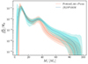 |
Fig. 1. Primary mass differential merger rate density reconstructed with FIGARO along with the POWERLAW+PEAK model from Abbott et al. (2023c). The shaded areas correspond to 68 and 90% credible regions for (H)DPGMM (blue) and POWERLAW+PEAK (orange). |
As (H)DPGMM is meant to reconstruct probability densities, with this specific framework we are not able to estimate the local merger rate density ℛ0: all the distributions are therefore rescaled by this quantity and the y-axis values are not to be taken as indicative of actual values for the differential merger rate. Lastly, concerning Figs. 3a and 4a, due to the way in which they are built, each level has its own vertical linear scale, which may vary significantly within the same plot. By construction, every level is rescaled in such a way that all levels appear to have the same height. We opted for this particular representation because these plots are designed to show the morphological evolution of the differential merger rate rather than the relative magnitude at different redshifts.
2.3. BBH sample
GWTC-3 (Abbott et al. 2023b) adds events detected during the second half of O3 to the already existing GW catalogues, for a total of just below 100 events. Among these observations, Abbott et al. (2023c) use a subset of 62 high-purity BBH events to investigate their astrophysical properties using both astrophysically motivated phenomenological models and semi-parametric models. In the present work, we apply the non-parametric method sketched out in Sect. 2 to the same subset of events in order to be able to compare our findings to the results presented by the LVK collaboration (Abbott et al. 2023c).
3. Results
3.1. Primary mass distribution
Figure 1 shows the marginal primary mass differential merger rate density we obtained with FIGARO applied to the subset of 62 high-purity events from GWTC-3 used in Abbott et al. (2023c). We account for selection effects using a marginalised version of the three-dimensional selection function approximant.
Despite being consistent for the majority of the mass spectrum, our non-parametric model departs from the simpler form of the parametric distribution: the power-law behaviour is present only in the low-mass end of the spectrum (< 25 M⊙) and the smooth tapering of the POWERLAW+PEAK is less pronounced in our reconstruction.
An excess of BHs is visible at around 35 − 40 M⊙, in a region compared with the position of the Gaussian peak of the parametric model (Abbott et al. 2021b, 2023c). However, this excess, with respect to the simple power-law behaviour, is far less localised than the  standard deviation reported in Abbott et al. (2023c), spreading all the way up to ∼70 M⊙. Lastly, the non-parametric distribution shows a cutoff at around 90 M⊙ (mainly due to GW190521, Abbott et al. 2020a).
We made sure that the features we observe – especially the excess between 35 and 70 M⊙ – are not an artefact of the selection function by repeating the analysis with a marginalised version of the two-dimensional (primary and secondary mass) approximant presented in Veske et al. (2021). We find that the features are robust in this respect.
From the mass distribution alone, it is understandably difficult to decide whether the features we find in the BH mass distribution presented in this section are intrinsic or due to stochastic fluctuations; that is, before we even attempt to obtain a reliable interpretation in terms of astrophysical processes. We therefore exploited the possibility made available by (H)DPGMM to infer multivariate probability density to investigate the correlations among the primary mass M1, the mass ratio q, and the redshift z: the presence of such correlations would both confirm the astrophysical origin of the features and guide the development of theoretical models for BH formation channels.
3.2. Joint primary mass, mass ratio, and redshift distribution
In this section, we report and describe the non-parametric reconstruction of the differential merger rate as obtained with FIGARO.
The three-dimensional distribution displayed as a corner plot in Fig. 2 reveals correlations among all the different possible pairs of parameters. In particular, we find the two following aspects to be of particular interest:
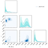 |
Fig. 2. M1, q and z differential merger rate density reconstructed with FIGARO as in Eq. (6). The diagonal panels show the marginal distributions for M1, q and z (top to bottom), respectively, and the panels below diagonal show the median distribution marginalised over the third variable. |
– The mass ratio does not show support for symmetric binaries: this is particularly interesting given that most binary evolution models predict the mass ratio to have a maximum at q ∼ 1 (Dominik et al. 2012; Belczynski et al. 2016; de Mink & Mandel 2016; Giacobbo & Mapelli 2018; Klencki et al. 2018; Broekgaarden et al. 2022). The central panel of Fig. 2 shows a bimodal marginal distribution for the mass ratio, with the main mode centred around q = 0.7. This particular feature is not an artefact of either the model or the code we are employing, as shown in Appendix C.
– The mass distribution evolves with redshift: the lower-left panel of Fig. 2 shows that the primary mass changes with redshift: at high redshift, the mass distribution shows no support for BHs with masses < 20 M⊙. Conversely, for low z, the distribution peaks at around 8 − 10 M⊙ with a cutoff just above 40 M⊙. This is in contrast with the conclusions of Abbott et al. (2021b) and Ray et al. (2023), who do not find evidence for the evolution of the mass distribution; Karathanasis et al. (2023), on the other hand, find indications of such a redshift dependence.
In the following, we describe the different features that are present in the evolving primary mass and mass-ratio distribution, deferring a discussion of these in terms of astrophysical models to Sect. 4.
3.2.1. Mass ratio
Figure 3 shows the evolution with redshift of the mass-ratio differential merger rate, dℛ/dq. Overall, the mass-ratio distribution is roughly constant at all redshifts, and is composed of a single pileup at q ∼ 0.7. The only additional feature is a peak at around q ∼ 0.25 − 0.3 at redshift z ≲ 0.2, populated by two only events (GW190412 and GW190917_114630). This latter feature could simply be due to the small number of events: with more events coming from the current and future observing run, it will be possible to assess its actual significance in the astrophysical distribution.
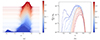 |
Fig. 3. Mass ratio evolution with redshift: joy plot (a) and tomography (b). Both panels report the median distribution only: an animated version of this plot including the 68% credible regions is available online along with plots showing individual slices. This distribution, set aside an excess at low redshifts (z ≲ 0.2), is consistent throughout the whole redshift spectrum in having support at around 0.7, with negligible support for q = 1. |
The differential merger rate in Fig. 3b is not precisely Gaussian: in particular, the distribution favours asymmetric binaries, with a preference for smaller redshifts. Symmetric binaries, conversely, are equally disfavoured independently of the redshift, being suppressed just above q = 0.9 at the 90% credible level (see Fig. 2, second row, second column panel, and online-only material): support for symmetric binaries is almost absent. A more detailed discussion of the shape of this distribution in terms of observed events can be found in Appendix B.
This is in contrast with the parametric model used in Abbott et al. (2023c), where the mass ratio is modelled as a power law: dℛ/dq ∝ qβ, with  . The specific parametric model employed in this analysis inherently favours symmetric binaries, having a maximum at q = 1 for β > 0, potentially making the preference for symmetric systems an ‘artefact’ of the model. Other works making use of semi-parametric models have investigated this distribution (Tiwari 2022; Callister & Farr 2024), but their findings are different from those presented here: Tiwari (2022) made use of a model based on a power law for q (Tiwari 2021), and Edelman et al. (2023) hint at the possibility of a decrease in the merger rate near equal-mass binaries. However, the suppression of symmetric binaries, which is not predicted by the majority of the existing literature on the subject, is confidently found in the data by our non-parametric model.
In order to assess whether or not this feature is an artefact induced by the model we we use, we validated our method using a simulated data set modelled after the findings of Abbott et al. (2023c). The results, presented in Appendix C, show that our model is capable of retrieving the simulated distribution, including a power-law q1.1 for the mass ratio.
3.2.2. Primary mass
The primary mass differential merger rate is reported in Fig. 4. The morphology of the primary mass distribution changes with redshift, from a power-law-like distribution with a preference for low-mass objects at redshift z < 0.4 to a high-mass pileup for z > 0.4. The combination of these two subpopulations, once marginalised over redshift, is the basis for the POWERLAW+PEAK model.
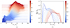 |
Fig. 4. Primary mass evolution with redshift: joy plot (a) and tomography (b). Both panels report the median distribution only: an animated version of this plot including the 68% credible regions is available online along with plots showing individual slices. The mass distribution drastically changes with redshift, suggesting the presence of two distinct populations of BHs. |
Abbott et al. (2023c), in contrast to our findings, find no evidence in favour of a redshift dependence of the primary mass. We ascribe this difference to the parametric model Fishbach et al. (2021), Abbott et al. (2023c) adopted to investigate this correlation: these authors assume that the parameters of the mass distribution change with redshift, rather than allowing for a change in the functional form. In particular, Fishbach et al. (2021), Abbott et al. (2023c) model the high-mass tail of the distribution with a separate power-law index with the cutoff location evolving with redshift. Based on our findings, this model does not properly capture the actual evolution of the mass spectrum. We believe that this is the main reason why Abbott et al. (2023c) do not find evidence in favour of the evolution of the BH mass function with redshift: while performing model selection in the context of Bayesian statistics, the addition of one or more degrees of complexity (such as the second power-law index) that do not improve the modelling of the available data is penalised by the Bayes’ factor.
Given our non-parametric reconstruction, we believe that a good phenomenological parametric model –still based on the POWERLAW+PEAK model– would be a superposition of a power law and a Gaussian peak with a redshift-dependent relative weight w(z), to smoothly transition from the low-redshift, low-mass power law to the high-redshift, high-mass Gaussian peak with a mean that evolves with redshift. When using such a model, a parametric analysis should in principle be able to pick up the redshift evolution of the mass function. van Son et al. (2022) propose a similar model where the relative weights of the power law and the Gaussian peak are proportional to (1 + z)κpl and (1 + z)κpeak, respectively. The authors find marginal evidence in favour of the evolution of the mass with redshift.
3.2.3. Transition from power law to peak
Figure 5 compares the mass distribution in the local Universe, z ≤ 0.2, with a pure power-law distribution with index α = −3.5, as found in Abbott et al. (2023c). This definition of local Universe is purely arbitrary and chosen for visualisation purposes. The non-parametric reconstruction is consistent with the power-law distribution in the 10 ∼ 40 M⊙ region, up to redshift z ∼ 0.13, with cutoffs at both ends of the mass spectrum. At larger redshift, the distribution starts to deviate from the simple power-law behaviour, transitioning towards the ∼35 M⊙ Gaussian-like feature. Given this qualitative agreement between our reconstruction and the power-law reported by Abbott et al. (2023c), we suggest that the POWERLAW+PEAK model is actually driven by the local merger rate density, with a contribution to the Gaussian peak from the BHs further away in look-back time.
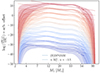 |
Fig. 5. Primary mass conditional differential merger rate density for the local Universe (z ≤ 0.2) compared with a power-law distribution (index α from Abbott et al. 2023c). Shaded areas correspond to 68% credible regions. |
3.2.4. Peak evolution with redshift
Figure 4a shows that the pileup drifts towards larger masses with redshift. This behaviour is highlighted in Fig. 6. We define the peak of the pileup as the maximum of the distribution for6M1 > 25 M⊙. With this, we can isolate three different regimes:
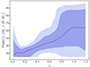 |
Fig. 6. Evolution of the peak of the pileup feature of the mass distribution with redshift. The peak is defined as the maximum of the distribution for M1 > 25 M⊙. The shaded areas correspond to the 68 and 90% credible regions. |
– z < 0.2: this region is dominated by the low-mass power law, and therefore the maximum leans towards 25 M⊙, driven by the preference of the local Universe for lighter BHs. The pileup here, if present, is subdominant.
– 0.2 < z < 0.7: in this redshift interval, the number of available events is large enough to have an accurate reconstruction of the pileup: its peak steadily moves towards larger masses with look-back time, with a somewhat linear dependence.
– z > 0.7: the number of events beyond z = 0.7 is too limited: this fact, combined with the poor resolution of the binary parameters, means that the non-parametric reconstruction provides only a mere hint of the actual behaviour of the underlying distribution. Therefore, the peak in this region is ill defined, and its 90% credible interval encompasses almost the entire mass spectrum.
3.2.5. Minimum and maximum mass of a black hole
Following Abbott et al. (2023c), we define the minimum and maximum mass of a BH as the 1st and 99th percentiles of the mass distribution, M1% and M99%. We report these values in Table 1. The redshift values are the same as those used for the primary mass joy plot. For the same quantities, Abbott et al. (2023c) report  and
and  : both values are in agreement with our findings for the low-redshift region, in which the mass distribution is dominated by the power-law-like feature.
Minimum and maximum value for the BH mass as a function of redshift.
We do not quote the credible interval for M1% for redshifts above 0.25 due to the dominance of selection effects in the low-mass, high-redshift region of the parameter space. The vetted region bounds below the credible interval for this quantity: we deemed the uncertainty estimate for z > 0.25 unreliable, and therefore opted to quote the median value only for reference purposes and to show that a growing trend is nevertheless present.
3.2.6. GW190521: A stand-alone BBH?
The primary mass spectrum also shows a small peak7 at M1 ∼ 90 M⊙, z ∼ 0.8 (see Fig. 7).
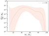 |
Fig. 7. Primary mass conditional differential merger rate density for z = 0.8. The shaded area correspond to the 68% credible region. The peak at M1 ∼ 90 M⊙ marks the presence of GW190521. |
This feature marks the presence of GW190521 (Abbott et al. 2020a), the most massive BBH in the high-purity catalogue considered here, with a total mass of ∼150 M⊙. Abbott et al. (2020b) mention that the primary mass of this BBH is in tension with the population inferred from O1 and O2, suggesting the possibility for this event to be an ‘outlier’. Despite its peculiar component masses, in the latest population studies (most notably Abbott et al. 2021b, 2023c), GW190521 is found to be consistent with the rest of the BBH population. Here, we do not quantitatively assess whether this event is an outlier or not, but rather we use the opportunity to briefly discuss the concept of outliers in the context of non-parametric methods.
An outlier is often defined as a data point that is difficult to explain with or is unlikely to have been produced by a specific population model: this is the case, for example, for a point that has been drawn from a subpopulation not included in the model. However, in the context of a non-parametric analysis, we cannot really talk about outliers in this sense, given that the inferred distribution is the one that best describes all the available data, regardless of their origin. It is up to the analysts to decide whether to include a certain data point (or, in our case, an event) in the data set. An event or a group of events that shows different properties from the rest of the catalogue, in a non-parametric analysis, is simply modelled as a subpopulation on its own, as is also the case for the mass ratio of GW190412 and GW190917_114630. We therefore believe that, in the context of non-parametric analyses, ‘stand-alone’ could be a more appropriate name for such a data point.
GW190521 could, qualitatively, be a stand-alone BBH in this sense, and may be an example of a new, previously unobserved subpopulation of BBHs. This possibility is supported by the results presented by Morton et al. (2023), where we find evidence that GW190521 formed in an AGN disc. In AGN discs, BBHs might form with masses that reach and exceed 100 M⊙ due to the increased probability for hierarchical mergers and accretion (McKernan et al. 2012, 2018; Bellovary et al. 2016; Bartos et al. 2017; Stone et al. 2017; Yang et al. 2019; Tagawa et al. 2020; Gayathri et al. 2022). GW190521 could be the first observed BBH to belong to this subpopulation (Graham et al. 2020).
4. Discussion: Interpretation of the astrophysical distribution
We now discuss the astrophysical implications of the distribution reported in the previous section. In what follows, we assume that the inferred distribution is correct and not affected by the possible caveats discussed above.
4.1. Primary mass
We find that the astrophysical population of BBHs changes with look-back time. Our most significant finding is the morphological evolution of the distribution of primary masses as a function of redshift. In the low-redshift Universe, most BBHs have a primary mass of < 20 M⊙, in agreement with the X-ray binaries in the Milky Way (e.g. Özel et al. 2010; Farr et al. 2011). In contrast, at redshift z ≥ 0.4, the dominant population has a primary mass of ≥20 M⊙.
This evolution of the primary mass with redshift has several possible, non-mutually exclusive interpretations. First, we can think of a metallicity trend: in the low-redshift Universe, we expect to observe mostly BBHs born from metal-rich progenitors, whereas, in the high-redshift Universe, most BBHs should originate from metal-poor (Z ≤ 10−4) and metal-free progenitors (Hartwig et al. 2016; Kinugawa et al. 2016; Inayoshi et al. 2017; Mapelli et al. 2017; Schneider et al. 2017; Tanikawa et al. 2021b; Costa et al. 2023). The primary mass of BBHs born from metal-rich stars is expected to peak at ∼8 − 12 M⊙, because of efficient wind mass loss (Belczynski et al. 2016; Stevenson et al. 2017; Giacobbo & Mapelli 2018; Klencki et al. 2018; Kruckow et al. 2018; Spera et al. 2019; Schneider et al. 2021; Iorio et al. 2023; Fragos et al. 2023; Agrawal et al. 2023). Conversely, the low-mass peak of the primary mass function is suppressed in BBHs born from metal-poor and metal-free stars (see e.g. Fig. 8 of Santoliquido et al. 2023): most of them have primary mass in the ∼20 − 50 M⊙ range, possibly enforcing the peak at ∼35 M⊙ (Kinugawa et al. 2014, 2020; Liu & Bromm 2020; Tanikawa et al. 2021a, 2022; Vink et al. 2021; Costa et al. 2023; Santoliquido et al. 2023). However, current models do not predict that the low-mass peak has already disappeared at z ∼ 0.4, but rather at higher redshift (z ≥ 6, Santoliquido et al. 2023).
A second possible interpretation for the evolution of the primary mass function is a change of the relative importance of different formation channels with redshift. For example, the dominant formation channel might change from isolated binary evolution to dynamical assembly as redshift increases. Several previous studies indicate that we expect higher BBH masses from dynamical formation in dense star clusters (e.g. Rodriguez et al. 2016a; Askar et al. 2017; Chatterjee et al. 2017; Antonini et al. 2019, 2023; Kremer et al. 2020; Torniamenti et al. 2022) and AGN discs (e.g. McKernan et al. 2012, 2018; Bellovary et al. 2016; Bartos et al. 2017; Stone et al. 2017; Tagawa et al. 2020). In particular, globular cluster formation peaks at a redshift of z ∼ 3 − 4 (VandenBerg et al. 2013; Choksi et al. 2018; El-Badry et al. 2019). This redshift-dependent formation history, combined with longer-than-expected delay times and/or a higher-than-expected merger efficiency, might produce a dominant population of massive BH mergers down to a redshift of z ∼ 0.4 (Rodriguez & Loeb 2018; Choksi et al. 2019; Antonini & Gieles 2020; Antonini et al. 2023; Mapelli et al. 2022).
If this interpretation is correct, we should observe an evolution with redshift not only of the primary mass function but also of the effective and precessing spin parameters. Furthermore, dynamical interactions randomise the orientation of BH spins, leading to a nearly isotropic spin distribution, while isolated binary evolution tends to align BH spins with the orbital angular momentum of the binary systems (e.g. Kalogera 2000; Rodriguez et al. 2016b). Moreover, hierarchical BBH mergers are associated with large spin magnitudes, at least for the primary BH, because the dimensionless spins of merger remnants peak at ∼0.7 (Buonanno et al. 2008; Jiménez-Forteza et al. 2017). Therefore, an increase in the hierarchical merger population with redshift would result in a broadening of the effective spin distribution with redshift, and would lead to the emergence of a peak in the precessing spin around ∼0.7 (Baibhav et al. 2020; Mapelli et al. 2021). The selection function implementation used in the present work does not account for spin, and therefore we did not include these parameters in this work. We plan to investigate the effective spin distribution in a future paper. Here, we mention that Biscoveanu et al. (2022) find an increase in the width of the effective spin distribution of BBHs with increasing redshift. This might suggest a larger contribution of the hierarchical merger scenario at higher redshift (Baibhav et al. 2020; Mapelli et al. 2021); kritos:2022; (Santini et al. 2023), but it is still consistent with other scenarios.
A third hypothesis (not necessarily alternative to the other two) is that the evolution of the primary mass function captured by our method stems from processes that current models fail to properly describe. Overall, models that do not predict any evolution (or predict only a mild evolution) with redshift (e.g. Mapelli et al. 2019) are already challenged by our findings.
4.2. Mass ratio
Our results seem to indicate that the preferred BBH mass ratio is q ∼ 0.7, with little or no evolution with redshift (with the exception of the lowest redshift region, dominated by the events GW190412 and GW190917_114630). In contrast, most current models (especially isolated binary evolution via common envelope and chemically homogeneous evolution) indicate a preference for equal-mass or nearly equal-mass systems (e.g. Belczynski et al. 2016; de Mink & Mandel 2016; Giacobbo & Mapelli 2018; Klencki et al. 2018; Kruckow et al. 2018; Broekgaarden et al. 2022), with a few exceptions (van Son et al. 2022; Santoliquido et al. 2023).
Most dynamical formation channels allow a larger fraction of unequal-mass systems than isolated binary evolution (e.g. Di Carlo et al. 2019; Arca Sedda et al. 2020; Torniamenti et al. 2022). In particular, BBHs born from hierarchical mergers have a strong preference for unequal-mass mergers (Rodriguez et al. 2019; Fragione & Silk 2020; Zevin & Holz 2022). However, recent studies show that hierarchical mergers cannot account for the majority of LVK events (Zevin & Holz 2022; Fishbach et al. 2022).
Recently, Santoliquido et al. (2023) showed that metal-poor and metal-free BBH mergers tend to have q ∼ 0.7 at redshift z ≲ 5 (see their Fig. 7). This feature is mostly an effect of the evolutionary channel: in the models of these latter authors, all the BBHs with q ≤ 0.7 form from binary systems in which the progenitor star of the primary BH retains at least a fraction of its H-rich envelope at the time it collapses to a BH. In most cases, the binary system evolves via stable mass transfer. Similarly, van Son et al. (2022) find that BBHs formed via stable mass transfer in binary systems peak at q ∼ 0.6 − 0.7 (see their Fig. 9). Notably, the revised treatment of Roche-lobe overflow stability by Olejak et al. (2021) leads to significantly lower values of q ∼ 0.4 − 0.6 (see their Fig. 4): most of the unequal-mass BBHs in their model form without common-envelope evolution. Clues in this direction are also reported in Gallegos-Garcia et al. (2021).
Overall, none of the current models in the literature are able to explain the non-evolving mass ratio q ∼ 0.7 in conjunction with rapid evolution of the primary mass with redshift that we find with (H)DPGMM. This might indicate that astrophysical models fail to describe some key physical process, such as the efficiency of mass accretion and angular momentum transport during mass transfer (e.g. Gallegos-Garcia et al. 2023; Willcox et al. 2023), the impact of stellar rotation (e.g. Mapelli et al. 2020; Marchant & Moriya 2020; Riley et al. 2021), or the efficiency of dynamical assembly (e.g. Fragione & Kocsis 2018; Mapelli et al. 2022).
5. Conclusions
We applied our non-parametric model, (H)DPGMM, to the GW events included in GWTC-3, focusing on the distribution of primary mass, mass ratio, and redshift. This distribution, once corrected for selection effects, clearly exhibits a correlation among the three parameters, providing support in favour of the evolution of the primary mass distribution with redshift. Our main findings can be summarised as follows:
-
The mass-ratio distribution does not show support for symmetric binaries, favouring systems with q ∼ 0.7, mostly independent of redshift.
-
The primary mass distribution is composed of two distinct subpopulations: a low-mass, low-redshift power-law-like population and a high-mass, high-redshift Gaussian-like feature. The change between the two subpopulations happens between z ∼ 0.2 and z ∼ 0.4.
-
The position of the Gaussian-like feature evolves with redshift, drifting towards larger masses with look-back time.
We outline two possible non-mutually exclusive explanations for the evolution of the astrophysical BBH population with look-back time. The mass could follow a trend in metallicity, changing from low-mass BHs born from metal-rich progenitor stars at low redshift to more massive BHs produced by metal-poor and metal-rich stars. The other possible interpretation is that there is a change in the relative importance of different formation channels, from an isolated evolution-dominated scenario at z < 0.4 to a prevalent contribution of dynamically assembled systems for z > 0.4.
Our findings for the mass ratio are in contrast with most of the current models for isolated binary evolution, where the favoured systems are symmetric or near-symmetric binaries; unequal-mass systems are more likely to be produced by dynamical formation channels or hierarchical mergers. The apparent contradiction between the rapid evolution of the BH mass function and the constancy of the mass-ratio distribution may suggest that there is some missing physics in the present astrophysical models.
The results presented in this paper will be crucial not only for the advancement of BH astrophysics, but also for all those investigations that, to a greater or lesser extent, rely on the BH mass distribution. For example, the mass function is a key ingredient of methods for the inference of cosmological parameters (Abbott 2023a), the galaxy catalogue method (Gray et al. 2020), and the joint population and cosmology approach (Mastrogiovanni et al. 2021). Moreover, the presence of non-scale-invariant and redshift-evolving features, such as the pileup at z > 0.4, will have a dramatic impact on methods that rely on features in the mass distribution to infer cosmological parameters (Farr et al. 2019; Mancarella et al. 2022; Mukherjee 2022).
As a final remark, we reiterate that there are two important caveats to the findings presented in this paper, namely the data are representative of the underlying population (the data used here are not censored and the features in the underlying distribution are properly sampled) and the approximant we employed captures all the features of the selection function. We made sure that these assumptions are met (see Appendices A, C and D). Nonetheless, it is still possible that some of the features we report are to be ascribed to the limited number of available GW events: the new events detected during the ongoing LVK run, together with the capacity of data-driven models such as (H)DPGMM to automatically include new features, will either confirm or disprove the findings reported in this paper and will unveil new features of the BH population.
Movies
Movie 1 associated with Fig. 3 (slices_q_log) Access here
Movie 2 associated with Fig. 3 (slices_q) Access here
Movie 3 associated with Fig. 4 (slices_m1_log) Access here
Movie 4 associated with Fig. 4 (slices_m1) Access here
While dealing with parameters with boundaries, such as q, we make use of the parametrisation presented in Rinaldi & Del Pozzo (2022a), Sect. 3.1., for each parameter separately.
FIGARO is publicly available at https://github.com/sterinaldi/FIGARO.
Again, we follow the same convention as Rinaldi & Del Pozzo (2022a), where ‘astrophysical distribution’ refers to the that from which the observed events are drawn before accounting for selection effects.
The code to evaluate our pdet model and fit its parameters to injection results, and the resulting maximum likelihood parameter values, are publicly available at https://github.com/AnaLorenzoMedina/cbc_pdet.
Acknowledgments
The authors are grateful to Christopher Moore, Thomas Callister and the anonymous referee for useful comments. We are also thankful to the organisers and participants of GWPopNext (University of Milano-Bicocca, July 2023) for stimulating discussion. M.M. acknowledges financial support from the European Research Council for the ERC Consolidator grant DEMOBLACK, under contract no. 770017, and from the German Excellence Strategy via the Heidelberg Cluster of Excellence (EXC 2181 – 390900948) STRUCTURES. This work has received financial support from Xunta de Galicia (CIGUS Network of research centers) and by European Union ERDF. A.L.M. and T.D. are supported by research grant PID2020-118635GB-I00 from the Spanish Ministerio de Ciencia e Innovación. This research has made use of data or software obtained from the Gravitational Wave Open Science Center (https://www.gwosc.org/), a service of the LIGO Scientific Collaboration, the Virgo Collaboration, and KAGRA. This material is based upon work supported by NSF’s LIGO Laboratory which is a major facility fully funded by the National Science Foundation, as well as the Science and Technology Facilities Council (STFC) of the United Kingdom, the Max-Planck-Society (MPS), and the State of Niedersachsen/Germany for support of the construction of Advanced LIGO and construction and operation of the GEO600 detector. Additional support for Advanced LIGO was provided by the Australian Research Council. Virgo is funded, through the European Gravitational Observatory (EGO), by the French Centre National de Recherche Scientifique (CNRS), the Italian Istituto Nazionale di Fisica Nucleare (INFN) and the Dutch Nikhef, with contributions by institutions from Belgium, Germany, Greece, Hungary, Ireland, Japan, Monaco, Poland, Portugal, Spain. KAGRA is supported by Ministry of Education, Culture, Sports, Science and Technology (MEXT), Japan Society for the Promotion of Science (JSPS) in Japan; National Research Foundation (NRF) and Ministry of Science and ICT (MSIT) in Korea; Academia Sinica (AS) and National Science and Technology Council (NSTC) in Taiwan.
References
- Aasi, J., Abbott, B. P., Abbott, R., et al. 2015, CQG, 32, 074001 [Google Scholar]
- Abbott, B. P., Abbott, R., Abbott, T. D., et al. 2016a, Phys. Rev. Lett., 116, 061102 [Google Scholar]
- Abbott, B. P., Abbott, R., Abbott, T. D., et al. 2016b, Phys. Rev. Lett., 116, 241102 [NASA ADS] [CrossRef] [Google Scholar]
- Abbott, B. P., Abbott, R., Abbott, T. D., et al. 2019, ApJ, 882, L24 [Google Scholar]
- Abbott, R., Abbott, T. D., Abraham, S., et al. 2020a, Phys. Rev. Lett., 125, 101102 [Google Scholar]
- Abbott, R., Abbott, T. D., Abraham, S., et al. 2020b, ApJ, 900, L13 [NASA ADS] [CrossRef] [Google Scholar]
- Abbott, R., Abbott, T. D., Abraham, S., et al. 2021a, Phys. Rev. X, 11, 021053 [Google Scholar]
- Abbott, R., Abbott, T. D., Abraham, S., et al. 2021b, ApJ, 913, L7 [NASA ADS] [CrossRef] [Google Scholar]
- Abbott, R., Abe, H., Acernese, F., et al. 2023a, ApJ, 949, 76 [NASA ADS] [CrossRef] [Google Scholar]
- Abbott, R., Abbott, T. D., Acernese, F., et al. 2023b, Phys. Rev. X, 13, 041039 [Google Scholar]
- Abbott, R., Abbott, T. D., Acernese, F., et al. 2023c, Phys. Rev. X, 13, 011048 [NASA ADS] [Google Scholar]
- Abbott, R., Abbott, T. D., Acernese, F., et al. 2024, Phys. Rev. D, 109, 022001 [NASA ADS] [CrossRef] [Google Scholar]
- Acernese, F., Agathos, M., Agatsuma, K., et al. 2015, CQG, 32, 024001 [NASA ADS] [CrossRef] [Google Scholar]
- Adamcewicz, C., Lasky, P. D., & Thrane, E. 2023, ApJ, 958, 13 [NASA ADS] [CrossRef] [Google Scholar]
- Agrawal, P., Hurley, J., Stevenson, S., et al. 2023, MNRAS, 525, 933 [NASA ADS] [CrossRef] [Google Scholar]
- Akutsu, T., Ando, M., Arai, K., et al. 2020, Prog. Theor. Exp. Phys., 2021, 05A101 [CrossRef] [Google Scholar]
- Antonini, F., & Gieles, M. 2020, MNRAS, 492, 2936 [CrossRef] [Google Scholar]
- Antonini, F., Gieles, M., & Gualandris, A. 2019, MNRAS, 486, 5008 [NASA ADS] [CrossRef] [Google Scholar]
- Antonini, F., Gieles, M., Dosopoulou, F., & Chattopadhyay, D. 2023, MNRAS, 522, 466 [NASA ADS] [CrossRef] [Google Scholar]
- Arca Sedda, M., Mapelli, M., Spera, M., Benacquista, M., & Giacobbo, N. 2020, ApJ, 894, 133 [NASA ADS] [CrossRef] [Google Scholar]
- Arca Sedda, M., Li, G., & Kocsis, B. 2021, A&A, 650, A189 [NASA ADS] [CrossRef] [EDP Sciences] [Google Scholar]
- Askar, A., Szkudlarek, M., Gondek-Rosińska, D., Giersz, M., & Bulik, T. 2017, MNRAS, 464, L36 [CrossRef] [Google Scholar]
- Aso, Y., Michimura, Y., Somiya, K., et al. 2013, Phys. Rev. D, 88, 043007 [NASA ADS] [CrossRef] [Google Scholar]
- Bahcall, J. N. 1978, in Physics and Astrophysics of Neutron Stars and Black Holes, eds. R. Giacconi, & R. Ruffini, 63 [Google Scholar]
- Baibhav, V., Gerosa, D., Berti, E., et al. 2020, Phys. Rev. D, 102, 043002 [NASA ADS] [CrossRef] [Google Scholar]
- Banerjee, S. 2018, MNRAS, 473, 909 [CrossRef] [Google Scholar]
- Banerjee, S., Baumgardt, H., & Kroupa, P. 2010, MNRAS, 402, 371 [Google Scholar]
- Bartos, I., Kocsis, B., Haiman, Z., & Márka, S. 2017, ApJ, 835, 165 [Google Scholar]
- Belczynski, K., Kalogera, V., & Bulik, T. 2002, ApJ, 572, 407 [NASA ADS] [CrossRef] [Google Scholar]
- Belczynski, K., Bulik, T., Fryer, C. L., et al. 2010, ApJ, 714, 1217 [NASA ADS] [CrossRef] [Google Scholar]
- Belczynski, K., Holz, D. E., Bulik, T., & O’Shaughnessy, R. 2016, Nature, 534, 512 [NASA ADS] [CrossRef] [Google Scholar]
- Bellovary, J. M., Mac Low, M.-M., McKernan, B., & Ford, K. E. S. 2016, ApJ, 819, L17 [NASA ADS] [CrossRef] [Google Scholar]
- Bethe, H. A., & Brown, G. E. 1998, ApJ, 506, 780 [Google Scholar]
- Biscoveanu, S., Callister, T. A., Haster, C.-J., et al. 2022, ApJ, 932, L19 [NASA ADS] [CrossRef] [Google Scholar]
- Bouffanais, Y., Mapelli, M., Santoliquido, F., et al. 2021, MNRAS, 507, 5224 [NASA ADS] [CrossRef] [Google Scholar]
- Briel, M. M., Stevance, H. F., & Eldridge, J. J. 2023, MNRAS, 520, 5724 [Google Scholar]
- Broekgaarden, F. S., Berger, E., Stevenson, S., et al. 2022, MNRAS, 516, 5737 [NASA ADS] [CrossRef] [Google Scholar]
- Buonanno, A., Kidder, L. E., & Lehner, L. 2008, Phys. Rev. D, 77, 026004 [CrossRef] [Google Scholar]
- Byram, E. T., Chubb, T. A., & Friedman, H. 1966, AJ, 71, 379 [NASA ADS] [CrossRef] [Google Scholar]
- Callister, T. A., & Farr, W. M. 2024, Phys. Rev. X, 14, 021005 [NASA ADS] [Google Scholar]
- Callister, T. A., Haster, C.-J., Ng, K. K. Y., Vitale, S., & Farr, W. M. 2021, ApJ, 922, L5 [NASA ADS] [CrossRef] [Google Scholar]
- Carr, B. J. 1975, ApJ, 201, 1 [NASA ADS] [CrossRef] [Google Scholar]
- Chatterjee, S., Rodriguez, C. L., & Rasio, F. A. 2017, ApJ, 834, 68 [NASA ADS] [CrossRef] [Google Scholar]
- Choksi, N., Gnedin, O. Y., & Li, H. 2018, MNRAS, 480, 2343 [NASA ADS] [CrossRef] [Google Scholar]
- Choksi, N., Volonteri, M., Colpi, M., Gnedin, O. Y., & Li, H. 2019, ApJ, 873, 100 [NASA ADS] [CrossRef] [Google Scholar]
- Costa, G., Mapelli, M., Iorio, G., et al. 2023, MNRAS, 525, 2891 [NASA ADS] [CrossRef] [Google Scholar]
- Dall’Amico, M., Mapelli, M., Di Carlo, U. N., et al. 2021, MNRAS, 508, 3045 [CrossRef] [Google Scholar]
- de Mink, S. E., & Mandel, I. 2016, MNRAS, 460, 3545 [NASA ADS] [CrossRef] [Google Scholar]
- Di Carlo, U. N., Giacobbo, N., Mapelli, M., et al. 2019, MNRAS, 487, 2947 [NASA ADS] [CrossRef] [Google Scholar]
- Di Carlo, U. N., Mapelli, M., Giacobbo, N., et al. 2020, MNRAS, 498, 495 [NASA ADS] [CrossRef] [Google Scholar]
- Dominik, M., Belczynski, K., Fryer, C., et al. 2012, ApJ, 759, 52 [Google Scholar]
- Edelman, B., Rivera-Paleo, F. J., Merritt, J. D., et al. 2021, Phys. Rev. D, 103, 042004 [CrossRef] [Google Scholar]
- Edelman, B., Farr, B., & Doctor, Z. 2023, ApJ, 946, 16 [NASA ADS] [CrossRef] [Google Scholar]
- El-Badry, K., Quataert, E., Weisz, D. R., Choksi, N., & Boylan-Kolchin, M. 2019, MNRAS, 482, 4528 [Google Scholar]
- Eldridge, J. J., & Stanway, E. R. 2016, MNRAS, 462, 3302 [Google Scholar]
- Essick, R. 2021, Res. Notes AAS, 5, 220 [NASA ADS] [CrossRef] [Google Scholar]
- Essick, R., & Fishbach, M. 2024, ApJ, 962, 169 [NASA ADS] [CrossRef] [Google Scholar]
- Farr, W. M. 2019, Res. Notes AAS, 3, 66 [NASA ADS] [CrossRef] [Google Scholar]
- Farr, W. M., Sravan, N., Cantrell, A., et al. 2011, ApJ, 741, 103 [NASA ADS] [CrossRef] [Google Scholar]
- Farr, W. M., Fishbach, M., Ye, J., & Holz, D. E. 2019, ApJ, 883, L42 [NASA ADS] [CrossRef] [Google Scholar]
- Finn, L. S., & Chernoff, D. F. 1993, Phys. Rev. D, 47, 2198 [NASA ADS] [CrossRef] [Google Scholar]
- Fishbach, M., & Holz, D. E. 2017, ApJ, 851, L25 [NASA ADS] [CrossRef] [Google Scholar]
- Fishbach, M., Holz, D. E., & Farr, B. 2017, ApJ, 840, L24 [NASA ADS] [CrossRef] [Google Scholar]
- Fishbach, M., Doctor, Z., Callister, T., et al. 2021, ApJ, 912, 98 [NASA ADS] [CrossRef] [Google Scholar]
- Fishbach, M., Kimball, C., & Kalogera, V. 2022, ApJ, 935, L26 [NASA ADS] [CrossRef] [Google Scholar]
- Fragione, G., & Kocsis, B. 2018, Phys. Rev. Lett., 121, 161103 [Google Scholar]
- Fragione, G., & Rasio, F. A. 2023, ApJ, 951, 129 [NASA ADS] [CrossRef] [Google Scholar]
- Fragione, G., & Silk, J. 2020, MNRAS, 498, 4591 [NASA ADS] [CrossRef] [Google Scholar]
- Fragos, T., Andrews, J. J., Bavera, S. S., et al. 2023, ApJS, 264, 45 [NASA ADS] [CrossRef] [Google Scholar]
- Fryer, C. L., Belczynski, K., Wiktorowicz, G., et al. 2012, ApJ, 749, 91 [Google Scholar]
- Galaudage, S., Talbot, C., Nagar, T., et al. 2021, ApJ, 921, L15 [NASA ADS] [CrossRef] [Google Scholar]
- Gallegos-Garcia, M., Berry, C. P. L., Marchant, P., & Kalogera, V. 2021, ApJ, 922, 110 [NASA ADS] [CrossRef] [Google Scholar]
- Gallegos-Garcia, M., Jacquemin-Ide, J., & Kalogera, V. 2023, ApJ, submitted, [arXiv:2308.13146] [Google Scholar]
- Gayathri, V., Healy, J., Lange, J., et al. 2022, Nat. Astron., 6, 344 [NASA ADS] [CrossRef] [Google Scholar]
- Gerosa, D., & Berti, E. 2017, Phys. Rev. D, 95, 124046 [NASA ADS] [CrossRef] [Google Scholar]
- Gerosa, D., & Fishbach, M. 2021, Nat. Astron., 5, 749 [NASA ADS] [CrossRef] [Google Scholar]
- Giacobbo, N., & Mapelli, M. 2018, MNRAS, 480, 2011 [Google Scholar]
- Graham, M. J., Ford, K. E. S., McKernan, B., et al. 2020, Phys. Rev. Lett., 124, 251102 [NASA ADS] [CrossRef] [Google Scholar]
- Gray, R., Hernandez, I. M., Qi, H., et al. 2020, Phys. Rev. D, 101, 122001 [NASA ADS] [CrossRef] [Google Scholar]
- Hartwig, T., Volonteri, M., Bromm, V., et al. 2016, MNRAS, 460, L74 [NASA ADS] [CrossRef] [Google Scholar]
- Heger, A., Fryer, C. L., Woosley, S. E., Langer, N., & Hartmann, D. H. 2003, ApJ, 591, 288 [CrossRef] [Google Scholar]
- Hurley, J. R., Tout, C. A., & Pols, O. R. 2002, MNRAS, 329, 897 [Google Scholar]
- Inayoshi, K., Hirai, R., Kinugawa, T., & Hotokezaka, K. 2017, MNRAS, 468, 5020 [Google Scholar]
- Iorio, G., Mapelli, M., Costa, G., et al. 2023, MNRAS, 524, 426 [NASA ADS] [CrossRef] [Google Scholar]
- Iyer, B., Souradeep, T., Unnikrishnan, C., et al. 2011, LIGO-India, Proposal of the Consortium for Indian Initiative in Gravitational-wave Observations (IndIGO), https://dcc.ligo.org/LIGO-M1100296/public [Google Scholar]
- Jiménez-Forteza, X., Keitel, D., Husa, S., et al. 2017, Phys. Rev. D, 95, 064024 [CrossRef] [Google Scholar]
- Kalogera, V. 2000, ApJ, 541, 319 [NASA ADS] [CrossRef] [Google Scholar]
- Karathanasis, C., Mukherjee, S., & Mastrogiovanni, S. 2023, MNRAS, 523, 4539 [NASA ADS] [Google Scholar]
- Kimball, C., Talbot, C., Berry, C. P. L., et al. 2021, ApJ, 915, L35 [CrossRef] [Google Scholar]
- Kinugawa, T., Inayoshi, K., Hotokezaka, K., Nakauchi, D., & Nakamura, T. 2014, MNRAS, 442, 2963 [NASA ADS] [CrossRef] [Google Scholar]
- Kinugawa, T., Miyamoto, A., Kanda, N., & Nakamura, T. 2016, MNRAS, 456, 1093 [CrossRef] [Google Scholar]
- Kinugawa, T., Nakamura, T., & Nakano, H. 2020, MNRAS, 498, 3946 [NASA ADS] [CrossRef] [Google Scholar]
- Klencki, J., Moe, M., Gladysz, W., et al. 2018, A&A, 619, A77 [NASA ADS] [CrossRef] [EDP Sciences] [Google Scholar]
- Kremer, K., Ye, C. S., Rui, N. Z., et al. 2020, ApJS, 247, 48 [NASA ADS] [CrossRef] [Google Scholar]
- Kritos, K., Strokov, V., Baibhav, V., & Berti, E. 2022, arXiv e-prints [arXiv:2210.10055] [Google Scholar]
- Kroupa, P. 2001, in Dynamics of Star Clusters and the Milky Way, eds. S. Deiters, B. Fuchs, A. Just, R. Spurzem, & R. Wielen, ASP Conf. Ser., 228, 187 [NASA ADS] [Google Scholar]
- Kruckow, M. U., Tauris, T. M., Langer, N., Kramer, M., & Izzard, R. G. 2018, MNRAS, 481, 1908 [CrossRef] [Google Scholar]
- Kumamoto, J., Fujii, M. S., & Tanikawa, A. 2020, MNRAS, 495, 4268 [Google Scholar]
- Lamers, H. J., & Levesque, E. M. 2017, Understanding Stellar Evolution (IOP Publishing), 2514 [Google Scholar]
- Li, Y.-J., Wang, Y.-Z., Han, M.-Z., et al. 2021a, ApJ, 917, 33 [NASA ADS] [CrossRef] [Google Scholar]
- Li, Y.-P., Dempsey, A. M., Li, S., Li, H., & Li, J. 2021b, ApJ, 911, 124 [NASA ADS] [CrossRef] [Google Scholar]
- Liu, B., & Bromm, V. 2020, ApJ, 903, L40 [NASA ADS] [CrossRef] [Google Scholar]
- LIGO Scientific Collaboration, Virgo Collaboration, & KAGRA Collaboration 2023, https://doi.org/10.5281/zenodo.7890437 [Google Scholar]
- Loredo, T. J. 2004, in Bayesian Inference and Maximum Entropy Methods in Science and Engineering: 24th International Workshop on Bayesian Inference and Maximum Entropy Methods in Science and Engineering, eds. R. Fischer, R. Preuss, & U. V. Toussaint, AIP Conf. Ser., 735, 195 [NASA ADS] [CrossRef] [Google Scholar]
- Mancarella, M., Genoud-Prachex, E., & Maggiore, M. 2022, Phys. Rev. D, 105, 064030 [NASA ADS] [CrossRef] [Google Scholar]
- Mandel, I., Farr, W. M., Colonna, A., et al. 2016, MNRAS, 465, 3254 [Google Scholar]
- Mandel, I., Farr, W. M., & Gair, J. R. 2019, MNRAS, 486, 1086 [Google Scholar]
- Mapelli, M. 2016, MNRAS, 459, 3432 [NASA ADS] [CrossRef] [Google Scholar]
- Mapelli, M., Colpi, M., & Zampieri, L. 2009, MNRAS, 395, L71 [NASA ADS] [CrossRef] [Google Scholar]
- Mapelli, M., Ripamonti, E., Zampieri, L., Colpi, M., & Bressan, A. 2010, MNRAS, 408, 234 [NASA ADS] [CrossRef] [Google Scholar]
- Mapelli, M., Giacobbo, N., Ripamonti, E., & Spera, M. 2017, MNRAS, 472, 2422 [NASA ADS] [CrossRef] [Google Scholar]
- Mapelli, M., Giacobbo, N., Santoliquido, F., & Artale, M. C. 2019, MNRAS, 487, 2 [NASA ADS] [CrossRef] [Google Scholar]
- Mapelli, M., Spera, M., Montanari, E., et al. 2020, ApJ, 888, 76 [NASA ADS] [CrossRef] [Google Scholar]
- Mapelli, M., Dall’Amico, M., Bouffanais, Y., et al. 2021, MNRAS, 505, 339 [CrossRef] [Google Scholar]
- Mapelli, M., Bouffanais, Y., Santoliquido, F., Arca Sedda, M., & Artale, M. C. 2022, MNRAS, 511, 5797 [NASA ADS] [CrossRef] [Google Scholar]
- Marchant, P., & Moriya, T. J. 2020, A&A, 640, L18 [EDP Sciences] [Google Scholar]
- Mastrogiovanni, S., Leyde, K., Karathanasis, C., et al. 2021, Phys. Rev. D, 104, 062009 [NASA ADS] [CrossRef] [Google Scholar]
- McKernan, B., Ford, K. E. S., Lyra, W., & Perets, H. B. 2012, MNRAS, 425, 460 [NASA ADS] [CrossRef] [Google Scholar]
- McKernan, B., Ford, K. E. S., Bellovary, J., et al. 2018, ApJ, 866, 66 [Google Scholar]
- Miller, M. C., & Hamilton, D. P. 2002, MNRAS, 330, 232 [Google Scholar]
- Morton, S. L., Rinaldi, S., Torres-Orjuela, A., et al. 2023, Phys. Rev. D, 108, 123039 [NASA ADS] [CrossRef] [Google Scholar]
- Mould, M., Gerosa, D., & Taylor, S. R. 2022, Phys. Rev. D, 106, 103013 [NASA ADS] [CrossRef] [Google Scholar]
- Mukherjee, S. 2022, MNRAS, 515, 5495 [NASA ADS] [CrossRef] [Google Scholar]
- Nguyen, T. T., Nguyen, H. D., Chamroukhi, F., & McLachlan, G. J. 2020, Cog. Math. St., 7, 1750861 [CrossRef] [Google Scholar]
- Olejak, A., Belczynski, K., & Ivanova, N. 2021, A&A, 651, A100 [NASA ADS] [CrossRef] [EDP Sciences] [Google Scholar]
- Özel, F., Psaltis, D., Narayan, R., & McClintock, J. E. 2010, ApJ, 725, 1918 [CrossRef] [Google Scholar]
- Planck Collaboration VI. 2020, A&A, 641, A6 [NASA ADS] [CrossRef] [EDP Sciences] [Google Scholar]
- Portegies Zwart, S. F., & McMillan, S. L. W. 2000, ApJ, 528, L17 [Google Scholar]
- Ray, A., Magaña Hernandez, I., Mohite, S., Creighton, J., & Kapadia, S. 2023, ApJ, 957, 37 [NASA ADS] [CrossRef] [Google Scholar]
- Riley, J., Mandel, I., Marchant, P., et al. 2021, MNRAS, 505, 663 [Google Scholar]
- Rinaldi, S., & Del Pozzo, W. 2022a, MNRAS, 509, 5454 [Google Scholar]
- Rinaldi, S., & Del Pozzo, W. 2022b, MNRAS, 517, L5 [NASA ADS] [CrossRef] [Google Scholar]
- Rodriguez, C. 2023, in AAS/High Energy Astrophysics Division, Vol. 55, AAS/High Energy Astrophysics Division, 115.18 [Google Scholar]
- Rodriguez, C. L., & Loeb, A. 2018, ApJ, 866, L5 [NASA ADS] [CrossRef] [Google Scholar]
- Rodriguez, C. L., Chatterjee, S., & Rasio, F. A. 2016a, Phys. Rev. D, 93, 084029 [NASA ADS] [CrossRef] [Google Scholar]
- Rodriguez, C. L., Zevin, M., Pankow, C., Kalogera, V., & Rasio, F. A. 2016b, ApJ, 832, L2 [NASA ADS] [CrossRef] [Google Scholar]
- Rodriguez, C. L., Zevin, M., Amaro-Seoane, P., et al. 2019, Phys. Rev. D, 100, 043027 [Google Scholar]
- Romero-Shaw, I., Lasky, P. D., & Thrane, E. 2022, ApJ, 940, 171 [CrossRef] [Google Scholar]
- Roulet, J., Chia, H. S., Olsen, S., et al. 2021, Phys. Rev. D, 104, 083010 [NASA ADS] [CrossRef] [Google Scholar]
- Sadiq, J., Dent, T., & Gieles, M. 2024, ApJ, 960, 65 [NASA ADS] [CrossRef] [Google Scholar]
- Salpeter, E. E. 1955, ApJ, 121, 161 [Google Scholar]
- Samsing, J. 2018, Phys. Rev. D, 97, 103014 [CrossRef] [Google Scholar]
- Samsing, J., Bartos, I., D’Orazio, D. J., et al. 2022, Nature, 603, 237 [NASA ADS] [CrossRef] [Google Scholar]
- Santini, A., Gerosa, D., Cotesta, R., & Berti, E. 2023, Phys. Rev. D, 108, 083033 [CrossRef] [Google Scholar]
- Santoliquido, F., Mapelli, M., Iorio, G., et al. 2023, MNRAS, 524, 307 [NASA ADS] [CrossRef] [Google Scholar]
- Schneider, R., Graziani, L., Marassi, S., et al. 2017, MNRAS, 471, L105 [NASA ADS] [CrossRef] [Google Scholar]
- Schneider, F. R. N., Podsiadlowski, P., & Müller, B. 2021, A&A, 645, A5 [NASA ADS] [CrossRef] [EDP Sciences] [Google Scholar]
- Spera, M., Mapelli, M., Giacobbo, N., et al. 2019, MNRAS, 485, 889 [Google Scholar]
- Srinivasan, R., Lamberts, A., Bizouard, M. A., Bruel, T., & Mastrogiovanni, S. 2023, MNRAS, 524, 60 [CrossRef] [Google Scholar]
- Stevenson, S., & Clarke, T. A. 2022, MNRAS, 517, 4034 [Google Scholar]
- Stevenson, S., Vigna-Gómez, A., Mandel, I., et al. 2017, Nat. Commun., 8, 14906 [Google Scholar]
- Stevenson, S., Sampson, M., Powell, J., et al. 2019, ApJ, 882, 121 [Google Scholar]
- Stone, N. C., Metzger, B. D., & Haiman, Z. 2017, MNRAS, 464, 946 [Google Scholar]
- Tagawa, H., Haiman, Z., & Kocsis, B. 2020, ApJ, 898, 25 [NASA ADS] [CrossRef] [Google Scholar]
- Tagawa, H., Kocsis, B., Haiman, Z., et al. 2021, ApJ, 908, 194 [NASA ADS] [CrossRef] [Google Scholar]
- Talbot, C., & Thrane, E. 2018, ApJ, 856, 173 [NASA ADS] [CrossRef] [Google Scholar]
- Talbot, C., & Thrane, E. 2022, ApJ, 927, 76 [NASA ADS] [CrossRef] [Google Scholar]
- Tanikawa, A., Kinugawa, T., Yoshida, T., Hijikawa, K., & Umeda, H. 2021a, MNRAS, 505, 2170 [CrossRef] [Google Scholar]
- Tanikawa, A., Susa, H., Yoshida, T., Trani, A. A., & Kinugawa, T. 2021b, ApJ, 910, 30 [NASA ADS] [CrossRef] [Google Scholar]
- Tanikawa, A., Yoshida, T., Kinugawa, T., et al. 2022, ApJ, 926, 83 [NASA ADS] [CrossRef] [Google Scholar]
- Tiwari, V. 2018, CQG, 35, 145009 [NASA ADS] [CrossRef] [Google Scholar]
- Tiwari, V. 2021, CQG, 38, 155007 [NASA ADS] [CrossRef] [Google Scholar]
- Tiwari, V. 2022, ApJ, 928, 155 [NASA ADS] [CrossRef] [Google Scholar]
- Torniamenti, S., Rastello, S., Mapelli, M., et al. 2022, MNRAS, 517, 2953 [NASA ADS] [CrossRef] [Google Scholar]
- Toubiana, A., Katz, M. L., & Gair, J. R. 2023, MNRAS, 524, 5844 [NASA ADS] [CrossRef] [Google Scholar]
- Vaccaro, M. P., Mapelli, M., Périgois, C., et al. 2024, A&A, in press, http://dx.doi.org/10.1051/0004-6361/202348509 [NASA ADS] [CrossRef] [EDP Sciences] [Google Scholar]
- VandenBerg, D. A., Brogaard, K., Leaman, R., & Casagrande, L. 2013, ApJ, 775, 134 [Google Scholar]
- van Son, L. A. C., de Mink, S. E., Callister, T., et al. 2022, ApJ, 931, 17 [NASA ADS] [CrossRef] [Google Scholar]
- Veske, D., Bartos, I., Márka, Z., & Márka, S. 2021, ApJ, 922, 258 [NASA ADS] [CrossRef] [Google Scholar]
- Vink, J. S., de Koter, A., & Lamers, H. J. G. L. M. 2001, A&A, 369, 574 [NASA ADS] [CrossRef] [EDP Sciences] [Google Scholar]
- Vink, J. S., Higgins, E. R., Sander, A. A. C., & Sabhahit, G. N. 2021, MNRAS, 504, 146 [NASA ADS] [CrossRef] [Google Scholar]
- Willcox, R., MacLeod, M., Mandel, I., & Hirai, R. 2023, ApJ, 958, 138 [NASA ADS] [CrossRef] [Google Scholar]
- Woosley, S. E., & Heger, A. 2015, in Very Massive Stars in the Local Universe, ed. J. S. Vink, Astrophys. Space Sci. Lib., 412, 199 [Google Scholar]
- Wysocki, D., Lange, J., & O’Shaughnessy, R. 2019, Phys. Rev. D, 100, 043012 [NASA ADS] [CrossRef] [Google Scholar]
- Yang, Y., Bartos, I., Gayathri, V., et al. 2019, Phys. Rev. Lett., 123, 181101 [CrossRef] [Google Scholar]
- Zampieri, L., & Roberts, T. P. 2009, MNRAS, 400, 677 [NASA ADS] [CrossRef] [Google Scholar]
- Zevin, M., & Holz, D. E. 2022, ApJ, 935, L20 [CrossRef] [Google Scholar]
- Zevin, M., Bavera, S. S., Berry, C. P. L., et al. 2021, ApJ, 910, 152 [Google Scholar]
Appendix A: Selection function approximant
Inferences from the catalogue of GW events detected by LVK (Abbott et al. 2023b) are subject to observation selection effects (e.g. Mandel et al. 2019), as the great majority of BBH mergers go undetected and only signals ‘loud’ enough to trigger dedicated searches are followed up with detailed parameter estimation. Here, as in the most recent LVK population analysis (Abbott et al. 2023c), only candidates with an estimated false-alarm rate (FAR) of 1 per year or less in one or more search are considered. We refer to such signals as ‘detected’ or ‘found’. To enable accurate estimates of the selection function, a large-scale simulated signal (injection) campaign was performed by the LVK detection pipelines over O3 data (Abbott et al. 2023b, LIGO Scientific Collaboration et al. 2023).
For our analysis, considering the binary source component masses and redshift, the parameters determining the detectability of signals are the redshifted masses M1, z and M2, z and the luminosity distance DL(z). Selection effects are therefore described via a function pdet(M1, z, M2, z, DL) giving the probability of detection for a merger occurring during an observing period; the probability is understood to be marginalised over binary component spins, over extrinsic (location and orientation) parameters, over time of arrival, and over detector noise realisations.
We therefore require a sufficiently accurate functional approximation for pdet over masses and distance. Previously, the dependence on masses and spins was modelled via ‘semi-analytic’ functional forms, with corrections derived by various methods in order to fit to injection campaign results (Wysocki et al. 2019; Talbot & Thrane 2022); here we additionally outline an accurate fitting of the distance- or redshift-dependence of pdet, which are crucial elements in estimating the evolution of BBH merger rates, deferring the demonstration and validation of this method to a dedicated publication (Lorenzo-Medina & Dent in prep.).
We use a physically motivated sigmoid function with a number of free model parameters, fitted by numerically maximising the likelihood of the injection campaign search results. We define the detection probability pdet(M1, z, M2, z, DL) as
where Mz = M1, z + M2, z, and  is the luminosity distance scaled by the mass-dependent ‘midpoint distance’ Dmid(M1, z, M2, z), at which the sigmoid falls to 50% of its maximum value. This sigmoid implements a distance dependence, which is universal over all masses, apart from scaling by Dmid. We fix α = 2.05 to fit the theoretical sigmoid data of Finn & Chernoff (1993)8.
The quantity εmax(Mz),

represents the possible mass dependence of effects that cause the maximum detection probability —even for very loud signals— to fall below unity. In addition, the mass dependence of the midpoint distance is given by
where  and the redshifted chirp mass ℳz = η3/5Mz.
The sigmoid parameters γ, δ, b0, b1, b2 and the Dmid parameters D0, a10, a20, a01, a11, a21 are all fitted by maximising the likelihood of the LVK injection results. The motivation for this functional form, and the methodology used for fitting, will be discussed in detail in Lorenzo-Medina & Dent (in prep.).
We verified that this model is sufficiently complex to accurately describe the BBH detection probability by comparing its predictions for the distribution of detected injections over various physical parameters to the actual injection search results. We performed Kolmogorov-Smirnov (K-S) tests over η, M = M1 + M2, Mz, ℳ = η3/5M, ℳz, and DL, obtaining K-S statistic values of 0.004 or less, which means a maximum deviation of ≤0.4% of the actual from the predicted distribution, and p-values of 0.09 or larger; i.e. no significant discrepancies.
A limitation of our procedure is that we are unable to constrain or verify the behaviour of pdet outside the physical range of masses and distances covered by the injection set: in extreme cases —for instance binaries with mass ratio q as small as 𝒪(0.01)— our model may yield an unphysical estimate. However, its behaviour may readily be checked within the domain where we are estimating BBH merger rates.
Appendix B: Observed mass-ratio distribution
One of the main findings of this paper is that symmetric binaries are largely disfavoured with respect to more asymmetric systems, despite the fact that the majority of individual events are consistent with q = 1. In this Appendix, we show how the reconstructed observed probability distribution is compatible with the detected events, deferring a demonstration with simulated data to Appendix C. The observed distribution inferred using GWTC-3 data is reported in Fig. B.1: this probability density is the marginalised version of the three-dimensional observed distribution pobs(M1, q, z) inferred to produce the result presented in the main text of this paper, before correcting for selection effects. The same plot also reports the posterior samples for the individual events included in our analysis as histograms, along with their medians.
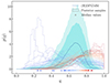 |
Fig. B.1. Marginalised FIGARO reconstruction of the observed mass-ratio distribution (blue solid line – median – and shaded regions – 68% and 90% credible regions) along with individual event posterior samples (histograms) coloured according to their median values (triangular markers). |
We can define consistency with q = 1 as p(q > 0.95), finding that 41 events out of 62 have a probability greater than 5% of having q > 0.95. At the same time, however, only 16 events out of 62 have a probability of greater than 10%, and none of them have a probability of greater than 20%9. Moreover, the largest median value among all the posterior distributions is q = 0.86, from GW150914. With these things in mind, we see that the inferred observed distribution in Fig. B.1 is consistent with the observations. In particular, the median distribution is consistent with the median values for individual posteriors, with the credible regions accounting for the possible combined fluctuations of the individual posteriors, q ∼ 0.98. These heuristic arguments suggest that our reconstruction is in agreement with the available observations.
The lack of support for symmetric binaries is then further enhanced by the inclusion of selection effects, which favour asymmetric binaries, and the conversion of the astrophysical distribution into the differential merger rate, leading to the distribution we report in the main text of this paper.
Appendix C: Validation with simulated data
In this section, we show that (H)DPGMM and FIGARO successfully reconstruct a probability density modelled after the findings of Abbott et al. (2023c) in M1 and q with just the small number of events presently available. This is to validate the results presented in this paper and to strengthen the claim that the features we find are due to the actual astrophysical population and not to some artefacts of the model, particularly for what concerns the shape of the mass-ratio distribution.
We generated the mock catalogue of GW events using a rejection sampling approach as follows:
-
i)
We drew a set of mock binary parameters from the simulated astrophysical distribution for M1, q, and z. In particular, the primary mass follows a tapered power-law distribution with a Gaussian peak,
and the mass ratio is distributed according to a power law,
The redshift distribution is taken to be Gaussian, centred around μz,
This choice for p(z) is dictated by the need to have a model with no significant support in the low-mass, high-redshift region of the parameter space, which is censored by the selection function. A significant support in this region would lead to a bias, as explained in Appendix D. We specify the parameters of these distributions in Table C.1.
-
ii)
For each simulated BBH, we evaluated the detection probability pdet(M1, q, z) using the selection function by Lorenzo-Medina & Dent (in prep.). For each sample, we then uniformly drew a number h between 0 and 1: we labelled all the binaries with h < pdet as ‘detected’.
-
iii)
For every detected binary, we generated a set of 2000 posterior samples under the simplifying assumption that the posterior distribution is an uncorrelated multivariate Gaussian distribution in log M1,
 and log z. We made sure that such mock posteriors pass the pp-plot test.

Parameters of the simulated astrophysical distribution presented in Appendix C.
Our mock catalogue contains 64 events, a number comparable with GWTC-3. Figure C.1 shows the posterior distribution recovered with FIGARO after correcting for selection effects, along with the simulated distribution.
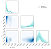 |
Fig. C.1. FIGARO reconstruction (blue) of the M1, q and z simulated distribution (red). The diagonal panels show the marginal distributions for M1, q, and z (top to bottom) respectively and the panels below diagonal show the median distribution marginalised over the third variable. |
The non-parametric reconstruction is able to capture all the features that are present in the simulated distribution within the 90% credible region. In particular, the power-law behaviour of the mass-ratio distribution is correctly recovered even with as few as 64 events, supporting our finding that the astrophysical mass-ratio distribution has little to no support at q = 1.
Appendix D: Censored data
Selection effects act as a filter for the astrophysical distribution, modifying the probability of observing a specific binary merger. These effects are due to several factors: among others, we mention the detector noise, the efficiency of the search pipelines, and the validity range of waveform models.
In the framework we apply in this paper, we can correct for selection effects following Eq. (5), under the assumption that we properly sampled all the regions of the parameter space. This assumption does not hold, however, in a case where the astrophysical distribution has support in a region where the detection probability is negligible10 or exactly zero, such as in a region of the parameter space not covered by any waveform model. The selection function would in this case censor a portion of the data.
An astrophysical distribution that extends its support in a censored region would not therefore be reconstructed properly by a non-parametric method: the observed distribution would be cut off by the selection function, biasing the subsequent inference of the astrophysical distribution.
In Fig. D.1 we show the behaviour of an observed distribution obtained filtering an astrophysical distribution that has support in a censored region of the selection function used throughout this paper (Lorenzo-Medina & Dent in prep.). The simulated underlying distribution is the same as in Appendix C, with the exception of p(z):

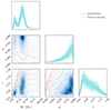 |
Fig. D.1. Observed distribution for the simulated catalogue reconstructed with FIGARO (blue line) along with the iso-probability levels of the selection function (red). The diagonal panels show the marginal distributions for M1, q and z (top to bottom) respectively and the panels below diagonal show the median distribution marginalised over the third variable. |
In the low-mass, high-redshift region, the median two-dimensional M1 − z distribution follows the iso-probability curves of the selection function, suggesting that a portion of the data has been censored. Conversely, this behaviour is not seen for the credible regions of the observed distribution reconstructed with GWTC-3 (reported in Fig. D.2) suggesting, although heuristically, that we are not dealing with censored data.
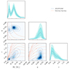 |
Fig. D.2. Observed distribution for GWTC-3 reconstructed with FIGARO (blue line) along with the iso-probability levels of the selection function (orange). The diagonal panels show the marginal distributions for M1, q, and z (top to bottom) respectively and the panels below diagonal show the median distribution marginalised over the third variable. |
All Tables
Parameters of the simulated astrophysical distribution presented in Appendix C.
All Figures
|
Fig. 1. Primary mass differential merger rate density reconstructed with FIGARO along with the POWERLAW+PEAK model from Abbott et al. (2023c). The shaded areas correspond to 68 and 90% credible regions for (H)DPGMM (blue) and POWERLAW+PEAK (orange). |
| In the text | |
|
Fig. 2. M1, q and z differential merger rate density reconstructed with FIGARO as in Eq. (6). The diagonal panels show the marginal distributions for M1, q and z (top to bottom), respectively, and the panels below diagonal show the median distribution marginalised over the third variable. |
| In the text | |
|
Fig. 3. Mass ratio evolution with redshift: joy plot (a) and tomography (b). Both panels report the median distribution only: an animated version of this plot including the 68% credible regions is available online along with plots showing individual slices. This distribution, set aside an excess at low redshifts (z ≲ 0.2), is consistent throughout the whole redshift spectrum in having support at around 0.7, with negligible support for q = 1. |
| In the text | |
|
Fig. 4. Primary mass evolution with redshift: joy plot (a) and tomography (b). Both panels report the median distribution only: an animated version of this plot including the 68% credible regions is available online along with plots showing individual slices. The mass distribution drastically changes with redshift, suggesting the presence of two distinct populations of BHs. |
| In the text | |
|
Fig. 5. Primary mass conditional differential merger rate density for the local Universe (z ≤ 0.2) compared with a power-law distribution (index α from Abbott et al. 2023c). Shaded areas correspond to 68% credible regions. |
| In the text | |
|
Fig. 6. Evolution of the peak of the pileup feature of the mass distribution with redshift. The peak is defined as the maximum of the distribution for M1 > 25 M⊙. The shaded areas correspond to the 68 and 90% credible regions. |
| In the text | |
|
Fig. 7. Primary mass conditional differential merger rate density for z = 0.8. The shaded area correspond to the 68% credible region. The peak at M1 ∼ 90 M⊙ marks the presence of GW190521. |
| In the text | |
|
Fig. B.1. Marginalised FIGARO reconstruction of the observed mass-ratio distribution (blue solid line – median – and shaded regions – 68% and 90% credible regions) along with individual event posterior samples (histograms) coloured according to their median values (triangular markers). |
| In the text | |
|
Fig. C.1. FIGARO reconstruction (blue) of the M1, q and z simulated distribution (red). The diagonal panels show the marginal distributions for M1, q, and z (top to bottom) respectively and the panels below diagonal show the median distribution marginalised over the third variable. |
| In the text | |
|
Fig. D.1. Observed distribution for the simulated catalogue reconstructed with FIGARO (blue line) along with the iso-probability levels of the selection function (red). The diagonal panels show the marginal distributions for M1, q and z (top to bottom) respectively and the panels below diagonal show the median distribution marginalised over the third variable. |
| In the text | |
|
Fig. D.2. Observed distribution for GWTC-3 reconstructed with FIGARO (blue line) along with the iso-probability levels of the selection function (orange). The diagonal panels show the marginal distributions for M1, q, and z (top to bottom) respectively and the panels below diagonal show the median distribution marginalised over the third variable. |
| In the text | |
Current usage metrics show cumulative count of Article Views (full-text article views including HTML views, PDF and ePub downloads, according to the available data) and Abstracts Views on Vision4Press platform.
Data correspond to usage on the plateform after 2015. The current usage metrics is available 48-96 hours after online publication and is updated daily on week days.
Initial download of the metrics may take a while.