| Issue |
A&A
Volume 681, January 2024
|
|
|---|---|---|
| Article Number | A100 | |
| Number of page(s) | 12 | |
| Section | Extragalactic astronomy | |
| DOI | https://doi.org/10.1051/0004-6361/202347669 | |
| Published online | 22 January 2024 | |
MUSE observations of the giant low surface brightness galaxy Malin 1: Numerous HII regions, star formation rate, metallicity, and dust attenuation⋆
1
National Centre for Nuclear Research, Pasteura 7, 02-093 Warsaw, Poland
e-mail: This email address is being protected from spambots. You need JavaScript enabled to view it.
2
Leibniz-Institut für Astrophysik Potsdam (AIP), An der Sternwarte 16, 14482 Potsdam, Germany
3
Aix-Marseille Univ., CNRS, CNES, LAM, Marseille, France
4
Canada-France-Hawaii Telescope, 65-1238 Mamalahoa Highway, Kamuela, HI 96743, USA
5
Instituto de Astrofísica, Pontificia Universidad Católica de Chile, Avenida Vicuña Mackenna 4860, 7820436 Macul, Santiago, Chile
6
Instituto de Estudios Astrofísicos, Facultad de Ingeniería y Ciencias, Universidad Diego Portales, Av. Ejército Libertador 441, Santiago, Chile
Received:
7
August
2023
Accepted:
17
October
2023
Abstract
Context. Giant low surface brightness (GLSB) galaxies are an extreme class of objects with very faint and extended gas-rich disks. Malin 1 is the largest GLSB galaxy known to date and one of the largest individual spiral galaxies observed so far, but the properties and formation mechanisms of its giant disk are still poorly understood.
Aims. We used VLT/MUSE IFU spectroscopic observations of Malin 1 to measure the star formation rate (SFR), dust attenuation, and gas metallicity within this intriguing galaxy.
Methods. We performed a penalized pixel fitting modeling to extract emission line fluxes such as Hα, Hβ, [N II]6583 and [O III]5007 along the central region as well as from the extended disk of Malin 1.
Results. Our observations reveal for the first time strong Hα emission distributed across numerous regions throughout the extended disk of Malin 1. The emission extends to radial distances of ∼100 kpc, which indicates recent star formation activity. We made an estimate of the dust attenuation in the disk of Malin 1 using the Balmer decrement and found that Malin 1 has a mean Hα attenuation of 0.36 mag. We observe a steep decline in the radial distribution of the SFR surface density (ΣSFR) within the inner 20 kpc, followed by a shallow decline in the extended disk. We estimated the gas phase metallicity in Malin 1. We also found for the first time that the metallicity shows a steep gradient from solar metallicity to subsolar values in the inner 20 kpc of the galaxy, followed by a flattening of the metallicity in the extended disk with a relatively high value of ∼0.6 Z⊙. We found that the normalized abundance gradient of the inner disk of Malin 1 is similar to the values found in normal galaxies. However, the normalized gradient observed in the outer disk can be considered extreme when compared to other disk galaxies. A comparison of the SFR surface density and gas surface density shows that unlike normal disk galaxies or other low surface brightness galaxies, the outer disk of Malin 1 exhibits a relatively low star formation efficiency based on atomic gas-mass estimates, which may be mildly exacerbated by the vanishing upper molecular gas-mass limits found by recent CO studies.
Conclusions. With the detection of emission lines in a large part of the extended disk of Malin 1, this work sheds light on the star formation processes in this unique galaxy, highlighting its extended star-forming disk, dust attenuation, almost flat metallicity distribution in the outer disk, and exceptionally low star formation efficiency. Together with previous results, our findings contribute to a more detailed understanding of the formation of the giant disk of Malin 1, and they also constrain possible proposed scenarios of the nature of GLSB galaxies in general.
Key words: galaxies: individual: Malin 1 / galaxies: star formation / galaxies: abundances / galaxies: ISM
Emission line maps are available at the CDS via anonymous ftp to cdsarc.cds.unistra.fr (130.79.128.5) or via https://cdsarc.cds.unistra.fr/viz-bin/cat/J/A+A/681/A100
© The Authors 2024
 Open Access article, published by EDP Sciences, under the terms of the Creative Commons Attribution License (https://creativecommons.org/licenses/by/4.0), which permits unrestricted use, distribution, and reproduction in any medium, provided the original work is properly cited.
This article is published in open access under the Subscribe to Open model. This email address is being protected from spambots. You need JavaScript enabled to view it. to support open access publication.
1. Introduction
Low surface brightness galaxies (LSBs) form a diverse class of galaxies that exhibit significantly lower brightness per unit area than normal high surface brightness galaxies, and their surface brightness is certainly lower than the dark night sky. In the past decade, LSBs have obtained much attention because their characteristics are extreme and because they might have implications for our understanding of galaxy formation scenarios. LSBs are commonly defined as galaxies with an average r-band surface brightness ( ) below the typical level of the night sky (
 mag arcsec−2; Martin et al. 2019; Junais et al. 2023). LSBs have a distinct subpopulation that is known as giant LSB galaxies (GLSBs). These have a massive faint extended disk and are rich in gas content (Bothun et al. 1987; Sprayberry et al. 1995; Matthews et al. 2001).
Malin 1 is the archetype of GLSB galaxies and has captivated the attention of astronomers since its accidental discovery nearly four decades ago (Bothun et al. 1987). Malin 1 has a radial extent of ∼120 kpc at least (Moore & Parker 2006) and an extrapolated central disk central surface brightness of μ0, V ≈ 25.5 mag arcsec−2 (Impey & Bothun 1997). Despite its faint surface brightness disk, Malin 1 has a total absolute magnitude of MV ≈ −22.9 mag (Pickering et al. 1997) and an HI mass of approximately 5 × 10¹⁰ M⊙ (Pickering et al. 1997; Matthews et al. 2001). It is currently considered the largest known spiral galaxy. Malin 1 is situated in a relatively low-density environment in the large-scale structure with close proximity to a filament, offering the stability and richness of its huge gaseous disk (Junais 2021).
The Hubble Space Telescope (HST) i-band image analysis by Barth (2007) identified a normal barred inner spiral disk embedded within an extensive diffuse LSB disk in Malin 1. This is similar to galaxies with extended ultraviolet (XUV) disks that are found in approximately 30% of nearby galaxies (Thilker et al. 2007). The extension and scope of the enormous spiral arms of Malin 1 were shown by Galaz et al. (2015). Later, Boissier et al. (2016) performed an analysis of the radial stellar profiles and suggested that the angular momentum of the extended disk of Malin 1 is about 20 times higher than that of the Milky Way. Therefore, Malin 1 represents an extreme case in the class of GLSBs. The nature and origin of these GLSBs are still poorly understood, although more GLSBs that were less extreme, however, were discovered over the years (Hagen et al. 2016; Saburova et al. 2021). In recent work, Saburova et al. (2023) suggested that GLSBs are not rare objects, as was thought previously. Based on their predicted GLSB volume density, ∼13 000 GLSBs could exist within the local Universe at z < 0.1. It is expected that with the deep Legacy Survey of Space and Time (LSST; Ivezić et al. 2019), we will soon be able to uncover even more of these faint giant galaxies.
Despite its significance, Malin 1 has been subject to only a few spectroscopic studies. Previous efforts have primarily relied on velocity maps with low spatial resolution obtained from HI data (Lelli et al. 2010), along with optical spectra of the central region from SDSS observations (Subramanian et al. 2016). Later, Junais et al. (2020) performed a spectroscopic analysis of Malin 1 using long-slit data obtained from the IMACS/Magellan spectrograph, focusing mostly on the central region (< 10 kpc) of Malin 1, along with only one small region detected in the extended disk (at ∼25 kpc radius). The lack of an in-depth spectroscopic analysis of Malin 1, especially of its large extended disk, hinders a comprehensive understanding of its properties and formation.
In this work, we present a spectroscopic study of Malin 1 based on data obtained with the MUSE Integral Field Unit (IFU), aiming to shed light on the nature and formation of this extraordinary GLSB galaxy. Based on these data, we perform a detailed analysis of the star formation rate (SFR) and dust attenuation of Malin 1, and we analyze the gas-phase metallicity of its extended disk. Throughout this work, we adopt a flat ΛCDM cosmology with H0 = 70 km s−1 Mpc−1, ΩM = 0.27, and ΩΛ = 0.73, which corresponds to a projected angular scale of 1.56 kpc arcsec−1 and to a luminosity distance of 377 Mpc.
The paper is structured as follows: Sect. 2 provides an overview of the data and observations, including the MUSE IFU data acquisition and reduction process. Section 3 focuses on the analysis and results. Sections 4 and 5 present the discussion and conclusions, respectively.
2. Observation and data analysis
Malin 1 was observed with the VLT/MUSE integral field spectrograph (Bacon et al. 2010) on 18 April 2021 under program ID 105.20GH.001 (PI: Gaspar Galaz). The galaxy covers more that 2′×2′ on the sky, but the field of view of MUSE is 1′×1′, with a sampling scale of 0.2″ pixel−1. Out of the four planned MUSE pointings, only the northern quadrant of Malin 1 was observed (see Fig. 1). However, the center of the galaxy was well covered. Observations were conducted at an airmass of ∼1.3 and an external seeing of ∼1.2″. The observations were carried out with four exposures, resulting in a total exposure time of 4640 s. The spectral resolving power ranges from R ≃ 1770 at 4800 Å to R ≃ 3590 at 9300 Å. The observations used the ground-layer adaptive optics (AO) system (Ströbele et al. 2012) so that the full width at half maximum (FWHM) in the MUSE instrument at 7000 Å was estimated to be  from the telemetry of the AO system (Fusco et al. 2020).
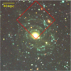 |
Fig. 1. Color-composite image of Malin 1 from the Canada-France-Hawaii Telescope (CFHT) Megacam NGVS survey u-, g-, and i-band images (Ferrarese et al. 2012). The image spans a width of ∼2.6′×2.6′. The red box shows the MUSE field of observation (1′×1′). |
2.1. Data reduction
We reduced the data with the MUSE pipeline (v2.8; Weilbacher et al. 2020) called from the ESO Recipe Execution Tool (EsoRex) tool. We largely used standard processing, including the creation of master bias, flat field, and trace tables, and we derived wavelength solutions separately for each CCD, with an overall twilight-sky correction for the whole field, all with default parameters. We also used standard bad pixel and geometry tables as well as a line-spread function that was automatically associated with the data by the ESO archive. All master calibrations were then applied to the raw on-sky data (standard stars, science exposures, and offset sky fields). While the standard star (HD 49798) observed at the beginning of the night was usable for the flux calibration, we used two other standard star exposures to derive the telluric correction (LTT 3218 from 14 April 2021 and EG 274 taken on 14 April 2021). These provide a good match in the integrated water vapor levels (recorded in the IWV keywords in the raw data headers) and hence correct the telluric A and B bands better. The science data were corrected for the sky background using internal sky instead of the offset sky fields because the spiral arms of Malin 1 fill only a portion of the MUSE field. The data were further corrected for distortions using the provided astrometric calibration and were shifted to a barycentric velocity frame. All four science exposures were aligned using a star from the Gaia EDR3 catalog (Lindegren et al. 2021) and were combined to form a single data cube with wavelength coverage 4595−9350 Å. The final spatial FWHM measured in the reconstructed R band is  .
.
2.2. Emission line fitting
To disentangle the ionized gas emission lines from the stellar continuum and measure their fluxes corrected for hydrogen absorption, we used the penalized pixel-fitting (pPXF) tool throughout (v8.2.4; Cappellari 2017). To maximize the detection in different regions of Malin 1, we employed several approaches for the emission line fitting. This is described in the following subsections.
2.2.1. Central region
In the central region of Malin 1 (21″ × 21″), where the stellar continuum is strong, we performed a spectral binning using the Voronoi algorithm of Cappellari & Copin (2003) to target a final signal-to-noise ratio (S/N) ≈20. We included only the spatial pixels (spaxels) in which the median continuum S/N in the wavelength range 5600−6500 Å was 1 at least. Then, the pPXF was set up on the binned spectra of the central region to simultaneously fit the continuum, using the GALEV SSPs (Kotulla et al. 2009) constructed with the Munari stellar library (Munari et al. 2005) as templates and the known strong emission lines between Hγ and Pa14 (corresponding to the restframe λ-range at the redshift of Malin 1) modeled as Gaussian peaks. To reduce the effects of flux calibration inaccuracies, we employed a multiplicative polynomial of order 7. The same setup was employed and discussed in more detail by Weilbacher et al. (2018) and Micheva et al. (2022). Lines falling into masked spectral regions1 at the redshift of Malin 1 were excluded. As initial guesses for the kinematics, we used z = 0.08 for the velocity and σ = 75 km s−1, for both stars and gas. We verified this setup against the default setup of pPXF using the E-MILES SSP templates (Vazdekis et al. 2016). Because we found no significant differences, we use the results from the GALEV+Munari setup in the following part of this work because they produce fits with fewer residuals or artifacts. All emission line flux measurements were then projected back into the 2D plane to form a map (see Fig. 2).
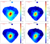 |
Fig. 2. Emission line flux maps of the central region of Malin 1 (21″ × 21″) obtained from the pPXF fitting. The Hα and the Hβ lines are shown in the top panels, and the [N II]6583 and the [O III]5007 lines are shown in the bottom panels. The color bar indicates the flux corresponding to each line. |
2.2.2. Extended disk regions
To extract emission line fluxes in the whole MUSE field, including in the extended disk of Malin 1, we first defined H II regions using the dendrogram algorithm (using the Python package astrodendro2), which tracks isophotal contours around peaks in images. It creates a tree-like structure that allows us to relate leaves (contours within which only a single peak is located) to branches (contours containing several leaves). We ignored the hierarchical nature of the data structure and just used the leaves, which represent the largest contour around a peak that has not merged with neighboring peaks, such as the H II regions. As input, we used an Hα image created by fitting a Gaussian function to the expected redshifted emission line in each spaxel of the cube. We filtered this image with a 2D Gaussian function with  FWHM to enhance real features. Peaks are detected above a limit of 1.5 × 10⁻¹⁹ erg s−1 cm−2, with a minimum number of 9 pixels above the limit. We did not impose a limit on the height of the peaks. We detected 62 peaks in the cube and extracted spectra and data variance by averaging them over the spaxels of the corresponding leaves (H II regions) defined by astrodendro. They were saved as row-stacked spectra and subsequently input to pPXF, as discussed in Sect. 2.2.1, to extract emission line fluxes. Only the line fluxes with an S/N > 2.5 were used in this analysis. We found that this approach of fitting the integrated spectrum of a region significantly increases the S/N compared to a pixel-level fitting and hence increases the number of regions (by a factor of about 8) with faint emission line measurements (Hβ, [N II]6583 and [O III]5007). Figure 3 shows the emission line maps of all the identified regions. Several Hα regions in the disk of Malin 1 are clearly detected, most of which extend up to ∼80 kpc from the center of the galaxy. One region is detected at a radius of about 100 kpc (ID 62 in Fig. 3).
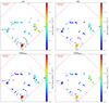 |
Fig. 3. Emission line flux maps of Malin 1 obtained from the pPXF fitting of the H II regions. The Hα, and the Hβ lines are shown in the top panels, and the [N II]6583 and the [O III]5007 lines are shown in the bottom panels. The ID of each region, as discussed in Sect. 2.2.2, is labeled in black in the top left panel. The regions with ID 27 and 49 are excluded from the maps as they do not have an S/N > 2.5 in any of the emission lines. The color bar indicates the flux corresponding to each emission line. The flux value of each region is given as the average flux per pixel within that region obtained from the fitting of its row-stacked spectrum. |
2.2.3. Hα radial average
In addition to the fitting of the central region and the selected H II regions in the extended disk, we also performed an integrated spectral fitting for several radial bins of Malin 1. This was done to estimate the Hα radial average fluxes within the galaxy. For this purpose, we placed 14 concentric rings on the MUSE cube, starting from the center of Malin 1 to a radial distance of ∼100 kpc. each ring had a width of 5″ (7.8 kpc). Then we followed a similar approach as discussed in Sect. 2.2.2 by stacking all the spaxels within a ring to obtain its corresponding integrated spectrum. However, as each radial bin spans several kiloparsec, resulting in azimuthal variations in the line-of-sight velocity, we needed to correct for these velocity variations in the spaxels of a ring to generate integrated spectra with a high S/N3.
To correct for the velocity variations, we extracted moment maps and masks over the whole MUSE field of view using the Python software CAMEL4 (see Epinat et al. 2012) on the group of emission lines Hα, [S II]λλ6716,6731, and [N II]λλ6548,6583. In order to avoid local velocity variations and to increase the sensitivity at the edge of emitting regions and thus increase the spatial extent, the MUSE datacube was first smoothed using a 2-pixel FWHM Gaussian kernel. Only the spaxels within the wavelength range corresponding to the redshift range 0.0714 < z < 0.0934 were considered around each line within the MUSE cube in order to have some continuum, but with a reasonable weight in the fit. CAMEL then fit all lines and the continuum simultaneously for each spaxel of the MUSE cube, taking advantage of the variance cube produced during data reduction. Lines were modeled as Gaussian functions, using a common velocity, but with a width that varied from one species to the next because the two lines in a doublet were expected to have the same origin and were close enough in wavelength to avoid line-spread function variations. The continuum was adjusted with a third-degree polynomial function. Flux maps were generated for all fitted emission lines, together with associated error maps, as well as S/N maps, velocity dispersion fields, and the velocity field. We further computed a spatial mask in order to exclude regions in which no signal was coherent with the large-scale velocity pattern. We removed all pixels with an S/N in the Hα line below 2.5 and with velocities that were incompatible with Malin 1. We further removed spurious isolated groups of pixels smaller than 1″ in diameter, which is smaller than the seeing FWHM of the observations.
After these maps were generated, the inferred velocity was used to compute the wavelengths at which the spectrum was actually sampled in the restframe corresponding to the systemic velocity of Malin 1 for each spaxel of the original unsmoothed datacube. The spectrum at each spaxel was then resampled on a single spectral grid for all spaxels by performing a linear interpolation to apply the velocity correction. Finally, for each ring, we summed all spaxels at the restframe of Malin 1 that lay within both the ring and mask to produce the corresponding integrated spectrum. We performed a pPXF fit on these spectra as discussed in Sect. 2.2.1 to obtain the radial average Hα fluxes in each ring (the average Hα flux in each ring was obtained by dividing the total flux by the unmasked ring area). We only included the Hα fluxes with an S/N > 2.5 in this work (11 among the 14 rings).
From here on, we corrected all the observed emission line fluxes from Sect. 2.2 for foreground Galactic extinction using the Schlegel et al. (1998) dust maps and the Cardelli et al. (1989) Milky Way dust extinction law.
3. Results
3.1. Balmer decrement and dust attenuation
The Balmer ratio (Hα/Hβ flux ratio) is commonly used as a diagnostic tool for dust attenuation in galaxies (e.g., Domínguez et al. 2013; Boselli et al. 2015). The intrinsic Balmer ratio, (Hα/Hβ)int, remains roughly constant for typical gas conditions in galaxies. For case B recombination5, (Hα/Hβ)int = 2.86 (Osterbrock 1989). Therefore, we can obtain the attenuation at a wavelength, Aλ, by comparing the observed Balmer ratio with the theoretical value following Eq. (6) of Yuan et al. (2018),
![Mathematical equation: $$ \begin{aligned} A_{\lambda } = -2.5\frac{k(\lambda )}{k(\mathrm{H}\alpha ) - k(\mathrm{H}\beta )} \log \left[\frac{(\mathrm{H}\alpha /\mathrm{H}\beta )_{\rm obs}}{2.86}\right], \end{aligned} $$](/articles/aa/full_html/2024/01/aa47669-23/aa47669-23-eq6.gif) (1)
(1)
where k(λ) is the value of the attenuation curve at a wavelength λ, and (Hα/Hβ)obs is the observed Balmer ratio. Assuming a Calzetti et al. (2000) dust attenuation law with RV = 4.05, we obtain k(Hα) = 3.33; k(Hβ) = 4.60; k([NII]6583) = 3.31 and k([OIII]5007) = 4.46. We can then obtain the attenuation for all the emission lines presented in this work using Eq. (1).
Figure 4 shows our observed Balmer ratio and Hα attenuation. The central region of Malin 1 (< 10 kpc) has a wide range of Balmer ratios up to 5, with a mean value of about 3.26. This corresponds to an Hα attenuation (AHα) up to 1 mag, with a mean attenuation of ∼0.3 mag. Similar to the central region, the mean Balmer ratio is 3.25 and AHα of 0.43 mag in the extended disk. We thus conclude that the dust attenuation in the central and extended disk regions of Malin 1 is non-negligible with a mean AHα = 0.36 mag.
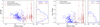 |
Fig. 4. Radial variation of the Balmer ratio (left panel) and Hα attenuation (right panel). The blue circles and the brown hexagons show the central regions and the extended disk regions, respectively, obtained from the pPXF fit discussed in Sect. 2.2. The horizontal dashed red line marks the intrinsic Balmer ratio of 2.86 for case B recombination. To all regions in which the Balmer ratio was below this value, we assigned zero attenuation. The histograms next to each panel give the overall distribution of each quantity (the solid blue line and the dashed brown line show the central region and extended disk, respectively). Their mean values are indicated at the top of each panel. |
3.2. Star formation rate surface density
We used our Hα emission line flux measurements to estimate the radial variation of the SFR surface density (ΣSFR) in Malin 1. The measured Hα fluxes were converted into the SFR following Boissier (2013) and a Kroupa (2001) initial mass function (IMF) using
 (2)
(2)
where LHα is the Hα luminosity corresponding to the observed Hα flux. The Hα fluxes before the estimation of the SFR were corrected for dust attenuation using the attenuation measurements discussed in Sect. 3.1. The SFR values were converted into ΣSFR by dividing by the area in which the Hα flux was measured.
Figure 5 shows the ΣSFR as a function of galactocentric radius. In this plot, we also show the average ΣSFR estimated from the Hα radial average measurements discussed in Sect. 2.2.3. While the local measurements are indicative of individual star-forming regions, radial averages are meaningful for understanding the galaxy evolution over orbital timescales to compare to 1D models depending on the galactocentric radius, or to the gas distribution over large scales. We find a steep gradient in ΣSFR within the central 10 kpc of the galaxy. This is consistent with the long-slit observations of Malin 1 from Junais et al. (2020). Beyond the central regions, the ΣSFR is mostly flat at about ΣSFR ∼ 10−4 M⊙ yr−1 kpc−2 for the extended disk regions, but based on the radial average measurements, there is a shallow decline to about ∼10−6 M⊙ yr−1 kpc−2 until 100 kpc. However, a clear spike appears in ΣSFR around 50 to 60 kpc radius in the Hα selected regions and in the radial average estimates. This corresponds to the extended bright star-forming regions that were found at this radius, as is clearly shown in the Hα map from Fig. 3. The ΣSFR of these individual star-forming regions is higher in general than the average radial values. For comparison, we estimated a similar radial average of ΣSFR using the Ultra Violet Imaging Telescope (UVIT) far-UV (FUV) image of Malin 1 from Saha et al. (2021) in the same field as our Hα observations, and we obtained a similar peak6. The attenuation at the FUV wavelength was obtained by adopting a Calzetti et al. (2000) attenuation and a gas-to-stellar reddening factor of 0.44, as discussed in Sect. 4. Figure 6 clearly shows that most of the bright Hα regions coincide well with the UV blobs. These UV blobs were not resolved in the previous GALEX images of Malin 1 from Boissier et al. (2016). The improved angular resolution of the UVIT images (∼1.6″; Saha et al. 2021) is three times better than that of GALEX. Many Hα-bright regions we observe can be identified as resolved individual regions in the UVIT image. Similarly, the ΣSFR values based on the UV data are well consistent with the estimates from the Hα measurements within their uncertainties (see Fig. 5), although many UV radial points only provide an upper limit in ΣSFR, while the Hα determination is well constrained by our spectral stacking technique discussed in Sect. 2.2.3. We also performed a UV radial average measurement of ΣSFR for the full galaxy (instead of only the one quarter for which we have MUSE observations) and found that they are very similar to our initial estimates. The difference is smaller than 0.1 dex.
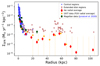 |
Fig. 5. SFR surface density of Malin 1 as a function of galactocentric radius. The blue circles and brown hexagons show the central regions and the extended disk regions, respectively, obtained from the pPXF fit discussed in Sect. 2.2. The red diamonds are the Hα radial average measured in concentric rings with a width of 5″ from the center. The orange stars show the radial averages measured in the same field in the UVIT FUV image of Malin 1 from Saha et al. (2021), as shown in Fig. 6. For illustration purposes, the UV data points are horizontally shifted by 2 kpc. The green squares show the data points from Junais et al. (2020), based on the IMACS-Magellan Hα long-slit spectra of Malin 1. |
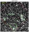 |
Fig. 6. FUV image of Malin 1 from Saha et al. (2021) of the same field as our MUSE observations (shown as the red box). The green contours mark the Hα-detected regions, as discussed in Sect. 2.2.2. |
3.3. Metallicity
We estimated the radial variation in metallicity in Malin 1 using the observed emission lines. We used the N2 and the O3N2 metallicity calibrators from Marino et al. (2013), given as
 (3)
(3)
 (4)
(4)
where the flux ratios are encoded as N2 = log([NII]6583/Hα) and O3N2 = log([OIII]5007/Hβ)−log([NII]6583/Hα).
Figure 7 shows the radial metallicity distribution of Malin 1. The metallicity estimate based on the N2 calibrator indicates that the metallicity in the central region of the galaxy (within a few kiloparsec) is nearly solar, whereas the metallicity in the inner disk out to 20 kpc has a steep gradient that reaches subsolar values (∼0.65 Z⊙). However, for the outer disk beyond 20 kpc, the metallicity flattens (∼0.6 Z⊙), consistent with no or a shallow slope, compared to the central regions. This behavior is also found in XUV disk galaxies such as M 83 (Bresolin et al. 2009; Bresolin 2017) and NGC 1512 (López-Sánchez et al. 2015). The calibrators of N2 and the O3N2 both show a similar trend, although the metallicity estimated from O3N2 is lower in general than the N2 estimates by about 0.07 dex on average. This offset among different strong-line calibrations is often found in the literature as a result of differences in the excitation parameter and ionization states of the various lines that were used (e.g., Kewley & Ellison 2008; Micheva et al. 2022). For instance, Kewley & Ellison (2008) showed that offsets among different calibrations can reach 0.6 dex in metallicity, and with a large scatter. This is consistent with the offset of 0.07 dex we obtained between our N2 and O3N2 estimates. Other commonly used metallicity calibrators in the literature, such as R23 or N2O2, cannot be estimated using our data because the emission lines required for those calibrators are not within the MUSE spectral coverage.
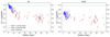 |
Fig. 7. Radial variation of the metallicity of Malin 1. Left: metallicity using the N2 calibrator of Marino et al. (2013). Right: metallicity using the O3N2 calibrator of Marino et al. (2013). The blue circles and brown hexagons show the central regions and extended disk regions, respectively, as discussed in Sect. 2.2. The horizontal dotted green line marks the solar metallicity. The uncertainty of the N2 and O3N2 calibrations from Marino et al. (2013) is 0.16 dex and 0.18 dex, respectively. |
Table A.1 provides the measured quantities of all the Hα-selected regions in the extended disk of Malin 1 we discuss in this section. Based on the Hα fluxes from Table A.1, it is interesting to note that we observe Hα luminosities (LHα) in the range of 1038 − 1040 erg s−1 (with a median LHα of 1038.7 erg s−1), similar to the range found for H II regions of LSB galaxies by Schombert et al. (2013). However, due to the limited resolution that prevents us from resolving individual H II regions at the distance of Malin 1, it is hard to make a direct comparison.
4. Discussion
4.1. Dust attenuation in Malin 1
LSBs are generally considered to be dust poor (Hinz et al. 2007; Rahman et al. 2007; Liang et al. 2010). However, these results are based on either very small samples or on shallow data. Recently, Junais et al. (2023) performed a large statistical analysis of the dust content in 1003 LSBs using deep data and found that although a fraction of LSBs is dust poor, ∼4% contain high dust attenuation. However, they observed that these LSBs with high attenuation are also similar to the GLSBs in terms of their average stellar mass surface density and surface brightness. This may indicate a higher dust attenuation in GLSBs.
Our dust attenuation measurements of Malin 1 show that this is indeed the case. We observe a non-negligible amount of dust attenuation in the central region as well as in the extended disk of Malin 1. Junais et al. (2023) calibrated the variation of attenuation as a function of the stellar mass surface density. Their Eq. (3) predicts that a Malin 1-like galaxy with an average stellar mass surface density of 107.9 M⊙ kpc−2 should have an attenuation AV of about 0.33 mag. The mean Hα attenuation we obtained for Malin 1 corresponds to nearly 0.36 mag. This is consistent with the scaling relation predictions by Junais et al. (2023).
The extended disk of Malin 1 is undetected in Spitzer (Hinz et al. 2007), Herschel (Boissier et al. 2016), and WISE7 imaging. For instance, Hinz et al. (2007) found that Malin 1 has a 1σ upper flux limit of 10 mJy in the Spitzer MIPS 160 μm observations. Our observed measurements of attenuation in the disk of Malin 1 challenge these nondetections. However, by construction, our relatively high attenuation8 is found in star-forming regions that cover only a small fraction of the extended disk (see Fig. 3). The relation between the gas and the stellar attenuation has been discussed extensively in the literature. Calzetti (1997) proposed a factor of 0.44 between the gas and the stellar reddening as E(B − V)star = 0.44 E(B − V)gas. Lin & Kong (2020) investigated this relation for a large sample of galaxies with a wide range of physical properties and found that this relation varies with several galaxy properties. The low covering fraction of star-forming regions in Malin 1 could be related to the low attenuation suggested by optical broadband studies. This calls for deeper observations of Malin 1 at mid-IR (MIR) and far-IR (FIR) wavelengths. Moreover, exploring the geometric distribution of the dust and stars could also provide insights into the measured high attenuation and current nondetections at IR wavelengths (e.g., Hamed et al. 2023).
An alternative explanation of this discrepancy might be that the conditions in the star-forming regions of Malin 1 are characterized by partial self-absorption of Balmer photons, which is synonymous with mildly optically thick conditions. These conditions would increase the expected Balmer ratio and consequently decrease the expected dust attenuation, making it more consistent with previous IR measurements.
4.2. Correlation of radial gas metallicity and stellar profile
Figure 8 (top panel) shows the radial variation in the gas-phase metallicity using the N2 calibrator in Malin 1. For the first time, we observe a relatively steep decline from the solar metallicity in the inner region of Malin 1, followed by a flattening of the metallicity around 0.6 Z⊙ beyond the 20 kpc radius. The radius at which this flattening occurs also coincides with the i-band optical break radius of Malin 1 (19.6 kpc) found by Junais et al. (2020). This latter break radius corresponds to the transition from the inner to the outer disk, based on a broken exponential disk profile (Erwin et al. 2008). This indicates that the inner and outer disks of Malin 1 have different metallicity gradients.
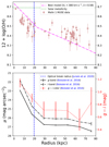 |
Fig. 8. Radial gas metallicity and stellar profile. Top: metallicity gradient in Malin 1. The brown hexagons show the extended disk regions of Malin 1 discussed in Sect. 3.3. The observed metallicities shown here are based on the Marino et al. (2013) N2 calibrator. The dot-dashed magenta line is the best-fit model of Malin 1, with a circular velocity of 380 km s−1 and a spin parameter of 0.58, obtained after a refitting following Boissier et al. (2016). Bottom: optical surface brightness profile of Malin 1 in the g- (solid black line) and i-band (dot-dashed black line) from Boissier et al. (2016). The secondary axis on the right shows the g − i color profile from Boissier et al. (2016) as the dotted red line. The stellar profiles are shown only until the radial range for which we have a metallicity estimate. The vertical dashed blue line is the i-band surface brightness break radius from Junais et al. (2020). |
A flattening in metallicity beyond the break radius9 is also observed in other galaxies, such as M 83 (Bresolin et al. 2009). Interestingly, M 83 is an XUV galaxy with a very extended UV disk. XUVs are thought to have similarities with GLSBs (Thilker et al. 2007; Bigiel et al. 2010; Hagen et al. 2016). Our observed similarities in the metallicity gradient support this hypothesis. The flattening of the metallicity beyond the break radius could have several reasons. Bresolin et al. (2009) proposed that a metallicity gradient like this could be the result of the flow of metals from the inner to the outer disk, accretion of pre-enriched gas, or past interaction with a satellite galaxy. We compared our observations in Malin 1 with the metallicity gradient from a model similar to the one shown in Boissier et al. (2016). To do this, we updated the Boissier et al. (2016) model by performing a similar fit on the photometric profiles, but with the same grid of models as in Junais et al. (2022; excluding ram pressure). We find the best parameters to be very close to the original ones:  km s−1 and
  , where VC and λ are the circular velocity and the halo spin parameters, respectively, from the models of Boissier et al. (2016). We find a difference, however, as the metallicity is much higher than in the model published in Boissier et al. (2016). For instance, at a radius of 55 kpc in Malin 1, Boissier et al. (2016) predicted a metallicity of 0.1 Z⊙, whereas the best model we obtained now has a metallicity of 0.45 Z⊙ at the same radius (see the dot-dashed magenta line in Fig. 8). After inspection, we realized that the model in Boissier et al. (2016) used the Kroupa et al. (1993) IMF while we adopted the Kroupa (2001) IMF in Junais et al. (2022). Differences in the IMF can indeed generate large differences in the net yield integrated over the IMF (e.g., Vincenzo et al. 2016). The Kroupa et al. (1993) IMF is much poorer in massive stars than that of Kroupa (2001), and therefore, the metallicity profile here is about five times higher than the one published in Boissier et al. (2016). The overall metallicity level of the model is consistent with the observations within their scatter in the inner region at ≲20 kpc (see Fig. 8), especially if we take the large systematic uncertainties of the model in the IMF and yields into account. However, the metallicity gradient of the model fails to reproduce the metallicity plateau beyond 20 kpc and is steeper than in the observations. This indicates that this simple model (in which the system evolves in isolation without radial migration) is probably insufficient to reproduce all the properties of the galaxy (see, e.g., Kubryk et al. 2013 for the effect of radial migration on chemical abundance gradients).
The bottom panel of Fig. 8 shows the radial variation in the g- and i-band optical surface brightness and color profiles of Malin 1 from Boissier et al. (2016). The correlation in the radial surface brightness and color profiles with that of the metallicity gradient shown in the top panel of Fig. 8 is clear. For both the surface brightness and color profiles, we observe a steep decline in the inner part out to ∼20 kpc, followed by a flattening. This is consistent with the trend in the metallicity. This is similar to the observation of Marino et al. (2016) for the extended disks of local spiral galaxies from the CALIFA survey. Based on the shape of the surface brightness profile, Malin 1 has an up-bending or antitruncated type III profile (Erwin et al. 2005), where the inner disk has a steeper surface brightness slope than the extended outer disk (see the bottom panel of Fig. 8). Marino et al. (2016) found that type III galaxies have a positive correlation of the change in color and metallicity gradient, followed by a flattening in metallicity. We find the same trend in Malin 1. Several scenarios have been proposed in the literature for the formation of type III profiles. Younger et al. (2007) found that minor mergers can produce type III surface brightness profiles. On the other hand, Ruiz-Lara et al. (2017) suggested that type III profiles form as a result of the radial migration of material from the inner to outer disk, as well as the through the accretion of material from the outskirts. This notion was challenged by Tang et al. (2020), who found that stellar migration alone cannot form type III profiles. Therefore, it is likely that most of the antitruncated disk of Malin 1 resulted from the accretion of material from the outskirts (e.g., pre-enriched gas from a minor merger). The flattening of the color and metallicity profiles and the rather high metallicity (0.6 Z⊙) in the extended disk also point in this direction. With the mass-metallicity scaling relations for gas and stars in isolated Local Group dwarf galaxies (see Hidalgo 2017), the outer disk gas abundance in Malin 1 would correspond to a Large Magellanic Cloud-type dwarf galaxy with a stellar and gas mass of ∼109.5 − 10 M⊙ each.
In the same way that gas metallicity traces recent star formation, photometric colors trace older stellar population ages (and abundances). The similarity of their radial profiles in Fig. 8, together with the break at 20 kpc in both, points to distinct evolutionary histories of the inner and outer galaxy systems over the epoch of the tracers, that is from billions of years in the past to the recent dozens of million years traced by the gas. This in turn means that the mechanisms of star formation and feedback or enrichment in either of the components were not significantly influenced by the other, and neither were both components altered by radial migration. In this sense, Malin 1 might be thought of as a composite galaxy with morphological subcomponents that have evolved independently over many billions of years. The quantitative implications of this scenario will be explored in future work.
The apparent correlation between the abundance and surface brightness profile also echoes the fact that abundance gradients expressed per disk scale length (Rd) tend to have a universal value with only a small scatter for disk galaxies (Prantzos & Boissier 2000; Sánchez et al. 2014). In Malin 1, we separated the inner disk (< 20 kpc) and the outer disk (> 20 kpc), as shown in Fig. 8. Junais et al. (2020) showed that the inner and outer disks of Malin 1 are separated at ∼20 kpc, with scale lengths of 5.3 kpc and 41.8 kpc, respectively. We performed separate linear fits to the abundance gradients of both disks. We found that for the inner and the outer disk, the slope of the abundance gradient normalized by its disk scale length has a value of −0.09 dex/Rd and 0.04 dex/Rd, respectively. Sánchez et al. (2014) showed that for local disk galaxies, this value is in the range of −0.06 ± 0.05 dex/Rd. Therefore, the normalized abundance gradient of the inner disk of Malin 1 has a negative value, close to the mean value found in normal galaxies. However, the outer disk is consistent with a small positive gradient, but within the 2σ scatter of Sánchez et al. (2014), suggesting that the extended disk of Malin 1 lies along the extreme tail of standard galaxies. This may indicate a particular mode of star formation at relatively low densities.
4.3. Star formation efficiency in the low-density regime
The efficiency of star formation activity in the low-density regime is often debated. LSBs are thought to have very low star formation efficiencies compared to their high surface brightness counterparts (e.g., Bigiel et al. 2008; Wyder et al. 2009). This results in the divergence of LSBs from the global Kennicutt–Schmidt law (KS relation; Kennicutt 1998) for star-forming galaxies, as shown in Fig. 9. This may be related to the possible existence of a gas density threshold (de los Reyes & Kennicutt 2019), below which star formation has a very low efficiency. The extended disks of GLSB galaxies offer a new laboratory for studying the star formation activity in this low-density regime.
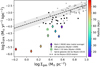 |
Fig. 9. SFR surface density vs. gas surface density. The diamonds mark the region in the disk of Malin 1 based on the radial averaged ΣSFR we estimated as in Fig. 5. The Σgas for Malin 1 is from the eight H I data points of Lelli et al. (2010), after correcting for helium by a factor of 1.4. The color bar indicates the radius throughout the disk of Malin 1. The open black circles are normal spiral galaxies from de los Reyes & Kennicutt (2019, the Σgas from de los Reyes & Kennicutt 2019 uses the total atomic and molecular gas mass). The dashed black line and the shaded gray region show the de los Reyes & Kennicutt (2019) best-fit relation and 1σ scatter. The black squares show the LSB galaxies from Wyder et al. (2009) in Malin 1. They are marked as the open green star based on the UV ΣSFR estimate from Wyder et al. (2009). |
Figure 9 shows our measured ΣSFR and gas surface density for Malin 1 at various radii of its disk. To plot this figure, we used the H I gas profile from Lelli et al. (2010), which was obtained from the Karl G. Jansky Very Large Array (VLA) data, with a resolution of ∼20″. We combined these profiles with our azimuthally averaged SFR profile from Sect. 3.2. Even though our data were only obtained in one quarter of the galaxy, we can make this comparison because the gas distribution is expected to be symmetric (see Fig. 6 of Lelli et al. 2010). At a given H I gas surface density, Σgas, the ΣSFR level of Malin 1 falls much below the level and scatter expected for normal star-forming spiral galaxies from de los Reyes & Kennicutt (2019). This indicates that star formation efficiency in the disk of Malin 1 is very low. This effect is dominant in the outermost part of the disk (r > 60 kpc), where we see a large difference of ∼2 dex in ΣSFR with respect to normal star-forming galaxies, whereas it is ∼1 dex for the inner regions. Within this region, the ΣSFR of Malin 1 is also consistent with what is observed for other LSBs and GLSBs in the literature (Boissier et al. 2008; Wyder et al. 2009; Saburova et al. 2021). Our estimates agree with the average value of ΣSFR for Malin 1 found by Wyder et al. (2009) based on the GALEX UV data. Overall, the disk of Malin 1 clearly lies along the extreme end of ΣSFR level compared to any other known LSB galaxy.
We point out that the gas surface density of normal spiral galaxies shown in Fig. 9 from de los Reyes & Kennicutt (2019) includes the total of atomic H I and molecular H2 gas, but the LSBs from Wyder et al. (2009) and our Malin 1 data points only include H I. However, it is reasonable to assume that the molecular gas fraction is negligible in LSBs and GLSBs (Braine et al. 2000; Galaz et al. 2008; Wyder et al. 2009). Moreover, any additional H2 gas in Malin 1 would move the points shown in Fig. 9 toward the right, that is, farther away from the relation for normal galaxies. Because on the one hand, we detect huge regions of young stars surrounded by ionized gas emitting in Hα, and on the other hand, no CO emission was detected in previous or in recent efforts with millimeter observations, the ISM in Malin 1 is quite peculiar. As suggested by some authors (Galaz et al. 2022, and references therein), not only could the ISM be at a very low density, as all these studies seem to indicate, but it might also have a higher temperature than the ISM observed in high surface brightness spirals. Following Boissier et al. (2004), we estimated the gas-to-dust ratio in the extended disk of Malin 1 by using the ratio of our observed V-band attenuation AV (from Eq. (1)) and the H I column density (NH) from Lelli et al. (2010). We found a mean gas-to-dust ratio of log(Mgas/Mdust) = 2.06. For our average gas metallicity of ∼0.6 Z⊙ in the extended disk, this gas-to-dust ratio is consistent with the lower limit, but within the scatter found for normal galaxies (e.g., Boissier et al. 2004; Rémy-Ruyer et al. 2014).
5. Conclusions
We presented VLT/MUSE IFU observations of the GLSB galaxy Malin 1. We extracted several ionized gas emission lines using these data and performed a detailed analysis of the SFR, dust attenuation, and gas metallicity within this galaxy. Our main results are summarized as follows.
-
For the first time, we observed strong Hα emission in numerous regions along the extended disk of Malin 1 up to a radial distance of ∼100 kpc. Other emission lines ([N II]6583, Hβ and [O III]5007) were also observed, but in fewer regions. This indicates that recent star formation is ongoing in several regions in the large diffuse disk of Malin 1.
-
We estimated the Balmer decrement and dust attenuation in several regions of the galaxy and found that the disk of Malin 1 has a mean Balmer ratio of 3.26 and an Hα attenuation of 0.36 mag, assuming case-B gas conditions. This is also true at several tens of kiloparsec from the galaxy center, where we measured it in a bright star-forming region.
-
Malin 1 has a steep decline in the SFR surface density (ΣSFR) within the inner 20 kpc, followed by a shallow decline in the extended disk. We also see a peak in ΣSFR around the 60 kpc radius. Our radial average ΣSFR estimates based on Hα are consistent with the measurements from UV as well as with other works from the literature.
-
The gas metallicity in Malin 1 shows a steep decline in the central region, similar to the radial Hα profile. However, we observe a flattening of the metallicity in the extended disk with a rather high value of about 0.6 Z⊙ within a radius range between 20 kpc and 80 kpc. We found that the outer disk abundance gradient in Malin 1, normalized by its scale length, has a value close to zero, which is flatter than that of most normal disk galaxies in the literature. The abundance measurements in these very extended regions confirm that the gas is not primordial and that the gradient is flatter than expected for very simple models. Together with similar radial trends from photometric colors, this result suggests distinct star formation histories for the inner and outer disks of Malin 1, with little radial migration or interactions at play during the formation of its very extended disk.
-
The comparison of our estimated SFR surface density and the gas surface density shows that, unlike normal spiral galaxies, Malin 1 lies in the regime of very low star formation efficiency, as found in other LSBs, but at the extreme lower limit.
This work allows us to provide new constraints on the properties and the formation of the GLSB galaxy Malin 1 from partial MUSE observations. To understand the nature of GLSBs better, we require complimentary MUSE observations for Malin 1 (covering the entire galaxy) as well as for other GLSBs.
We masked significant telluric residuals that might affect the fit, the NaD-gap created to suppress the AO laser emission, and also the atmospheric Raman features created by the lasers.
We did not perform any velocity corrections during the H II region spectral stacking discussed in Sect. 2.2.2 because the average size of a region (∼2 kpc) in that case was too small to have any significant velocity variations.
This assumes (1) optically thin gas, (2) which is ionized by a harder radiation field than produced by the recombination process itself, and (3) that there is negligible influence of the ionizing radiation on the gas temperature. See also Nebrin (2023).
We applied an attenuation correction for both the UV and the Hα radial average data using a mean AHα = 0.36 mag as obtained from Sect. 3.1.
The WISE image of Malin 1 was inspected using the Legacy Survey Viewer (https://www.legacysurvey.org/viewer).
Assuming case B recombination, i.e., optically thin gas.
The break radius of M 83 is at 8.1 kpc (Barnes et al. 2014).
Acknowledgments
J. and K.M. are grateful for support from the Polish National Science Centre via grant UMO-2018/30/E/ST9/00082. P.M.W. gratefully acknowledges support by the German BMBF from the ErUM program (project VLT-BlueMUSE, grant 05A20BAB). G.G., E.J.J., and T.H.P. gratefully acknowledge support by the ANID BASAL project FB210003. T.H.P. gratefully acknowledges support through a FONDECYT Regular grant (No. 1201016). E.J.J. acknowledges support from FONDECYT Iniciación en investigación 2020 Project 11200263. This work was partially supported by the “PHC POLONIUM” programme (project number: 49136QB), funded by the French Ministry for Europe and Foreign Affairs, the French Ministry for Higher Education and Research and by the Polish National Agency for Academic Exchange (BPN/BFR/2022/1/00005).
References
- Bacon, R., Accardo, M., Adjali, L., et al. 2010, Proc. SPIE, 7735, 773508 [Google Scholar]
- Barnes, K. L., van Zee, L., Dale, D. A., et al. 2014, ApJ, 789, 126 [NASA ADS] [CrossRef] [Google Scholar]
- Barth, A. J. 2007, AJ, 133, 1085 [NASA ADS] [CrossRef] [Google Scholar]
- Bigiel, F., Leroy, A., Walter, F., et al. 2008, AJ, 136, 2846 [NASA ADS] [CrossRef] [Google Scholar]
- Bigiel, F., Leroy, A., Walter, F., et al. 2010, AJ, 140, 1194 [NASA ADS] [CrossRef] [Google Scholar]
- Boissier, S. 2013, in Planets, Stars and Stellar Systems. Volume 6: Extragalactic Astronomy and Cosmology, eds. T. D. Oswalt, & W. C. Keel, 6, 141 [NASA ADS] [CrossRef] [Google Scholar]
- Boissier, S., Boselli, A., Buat, V., Donas, J., & Milliard, B. 2004, A&A, 424, 465 [NASA ADS] [CrossRef] [EDP Sciences] [Google Scholar]
- Boissier, S., Gil de Paz, A., Boselli, A., et al. 2008, ApJ, 681, 244 [NASA ADS] [CrossRef] [Google Scholar]
- Boissier, S., Boselli, A., Ferrarese, L., et al. 2016, A&A, 593, A126 [NASA ADS] [CrossRef] [EDP Sciences] [Google Scholar]
- Boselli, A., Fossati, M., Gavazzi, G., et al. 2015, A&A, 579, A102 [NASA ADS] [CrossRef] [EDP Sciences] [Google Scholar]
- Bothun, G. D., Impey, C. D., Malin, D. F., & Mould, J. R. 1987, AJ, 94, 23 [NASA ADS] [CrossRef] [Google Scholar]
- Braine, J., Herpin, F., & Radford, S. J. E. 2000, A&A, 358, 494 [NASA ADS] [Google Scholar]
- Bresolin, F. 2017, in Outskirts of Galaxies, eds. J. H. Knapen, J. C. Lee, & A. Gil de Paz, Astrophys. Space Sci. Lib., 434, 145 [NASA ADS] [CrossRef] [Google Scholar]
- Bresolin, F., Ryan-Weber, E., Kennicutt, R. C., & Goddard, Q. 2009, ApJ, 695, 580 [Google Scholar]
- Calzetti, D. 1997, AJ, 113, 162 [NASA ADS] [CrossRef] [Google Scholar]
- Calzetti, D., Armus, L., Bohlin, R. C., et al. 2000, ApJ, 533, 682 [NASA ADS] [CrossRef] [Google Scholar]
- Cappellari, M. 2017, MNRAS, 466, 798 [Google Scholar]
- Cappellari, M., & Copin, Y. 2003, MNRAS, 342, 345 [Google Scholar]
- Cardelli, J. A., Clayton, G. C., & Mathis, J. S. 1989, ApJ, 345, 245 [Google Scholar]
- de los Reyes, M. A. C., & Kennicutt, R. C., Jr. 2019, ApJ, 872, 16 [NASA ADS] [CrossRef] [Google Scholar]
- Domínguez, A., Siana, B., Henry, A. L., et al. 2013, ApJ, 763, 145 [CrossRef] [Google Scholar]
- Epinat, B., Tasca, L., Amram, P., et al. 2012, A&A, 539, A92 [NASA ADS] [CrossRef] [EDP Sciences] [Google Scholar]
- Erwin, P., Beckman, J. E., & Pohlen, M. 2005, ApJ, 626, L81 [Google Scholar]
- Erwin, P., Pohlen, M., & Beckman, J. E. 2008, AJ, 135, 20 [Google Scholar]
- Ferrarese, L., Côté, P., Cuillandre, J.-C., et al. 2012, ApJS, 200, 4 [Google Scholar]
- Fusco, T., Bacon, R., Kamann, S., et al. 2020, A&A, 635, A208 [NASA ADS] [CrossRef] [EDP Sciences] [Google Scholar]
- Galaz, G., Cortés, P., Bronfman, L., & Rubio, M. 2008, ApJ, 677, L13 [NASA ADS] [CrossRef] [Google Scholar]
- Galaz, G., Milovic, C., Suc, V., et al. 2015, ApJ, 815, L29 [NASA ADS] [CrossRef] [Google Scholar]
- Galaz, G., Frayer, D. T., Blaña, M., et al. 2022, ApJ, 940, L37 [NASA ADS] [CrossRef] [Google Scholar]
- Hagen, L. M. Z., Seibert, M., Hagen, A., et al. 2016, ApJ, 826, 210 [NASA ADS] [CrossRef] [Google Scholar]
- Hamed, M., Małek, K., Buat, V., et al. 2023, A&A, 674, A99 [NASA ADS] [CrossRef] [EDP Sciences] [Google Scholar]
- Hidalgo, S. L. 2017, A&A, 606, A115 [NASA ADS] [CrossRef] [EDP Sciences] [Google Scholar]
- Hinz, J. L., Rieke, M. J., Rieke, G. H., et al. 2007, ApJ, 663, 895 [NASA ADS] [CrossRef] [Google Scholar]
- Impey, C., & Bothun, G. 1997, ARA&A, 35, 267 [NASA ADS] [CrossRef] [Google Scholar]
- Ivezić, Ž., Kahn, S. M., Tyson, J. A., et al. 2019, ApJ, 873, 111 [Google Scholar]
- Junais 2021, PhD Thesis, Astrophysique et cosmologie Aix-Marseille, France [Google Scholar]
- Junais, Boissier, S., Epinat, B., et al. 2020, A&A, 637, A21 [NASA ADS] [CrossRef] [EDP Sciences] [Google Scholar]
- Junais, Boissier, S., Boselli, A., et al. 2022, A&A, 667, A76 [NASA ADS] [CrossRef] [EDP Sciences] [Google Scholar]
- Junais, Małek, K., Boissier, S., et al. 2023, A&A, 676, A41 [NASA ADS] [CrossRef] [EDP Sciences] [Google Scholar]
- Kennicutt, R. C., Jr. 1998, ApJ, 498, 541 [Google Scholar]
- Kewley, L. J., & Ellison, S. L. 2008, ApJ, 681, 1183 [Google Scholar]
- Kotulla, R., Fritze, U., Weilbacher, P., & Anders, P. 2009, MNRAS, 396, 462 [NASA ADS] [CrossRef] [Google Scholar]
- Kroupa, P. 2001, MNRAS, 322, 231 [NASA ADS] [CrossRef] [Google Scholar]
- Kroupa, P., Tout, C. A., & Gilmore, G. 1993, MNRAS, 262, 545 [NASA ADS] [CrossRef] [Google Scholar]
- Kubryk, M., Prantzos, N., & Athanassoula, E. 2013, MNRAS, 436, 1479 [NASA ADS] [CrossRef] [Google Scholar]
- Lelli, F., Fraternali, F., & Sancisi, R. 2010, A&A, 516, A11 [NASA ADS] [CrossRef] [EDP Sciences] [Google Scholar]
- Liang, Y. C., Zhong, G. H., Hammer, F., et al. 2010, MNRAS, 409, 213 [NASA ADS] [CrossRef] [Google Scholar]
- Lin, Z., & Kong, X. 2020, ApJ, 888, 88 [NASA ADS] [CrossRef] [Google Scholar]
- Lindegren, L., Klioner, S. A., Hernández, J., et al. 2021, A&A, 649, A2 [EDP Sciences] [Google Scholar]
- López-Sánchez, Á. R., Westmeier, T., Esteban, C., & Koribalski, B. S. 2015, MNRAS, 450, 3381 [CrossRef] [Google Scholar]
- Marino, R. A., Rosales-Ortega, F. F., Sánchez, S. F., et al. 2013, A&A, 559, A114 [NASA ADS] [CrossRef] [EDP Sciences] [Google Scholar]
- Marino, R. A., Gil de Paz, A., Sánchez, S. F., et al. 2016, A&A, 585, A47 [NASA ADS] [CrossRef] [EDP Sciences] [Google Scholar]
- Martin, G., Kaviraj, S., Laigle, C., et al. 2019, MNRAS, 485, 796 [NASA ADS] [CrossRef] [Google Scholar]
- Matthews, L. D., van Driel, W., & Monnier-Ragaigne, D. 2001, A&A, 365, 1 [NASA ADS] [CrossRef] [EDP Sciences] [Google Scholar]
- Micheva, G., Roth, M. M., Weilbacher, P. M., et al. 2022, A&A, 668, A74 [NASA ADS] [CrossRef] [EDP Sciences] [Google Scholar]
- Moore, L., & Parker, Q. A. 2006, PASA, 23, 165 [NASA ADS] [CrossRef] [Google Scholar]
- Munari, U., Sordo, R., Castelli, F., & Zwitter, T. 2005, A&A, 442, 1127 [NASA ADS] [CrossRef] [EDP Sciences] [Google Scholar]
- Nebrin, O. 2023, Res. Notes Am. Astron. Soc., 7, 90 [Google Scholar]
- Osterbrock, D. E. 1989, Astrophysics of Gaseous Nebulae and Active Galactic Nuclei (Mill Valley: University Science Books) [Google Scholar]
- Pickering, T. E., Impey, C. D., van Gorkom, J. H., & Bothun, G. D. 1997, AJ, 114, 1858 [NASA ADS] [CrossRef] [Google Scholar]
- Prantzos, N., & Boissier, S. 2000, MNRAS, 313, 338 [NASA ADS] [CrossRef] [Google Scholar]
- Rahman, N., Howell, J. H., Helou, G., Mazzarella, J. M., & Buckalew, B. 2007, ApJ, 663, 908 [NASA ADS] [CrossRef] [Google Scholar]
- Rémy-Ruyer, A., Madden, S. C., Galliano, F., et al. 2014, A&A, 563, A31 [Google Scholar]
- Ruiz-Lara, T., Few, C. G., Florido, E., et al. 2017, A&A, 608, A126 [NASA ADS] [CrossRef] [EDP Sciences] [Google Scholar]
- Saburova, A. S., Chilingarian, I. V., Kasparova, A. V., et al. 2021, MNRAS, 503, 830 [NASA ADS] [CrossRef] [Google Scholar]
- Saburova, A. S., Chilingarian, I. V., Kulier, A., et al. 2023, MNRAS, 520, L85 [Google Scholar]
- Saha, K., Dhiwar, S., Barway, S., Narayan, C., & Tandon, S. 2021, JApA, 42, 59 [NASA ADS] [Google Scholar]
- Sánchez, S. F., Rosales-Ortega, F. F., Iglesias-Páramo, J., et al. 2014, A&A, 563, A49 [CrossRef] [EDP Sciences] [Google Scholar]
- Schlegel, D. J., Finkbeiner, D. P., & Davis, M. 1998, ApJ, 500, 525 [Google Scholar]
- Schombert, J., McGaugh, S., & Maciel, T. 2013, AJ, 146, 41 [NASA ADS] [CrossRef] [Google Scholar]
- Sprayberry, D., Impey, C. D., Bothun, G. D., & Irwin, M. J. 1995, AJ, 109, 558 [NASA ADS] [CrossRef] [Google Scholar]
- Ströbele, S., La Penna, P., Arsenault, R., et al. 2012, in Adaptive Optics Systems III, eds. B. L. Ellerbroek, E. Marchetti, & J. P. Véran, SPIE Conf. Ser., 8447, 844737 [CrossRef] [Google Scholar]
- Subramanian, S., Ramya, S., Das, M., et al. 2016, MNRAS, 455, 3148 [NASA ADS] [CrossRef] [Google Scholar]
- Tang, Y., Chen, Q., Zhang, H.-X., et al. 2020, ApJ, 897, 79 [NASA ADS] [CrossRef] [Google Scholar]
- Thilker, D. A., Bianchi, L., Meurer, G., et al. 2007, ApJS, 173, 538 [Google Scholar]
- Vazdekis, A., Koleva, M., Ricciardelli, E., Röck, B., & Falcón-Barroso, J. 2016, MNRAS, 463, 3409 [Google Scholar]
- Vincenzo, F., Matteucci, F., Belfiore, F., & Maiolino, R. 2016, MNRAS, 455, 4183 [Google Scholar]
- Weilbacher, P. M., Monreal-Ibero, A., Verhamme, A., et al. 2018, A&A, 611, A95 [NASA ADS] [CrossRef] [EDP Sciences] [Google Scholar]
- Weilbacher, P. M., Palsa, R., Streicher, O., et al. 2020, A&A, 641, A28 [NASA ADS] [CrossRef] [EDP Sciences] [Google Scholar]
- Wyder, T. K., Martin, D. C., Barlow, T. A., et al. 2009, ApJ, 696, 1834 [NASA ADS] [CrossRef] [Google Scholar]
- Younger, J. D., Cox, T. J., Seth, A. C., & Hernquist, L. 2007, ApJ, 670, 269 [NASA ADS] [CrossRef] [Google Scholar]
- Yuan, F.-T., Argudo-Fernández, M., Shen, S., et al. 2018, A&A, 613, A13 [NASA ADS] [CrossRef] [EDP Sciences] [Google Scholar]
Appendix A: Table of measurements
Properties of the Hα selected regions in the extended disk of Malin 1 as discussed in Sect. 2.2.2.
All Tables
Properties of the Hα selected regions in the extended disk of Malin 1 as discussed in Sect. 2.2.2.
All Figures
|
Fig. 1. Color-composite image of Malin 1 from the Canada-France-Hawaii Telescope (CFHT) Megacam NGVS survey u-, g-, and i-band images (Ferrarese et al. 2012). The image spans a width of ∼2.6′×2.6′. The red box shows the MUSE field of observation (1′×1′). |
| In the text | |
|
Fig. 2. Emission line flux maps of the central region of Malin 1 (21″ × 21″) obtained from the pPXF fitting. The Hα and the Hβ lines are shown in the top panels, and the [N II]6583 and the [O III]5007 lines are shown in the bottom panels. The color bar indicates the flux corresponding to each line. |
| In the text | |
|
Fig. 3. Emission line flux maps of Malin 1 obtained from the pPXF fitting of the H II regions. The Hα, and the Hβ lines are shown in the top panels, and the [N II]6583 and the [O III]5007 lines are shown in the bottom panels. The ID of each region, as discussed in Sect. 2.2.2, is labeled in black in the top left panel. The regions with ID 27 and 49 are excluded from the maps as they do not have an S/N > 2.5 in any of the emission lines. The color bar indicates the flux corresponding to each emission line. The flux value of each region is given as the average flux per pixel within that region obtained from the fitting of its row-stacked spectrum. |
| In the text | |
|
Fig. 4. Radial variation of the Balmer ratio (left panel) and Hα attenuation (right panel). The blue circles and the brown hexagons show the central regions and the extended disk regions, respectively, obtained from the pPXF fit discussed in Sect. 2.2. The horizontal dashed red line marks the intrinsic Balmer ratio of 2.86 for case B recombination. To all regions in which the Balmer ratio was below this value, we assigned zero attenuation. The histograms next to each panel give the overall distribution of each quantity (the solid blue line and the dashed brown line show the central region and extended disk, respectively). Their mean values are indicated at the top of each panel. |
| In the text | |
|
Fig. 5. SFR surface density of Malin 1 as a function of galactocentric radius. The blue circles and brown hexagons show the central regions and the extended disk regions, respectively, obtained from the pPXF fit discussed in Sect. 2.2. The red diamonds are the Hα radial average measured in concentric rings with a width of 5″ from the center. The orange stars show the radial averages measured in the same field in the UVIT FUV image of Malin 1 from Saha et al. (2021), as shown in Fig. 6. For illustration purposes, the UV data points are horizontally shifted by 2 kpc. The green squares show the data points from Junais et al. (2020), based on the IMACS-Magellan Hα long-slit spectra of Malin 1. |
| In the text | |
|
Fig. 6. FUV image of Malin 1 from Saha et al. (2021) of the same field as our MUSE observations (shown as the red box). The green contours mark the Hα-detected regions, as discussed in Sect. 2.2.2. |
| In the text | |
|
Fig. 7. Radial variation of the metallicity of Malin 1. Left: metallicity using the N2 calibrator of Marino et al. (2013). Right: metallicity using the O3N2 calibrator of Marino et al. (2013). The blue circles and brown hexagons show the central regions and extended disk regions, respectively, as discussed in Sect. 2.2. The horizontal dotted green line marks the solar metallicity. The uncertainty of the N2 and O3N2 calibrations from Marino et al. (2013) is 0.16 dex and 0.18 dex, respectively. |
| In the text | |
|
Fig. 8. Radial gas metallicity and stellar profile. Top: metallicity gradient in Malin 1. The brown hexagons show the extended disk regions of Malin 1 discussed in Sect. 3.3. The observed metallicities shown here are based on the Marino et al. (2013) N2 calibrator. The dot-dashed magenta line is the best-fit model of Malin 1, with a circular velocity of 380 km s−1 and a spin parameter of 0.58, obtained after a refitting following Boissier et al. (2016). Bottom: optical surface brightness profile of Malin 1 in the g- (solid black line) and i-band (dot-dashed black line) from Boissier et al. (2016). The secondary axis on the right shows the g − i color profile from Boissier et al. (2016) as the dotted red line. The stellar profiles are shown only until the radial range for which we have a metallicity estimate. The vertical dashed blue line is the i-band surface brightness break radius from Junais et al. (2020). |
| In the text | |
|
Fig. 9. SFR surface density vs. gas surface density. The diamonds mark the region in the disk of Malin 1 based on the radial averaged ΣSFR we estimated as in Fig. 5. The Σgas for Malin 1 is from the eight H I data points of Lelli et al. (2010), after correcting for helium by a factor of 1.4. The color bar indicates the radius throughout the disk of Malin 1. The open black circles are normal spiral galaxies from de los Reyes & Kennicutt (2019, the Σgas from de los Reyes & Kennicutt 2019 uses the total atomic and molecular gas mass). The dashed black line and the shaded gray region show the de los Reyes & Kennicutt (2019) best-fit relation and 1σ scatter. The black squares show the LSB galaxies from Wyder et al. (2009) in Malin 1. They are marked as the open green star based on the UV ΣSFR estimate from Wyder et al. (2009). |
| In the text | |
Current usage metrics show cumulative count of Article Views (full-text article views including HTML views, PDF and ePub downloads, according to the available data) and Abstracts Views on Vision4Press platform.
Data correspond to usage on the plateform after 2015. The current usage metrics is available 48-96 hours after online publication and is updated daily on week days.
Initial download of the metrics may take a while.