| Issue |
A&A
Volume 676, August 2023
|
|
|---|---|---|
| Article Number | A90 | |
| Number of page(s) | 14 | |
| Section | Catalogs and data | |
| DOI | https://doi.org/10.1051/0004-6361/202245564 | |
| Published online | 11 August 2023 | |
The GAPS programme at TNG
XLIV. Projected rotational velocities of 273 exoplanet-host stars observed with HARPS-N★,★★
1
INAF – Osservatorio Astronomico di Brera,
Via E. Bianchi, 46,
23807
Merate (LC), Italy
e-mail: monica.rainer@inaf.it
2
INAF – Osservatorio Astronomico di Padova,
Vicolo dell’Osservatorio, 5,
35122
Padova (PD), Italy
3
INAF – Osservatorio Astrofisico di Torino,
Via Osservatorio 20,
10025
Pino Torinese (TO), Italy
4
Department of Astronomy, University of Geneva,
Chemin Pegasi 51,
1290
Versoix, Switzerland
5
INAF – Osservatorio Astronomico di Roma,
Via Frascati 33,
00078
Monte Porzio Catone (Roma), Italy
6
INAF – Osservatorio Astrofisico di Catania,
Via S.Sofia 78,
95123
Catania, Italy
7
INAF - Osservatorio Astronomico di Palermo,
Piazza del Parlamento, 1,
90134
Palermo, Italy
8
Instituto de Astrofísica de Canarias (IAC),
38205
La Laguna, Tenerife, Spain
9
INAF – Osservatorio Astronomico di Capodimonte,
via Moiariello 16,
80131
Napoli, Italy
10
Université Côte d’Azur, Observatoire de la Côte d’Azur, CNRS, Laboratoire Lagrange,
Bd de l’Observatoire,
CS34229,
06304
Nice Cedex 4, France
11
Department of Physics, University of Rome “Tor Vergata”,
Via della Ricerca Scientifica 1,
00133
Rome, Italy
12
Max Planck Institute for Astronomy,
Königstuhl 17,
69117
Heidelberg, Germany
13
Aix Marseille Univ, CNRS, CNES, LAM,
Marseille, France
14
INAF – Osservatorio Astronomico di Trieste,
via Tiepolo 11,
34143
Trieste, Italy
15
INAF – Fundación Galileo Galilei,
Rambla José Ana Fernandez Pérez 7,
38712
Breña Baja (TF), Spain
16
INAF – Osservatorio Astronomico di Cagliari,
via della Scienza 5,
09047
Selargius (CA), Italy
Received:
28
November
2022
Accepted:
22
June
2023
Context. The leading spectrographs used for exoplanets’ search and characterization offer online data reduction softwares (DRS) that yield, as an ancillary result, the full-width at half-maximum (FWHM) of the cross-correlation function (CCF) that is used to estimate the radial velocity of the host star. The FWHM also contains information on the stellar projected rotational velocity veq sin i★, if appropriately calibrated.
Aims. We wanted to establish a simple relationship to derive the veq sin i★ directly from the FWHM computed by the HARPS-N DRS in the case of slow-rotating solar-like stars. This may also help to recover the stellar inclination i★, which in turn affects the exoplanets’ parameters.
Methods. We selected stars with an inclination of the spin axis compatible with 90 deg by looking at exoplanetary transiting systems with known small sky-projected obliquity: for these calibrators, we can presume that veq sin i★ is equal to stellar equatorial velocity veq. We derived their rotational periods from photometric and spectroscopic time series and their radii from the spectral energy distribution (SED) fitting. This allowed us to recover their veq, which could be compared to the FWHM values of the CCFs obtained both with G2 and K5 spectral-type masks.
Results. We obtained an empirical relation for each mask: this can be used to derive veq sin i★ directly from FWHM values for slow rotators (FWHM < 20 km s−1). We applied our relations to 273 exoplanet-host stars observed with HARPS-N, obtaining homogeneous veqsin i★ measurements. When possible, we compared our results with the literature ones to confirm the reliability of our work. We were also able to recover or constrain i★ for 12 objects with no prior veq sin i★ estimation.
Conclusions. We provide two simple empirical relations to directly convert the HARPS-N FWHM obtained with the G2 and K5 mask to a veq sin i★ value. We tested our results on a statistically significant sample, and we found a good agreement with literature values found with more sophisticated methods for stars with log ɡ > 3.5. We also tried our relation on HARPS and SOPHIE data, and we conclude that it can be used as it is also on FWHM derived by HARPS DRS with the G2 and K5 mask, and it may be adapted to the SOPHIE data as long as the spectra are taken in high-resolution mode.
Key words: planetary systems / techniques: spectroscopic / stars: rotation
Full Table 4 is only available at the CDS via anonymous ftp to cdsarc.cds.unistra.fr (130.79.128.5) or via https://cdsarc.cds.unistra.fr/viz-bin/cat/J/A+A/676/A90
© The Authors 2023
 Open Access article, published by EDP Sciences, under the terms of the Creative Commons Attribution License (https://creativecommons.org/licenses/by/4.0), which permits unrestricted use, distribution, and reproduction in any medium, provided the original work is properly cited.
This article is published in open access under the Subscribe to Open model. Subscribe to A&A to support open access publication.
1 Introduction
Stable, high-resolution (HR) optical spectrographs are some of the leading instruments used for the search and characterization of the exoplanets: many of them are designed expressly for these studies (e.g. HARPS, HARPS-N, ESPRESSO), and as such they are equipped with dedicated data reduction softwares (DRS). One of the main deliverables of the DRS is the cross-correlation function (CCF) of the reduced spectra with a stellar mask chosen from the available library of spectral-type templates (Baranne et al. 1996; Pepe et al. 2002).
The CCF allows for the radial velocity of the host star to be computed with a very high precision, and it also yields a number of additional parameters, such as the CCF’s bisector span (which can be used as an activity indicator), the CCF’s contrast, and the full-width at half-maximum (FWHM). The latter may be related to the stellar projected rotational velocity veq sin i★ if appropriately calibrated: in this paper, we present the work done to calibrate the FWHM of the CCF that was computed by the HARPS-N DRS (Cosentino et al. 2014) using the G2 and K5 stellar masks. HARPS-N is the HR optical spectrograph installed at the Telescopio Nazionale Galileo (TNG) at the Roque de Los Muchachos Observatory (La Palma, Canary Islands, Spain).
The use of the CCF’s FWHM to estimate the veq sin i★ is particularly important in the case of slowly rotating stars, for which the veq sin i★ computation via Fourier transform of the line profiles or fitting with a rotational profile is complicated by the combination of rotational broadening with the effects of resolution smearing (≈2.6 km s−1 in the case of HARPS-N, R = 115 000), and the micro- (umicro) and macro- (umacro) turbulence broadening. Slowly rotating solar-like and M-type stars are also among the main targets in the exoplanet field; therefore, it is particularly important to have a reliable method to estimate the veq sin i★ for these objects in order to better characterize the host stars. Using the FWHM given by the HARPS-N DRS allows everyone to recover the veq sin i★ values directly for the HARPS-N archival data.
Once it is obtained, the veq sin i★ value may be used along with estimates of the stellar rotational period Prot (for example from photometric time series or spectroscopic time series of activity indices) and the stellar radius R★ – derived for example from spectral energy distribution (SED) fitting (see Sect. 2) – to recover the stellar inclination i★:
 (1)
(1)
The stellar inclination heavily affects exoplanets’ parameters (Hirano et al. 2014). Having an estimate of its value is also a fundamental step in computing the spin-orbit angle of exoplanetary systems, which is an important observational probe of the origin and evolution of the systems (e.g. Queloz et al. 2000; Winn et al. 2005).
The approach of exploiting known stellar radii and rotational periods to infer the rotational velocity and to calibrate the width of the CCF versus veq sin i★ is not completely new, as it was previously adopted by Nordström et al. (2004). However, in their case, the stellar inclination remained unknown and the additional uncertainty was treated statistically. Instead, in our work we took advantage of the known viewing geometry of stars that host a transiting planet with an orbit inclination close to 90 deg, and a good spin-orbit alignment as inferred by the measurement of the Rossiter-McLaughlin effect (Rossiter 1924; McLaughlin 1924). This allowed us to rely on a sample of objects for which the projected rotational velocity, linked to the CCF width, is similar to the equatorial velocity inferred from the rotational period and the stellar radius. Furthermore, the selection of a sample of transiting planets ensures the availability of high-quality photometric data (which were taken for the planet search itself) and in most cases of additional relevant literature studies from follow-up observations.
This paper is organized as follows: in Sect. 2 we describe the selection procedure for our calibrators. For Sect. 3, we used them to create our empirical relation, and then we applied that to a large set of exoplanet host stars in Sect. 4. We test the applicability of our relation to other spectrographs in Sect. 5, and finally we present our conclusions in Sect. 6.
2 Calibrators’ selection and characterization
To calibrate our empirical relation as accurately as possible, we relied on a very strict selection of calibrators. We queried the NASA exoplanet archive1 to obtain a list of all known exo-planet host stars with a) a declination >−25 deg (to ensure they were observable with the TNG), and b) an absolute value of the system sky-projected obliquity λ smaller than 30 deg, as derived from the Rossiter-McLaughlin effect and reported in the TEPCat catalogue (Southworth 2011). The latter value is a compromise between the need to have systems that can be considered aligned in such a way that the stellar projected rotational velocity veq sin i★ can be considered approximately equal to the stellar equatorial velocity veq, and the need to have a good number of useful calibrators (at least some tens of objects).
This selection resulted in a list of 66 targets. We then searched the TNG archive for public HARPS-N spectra of these stars, to combine them with the proprietary data obtained within the Global Architecture of Planetary Systems (GAPS) program, which is an Italian project dedicated to the search and characterization of exoplanets (PI G. Micela; Covino et al. 2013). We thus found 44 stars with useful HARPS-N CCFs.
The stellar masks available in the DRS library are optimized for main sequence stars with stellar types G2, K5, and M2. With the new upgrades to the DRS, more masks are starting to be available for different spectral types, and they will have to be calibrated accordingly. However, in this work, we focus on the original masks that have been used so far, and that are still available in the DRS. Unfortunately, the M2 CCFs are useless for our purposes because the use of the M2 mask results in deformed CCF profiles with large bumps in the wings. In a previous work (Rainer et al. 2020), we created an improved M-type mask to overcome this problem, but we do not consider this mask here because it is not publicly available: our scope is to enable astronomers to use the public HARPS-N archival data. Thus, we focus on the G2 and K5 CCFs: while this optimized our work for solar-like stars, some M-type stars may still be reduced using the K5 mask in order to recover the veq sin i★ estimate from the CCF FWHM.
Our selection criteria ensure that sin i★ ≈ 1, which means that we can consider veq sin i★ ≈ veq for all our calibrators. If we are able to estimate the equatorial velocity veq, then we can build a relation between FWHM and veq sin i★ in a straightforward way. In order to compute veq, we needed estimates of the rotational periods Prot and the radii R★ of our calibrators:
 (2)
(2)
We derived the rotation period Prot mainly from the photometry of the Transiting Exoplanet Survey Satellite (TESS) space mission (Ricker et al. 2015) and the ground-based Super Wide Angle Search for Planets (SuperWASP) project (Butters et al. 2010). In the case of TESS, we used the Pre-search Data Conditioned Simple Aperture Photometry (PDCSAP) light curves (Stumpe et al. 2012) as downloaded from the Mikulski Archive for Space Telescopes2 (MAST), where systematic artefacts are likely removed by the PDCSAP pipeline. PDCSAP light curves were analysed using the generalized Lomb-Scargle (GLS) periodogram (Zechmeister & Kürster 2009) and the detected periods are listed in Table 1. In the case of the SuperWASP photometric time series, we first disregarded possible outliers, that is data points that deviated more than three standard deviations from the mean of the whole data series. Then, we computed a filtered version of the light curve by means of a sliding median boxcar filter with a boxcar extension equal to 2 h. This filtered light curve was then subtracted from the original light curve, and all the points deviating more than three standard deviations from the residuals were discarded. Finally, we computed normal points by binning the data on time intervals having the duration of about 2 h. The rotation period search was performed by using the GLS and the CLEAN (Roberts et al. 1987) periodogram analysis. All the periodicities detected by GLS, with a false alarm probability smaller than 0.1% (see Horne & Baliunas 1986), and recovered with the same value within the uncertainty, also by CLEAN, were considered as the star’s rotation period and listed in Table 1. To compute the error associated with the period, we followed the method used by Lamm et al. (2004).
We also checked the spectroscopic activity indicators’ time series: we investigated the  activity index using GLS. In general, we did not find any conclusive results given that for most stars only a small number of observations sparsely obtained over a few years were available. In a few cases, the periodogram analysis provided Prot detection, which was always consistent with the photometrically determined period. For the sake of sample homogeneity, we thus considered only the photometric periods.
The stellar radii R★ were obtained by fitting the SED via the MESA Isochrones and Stellar Tracks (MIST, Dotter 2016; Choi et al. 2016) through the EXOFASTv2 suite (Eastman et al. 2019). Specifically, we fitted the available archival magnitudes of each star in the sample imposing Gaussian priors on the effective temperature Teff and metallicity [Fe/H] based on the respective literature values listed in Table 1 and on the parallax π based on the Gaia EDR3 astrometric measurement (Gaia Collaboration 2016, 2021). Since the SED primarily constrains R★ and Teff, the stellar parameters are simultaneously constrained by the SED and the MIST isochrones, and a penalty for straying from the MIST evolutionary tracks ensures that the resulting star realization is physical in nature (see Eastman et al. 2019, for more details on the method). In Fig. 1 we show our results compared with the R★ and Teff of the exoplanet-host stars present in the NASA archive, while in Fig. 2 we show the correlation and residuals between our values and those from the literature.
We also checked the literature for asteroseismic and interfer-ometric radii, which we found for HD 17156 (asteroseismic R★ = 1.5007 ± 0.0076 R⊙, Nutzman et al. 2010), as well as HD 189733 and HD 209458 (interferometric R★ 0.805 ± 0.016 and 1.203 ± 0.06 R⊙, respectively, Boyajian et al. 2014). We note that they are in good agreement with our results.
Thus we obtained our semi-final calibrators’ list, which is shown in Table 1: 27 stars with known Prot and R★. In the end, all our calibrators have λ < 21.2 degrees, strengthening our assumption of veq ≈ veq sin i★.
We also checked the Gaia DR3 archive to ensure that we are working with single stars: K2-29 has a fainter companion separated by ≈4.4 arcsec with ΔV = 1.8, and TrES-4 has a fainter companion separated by ≈1.6 arcsec with ΔV = 4.9. We considered that in both cases the combination of the faintness and the distance of the companions allowed us to keep the stars in our calibrators’ list.
Using the stellar parameters Teff and log ɡ from the literature, we estimated the micro- (vmicro) and macro- (vmacro) turbulence velocities for each object. In particular, vmicro was obtained with Adibekyan et al. (2012) relationships that are valid for stars with 4500 < Teff < 6500 K, 3.0 < log ɡ < 5.0, and −1.4 < [Fe/H] < 0.5 dex. Regarding vmacro, it was computed with the calibration obtained by Doyle et al. (2014) using asteroseismic rotational velocities for the stars with Teff > 5700 K, while for the stars with Teff < 5700 K we used the empirical relationship by Brewer et al. (2016). Both relations are valid for dwarf stars (see also Biazzo et al. 2022). To estimate the errors on our vmicro and vmacro, we considered the root-mean-square (rms) error given in the papers, which is larger than the errors derived from the parameters. The rms values are 0.18 km s−1 for vmicro, 0.73 km s−1 for vmicro from Doyle et al. (2014) (Teff > 5700 K), and 0.5 km s−1 for vmicro from Brewer et al. (2016) (Teff < 5700 K).
We note that HAT-P-2 has Prot = 2.82 ± 0.05 days from TESS photometry, but a completely different value from Super-WASP (97 ± 10 days). Applying Eq. (2), the TESS value yields veq = 30.12 km s−1, and the SuperWASP value veq = 0.88 km s−1. The TESS value is nearer to the veq sin i★ = 20.12 + 0.9 km s−1 result obtained from the Fourier transform of the CCF and with the 20.8 + 0.03 km s−1 value from the literature (Bonomo et al. 2017), but there is still a large discrepancy. In any case, this fast rotation excludes this star from being a useful calibrator (see Sect. 3): the final calibrators’ list thus contains the stars in Table 1 with the exception of HAT-P-2.
Calibrators.
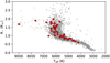 |
Fig. 1 Comparison in the Teff-R★ parameter space between the sample of stars analysed in this work (red circles) and the currently known exoplanet-host stars (grey dots) as retrieved from the NASA Exoplanet Catalog. |
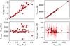 |
Fig. 2 Comparison of the stellar radii and effective temperatures obtained via the SED fitting described in Sect. 2 with literature values. Upper panels: correlations’ plot between our values and the literature ones for R★ (left panel) and Teff (right panel). Lower panels: residual plots showing the difference between our values and the literature ones. |
3 Creating the empirical relation
In order to create our empirical relation, we used as inputs the FWHM of the CCFs of the HARPS-N spectra (as computed by the HARPS-N DRS and stored in the keyword HIERARCH TNG DRS CCF FWHM of the CCF FITS files), the stellar radii R★ from Table 1, the rotational periods Prot from Table 1, and the vmicro and vmacro values from Table 1.
Using the archival CCFs, we are limited by the standard CCF half window of the HARPS-N DRS (20 km s−1): while it may be manually changed, the majority of the archival data have this value. We also note that a more precise veq sin i★ could be recovered for faster rotating stars using rotational fitting or the Fourier transform method, instead of any empirical relation. We thus limited the applicability range of our relation to FWHM up to 20 km s−1, which is a slightly larger value than the maximum FWHM that can be reliably computed with a half window of 20 km s−1, that is ≈ 16–18 km s−1.
To check this applicability range, we built a range of synthetic CCF profiles by convolving a Gaussian function with the same FWHM of the HARPS-N resolution (≈2.6 km s−1) with different rotational profiles (veq sin ranging from 0.2 to 50 km s−1 with a step of 0.2 km s−1). The rotational profiles were built using the following equation from Gray (2008):
![$f\left( x \right) = 1 - a{{2\left( {1 - a} \right)\sqrt {1 - {{\left( {{{x - {x_0}} \over {{x_l}}}} \right)}^2}} + 0.5\pi u\,\left[ {1 - {{\left( {{{x - {x_0}} \over {{x_l}}}} \right)}^2}} \right]} \over {\pi {x_l}\,\left( {1 - {u \over 3}} \right)}},$](/articles/aa/full_html/2023/08/aa45564-22/aa45564-22-eq4.png) (3)
(3)
where a is the depth of the profile, x0 the centre (i.e. the radial-velocity value), xl the veq sin of the star, and u the linear limb darkening (LD) coefficient, which we kept fixed as u = 0.6.
We fitted the resulting profiles with a Gaussian (see Fig. 3) and compared the Gaussian FWHM with the input veq sin to check their correlation. We chose a Gaussian fit to be consistent with HARPS-N DRS, which recovers both the radial velocity and the FWHM with a Gaussian fit of the CCF.
Using a single fit for the whole range resulted in some discrepancy at the borders, in particular for low FWHM values (FWHM < 6.5 km s−1), that is the range we are more interested in (see Fig. 4). As such we decided to try and improve the fit at lower values and limit our FWHM fitting range to 0–20 km s−1: in this case, while higher-order polynomials behave well enough down to FWHM = 5 km s−1, the linear fit residuals lie below 5% down to FWHM = 3.5 km s−1 (see Fig. 5). Considering that we have a small sample of calibrators (which hinders our ability to constrain a high degree polynomial), and that the linear fit recovers the veq sin i★ values with a 5% error at worst, we can then reasonably assume that using a linear fit on the calibrators with FWHM < 20 km s−1 would give us useful results. Taking all of the previous considerations into account, such as the default half-window value of the CCFs, the aim to optimize the FWHM-veq sin i★ relation for the lower FWHM values, and above all the small sample of calibrators of which only one object (HAT-P-2) has FWHM > 20 km s−1, we then excluded HAT-P-2 from the final calibrators’ list and consider our work reliably applicable only for FWHM < 20 km s−1.
The simple test done with our simulated CCFs does not take all of the other non-constant causes of broadening into account: for example, the effects of vmicro and vmacro, which highly depend on the stellar type, are not considered. A more detailed test would involve studying the CCFs obtained on a range of synthetic spectra with different veq sin i★ and stellar parameters; unfortunately, the HARPS-N DRS works only on real raw HARPS-N data, so we cannot perform this analysis. However, we were still able to test our final results in this sense, because while our calibrators’ sample is quite small, the total number of stars for which we computed veq sin i★, and that have literature values of veq sin i★ to compare them to, is large enough to allow us to look for trends or misbehaviour related to the stellar parameters (see Sect. 4).
We created our relation first by using the CCFs computed with the G2 mask, and then we repeated the work described hereafter also for the K5 CCFs. We built four data sets: (a) the original FWHM computed by the DRS (FWHMDRS); (b) the FWHMDRS minus the vmicro broadening (FWHMmic); (c) the FWHMDRS minus the vmacro broadening (FWHMmac); (d) and the FWHMDRS minus both vmicro and vmacro broadening (FWHMmic+mac). We also considered removing the instrumental broadening, but since this is a constant effect in HARPS-N spectra it is simply included in the empirical relation. The values of FWHMmic, FWHMmac, and FWHMmic+mac are obtained with the following equations:
 (4)
(4)
 (5)
(5)
 (6)
(6)
We fitted a linear relation to each one of our four data sets (Fig. 6): (a) FWHMDRS versus veq, (b) FWHMmic versus veq, (c) FWHM mac versus veq, and (d) FWHMmic+mac versus veq. The three leftmost points (TrES-4, Kepler-25, and HAT-P-8 from lower to higher FWHM, respectively) may appear as outliers, but we decided to keep them for several reasons: there are very few calibrators with FWHM > 10 km s−1, we have no solid reason to mistrust the Prot and R★ values used in our work, and the veq sin i★ computed with the resulting calibrations for hundreds of exoplanet-host stars agree well with the literature values (see Sect. 4).
As final relation, we used the most simple and straightforward one, which links the FWHMDRS as it is and the veq sin i★ linearly (Fig. 6, upper left panel), as this is the relation that may be more widely useful because it does not depend on knowledge of vmicro and vmacro. The resulting calibrations using the G2 and K5 masks are thus
 (7)
(7)
respectively.
For completeness’ sake, here, we also provide the calibrations obtained for FWHMmic (Eq. (8)), FWHMmac (Eq. (9)), and FWHMmic+mac (Eq. (10)):
 (8)
(8)
 (9)
(9)
 (10)
(10)
To estimate the errors on our veq sin i★ measurements, we applied error propagation theory. Considering that all our equations are linear fits structured as veq sin i★ = aFWHM + b, we could derive the error on veq sin i★ using the following equation:
 (11)
(11)
where σa and σb, are the uncertainties in the fit parameters, while ρ(a, b) is the correlation coefficient,
 (12)
(12)
The values of σa, σb, and ρ(a, b) for all the Eqs. (7)–(10) are listed in Table 2. We have no estimate for the error of FWHMDRS because unfortunately this information is not stored in the header of the FITS files, but we tried to recover it by checking the standard deviation of the FWHMDRS values when more than one CCF was available. We found a standard deviation of the order of 4%, which is much lower than the other contributions to the error budget. Thus we deemed Eq. (11) sufficient to estimate the errors in veqsin i★ derived from Eq. (7). Concerning Eqs. (8)–(10) instead, the error on vmicro and vmacro is expected to propagate on the FWHM, resulting in the FWHM errors  ,
,  , and
, and  . The total error whould then be the following:
 (13)
(13)
As stated before, we used the rms as errors on vmicro and vmacro, with 0.18 km s−1 for vmicro, either 0.5 or 0.73 km s−1 for vmacro depending of the star’s temperature, the former for Teff < 5700 K, and the latter for Teff > 5700 K. These values are larger than what we would obtain propagating the errors on the stellar parameters.
We compared the results obtained with the different calibration on our calibrators set (see Table 3), and the veq sin i★ agree to the order of 0.2–0.3 km s−1 with the exception of WASP-14, where Eqs. (7) and (8) give very different results from Eqs. (9) and (10): WASP-14 is the hottest star in our calibrators’ set, with the largest vmicro and vmacro values, and the problems may arise from over-estimating these values due to the stellar Teff being at the edge of the applicability range of the relationships used to compute them.
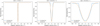 |
Fig. 3 Simulated CCF (solid blue line) and Gaussian fitting (dashed orange line). Left: input value veq sin i★ = 1 km s−1. Center: input value veq sin i★ = 10 km s−1. Right: input value veq sin i★ = 50 km s−1. |
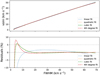 |
Fig. 4 Correlation between the Gaussian fit’s FWHM and the input veq sin i★ of the synthetic line profiles in the whole 0–50 km s−1 weq sin i★ (0–70 km s−1 FWHM) range. Upper panel: correlation between the FWHM and veq (black line) and the relative linear fit (blue dotted line), quadratic fit (orange dotted line), cubic fit (green dashed line), and fourth degree polynomial fit (red dashed line). Lower panel: residuals of the fits. The horizontal grey lines outline the 5% difference between the fit and the data. |
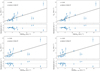 |
Fig. 6 Linear correlations (black solid lines) between the four data sets derived from the FWHMDRS computed by the HARPS-N DRS with the G2 mask (x-axis) and the stellar equatorial velocity veq (y-axis) for our set of calibrators. The Spearman’s correlation coefficient r and p-value are shown in the plots. Upper left: linear correlation between FWHMDRS and veq and relative residuals. Upper right: linear correlation between FWHMmic and veq and relative residuals. Lower left: linear correlation between FWHMmac and veq and relative residuals. Lower right: linear correlation between FWHMmic+mac and veq and relative residuals. |
Fit parameters a and b, uncertainties σa and ab, and correlation factor ρ(a, b) for all the relevant equations obtained in this paper.
4 Projected rotational velocity of exoplanet-host stars
We decided to apply our relation to all the HARPS-N observed exoplanet-host stars found in the TNG archive. First, we queried the NASA exoplanet archive again to obtain a complete list of all known exoplanet-host stars with a declination > −25 deg, without any other constraints. We obtained a preliminary list of 3750 exoplanets (2753 host stars).
We queried the TNG archive3 with a self-written python code using the pyvo module4 in an asynchronous Table Access Protocol (TAP) query, retrieving up to ten public CCF FITS files for each target. We found data for 313 stars, but some of them are useless for different reasons, for example fast rotating stars, a signal-to-noise ratio (S/N) that is too low, and M-type stars having been reduced with the M2 mask.
We point out here that the CCFs of M-type stars may be used if they are computed with the K5 mask: this results in a noisier, but more physically significant CCF. We were also able to recover the M-type stars reduced with the M2 mask that were observed within the GAPS program: in this case, we could once again reduce the spectra with the K5 mask using the YABI platform (Hunter et al. 2012) hosted at the IA2 Data Center5.
In the end, we had to discard some non-GAPS stars with only M2-mask public CCFs, and others stars whose CCFs had a S/N that was too low, or the wrong input radial velocity. We estimated the veq sin i★ for all the 273 remaining targets with FWHMDRS < 20 km s−1. The full table with our veq sin i★ values is available at CDS, an extract is shown in Table 4; the errors were computed using Eq. (11).
Some of the objects in our sample have both G2 and K5 CCFs in the TNG archive, and so we were able to directly compare the results of the two calibrations, in order to quantify the effect of a spectral-type mismatch on the resulting veq sin i★ (see Fig. 7). These objects have a relatively small range of veq sin i★, but still the results agree with less than a 0.5 km s−1 difference for veq sin i★ < 4 km s−1, and with less than 1 km s−1 for veq sin i★ > 4 km s−1. Still, to ensure the best possible result, care should be taken to reduce every star with the more appropriate mask. Usually this is already done, because the better the star-mask match, the smaller the error is for the radial velocity computed by the DRS, but sometimes the stellar type is unknown prior to the observations and a mismatch may occur. Possible mismatches between hotter stars (early F-type or above) and the G2 mask are not considered here because hotter stars are usually also fast rotators and they would naturally fall outside the applicability range of our relation (FWHMDRS < 20 km s−1). Because we relied on the public data present in the TNG archive, there are a few mismatches between the stellar type and mask in our sample, but in all these cases we have veq sin i★ < 4 km s−1, so the mismatches should not heavily affect the results.
4.1 Comparison with the literature
Out of the stars listed in Table 4, 206 had also veq sin i★ values from the literature, so we could compare our results with them (see Fig. 8). As a sanity check, we used this larger sample to test our relations: we calibrated the G2 and K5 FWHMDRS values using the whole set of literature veq sin i★ values. The resulting relations are as follows:
 (14)
(14)
As it is shown in Fig. 9, there is almost no difference between the relation obtained using the whole literature data set and the original one obtained from the selected calibrators (Table 1) for the G2 mask, while the situation is different when using the K5 mask (see the black solid line and red dashed line in Fig. 10). In this case, the spread is larger (and the Spearman’s r coefficient lower), and so is the difference between the original calibration and the new one. We also lack reliable data points with FWHMDRS > 12 km s−1, and the literature veq Sin i★ values are very spread out. The latter fact could be caused by the type of stars that are usually reduced using the K5 mask, that is mid and late K-type and early M-type stars: these objects may be very active and this could affect both the shape of the CCF (and thus the FWHMDRS) and the veq sin estimation performed in the literature. To better investigate this behaviour, and to check the possible limitations of our relations’ applicability range, we looked at the sample considering also the stellar parameters of the stars, that is Teff, log ɡ, and [Fe/H]. We recovered the parameters from SIMBAD6 (Wenger et al. 2000) using an automated python query. We show the results in Fig. 11 for the G2 relation, and in Fig. 12 for the K5 relation. While there is no obvious trend in looking at the results from the G2 relation, we can see that stars with log ɡ < 3.5 tend to cluster below the one-to-one correlation when comparing the results from the K5 relation to the literature veq sin i★ values. If we perform a linear fit between our veq sin i★ and the literature veq sin i★ only for stars with log ɡ > 3.5 (blue dotted line in Fig. 10), then the resulting relation agrees much better with that obtained from the selected calibrators:
 (15)
(15)
While we advise using Eq. (7) to compute veq sin i★ because we trust our selected calibrators better, in Table 2 we also list the parameters’ errors and correlation factors needed to compute the errors when using Eq. (14) (G2 mask only) and Eq. (15) (K5 mask).
We can assume that, at least in the case of the K5 sample, our relations are applicable only for stars with log ɡ > 3.5, that is mostly main sequence stars, but also some subgiant and red giant stars may fall in the applicability range. Unfortunately, we do not have a wide enough range of log ɡ values in our G2 sample to test the same behaviour (see Fig. 11, middle panel); however, considering that the G2 mask used in the HARPS-N DRS is optimized for the Sun, we can infer that also the G2 relation is best suited for main-sequence stars.
Comparing our results with the literature veq sin i★, we found no stars where our veq sin i★ differs more the 3σ from the literature value, and only four where the difference is larger than 2σ (WASP-1, WASP-127, TYC 1422-614-1, and TYC 3667-1280-1). Taking into account the very different methods used in literature to compute veq sin i★, this is a good indicator of the robustness and reliability of our  relation.
Computed veq sin i★ of exoplanet-host stars.
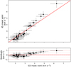 |
Fig. 7 Results obtained with the G2 and the K5 relations for a subset of stars where both CCFs are available. Upper panel: comparison between veq sin i★ obtained with the G2 relation (x-axis) and the K5 relation (y/-axis). The red line shows the one-to-one correlation. Lower panel: residuals. |
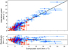 |
Fig. 8 Comparison between veq sin values from the literature (y-axis) and estimated from the CCF FWHMDRS (x-axis). Upper panel: blue dots are values computed with the G2 mask relation, and red triangles are those computed with the K5 mask relation. The black line shows the one-to-one correlation. Lower panel: residuals of the one-to-one correlation shown above. |
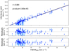 |
Fig. 9 Comparison between the G2 FWHMDRS and the literature veq sin i★ values. Upper panel: correlation between the G2 FWHMDRS (x-axis) and the literature veq sin i★ values (y-axis), with the Spearman’s correlation coefficient r and p-value shown in the plot. The black line shows the linear fit of the data, and the blue dashed line shows the relation obtained from our selected calibrators (Eq. (7)). Middle panel: residuals of the linear fitting. Lower panel: residuals of the relation from selected calibrators. |
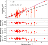 |
Fig. 10 Comparison between the K5 FWHMDRS and the literature veq sin i★ values. Upper panel: correlation between the K5 FWHMDRS (x-axis) and the literature veq sin i★values (y-axis), with the Spearman’s correlation coefficient r and p-value shown in the plot. The black line shows the linear fit of the data, the red dashed line shows the relation obtained from our selected calibrators (Eq. (7)), and the blue dotted line shows the linear fit after removing the stars with log ɡ < 3.5. Lower panels: residuals of the linear fitting, the relation from selected calibrators, and the linear fitting after removing the stars with log ɡ < 3.5. |
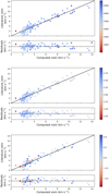 |
Fig. 11 Comparison between our veq sin i★ (x-axis) and the literature values (y-axis) when using the G2 relation, colour-coded according to the stellar parameters Teff (upper panel), log ɡ (middle panel), and [Fe/H] (lower panel). |
4.2 Stellar inclination
We focussed on the results we obtained for stars with no veq sin literature value to see if we were able to recover an estimate of the stellar inclination i★. We did not perform this work on the other targets because our results do not differ much from those already in the literature, and so we do not expect any substantial changes or improvements on i★.
We used Eq. (1) to compute i★, which means that we could only work with objects with known Prot and R★. In some cases, the exoplanetary orbit inclination was known: we could then compare it to i★ so as to check the spin-orbit alignment of the system. Because of the sometimes large errors on the various parameters, many i★ results were compatible with the whole range of possible inclinations.
We show in Table 5 only the results that set some constrains on the stellar possible inclination. While in most cases our results are compatible with aligned, edge-on planetary systems, we still found one system that shows a difference between i★ and ip around the 2σ level (K2-173), and another (HD 13931) where the i★ and ip values point to a possibly aligned, but not edge-on system.
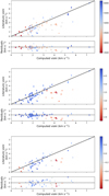 |
Fig. 12 Comparison between our veq sin i★ (x-axis) and the literature values (y-axis) when using the K5 relation, colour-coded according to the stellar parameters Teff (upper panel), log ɡ (middle panel), and [Fe/H] (lower panel). |
5 Extension to other spectrographs
The relations found in our work between FWHMDRS and veq sin i★ are optimized for a specific combination of instruments, software, and stellar masks. While there are other spectrographs with dedicated DRS, and a few of them also deliver the spectra’s CCFs as output, the different resolution, instrumental effects, wavelength ranges, numerical codes used to compute the CCF, and stellar masks could heavily influence the FWHMDRS-veq sin i★ relation. A possible exception could be the HARPS spectrograph (Mayor et al. 2003), of which HARPS-N is a twin, not only concerning the hardware, but also the software, as HARPS and HARPS-N have almost the same DRS.
To test this assumption, we checked the public archives of two spectrographs with a similar spectral range as HARPS-N: HARPS (which also has the same resolution, telescope aperture, and DRS as HARPS-N) and SOPHIE7. Both spectrographs have been used for many years in the exoplanets’ search and characterization field, guaranteeing the availability of a large amount of public data of exoplanet-host stars. The main characteristics of HARPS-N, HARPS, and SOPHIE are listed in Table 6. SOPHIE has a HR and a high-efficiency (HE) mode, but for a more direct comparison with HARPS-N we focus sed on the HR mode spectra to start. Both HARPS and SOPHIE have dedicated DRS that deliver the spectra’s CCFs and their FWHMs using stellar masks similar (or, in the case of HARPS, identical) to the HARPS-N ones. We note here that also SOPHIE DRS is adapted from the HARPS DRS, so the three instruments have the same or a very similar DRS.
We searched the dedicated HARPS8 and SOPHIE9 archives for objects listed in Table 4 to download their HARPS and SOPHIE CCFs. We selected only the CCFs obtained with either the G2 or K5 mask in HR mode, up to a maximum of 50 per object, so that, when possible, we could recover a statistically robust median FWHMDRS for each object. We then computed the veq sin i★ from the median FWHMDRS using Eq. (7), and we compared the results with our HARPS-N veq sin i★. Figure 13 shows the comparison between the HARPS-N and HARPS results, and Fig. 14 shows the comparison between the HARPS-N and SOPHIE results.
It is plainly visible that the twin status of the HARPS and HARPS-N spectrographs would allow us to use the HARPS-N calibration directly with the HARPS data. It is interesting to note that because we used HARPS spectra observed both before and after 2015, this is true for HARPS data taken both before and after the change of fibres (Lo Curto et al. 2015), even if this change should have slightly affected the FWHMDRS.
The situation regarding the SOPHIE data is slightly different: applying the HARPS-N relation to the SOPHIE data results in veq sin i★ values consistently overestimated, in particular at the lower end of the range. This is not surprising since the lower resolution of SOPHIE as compared to HARPS-N result in larger FWHMDRS values due to the greater instrumental broadening. Still, the effect is not simply a rigid shift, but it appears as a parabolic trend. We manipulated the SOPHIE FWHMDRS values in order to correct them for the different instrumental resolution, using the following equation:
 (16)
(16)
where c is the speed of light in km s−1, and RSOPHIE and RHARPS–N are the resolution of SOPHIE and HARPS-N, respectively (see Table 6). The veq sin i★ values computed with FWHMnew are in much better agreement with those derived from HARPS-N data, as shown in Fig. 15. While the spread between HARPS-N and SOPHIE veq sin i★ values is a bit larger than that between the HARPS-N and HARPS ones, it still seems that our relation could also be used with the SOPHIE data, once they are corrected for the difference in resolution.
To better test this assumption, we also selected the SOPHIE CCFs computed from the spectra observed in the HE mode and then we compared the veq sin i★ computed from both the FWHMDRS and FWHMnew. The FWHMnew values were derived using Eq. (16) with the HE resolution. The results are shown in Fig. 16: while correcting for the resolution does improve the agreement between HARPS-N and SOPHIE HE veq sin i★ values, the results are still discrepant. It seems then that a simple correction for the different resolutions is not enough to adapt our relation to a different spectrograph, at least when the resolution difference is large enough. This assumes that there are not any other factors at play, such as a difference in the code to compute HR and HE CCFs in the SOPHIE DRS.
Unfortunately, we cannot test our method further on any other instrument because very few spectrographs are equipped with dedicated DRS that also yield the CCFs in addition to the reduced spectra. ESPRESSO has the same capabilities (and a DRS derived from the HARPS one), but there are not enough public data from this instrument for a meaningful comparison. We were unable to compare the HARPS-N results with those obtained with instruments with a very different spectral coverage (such as the visible and near-infrared spectrograph CARMENES or the near-infrared spectrograph GIANO-B), because their DRSs do not compute any CCFs.
Still, in case any other future DRS will also yield the CCFs, it will be of fundamental importance to calibrate or check and adapt this relation for each combination of instruments, wavelength range, spectral resolution, mathematical recipe (to compute both the CCF and FWHM), and stellar mask. While the work is quite straightforward in the case of instruments such as HARPS-N (which offers a single, fixed choice of wavelength coverage and resolution), it may become slightly more complex when applied to instruments such as ESPRESSO (with three different resolving powers) or UVES (where a wide range of choices in both wavelength coverage and spectral resolution is available). In any case, the strategy detailed in this paper in order to calibrate a  relation may be applied to any other relevant cases including self-made codes, allowing for the information carried in the CCFs to be better exploited.
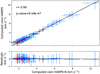 |
Fig. 13 Comparison between veq sin i★ computed from the HARPS-N FWHMDRS (x-axis) and those computed from the HARPS FWHMDRS (y-axis). Upper panel: the blue dots are the values computed with the G2 mask relation, and the red triangles are those computed with the K5 mask relation. The black line shows the one-to-one correlation. Lower panel: residuals. |
Stellar inclination i★ derived from our veq sin i★ values, compared with the planetary orbit inclination ip, if known.
Main characteristics of the HARPS-N, HARPS, and SOPHIE spectrographs.
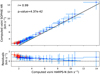 |
Fig. 14 Comparison between veq sin i★ computed from the HARPS-N FWHMDRS (x-axis) and those computed from the SOPHIE HR FWHMDRS (y-axis). Upper panel: the blue dots are the values computed with the G2 mask relation, and the red triangles are those computed with the K5 mask relation. The black line shows the one-to-one correlation. Lower panel: residuals. |
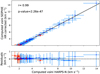 |
Fig. 15 Comparison between veq sin i★ computed from the HARPS-N FWHMDRS (x-axis) and those computed from the corrected SOPHIE HR FWHMnew (y-axis). Upper panel: the blue dots are the values computed with the G2 mask relation, and the red triangles are those computed with the K5 mask relation. The black line shows the one-to-one correlation. Lower panel: residuals. |
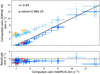 |
Fig. 16 Comparison between veq sin i★ computed from the HARPS-N FWHMDRS (x-axis) and those computed with SOPHIE in HE mode (y-axis). Upper panel: orange triangles and light blue dots are the results from SOPHIE HE FWHMDRS with the K5 and G2 relation, respectively, while the red triangles and blue dots are the results from the corrected SOPHIE HE FWHMnew (y-axis). The black line shows the one-to-one correlation. Lower panel: residuals for the corrected SOPHIE HE FWHMnew only. |
6 Conclusions
Using a well-defined set of calibrators, we were able to obtain two straightforward relations to obtain an estimation of the stellar veq sin i★ directly from the FWHMDRS computed by the HARPS-N DRS using the G2 and K5 masks (see Eq. (7)). These calibrations may be applied when the FWHMDRS value is less than 20 km s−1. For larger values, other methods to compute the veq sin i★ are more accurate (i.e. Fourier transform or rotational profile fitting). Other relations were computed to be used when it is possible to estimate vmicro and/or vmacro, and thus remove their contribution to the FWHMDRS.
We applied our basic relations to all the exoplanet-host stars found in the HARPS-N public archive and in the GAPS private data with CCFs computed with the G2 or K5 mask and FWHMDRS < 20 km s−1: we obtained a catalogue of homogeneous veq sin i★ measurements for 273 exoplanet-host stars. Of these stars, 206 have literature values of veq sin i★: comparing our results with those, we found a very good agreement, with no object differing more than 3σ. Considering the stellar parameters when comparing our results with the literature, we constrained our relation to stars with log ɡ > 3.5.
We can reliably affirm that our simple  relations give solid results, comparable with those obtained with more sophisticated methods such as spectral synthesis. While our errors may overall be larger than those obtained in the literature, our results would still be useful in characterizing exo-planetary properties, and they may be used as a starting point for a more detailed analysis of the exoplanetary systems. In fact, we were able to determine or constrain the stellar inclination for 12 exoplanet-host stars with no previous veq sin i★ measurements, finding hints of spin-orbit misalignment in the K2-173 system.
We also tested our relations on the FWHMDRS computed by the HARPS and SOPHIE DRS, and we conclude that Eq. (7) may be used as it is also with HARPS data taken in high accuracy mode (R = 115 000). It would be possible to use our relation on the SOPHIE HR data once they are corrected for the different resolution, while using the SOPHIE HE data would require some additional fine-tuning. Still, the strategy detailed in this paper (selection of the calibration, creation of the FWHMDRS-veq sin i★ relation, test of the applicability range) may be used to calibrate other  , with different combinations of instrument resolutions, wavelength ranges, mathematical codes (to compute both the CCF and FWHM), and stellar masks.
Acknowledgements
This paper is based on observations collected with the 3.58 m Telescopio Nazionale Galileo (TNG), operated on the island of La Palma (Spain) by the Fundación Galileo Galilei of the INAF (Istituto Nazionale di Astrofísica) at the Spanish Observatorio del Roque de los Muchachos, in the frame of the programme Global Architecture of Planetary Systems (GAPS). This research used the facilities of the Italian Center for Astronomical Archive (IA2) operated by INAF at the Astronomical Observatory of Trieste. This research has made use of the SIMBAD database, operated at CDS, Strasbourg, France L. M. acknowledges support from the “Fondi di Ricerca Scientifica dAteneo 2021” of the University of Rome “Tor Vergata”. G.S. acknowledges support from CHEOPS ASI-INAF agreement n. 2019-29-HH.0.
References
- Adibekyan, V. Z., Delgado Mena, E., Sousa, S. G., et al. 2012, A&A, 547, A36 [NASA ADS] [CrossRef] [EDP Sciences] [Google Scholar]
- Anderson, D. R., Collier Cameron, A., Delrez, L., et al. 2014, MNRAS, 445, 1114 [NASA ADS] [CrossRef] [Google Scholar]
- Bakos, G. Á., Hartman, J., Torres, G., et al. 2011, ApJ, 742, 116 [NASA ADS] [CrossRef] [Google Scholar]
- Baranne, A., Queloz, D., Mayor, M., et al. 1996, A&AS, 119, 373 [NASA ADS] [CrossRef] [EDP Sciences] [Google Scholar]
- Benomar, O., Masuda, K., Shibahashi, H., & Suto, Y. 2014, PASJ, 66, 94 [NASA ADS] [Google Scholar]
- Berger, T. A., Huber, D., Gaidos, E., & van Saders, J. L. 2018, ApJ, 866, 99 [NASA ADS] [CrossRef] [Google Scholar]
- Biazzo, K., D’Orazi, V., Desidera, S., et al. 2022, A&A, 664, A161 [NASA ADS] [CrossRef] [EDP Sciences] [Google Scholar]
- Bonomo, A. S., Desidera, S., Benatti, S., et al. 2017, A&A, 602, A107 [NASA ADS] [CrossRef] [EDP Sciences] [Google Scholar]
- Boyajian, T., von Braun, K., Feiden, G. A., et al. 2014, MNRAS, 447, 846 [Google Scholar]
- Brewer, J. M., Fischer, D. A., Valenti, J. A., & Piskunov, N. 2016, ApJS, 225, 41 [Google Scholar]
- Buchhave, L. A., Bakos, G. Á., Hartman, J. D., et al. 2010, ApJ, 720, 1118 [NASA ADS] [CrossRef] [Google Scholar]
- Butler, R. P., Marcy, G. W., Williams, E., Hauser, H., & Shirts, P. 1997, ApJ, 474, L115 [Google Scholar]
- Butters, O. W., West, R. G., Anderson, D. R., et al. 2010, A&A, 520, L10 [NASA ADS] [CrossRef] [EDP Sciences] [Google Scholar]
- Choi, J., Dotter, A., Conroy, C., et al. 2016, ApJ, 823, 102 [Google Scholar]
- Collins, K. A., Kielkopf, J. F., & Stassun, K. G. 2017, AJ, 153, 78 [NASA ADS] [CrossRef] [Google Scholar]
- Cosentino, R., Lovis, C., Pepe, F., et al. 2014, Proc. SPIE, 9147, 91478C [Google Scholar]
- Covino, E., Esposito, M., Barbieri, M., et al. 2013, A&A, 554, A28 [NASA ADS] [CrossRef] [EDP Sciences] [Google Scholar]
- Crossfield, I. J. M., Petigura, E., Schlieder, J. E., et al. 2015, ApJ, 804, 10 [NASA ADS] [CrossRef] [Google Scholar]
- Crouzet, N., McCullough, P. R., Burke, C., & Long, D. 2012, ApJ, 761, 7 [CrossRef] [Google Scholar]
- Dalba, P. A., Kane, S. R., Isaacson, H., et al. 2021, AJ, 161, 103 [NASA ADS] [CrossRef] [Google Scholar]
- Díaz, M. R., Jenkins, J. S., Tuomi, M., et al. 2018, AJ, 155, 126 [CrossRef] [Google Scholar]
- Díez Alonso, E., Suárez Gómez, S. L., González Hernández, J. I., et al. 2018, MNRAS, 476, L50 [CrossRef] [Google Scholar]
- Dotter, A. 2016, ApJS, 222, 8 [Google Scholar]
- Doyle, A. P., Davies, G. R., Smalley, B., Chaplin, W. J., & Elsworth, Y. 2014, MNRAS, 444, 3592 [Google Scholar]
- Eastman, J. D., Rodriguez, J. E., Agol, E., et al. 2019, ArXiv e-prints [arXiv:1907.09480] [Google Scholar]
- Esposito, M., Covino, E., Desidera, S., et al. 2017, A&A, 601, A53 [NASA ADS] [CrossRef] [EDP Sciences] [Google Scholar]
- Fischer, D. A., Vogt, S. S., Marcy, G. W., et al. 2007, ApJ, 669, 1336 [NASA ADS] [CrossRef] [Google Scholar]
- Gaia Collaboration (Prusti, T., et al.) 2016, A&A, 595, A1 [NASA ADS] [CrossRef] [EDP Sciences] [Google Scholar]
- Gaia Collaboration (Brown, A. G. A., et al.) 2021, A&A, 649, A1 [NASA ADS] [CrossRef] [EDP Sciences] [Google Scholar]
- Gray, D. F. 2008, The Observation and Analysis of Stellar Photospheres (Cambridge: Cambridge University Press) [Google Scholar]
- Hedges, C., Saunders, N., Barentsen, G., et al. 2019, ApJ, 880, L5 [NASA ADS] [CrossRef] [Google Scholar]
- Hellier, C., Anderson, D. R., Collier Cameron, A., et al. 2011, A&A, 535, L7 [NASA ADS] [CrossRef] [EDP Sciences] [Google Scholar]
- Hirano, T., Sanchis-Ojeda, R., Takeda, Y., et al. 2014, ApJ, 783, 9 [CrossRef] [Google Scholar]
- Horne, J. H., & Baliunas, S. L. 1986, ApJ, 302, 757 [Google Scholar]
- Howard, A. W., Johnson, J. A., Marcy, G. W., et al. 2010, ApJ, 721, 1467 [Google Scholar]
- Hunter, A. A., Macgregor, A. B., Szabo, T. O., et al. 2012, Source Code Biol. Med., 7, 1 [CrossRef] [Google Scholar]
- Johnson, J. A., Payne, M., Howard, A. W., et al. 2011, AJ, 141, 16 [Google Scholar]
- Kosiarek, M. R., Crossfield, I. J. M., Hardegree-Ullman, K. K., et al. 2019, AJ, 157, 97 [NASA ADS] [CrossRef] [Google Scholar]
- Küker, M., Rüdiger, G., Olah, K., & Strassmeier, K. G. 2019, A&A, 622, A40 [NASA ADS] [CrossRef] [EDP Sciences] [Google Scholar]
- Lamm, M. H., Bailer-Jones, C. A. L., Mundt, R., Herbst, W., & Scholz, A. 2004, A&A, 417, 557 [NASA ADS] [CrossRef] [EDP Sciences] [Google Scholar]
- Livingston, J. H., Crossfield, I. J. M., Petigura, E. A., et al. 2018, AJ, 156, 277 [NASA ADS] [CrossRef] [Google Scholar]
- Lo Curto, G., Pepe, F., Avila, G., et al. 2015, The Messenger, 162, 9 [NASA ADS] [Google Scholar]
- Ma, B., Ge, J., Muterspaugh, M., et al. 2018, MNRAS, 480, 2411 [Google Scholar]
- Mancini, L., Southworth, J., Ciceri, S., et al. 2014, MNRAS, 443, 2391 [Google Scholar]
- Mancini, L., Esposito, M., Covino, E., et al. 2018, A&A, 613, A41 [NASA ADS] [CrossRef] [EDP Sciences] [Google Scholar]
- Mann, A. W., Johnson, M. C., Vanderburg, A., et al. 2020, AJ, 160, 179 [Google Scholar]
- Mayo, A. W., Vanderburg, A., Latham, D. W., et al. 2018, AJ, 155, 136 [Google Scholar]
- Mayor, M., & Queloz, D. 1995, Nature, 378, 355 [Google Scholar]
- Mayor, M., Pepe, F., Queloz, D., et al. 2003, The Messenger, 114, 20 [NASA ADS] [Google Scholar]
- Mazeh, T., Perets, H. B., McQuillan, A., & Goldstein, E. S. 2015, ApJ, 801, 3 [Google Scholar]
- McLaughlin, D. B. 1924, ApJ, 60, 22 [Google Scholar]
- McQuillan, A., Mazeh, T., & Aigrain, S. 2013, ApJ, 775, L11 [Google Scholar]
- Ment, K., Fischer, D. A., Bakos, G., Howard, A. W., & Isaacson, H. 2018, AJ, 156, 213 [NASA ADS] [CrossRef] [Google Scholar]
- Močnik, T., Clark, B. J. M., Anderson, D. R., Hellier, C., & Brown, D. J. A. 2016, AJ, 151, 150 [CrossRef] [Google Scholar]
- Močnik, T., Southworth, J., & Hellier, C. 2017, MNRAS, 471, 394 [Google Scholar]
- Nikolov, N., Sing, D. K., Pont, F., et al. 2014, MNRAS, 437, 46 [NASA ADS] [CrossRef] [Google Scholar]
- Nordström, B., Mayor, M., Andersen, J., et al. 2004, A&A, 418, 989 [Google Scholar]
- Nutzman, P., Gilliland, R. L., McCullough, P. R., et al. 2010, ApJ, 726, 3 [Google Scholar]
- Pepe, F., Mayor, M., Galland, F., et al. 2002, A&A, 388, 632 [NASA ADS] [CrossRef] [EDP Sciences] [Google Scholar]
- Philipot, F., Lagrange, A. M., Rubini, P., Kiefer, F., & Chomez, A. 2023, A&A, 670, A65 [NASA ADS] [CrossRef] [EDP Sciences] [Google Scholar]
- Queloz, D., Eggenberger, A., Mayor, M., et al. 2000, A&A, 359, L13 [NASA ADS] [Google Scholar]
- Rainer, M., Borsa, F., & Affer, L. 2020, Exp. Astron., 49, 73 [Google Scholar]
- Reinhold, T., & Hekker, S. 2020, A&A, 635, A43 [NASA ADS] [CrossRef] [EDP Sciences] [Google Scholar]
- Ricker, G. R., Winn, J. N., Vanderspek, R., et al. 2015, J. Astron. Teles. Instrum. Syst., 1, 014003 [Google Scholar]
- Roberts, D. H., Lehar, J., & Dreher, J. W. 1987, AJ, 93, 968 [Google Scholar]
- Rossiter, R. A. 1924, ApJ, 60, 15 [Google Scholar]
- Sada, P. V., & Ramón-Fox, F. G. 2016, PASP, 128, 024402 [NASA ADS] [CrossRef] [Google Scholar]
- Santerne, A., Hébrard, G., Lillo-Box, J., et al. 2016, ApJ, 824, 55 [CrossRef] [Google Scholar]
- Southworth, J. 2011, MNRAS, 417, 2166 [Google Scholar]
- Southworth, J. 2012, MNRAS, 426, 1291 [NASA ADS] [CrossRef] [Google Scholar]
- Stassun, K. G., Collins, K. A., & Gaudi, B. S. 2017, AJ, 153, 136 [Google Scholar]
- Stassun, K. G., Oelkers, R. J., Paegert, M., et al. 2019, AJ, 158, 138 [Google Scholar]
- Stumpe, M. C., Smith, J. C., Van Cleve, J. E., et al. 2012, PASP, 124, 985 [Google Scholar]
- Villaver, E., Niedzielski, A., WolszCzan, A., et al. 2017, A&A, 606, A38 [NASA ADS] [CrossRef] [EDP Sciences] [Google Scholar]
- Wenger, M., OChsenbein, F., Egret, D., et al. 2000, A&AS, 143, 9 [NASA ADS] [CrossRef] [EDP Sciences] [Google Scholar]
- Winn, J. N., Noyes, R. W., Holman, M. J., et al. 2005, ApJ, 631, 1215 [Google Scholar]
- Zechmeister, M., & Kürster, M. 2009, A&A, 496, 577 [CrossRef] [EDP Sciences] [Google Scholar]
All Tables
Fit parameters a and b, uncertainties σa and ab, and correlation factor ρ(a, b) for all the relevant equations obtained in this paper.
Stellar inclination i★ derived from our veq sin i★ values, compared with the planetary orbit inclination ip, if known.
All Figures
|
Fig. 1 Comparison in the Teff-R★ parameter space between the sample of stars analysed in this work (red circles) and the currently known exoplanet-host stars (grey dots) as retrieved from the NASA Exoplanet Catalog. |
| In the text | |
|
Fig. 2 Comparison of the stellar radii and effective temperatures obtained via the SED fitting described in Sect. 2 with literature values. Upper panels: correlations’ plot between our values and the literature ones for R★ (left panel) and Teff (right panel). Lower panels: residual plots showing the difference between our values and the literature ones. |
| In the text | |
|
Fig. 3 Simulated CCF (solid blue line) and Gaussian fitting (dashed orange line). Left: input value veq sin i★ = 1 km s−1. Center: input value veq sin i★ = 10 km s−1. Right: input value veq sin i★ = 50 km s−1. |
| In the text | |
|
Fig. 4 Correlation between the Gaussian fit’s FWHM and the input veq sin i★ of the synthetic line profiles in the whole 0–50 km s−1 weq sin i★ (0–70 km s−1 FWHM) range. Upper panel: correlation between the FWHM and veq (black line) and the relative linear fit (blue dotted line), quadratic fit (orange dotted line), cubic fit (green dashed line), and fourth degree polynomial fit (red dashed line). Lower panel: residuals of the fits. The horizontal grey lines outline the 5% difference between the fit and the data. |
| In the text | |
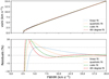 |
Fig. 5 Same as Fig. 4, but limited to the 0–20 km s−1 FWHM range. |
| In the text | |
|
Fig. 6 Linear correlations (black solid lines) between the four data sets derived from the FWHMDRS computed by the HARPS-N DRS with the G2 mask (x-axis) and the stellar equatorial velocity veq (y-axis) for our set of calibrators. The Spearman’s correlation coefficient r and p-value are shown in the plots. Upper left: linear correlation between FWHMDRS and veq and relative residuals. Upper right: linear correlation between FWHMmic and veq and relative residuals. Lower left: linear correlation between FWHMmac and veq and relative residuals. Lower right: linear correlation between FWHMmic+mac and veq and relative residuals. |
| In the text | |
|
Fig. 7 Results obtained with the G2 and the K5 relations for a subset of stars where both CCFs are available. Upper panel: comparison between veq sin i★ obtained with the G2 relation (x-axis) and the K5 relation (y/-axis). The red line shows the one-to-one correlation. Lower panel: residuals. |
| In the text | |
|
Fig. 8 Comparison between veq sin values from the literature (y-axis) and estimated from the CCF FWHMDRS (x-axis). Upper panel: blue dots are values computed with the G2 mask relation, and red triangles are those computed with the K5 mask relation. The black line shows the one-to-one correlation. Lower panel: residuals of the one-to-one correlation shown above. |
| In the text | |
|
Fig. 9 Comparison between the G2 FWHMDRS and the literature veq sin i★ values. Upper panel: correlation between the G2 FWHMDRS (x-axis) and the literature veq sin i★ values (y-axis), with the Spearman’s correlation coefficient r and p-value shown in the plot. The black line shows the linear fit of the data, and the blue dashed line shows the relation obtained from our selected calibrators (Eq. (7)). Middle panel: residuals of the linear fitting. Lower panel: residuals of the relation from selected calibrators. |
| In the text | |
|
Fig. 10 Comparison between the K5 FWHMDRS and the literature veq sin i★ values. Upper panel: correlation between the K5 FWHMDRS (x-axis) and the literature veq sin i★values (y-axis), with the Spearman’s correlation coefficient r and p-value shown in the plot. The black line shows the linear fit of the data, the red dashed line shows the relation obtained from our selected calibrators (Eq. (7)), and the blue dotted line shows the linear fit after removing the stars with log ɡ < 3.5. Lower panels: residuals of the linear fitting, the relation from selected calibrators, and the linear fitting after removing the stars with log ɡ < 3.5. |
| In the text | |
|
Fig. 11 Comparison between our veq sin i★ (x-axis) and the literature values (y-axis) when using the G2 relation, colour-coded according to the stellar parameters Teff (upper panel), log ɡ (middle panel), and [Fe/H] (lower panel). |
| In the text | |
|
Fig. 12 Comparison between our veq sin i★ (x-axis) and the literature values (y-axis) when using the K5 relation, colour-coded according to the stellar parameters Teff (upper panel), log ɡ (middle panel), and [Fe/H] (lower panel). |
| In the text | |
|
Fig. 13 Comparison between veq sin i★ computed from the HARPS-N FWHMDRS (x-axis) and those computed from the HARPS FWHMDRS (y-axis). Upper panel: the blue dots are the values computed with the G2 mask relation, and the red triangles are those computed with the K5 mask relation. The black line shows the one-to-one correlation. Lower panel: residuals. |
| In the text | |
|
Fig. 14 Comparison between veq sin i★ computed from the HARPS-N FWHMDRS (x-axis) and those computed from the SOPHIE HR FWHMDRS (y-axis). Upper panel: the blue dots are the values computed with the G2 mask relation, and the red triangles are those computed with the K5 mask relation. The black line shows the one-to-one correlation. Lower panel: residuals. |
| In the text | |
|
Fig. 15 Comparison between veq sin i★ computed from the HARPS-N FWHMDRS (x-axis) and those computed from the corrected SOPHIE HR FWHMnew (y-axis). Upper panel: the blue dots are the values computed with the G2 mask relation, and the red triangles are those computed with the K5 mask relation. The black line shows the one-to-one correlation. Lower panel: residuals. |
| In the text | |
|
Fig. 16 Comparison between veq sin i★ computed from the HARPS-N FWHMDRS (x-axis) and those computed with SOPHIE in HE mode (y-axis). Upper panel: orange triangles and light blue dots are the results from SOPHIE HE FWHMDRS with the K5 and G2 relation, respectively, while the red triangles and blue dots are the results from the corrected SOPHIE HE FWHMnew (y-axis). The black line shows the one-to-one correlation. Lower panel: residuals for the corrected SOPHIE HE FWHMnew only. |
| In the text | |
Current usage metrics show cumulative count of Article Views (full-text article views including HTML views, PDF and ePub downloads, according to the available data) and Abstracts Views on Vision4Press platform.
Data correspond to usage on the plateform after 2015. The current usage metrics is available 48-96 hours after online publication and is updated daily on week days.
Initial download of the metrics may take a while.