| Issue |
A&A
Volume 674, June 2023
|
|
|---|---|---|
| Article Number | A77 | |
| Number of page(s) | 18 | |
| Section | Extragalactic astronomy | |
| DOI | https://doi.org/10.1051/0004-6361/202245548 | |
| Published online | 02 June 2023 | |
Origin of the diffuse 4–8 keV emission in M 82
1
Institut de Ciències del Cosmos (ICCUB), Universitat de Barcelona (IEEC-UB), Martí i Franquès, 1, 08028 Barcelona, Spain
e-mail: This email address is being protected from spambots. You need JavaScript enabled to view it.
2
ICREA, Pg. Lluís Companys 23, 08010 Barcelona, Spain
3
Department of Physics and Astronomy, Johns Hopkins University, Baltimore, MD 21218, USA
4
Space Telescope Science Institute, 3700 San Martin Drive, Baltimore, MD 21218, USA
5
INAF – Osservatorio di Astrofisica e Scienza dello Spazio di Bologna, Via P. Gobetti 93/3, 40129 Bologna, Italy
6
School of Physics and Astronomy, University of Southampton, Highfield, Southampton SO17 1BJ, UK
7
Instituto de Astrofísica de Andalucía (CSIC), Glorieta de la Astronomía s/n, 18008 Granada, Spain
8
Facultad de Ciencias, Universidad de Zaragoza, Pedro Cerbuna 12, 50009 Zaragoza, Spain
9
School of Sciences, European University Cyprus, Diogenes Street, Engomi, 1516 Nicosia, Cyprus
Received:
24
November
2022
Accepted:
10
March
2023
Abstract
We present the first spatially resolved, X-ray spectroscopic study of the 4−8 keV diffuse emission found in the central part of the nearby starburst galaxy M 82 on a few arcsecond scales. The new details that we see allow a number of important conclusions to be drawn on the nature of the hot gas and its origin as well as feedback on the interstellar medium. We use archival data from the Chandra X-ray Observatory with an exposure time of 570 ks. The Fe XXV emission at 6.7 keV, expected from metal-enriched hot gas, is enhanced only in a limited area close to the starburst disc and is weak or almost absent over the rest of the diffuse emission, resulting in spatial variations in equivalent width from < 0.1 keV to 1.9 keV. This shows the presence of non-thermal emission due to inverse Compton scattering of the far-infrared photons by radio emitting cosmic ray electrons. The morphological resemblance between the diffuse X-ray, radio, and far-infrared emission maps support this concept. Our decomposition of the diffuse emission spectrum indicates that ∼70% of the 4−8 keV luminosity originates from the inverse Compton emission. The metal-rich hot gas with a temperature of ≃5 keV makes a minor contribution to the 4−8 keV continuum, but it accounts for the majority of the observed Fe XXV line. This hot gas appears to emerge from the circumnuclear starburst ring and fill the galactic chimneys identified as mid-infrared and radio emission voids. The energetics argument suggests that much of the supernova energy in the starburst site has gone into creating of the chimneys and is transported to the halo. We argue that a hot, rarefied environment produced by strong supernova feedback results in displacing the brightest X-ray and radio supernova remnants which are instead found to reside in giant molecular clouds. We find a faint X-ray source with a radio counterpart, close to the kinematic centre of the galaxy and we carefully examine the possibility that this source is a low-luminosity active galactic nucleus in an advection-dominated accretion flow phase.
Key words: galaxies: starburst / galaxies: individual: M 82 / X-rays: galaxies
© The Authors 2023
 Open Access article, published by EDP Sciences, under the terms of the Creative Commons Attribution License (https://creativecommons.org/licenses/by/4.0), which permits unrestricted use, distribution, and reproduction in any medium, provided the original work is properly cited.
This article is published in open access under the Subscribe to Open model. This email address is being protected from spambots. You need JavaScript enabled to view it. to support open access publication.
1. Introduction
A fundamental ingredient of the superwind model of Chevalier & Clegg (1985) is a hot fluid with a temperature of ∼108 K, created by an injection of kinetic energy mainly from supernovae, and to a lesser degree from stellar winds of massive stars, propagating into a low-density medium in a starburst region. To maintain the kinetic energy for driving a galactic-scale wind, this hot fluid has to be minimally radiative with a long cooling time. The superwind could be observed in hard X-rays above a few keV. The nearby starburst galaxy M 82 shows a large-scale galactic wind at various wavelengths and is an ideal target to examine the wind-driving mechanism. Earlier X-ray imaging of M 82 at the arcsecond resolution with the Chandra X-ray Observatory (Chandra) resolved out bright X-ray binaries which dominate the hard X-ray band and revealed that there is residual diffuse emission surrounding the starburst disc (Griffiths et al. 2000). The spectrum of the diffuse gas exhibits a high-ionisation Fe K line from Fe XXV, characteristic of the thermal emission of a temperature of a few keV, and thus has been identified with the hot fluid as envisaged in the superwind model. Strickland & Heckman (2009) argued that the observed Fe XXV luminosity agrees with the expectation of the Chevalier & Clegg (1985) model. However, if the hard X-ray diffuse emission spectrum is to be explained by thermal emission, the Fe XXV line appears too weak, requiring low Fe metallicity of 0.2−0.3 Z⊙ (Strickland & Heckman 2007; Liu et al. 2014), in contrast with a highly enriched interstellar medium enriched by core-collapse supernovae in starburst galaxies such as M 82. Recent findings of several X-ray supernova remnants (SNRs), which also emit strong Fe XXV but are not resolved in the previous study (Iwasawa 2021), reduce the Fe XXV luminosity originating from the diffuse emission further. A possible explanation is that the continuum of the Fe XXV-emitting gas is much fainter and the majority of the observed continuum emission comes from an extra source such as non-thermal emission (e.g. Strickland & Heckman 2009). Although non-thermal emission due to inverse Compton scattering of far-infrared (FIR) photons by cosmic ray electrons have long been proposed for the hard X-ray emission in M 82 (Hargrave 1974; Schaaf et al. 1989; Moran & Lehnert 1997), the presence of bright X-ray binaries hindered a good measurement of the true diffuse emission properties before Chandra. Even with the Chandra imaging, the inverse Compton emission was disfavoured by Strickland & Heckman (2007) for being too faint. Given the γ-ray detection from M 82 (Abdo et al. 2010) and the importance of cosmic-ray driven winds in starburst galaxies, the starburst-driven non-thermal process warrants a serious consideration.
In this work, we present an updated spatially resolved spectral analysis of the X-ray diffuse emission in the 4−8 keV band using the archival Chandra data. The Fe XXV emission at 6.7 keV is of primary interest, but the cold Fe K emission at 6.4 keV is also present in the diffuse emission spectrum (Strickland & Heckman 2007; Liu et al. 2014). We examine the spatial distributions of these Fe lines and discuss their implications for the origin of the 4−8 keV emission, which seems to support the presence of both the inverse Compton emission and also the metal-rich hot gas.
The distance to M 82 is assumed to be 3.6 Mpc (Freedman et al. 1994). The angular scale is thus 17.4 pc arcsec−1 (1 kpc corresponds to approximately 1 arcmin).
2. Observations
We used the same 13 Chandra ACIS observations of M 82 (Table 1) as in Iwasawa (2021) where details of the observations can be found. These observations were selected from all the Chandra ACIS observations of M 82 for relatively small off axis angles (0.3−2.7 arcsec) for the central starburst region- so that the point spread function (PSF) has small distortion. The major part of this work relating to spectral analysis makes use of the 11 observations with the ACIS-S3, which provide a consistent spectral resolution. The two early AICS-I observations in 1999 were used only for the imaging analysis. The total exposure time of the 11 ACIS-S3 observations is 570 ks and the two ACIS-I observations add an extra 52 ks.
Chandra observations of M 82.
Chandra data reduction and image analysis were carried out by CIAO 4.12 (Fruscione et al. 2006) using the calibration files in CALDB 4.53. Spectral analysis was performed using HEASoft XSPEC (Blackburn et al. 1999; Arnaud 1996).
3. Results
3.1. Image of the 4–8 keV diffuse emission
The 4−8 keV Chandra image integrated over all the 13 observations is shown in Fig. 1. The diffuse emission, as well as a number of discrete sources, is visible. It lies along the starburst disc where the discrete sources are concentrated. Its extension along the major axis (PA ≃ 70°) is ∼700 pc, coinciding with the disc size. The height of the extension above and below the disc is less than 200 pc and the overall shape is elliptical. We adopt an ellipse of semi-major and semi-minor axis lengths of  (=338 pc × 164 pc) with the major axis inclined to PA = 70°, which includes most of the 4−8 keV diffuse emission.
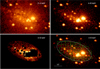 |
Fig. 1. Chandra X-ray images of the central part of M 82 integrated over the 13 observations. Top left: 2−4 keV image. Top right: 4−8 keV band. The colour scale of these two images is in logarithmic with the brightest point sources are saturated. Bottom left: The 4−6 keV image of the ellipse where the data of the diffuse emission spectrum were taken. The detected discrete sources were masked. The region where the brightest ULXs along with a few others are clustered is masked in a block. This image is in a linear scale as the dynamic range of the brightness is narrow: 1−19, as a result of the removal of discrete sources. Bottom right: The same image as top right overlaid by the ellipse and the 38 region segments for spatially resolved spectral study. |
The spectral data were taken from this ellipse, masking the individual discrete sources. We refer to the 21 sources detected within the ellipse in Iwasawa (2021), Xp0 through Xp20. The western part where the bright ultraluminous X-ray sources (ULXs) are clustered was masked in a block so that a sufficiently large area around them is masked to avoid their emission in the PSF wings as well as the bright core emission. This block contains Xp12 through Xp17. These masks for the discrete sources take up 23% of the entire ellipse area of 591 arcsec2. The 4−6 keV continuum image from the ellipse with the masking is also shown in Fig. 1. We note that the 4−6 keV image of the diffuse emission alone has a relatively flat brightness distribution, in the absence of peaky discrete sources, and is shown in a linear scale.
Compared with the 4−8 keV emission, the diffuse emission at lower energies rises sharply towards the disc plane and is more extended, as illustrated by the 2−4 keV image. This soft X-ray extended emission is considered to be the entrained, shocked interstellar medium (ISM), forming part of the large-scale soft X-ray winds. The central part, near the starburst disc in particular, is obscured and subject to suppression by absorption at the lower energies. Even in the 2−4 keV image, the light suppression is visible along the disc. This absorption effect of the order of NH of a few times of 1022 cm−2 practically diminishes above 4 keV and all the discrete sources embedded in the starburst disc are visible in the 4−8 keV image. Likewise, the diffuse emission above 4 keV is largely unaffected by absorption, except for a small part with excess obscuration.
3.2. Total diffuse emission spectrum
3.2.1. Thermal emission lines
Although the soft X-ray emission spectrum is beyond the scope of this work, it is worth illustrating the contrasting characteristics of the emission-line spectrum above and below 4 keV. The broad-band spectrum (Fig. 2) shows strong He-like and H-like K-shell emission from Ne, Mg, Si, S, Ar and Ca in the 1−4 keV range. At energies above 4 keV, the most prominent spectral feature is the Fe K complex in 6−7 keV (Fig. 2), dominated by Fe XXV at ∼6.7 keV. As previously noted by Strickland & Heckman (2007), Liu et al. (2014), a cold Fe K line at 6.4 keV is also present. A line-like excess is detected marginally at 4.5 keV, although the origin is unclear. Since its detection is marginal and is not essential for this work, we leave further details in Appendix B. For all the spectral fits presented below unless stated otherwise, a spectrum was binned so that each bin contains at least one count. A spectral fit was performed on background-corrected data by comparing with a model folded through the detector response, using the C-statistic (Cash 1979).
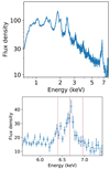 |
Fig. 2. Diffuse emission spectrum of the central part of M 82, obtained from the Chandra ACIS-S. The flux density is in units of 10−14 erg s−1 cm−2 keV−1. Upper panel: The 0.7−8 keV spectrum. Lower panel: The Fe K band spectrum of the same data. The three vertical dotted-lines indicates the expected centroid energies of 6.4 keV, 6.7 keV and 6.96 keV for cold Fe K, Fe XXV and Fe XXVI, respectively. The grey line indicates the fitted model of a power-law and three Gaussian lines. |
We examined temperature and metallicity inferred from the atomic lines of each element by fitting the thermal emission spectrum of apec1 in a narrow energy range, as follows: 1.1−1.7 keV for Mg; 1.5−2.4 keV for Si; 2.1−3 keV for S; 2.7−3.5 keV for Ar; and 3.3−4.3 keV for Ca. With the restricted energy ranges, a temperature and metallicity were inferred by each element independently. A He-like and H-like line ratio mainly drives the temperature determination for Mg, Si, S, for which the emission lines dominate the continuum. This is less true for Ar and Ca, since the slope of strong continuum emission affects the temperature determination. We did not look into the Ne lines, as the energy range of this line also contains substantial emission from the Fe L complex around 1 keV. Cold absorption was fitted. The results are illustrated in Fig. 3. The metallicity remains compatible between the elements at ≃0.6 Z⊙. The gas temperatures inferred from individual elements remain in a limited range of kT ≃ 0.9 − 1.8 keV with a moderately increasing trend as the selected energy range moves higher. The absorption also shows the same increasing trend. Both indicate spectral hardening towards higher energies. This is likely a manifestation of an increasing contribution of a hard continuum component rather than a true rise of temperature or absorption. Therefore we consider that the temperature and NH for Ar and Ca lines, which lie above the strong continuum, are likely similar to those inferred for S emission.
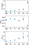 |
Fig. 3. Temperature (kT), metallicity (Z) and absorbing column density (NH) obtained from fitting the apec to the individual line spectra. The NH for the Fe K band spectrum was assumed to be 4 × 1022 cm−2, approximately the middle value obtained for the Ca spectrum, as the energy range of the data is insensitive to NH < 1023 cm−2. |
In contrast, the Fe K line spectrum gives a much higher temperature and a lower metallicity. Fitting to the 6−7.2 keV spectrum gives kT = 4.6 (3.8−5.7) keV and  . In the fit, an additional narrow Gaussian line at 6.4 keV is included. As the energy range is not sensitive to absorption smaller than NH ∼ 1023 cm−2, the central NH value obtained for the Ca K band was assumed but it has no effect on the result. This abrupt change in temperature and metallicity above and below 4 keV, in addition to the morphological difference in image, signals a transition between the two diffuse emission components of different origins taking place at around 4 keV. The increasing kT and NH towards the transition energy suggest spectral hardening which is likely caused by the harder component and/or more absorption. The soft X-ray wind emission therefore lies in the foreground of the harder component exhibiting the Fe K emission.
3.2.2. Fe K complex
The Fe K line complex (Fig. 2) is described here by multiple Gaussians. The dominant Fe XXV is most likely of thermal origin. It is a triplet that is not resolved at the CCD resolution. Fitting a single Gaussian to a simulated apec spectrum gives a centroid energy of 6.68 keV with a slight broadening of σ ∼ 30 eV, when kT is in the range of 4−6 keV (Appendix A), which is inferred from the apec fit to the Fe K band. The observed data show the centroid energy of 6.67 ± 0.01 keV and the width of σ = 58 ± 17 eV, slightly broader than expected. Two other Gaussian lines for a cold Fe K line at 6.4 keV and Fe XXVI at 6.96 keV were added, assuming they are narrow and unresolved. Respective line intensities were fitted and the results are shown in Table 2. The continuum is modelled by a power-law by fitting the 4.1−8 keV data (the lower energy bound at 4.1 keV was chosen to eliminate the Ca emission). The absorbing NH of 4 × 1022 cm−2 and the marginally detected 4.5 keV line are also included. The power-law slope, energy index2, was found to be α = 1.28 ± 0.12.
Fe K line complex of the diffuse emission spectrum.
Notwithstanding the weak detection of Fe XXVI, the Fe XXVI to Fe XXV ratio of 0.14 ± 0.09 indicates a temperature of kT ≈ 4.5 ± 1 keV (Appendix A), in agreement with that inferred from the apec fit. However, the Fe XXV line broadening as observed above may indicate a contribution from a lower temperature emission, as discussed later, and thus the true temperature of the gas may be higher than that inferred from the apparent Fe XXV to Fe XXVI ratio (see further details in Sect. 4).
3.3. Spectral variations across the diffuse emission
3.3.1. Region segments
Here, we investigate spectral variations across the 4−8 keV diffuse emission of M 82. We set 38 rectangular region-segments covering the diffuse emission (Fig. 1) and examined the individual spectra taken there. These region segments were placed by avoiding the discrete sources, except for the two transient sources (the reason for this exception is described below). We label them as dX0 through dX37. The segments dX0 through dX20 are on the northern side of the starburst disc while dX21 through dX33 on the southern side. The two segments, dX34 and dX35, lie within the starburst disc, placed in the small gaps between crowded discrete sources.
The two additional segments, dX36 and dX37, contain transient sources, Xp7 and Xp11 as labelled in Iwasawa (2021), respectively. Since the transient sources were in quiescence, no excess emission is visible at their positions (Appendix C) and we used the data for their quiescent state. As the flaring of Xp7 occurred in the two early ACIS-I observations used only for imaging, the exposure time of the dX36 spectrum remains the same as the spectra of the other segments, integrated over all the 11 ACIS-S observations. As for Xp11, the transient flaring occurred in the three observations in 2010. The spectrum of dX37 was then produced, omitting those observations, and its resulted exposure time is 450 ks, as opposed to the full 570 ks.
The segment sizes were chosen to minimise the dispersion of source counts contained between the individual segments where allowed by the positions of the discrete sources. As a result, the 4−8 keV counts of those segments range between 150 and 400 counts, with the mean of 274 counts and the standard deviation of 72 counts. The broad-band spectra of these 38 region segments are shown in Fig. F.1.
3.3.2. Mapping the spectral variations
Our primary interest is to investigate spatial variations of the Fe K lines. We modelled the 4−8 keV spectrum of each segment with a power-law continuum and two Gaussian lines at 6.4 keV and 6.67 keV. No absorption is included. The Fe lines were assumed to be narrow at those energies and their normalisations were fitted. The continuum flux of each region was estimated in the 4−6 keV band from the fit. The power-law energy index, α, measured for the continuum in the same energy range was also recorded for each region.
Based on the above fits, we constructed surface brightness maps of the 4−6 keV continuum, cold Fe and Fe XXV emission over the 38 region segments, as shown in Fig. 4. The maps of 4−6 keV continuum slope and equivalent width (EW) of the two Fe lines are also shown. The same values given in the maps with the 68% error intervals are plotted in the order of the segment number in Fig. 5. A few spectra with a 4−6 keV slope close to zero indicate that they might be more absorbed than the rest since they have NH of ∼1023 cm−2 (Appendix D).
 |
Fig. 4. Spatial variations of spectral properties over the hard-band diffuse emission. Left: Surface brightness (upper panel) in units of 10−15 erg s−1 cm−2 arcsec−2 and energy index of power-law continuum (lower panel) in the 4−6 keV band. Middle: Surface brightness of 6.67 keV Fe XXV emission in units of 10−9 ph cm−2 s−1 arcsec−2 and line EW in units of keV. Right: Surface brightness and line EW of 6.4 keV cold Fe K emission in the same units as the Fe XXV emission. |
The continuum emission shows high surface brightness near the starburst disc which declines gradually towards larger radii, in agreement with the 4−6 keV count image shown in Fig. 1. With respect to the disc plane, the brightness distribution appears to be similar between the northern and southern sides, when discounting the lowest surface brightness regions on the north-east corner. On the contrary, the Fe XXV emission is markedly stronger on the northern side, particularly evident in its eastern part. Such a north-south asymmetry is not obvious in the cold Fe emission.
The above observation regarding the north-south brightness symmetry and asymmetry is also illustrated by a comparison of cumulative distribution functions (CDFs) of surface brightness of those quantities (Fig. 6). The diffuse continuum emission has the lowest surface brightness at the north-eastern outskirt (see Fig. 4). On applying the surface brightness cut of > 0.06 × 10⁻¹⁵ erg s−1 cm−2 arcsec−2, the area of the faintest emission is discarded, leaving 17/12 segments (out of 22/14 segments) on the northern/southern sides. The segments dX34 and dX35 located in the disc plane were not considered. The median values of the brightness of the northern and southern segments are found to be comparable: 1.08 × 10⁻⁹ ph cm−2 s−1 arcsec−2 and 1.04 × 10⁻⁹ ph cm−2 s−1 arcsec−2, respectively. Their CDFs of the 4−6 keV surface brightness are indeed similar, except for the brightest end. The north-south brightness distributions in the continuum for the selected segments are balanced. It can then be used as a reference to test any north-south asymmetry in the Fe line emission when the same selected segments are used. The CDFs for Fe XXV clearly diverge between the northern and southern segments towards higher brightness, verifying the brighter northern side.
A line detection at the confidence level of > 95% is found to occur when line intensity exceeds 1 × 10⁻⁷ ph cm−2 s−1. There are 15 segments showing this relatively strong Fe XXV detection and most of them are located on the northern side (Fig. 5) and connected to each other (Fig. 4), suggesting a continuous distribution. Unmatched continuum and line brightness distributions naturally lead to a non-uniform EW distribution.
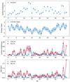 |
Fig. 5. Values of the respective region segments in each map in Fig. 4 are plotted. From top to bottom: surface brightness of the 4−6 keV continuum in units of 10−15 erg s−1 cm−2 arcsec−2; the 4−6 keV energy index, α; surface brightness of cold Fe (6.4 keV, in blue) and hot Fe (Fe XXV at 6.67 keV, in red) in units of 10−9 ph s−1 cm−2 arcsec−2; and EW of cold Fe (6.4 keV) and hot Fe (6.67 keV) in units of keV. |
The Fe XXV EW map in Fig. 4 shows an excess morphology similar to that of the surface brightness but extends further to larger radii in both northern and southern directions. Curiously, these extensions appear to originate from a particular region in the disc. These excesses show EW ranging from 0.2 keV to 0.6 keV and includes dX37 which shows an exceptionally large EW of ∼1.9 keV. More interesting, however, are the small EWs observed in a number of segments. Some of them even have no Fe XXV detection with the EW upper limits of 0.1 keV, despite of having source counts comparable to the other segments. If the diffuse emission is homogeneous gas, then individual segments are expected to have a constant Fe XXV EW of 0.38 keV as measured in the whole diffuse emission spectrum (Table 2). Assuming that the line counts follow a Poisson distribution, the observed EWs would be found in the 0.2−0.6 keV range at a probability of 90%, given the observed counts (eight counts in the line, on average, was assumed). The fact that 17 segments have Fe XXV EW < 0.2 keV, as opposed to an expected 2 (equivalent to ∼5% of the total 38 segments), indicates that the observed EW variations are statistically significant. This spatially biased distribution of Fe XXV means that a significant portion of the diffuse emission areas are void of Fe XXV or have much weaker Fe XXV emission than that seen in the average spectrum. This suggests a presence of a featureless continuum component of non-thermal emission.
As for cold Fe line at 6.4 keV, its brightness CDFs are, in contrast, similar between north and south (Fig. 6). We note that there are two brightest segments, one each in the northern and southern segments, and the shape of the CDFs suggests that the total cold Fe flux is dominated by a small number of bright segments: the brightest five segments compose ≈40% of the total 6.4 keV line flux. The EW of the cold Fe line is similarly balanced between the north and south. There are 12 segments of > 90% detection of cold Fe line. Their EWs are clustered in the 0.16−0.3 keV range with an exception of 0.56 keV from dX28. If their distribution follows a normal distribution (the mean of 0.27 keV and standard deviation of 0.1 keV), two more segments with smaller EWs (< 0.16 keV) are expected to join this distribution if the observation sensitivity was not limited. Therefore ∼40% (14/38) of the segments exhibit cold Fe lines with this moderately large EW of 0.1−0.5 keV. These segments spread over the whole ellipse region, suggesting a diffuse nature of the cold Fe line. We discuss its origin later. Because of the large difference in ionisation stage (and line excitation mechanisms) from Fe XXV, it is no surprise to find different spatial distributions between their brightness and EWs.
 |
Fig. 6. Separate CDFs of the surface brightness of the 4−6 keV continuum, Fe XXV and cold Fe (from left to right) in the northern (N, blue circles) and southern (S, red triangles) parts with respect to the starburst disc plane. These plots were made, using 29 segments with the 4−6 keV surface brightness cut (see text). The 4−6 keV continuum surface brightness is in units of 10−15 erg s−1 cm−2 arcsec−2 while the Fe line surface brightness is in units of 10−8 ph s−1 cm−2 arcsec−2. |
3.3.3. Remarkably strong Fe XXV in dX37
The spectrum of dX37 shows an Fe XXV line with an exceptionally large EW of 1.9 keV (Fig. 5). The Fe K band spectrum shows only the Fe XXV line at  keV but no 6.4 keV line (the 90% upper limit of EW 0.35 keV). The 4−7.2 keV spectrum can be described by an apec model with a temperature of kT = 3.3 ± 0.9 keV and metallicity of
  , which is essentially that of Fe. The temperature is relatively low, compared to the other regions, resulting in the steep continuum slope (α ≃ 2.0; Fig. 5). Lowering a temperature leads to a larger Fe line EW at given metallicity (see Appendix A) but this pronounced line EW is well beyond the effect of varying temperature. The line EW is a factor of ∼5 larger than that of the mean spectrum, and is comparable or even larger than those observed in the spectra of X-ray SNRs selected in Iwasawa (2021).
As described in Sect. 3.3.1, this segment contains the transient source Xp11. However, as the image taken from the same time intervals used to construct the spectrum, that is the transient’s quiescence state, shows no point-like source (Appendix C). No other discrete source, for example, a SNR, is present. No radio SNR is found in the segment either. The 4−6 keV continuum surface brightness is comparable to or even slightly lower than the adjacent segments, dX8 and dX9, located at the similar latitude from the disc. The 6.55−6.9 keV narrow-band image shows a flat distribution of counts within dX37, supporting the diffuse nature of the Fe XXV emission.
An unlikely local metallicity enhancement could boost the line EW, but in the absence of any SN generating objects, such as a star cluster, that coincides with the region which lies ∼90 pc above the molecular disc plane, it does not seem to be the case. Incidentally, the Fe metallicity found in this spectrum is close to ZFe ≃ 2 Z⊙ expected for the metal-rich hot gas with the best estimate of mass loading by Strickland & Heckman (2009). This leads to a possibility that we might happen to see nearly pure emission from the hot gas component in this region with a minimal contribution of non-thermal emission which dominates everywhere else. This possibility is further explored below (Sect. 4).
3.3.4. Relation between continuum slope and Fe XXV strength
Among the measured features, we noted a possible correlation between Fe XXV EW and continuum slope (Fig. 7). Although the data are noisy and the correlation cannot be firmly established, six EWs of Fe XXV larger than 0.5 keV, for example, occur only when the 4−6 keV slopes are α ≥ 1.5 while the median slope of all the spectra is  .
.
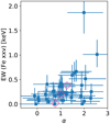 |
Fig. 7. Plot of EW (Fe XXV) against continuum slope α of the 38 region segments (in blue filled-squares). The three magenta diamonds indicate the points for the EW-binned spectra (Table 3), where EW value of each point is the median of EWs measured in the spectra that went into each bin. |
Given the Fe XXV EW variation (from < 0.1 keV to 1.9 keV) examined above, an inclusion of non-thermal emission in addition to the thermal emission characterised by Fe XXV can provide an explanation. In this hypothesis, varying composition of the two components across the diffuse emission region leads to the Fe XXV EW variations. If the non-thermal emission has a harder spectrum than the thermal emission, a spectral slope of a composite spectrum varies as a function of Fe XXV EW, as hinted above. We tested this by inspecting spectra binned into three Fe XXV EW intervals, excluding dX37 with the exceptionally strong Fe XXV. The three EW intervals were set as follows: ‘low’, EWs ≤ 0.15 keV; ‘medium’, 0.15 keV < EWs ≤ 0.3 keV; and ‘high’, 0.3 < EWs ≤ 1 keV (Table 3) and averaged spectra from the three EW bins were obtained. Their spectra, together with the dX37 spectrum as a comparison, are shown in Fig. 8. The spectra from the three bins have background-corrected counts of 0.9−7.5 keV: 59 645 (4−7.5 keV: 2972), 56 247 (3730) and 61 650 (3113) for the low, medium and high EW bins. Their mean fluxes are comparable to one another as well as the quality of their spectra. The 5.4−7.4 keV band centred on the Fe K line complex of the spectra is also shown.
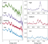 |
Fig. 8. Spectral variations as a function of Fe XXV EW. Left: The broad band spectrum of dX37, integrated spectra of Fe XXV EW of EW ≥ 0.3 keV, 0.15–0.3 keV, and < 0.15 keV (‘high’, ‘medium’, and ‘low’ from top to bottom). Each spectra has been multiplied arbitrarily for displaying purpose. Right: The Fe K band data of the high, medium, and low spectra in the left panel. The flux density is in units of 10−14 erg s−1 cm−2 keV−1. |
Fe XXV EW sliced spectra.
The three spectra are nearly identical in the soft X-ray band up to the Ca K line complex at ∼4 keV, except for small variations at the lowest energies due to varying absorption across the region which correlates with the dust lanes visible in the optical image. This confirms homogeneous emission of the soft X-ray wind covers the entire hard-band diffuse emission region in foreground.
In contrast, the Fe K band spectra are dramatically different between them. The continuum slopes of the three spectra measured in the 4−6 keV band are given in Table 3. The continuum steepens as increasing EW bins (overplotted also in Fig. 8). This trend continues with the even steeper slope found in the dX37 spectrum (Table 3). This agrees with the idea that Fe XXV EW is observed to be small when a contribution of non-thermal emission increases and vice versa.
3.4. Light distribution in 4–8 keV
To measure the approximate shape of the 4−8 keV diffuse light, we took projected light profiles along both the major and minor axes of the galactic disc as shown in Fig. 9. Along the major axis (PA = 70°), one strip labelled as ‘major-Disc’ goes through the molecular disc while the other strip, ‘major-N’, lies ∼70 pc above the disc plane in the middle. The strips are inevitably disrupted by the discrete sources which were masked out. Two strips along the minor axis, ‘minor-E’ and ‘minor-Centre’, are also placed. The reference (zero) point of all the strips is the position of SN2008iz (RA = 09h55m51 55, Dec =
  ; Brunthaler et al. 2009), which is roughly coincides with the FIR emission peak (see Sect. 3.6). Background-corrected 4−8 keV counts were collected from each rectangular region and the surface brightness profiles along each strip was constructed.
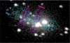 |
Fig. 9. Image of the 4−8 keV emission overlaid by the two strips along the major axis: ‘Disc’ and ‘N’, and the two strips along the minor axis: ‘Centre’ and ‘E’. |
On inspecting those projected profiles, the brightness peak can be located at around the reference point. The light distribution along the major axis is relatively flat and skewed towards the east (Fig. 10a). Along the minor axis, the light distribution is nearly symmetric at the brighter inner part, as already seen in the 4−6 keV map (Fig. 4), but shows an enhanced extension towards north at the fainter brightness level (Fig. 10b). Along each axis, the profile shapes of the two strips are found to be similar, as shown in the standardised brightness plots (Fig. 10c), while their absolute fluxes differ.
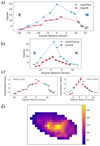 |
Fig. 10. Light distribution in the 4−8 keV band. (a) The 4−8 keV projected light profiles along the major axis taken from the strips shown in Fig. 9. (b) The profiles along the minor axis. (c) These two panels show the same profiles but standardised for a comparison of their shapes. (d) The 4−8 keV diffuse emission image, constructed by two-dimensional interpolation from the point source masked image. Each pixel has an ≈2 × 2 arcsec2 size and the colour bar indicates the brightness scale in units of counts per pixel. |
Another purpose of creating these projected light profiles is to estimate a flux of the diffuse emission in the masked area of the clustered ULXs and other sources, Xp12 though Xp17. By interpolating the four profiles, the 4−8 keV flux in the area was estimated to be ≈3.3 × 10⁻¹³ erg s−1 cm−2, by assuming the same counts-to-flux conversion factor obtained for the diffuse emission spectrum in Sect. 3.2. A two-dimensional interpolation can also be applied directly to the 4−8 keV image with the point source mask used for the 4−6 keV image in Fig. 1. For estimating a missing light profile of the relatively large masked area, we adapted a wide grid-interval and thus the image was re-binned by four pixels before applying the interpolation (interpolation.griddata from Scipy) with the ‘cubic’ method. The resulted interpolated image is shown in Fig. 10d. The missing flux of the masked area, computed from this map, agrees with the above estimate.
3.5. Diffuse emission luminosity
In addition to the ULX area, the expected diffuse flux from the other masked areas of discrete sources was computed by applying the same conversion factor and it is found to be 0.9 × 10⁻¹³ erg s−1 cm−2. Adding these estimated fluxes from the masked areas to the 7.2 × 10⁻¹³ erg s−1 cm−2 of the diffuse emission spectrum (Sect. 3.2), the total 4−8 keV flux of diffuse emission in the ellipse in Fig. 1 is thus 1.1 × 10⁻¹² erg s−1 cm−2, which corresponds to the 4−8 keV luminosity of 1.7 × 1039 erg s−1.
This luminosity, however, contains some contribution of unresolved discrete sources, that is, X-ray binaries and SNRs. We estimated their contributions using the cumulative luminosity distribution, N(> L), which can be approximated by a power-law form (∝L−γ). For X-ray binaries in star-forming galaxies, γ ≃ 0.6 has been found (Colbert et al. 2004; Grimm et al. 2003; Mineo et al. 2012). As γ < 1 implies that brighter sources dominate, fainter, unresolved X-ray binaries have a minor contribution to the observed diffuse emission luminosity anyway. The N(< L) of the X-ray binaries detected by Iwasawa (2021) down to 1 × 10⁻¹⁴ erg s−1 cm−2 in the 4−8 keV band, below which the detection completeness declines rapidly, within the diffuse emission region (excluding the far more luminous ULXs) also show γ ∼ 0.6. Using this slope, we estimated the 4−8 keV luminosity of unresolved X-ray binaries to be 2.0 × 1038 erg s−1. The N(< L) slope for X-ray SNRs appears to have a similar value γ = 0.6 − 0.7, based on the seven X-ray SNRs (Iwasawa 2021). The 4−8 keV luminosity from unresolved X-ray SNRs was then found to be 0.4 × 1038 erg s−1.
A further correction needed is for photons spilled over from the masked discrete sources. About 10% of each discrete source counts in the PSF wing fall outside the masked aperture, on average. This is estimated to be ∼0.6 × 1038 erg s−1. Taking all these into account, the net diffuse emission luminosity in the 4−8 keV band is found to be 1.4 × 1039 erg s−1, in which 1.3 × 1039 erg s−1 comes from the continuum (approximately 9% of the 4−8 keV luminosity originates in Fe XXV). Unless this luminosity solely originates in thermal emission described by the apec fit and in a spheroid as marked by the ellipse in Fig. 1, the mean electron density would be ne ∼ 0.6 cm−3, as the volume of the spheroid is ∼7.9 × 10⁷ pc3.
Strickland & Heckman (2007) estimated the 2−10 keV continuum luminosity of 4.4 × 1039 erg s−1, which corresponds to 2.0 × 1039 erg s−1 in the 4−8 keV band. Our estimate is lower than theirs by about one third. The difference might be attributed to more rigorous removal of discrete sources, including the X-ray SNRs, with the much deeper imaging.
3.6. X-ray, FIR, and radio images
The spatial variation of Fe XXV investigated in Sect. 3.3 led us to consider the hypothesis that the 4−8 keV diffuse emission might be a composite of thermal and non-thermal emission. The non-thermal emission, in this case, arises from inverse Compton scattering of FIR photons by (sub-GeV) cosmic ray electrons (Hargrave 1974). Ample FIR emission is radiated from the dusty starburst region while the cosmic rays are accelerated by SNRs that are abundant in the same region. The electron population of the latter is represented by the synchrotron radio emission. Therefore if this inverse Compton emission is responsible for the diffuse X-ray emission, its morphology is expected to match that at the FIR and radio wavelengths.
We used the FIR image (Fig. 11) taken by the Herschel PACS (Bendo et al. 2012, data were obtained through NED) for a comparison. It provides a 70 μm image at the angular resolution of  (PACS Handbook 2019, version 4.01 ESA). A similar image at 59 μm (the beam FWHM of
  ) has been also taken by SOFIA (Jones et al. 2019). We used a radio continuum image (Fig. 11) taken by the VLA at 3 cm (Adebahr et al. 2013) with D-configuration with a matching beam size (
 ) to the FIR image. The radio continuum at 3-cm represents the high-frequency part of the synchrotron emission with a power-law spectrum ν−0.7 in the starburst region while the electron population responsible for the Compton scattering are attributed to those at lower frequencies (e.g. Strickland & Heckman 2007). The power-law spectrum shows a turnover below 1 GHz due to free-free absorption (Adebahr et al. 2013), meaning that any image taken at frequencies lower than 1 GHz is affected by the absorption which suppresses the brightness in the high obscuration region. For this reason, the high-frequency image is expected to represent the intrinsic distribution of the cosmic ray electron energy density.
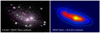 |
Fig. 11. Diffuse X-ray, FIR, and radio image comparison. Left: The 4−8 keV Chandra image in grey-scale overlaid by the Herschel-PACS 70 μm FIR contours in magenta. Right: The PACS 70 μm image overlaid by VLA 3-cm continuum (Adebahr et al. 2013) contours in green. The beam sizes of the PACS and the VLA images are ∼5.5 arcsec and 7.6 × 7.3 arcsec, respectively. Both contours are drawn in seven levels divided in linear scale with the lowest contour corresponding to 10% of the peak brightness in the respective images. |
The FIR and radio images are, unsurprisingly, very similar (Fig. 11 right). Their image morphology agrees well with that of the 4−8 keV diffuse emission (Fig. 11 left; see also Fig. 10d). The matching morphology between the three band images is encouraging for the inverse Compton scattering origin for non-thermal emission. A likely contribution of this non-thermal component to the 4−8 keV continuum luminosity is further discussed in Sect. 4.
3.7. Galactic centre source
The 2.2 μm peak (Lester et al. 1990) has often been assumed to be the galactic centre position of M 82, as the near-IR emission is a good tracer of stellar population and relatively robust against obscuration. However, the K-band emission has a complex structure (see e.g. Alonso-Herrero et al. 2003) and the large X-ray absorbing column of NH ∼ 1023 cm−2 suggests that obscuration could affect the K-band peak position. Instead, there are a few measurements of a kinematic centre determined by H I (Weliachew et al. 1984), [Ne II] (Achtermann & Lacy 1995), and radio H92α line (Rodriguez-Rico et al. 2004) observations. We noted that the X-ray source, Xp9, detected in Iwasawa (2021)3 is located at the radio kinematic centre, and has a relatively faint radio counterpart. The radio source is catalogued as ‘43.21+61.3’ in Rodriguez-Rico et al. (2004) who observed with VLA at 8.3 GHz and 43 GHz and detected with 4 mJy in both frequencies. It is tentatively classified as a H II region because of the flat spectrum. These positions, including the previously measured 2.2 μm peak positions (Rieke et al. 1980; Lester et al. 1990) and the WISE position (Jarrett et al. 2019; WXSC) are plotted over the 2MASS Ks band image (Fig. 12, retrieved from the 2MASS Image Service of IRSA). The positions of Xp9 and the radio source agree with the kinematic centre measurements and the WISE position, and is ≲1″ off to the west from the 2MASS peak. This positional coincidence with the kinematic centre, albeit being tentative, offers a possibility that Xp9 might be a low-luminosity AGN sitting at the galactic centre of M 82. This possibility is examined in Sect. 4.7.
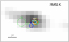 |
Fig. 12. Ks band image of the M 82 nuclear peak emission obtained from 2MASS in grey scale (fainter emission is cut out), overplotted by positions of the X-ray source, Xp9 (white), radio source 43.21+61.3 (red; Rodriguez-Rico et al. 2004), H I kinematic centre (green; Weliachew et al. 1984), Ne II kinematic centre (blue; Achtermann & Lacy 1995), H92α ring centre (cyan; Rodriguez-Rico et al. 2004), WISE peak (yellow; Jarrett et al. 2019), and two previous 2.2 μm peak measurements (R80: Rieke et al. 1980; L90: Lester et al. 1990). The positional error is ∼0.5″ for each measurement, which is represented by the circle, apart from the 2.2 μm position of Rieke et al. (1980). The image orientation is north up, east to the left. |
4. Discussion
We discuss the origin of the diffuse 4−8 keV emission which appears to be composed of multiple components of distinct origins. Three lines of evidence below suggest the presence of significant non-thermal emission in the 4−8 keV diffuse emission: (1) substantial portions of the diffuse emission region exhibit weak or no Fe XXV in the spectrum (Sect. 3.3.2); (2) the continuum hardening with decreasing Fe XXV EW (Sect. 3.3.4); and (3) the morphological resemblance between the X-ray, FIR and radio images (Sect. 3.6). Based on this argument, we present a spectral decomposition of the diffuse X-ray emission that includes inverse Compton emission, followed by a discussion of the inverse Compton emission, metal-rich hot gas, its feedback on ISM and relation to the X-ray SNRs, the 6.4 keV Fe line, and the galactic centre source.
4.1. Composition of the 4–8 keV diffuse emission
Our hypothesis is that the diffuse emission is inverse Compton emission and soft X-ray wind emission, added to the hot gas of kT ∼ 5 keV which occupies specific regions where the Fe XXV line is detected. Based on this picture, we tried to assess the components of the 4−8 keV diffuse emission. We have to consider at least three continuum components: (1) IC: the inverse Compton emission; (2) Th1: the high-energy tail of the soft X-ray wind emission; and (3) Th2: the thermal emission giving rise to the Fe XXV line. As it is not practical to fit all the parameters of such a complex model, we assumed reasonable spectral parameters for each component as described below.
The inverse Compton emission component (IC) is modelled by a power-law. As the spectral slope is expected to be approximately the same as the radio synchrotron spectrum, we assumed the energy index of α = 0.7. This component has the hardest spectrum among the three components.
The soft X-ray wind emission (Th1) is modelled by apec with kT = 1.2 keV. This component, which dominates in the soft X-ray band, should still have a significant contribution in continuum emission at energies around 4−5 keV. The assumed temperature (and also the adopted NH value) was that obtained for the S K band (Fig. 3). We believe this choice is adequate for the soft X-ray wind emission spectrum at energies of Ar K and Ca K emission and above 4 keV for the reason described in Sect. 3.2.1. The metallicity is assumed to be 1 Z⊙ for the following reasons. It has to be larger than 0.6 Z⊙ inferred from the soft X-ray lines (Fig. 3) to compensate the extra continuum contribution of the IC component. With this temperature, the spectrum has high-ionisation Fe K emission including Fe XXV, centred at 6.63 keV (see Appendix A) and it should not overproduce the Fe XXV feature of the ‘low’ spectrum, in which the hot thermal emission (as described below) contribution is supposed to be negligible.
The hot thermal emission (Th2) is modelled by apec with a variable temperature around kT = 5 keV. The Fe metallicity is a key quantity: since this component is the primary source of the observed Fe XXV line (and also Fe XXVI). If the Fe metallicity were known, the continuum strength would automatically be determined. However, we do not know it a priori. Since the reverse is also true and the continuum level, which is driven by the IC component strength, mediates the Fe metallicity, we exploited this route to constrain the Fe metallicity, as below. Strickland & Heckman (2007) derived the original SN ejecta to have Fe metallicity of 5 Z⊙ through a Starburst99 (Leitherer et al. 1999) simulation. This value can be considered as the upper bound and coincides also with the upper bound of the apec model parameter. The lower bound is 1 Z⊙, since the Th1 component is mass-loaded further to the hot fluid by entraining ISM and therefore has lower metallicity than that of Th2.
All these components are assumed to be modified by cold absorption of NH = 2 × 1022 cm−2. The two additional lines at 4.5 keV and 6.4 keV, which are required to describe the data (Sect. 3.2) but not of our interest here, were added as narrow Gaussians.
The three Fe XXV EW sliced spectra in Sect. 3.3.4 (Fig. 7 and Table 3) have continuum slopes that depends on their line EWs. The dX37 spectrum with the exceptionally large Fe XXV EW follows the same trend. We assessed the composition of the three continuum components that can reproduce their varying spectral slopes, which, in turn, constrains the Fe metallicity of Th2. The ‘low’ Fe XXV EW spectrum can be considered to have a negligible contribution of Th2, as its weak Fe XXV line can be accounted for solely by Th1. On the contrary, the dX37 spectrum should be dominated by Th2. We fitted the three EW-sliced spectra and dX37 spectrum in the 4−7.2 keV band jointly, leaving the normalisation of each component and the temperature and (Fe) metallicity of Th2 as free parameters.
This fit gives a good description of the data with C-stat. = 785.3 with 774 bins (754 d.o.f.). The temperature was found to be kT = 5.0 ± 0.8 keV. The best-fit Fe metallicity was driven to the highest bound of 5 Z⊙ but the likelihood remains similar above 2.5 Z⊙ (Fig. 13). This can be compared with the Fe metallicity of ∼2 Z⊙, which would be expected from the best-estimate of the mass-loading factor of 2.7 by Strickland & Heckman (2009).
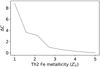 |
Fig. 13. C-statistic curve for the Fe metallicity of Th2 in the joint fit of the three EW-sliced spectra and dX37 spectrum with the three continuum component model. |
We computed 4−8 keV fluxes of the IC, Th1 and Th2 components in the four EW-sliced spectra, adopting the Th2 Fe metallicity of 3.8 Z⊙, which is the probability-weighted mean over the expected metallicity range of 1−5 Z⊙. Their proportions of the total 4−8 keV flux in each spectrum are given in Table 4 (where the contribution of the 4.5 keV and 6.4 keV lines are left out). With the same set of spectral components, a spectral decomposition for the total diffuse emission spectrum (Fig. 2) is illustrated in Fig. 14. The relative contributions of the respective components are also given in Table 4.
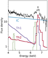 |
Fig. 14. Same spectrum shown in Fig. 2 with the best estimate of the three continuum components, IC (blue), Th1 (purple) and Th2 (red) assuming the Fe metallicity of Th2 to be 3.8 Z⊙. Two additional lines at 4.5 keV and 6.4 keV are also plotted in dotted lines. The flux density is in units of 10−14 erg s−1 cm−2 keV−1. |
4−8 keV flux compositions.
We note that the Fe K line at 6.67 keV is actually a sum of the lines from Th1 and Th2. The Fe K feature of Th1 is centred at 6.63 keV, consisting of Fe XXV and weaker lines originating in lower ionisation stages, given the temperature of kT = 1.2 keV. This Th1 contribution probably shifts the line centroid and broadens the width to the observed 6.67 keV and σ = 0.05 keV (Table 2) from 6.68 keV and σ = 0.03 keV, expected from a kT = 5 keV plasma.
The IC flux correlates weakly with the Fe metallicity via the Th2 continuum flux. In the probable 2.5−5 Z⊙ range, the IC component carries 66−70% (±3%) of the 4−8 keV diffuse emission luminosity, which corresponds to (0.9−1) × 1039 erg s−1. This, however, contains the contribution of unresolved X-ray binaries with a similar spectral shape, which was estimated to be 0.2 × 1039 erg s−1 (Sect. 3.5). Correcting for this, the net 4−8 keV luminosity of inverse Compton emission is (0.7−0.8) × 1039 erg s−1.
4.2. Inverse Compton emission
The parameters for estimating the energy loss of cosmic ray electrons due to inverse Compton scattering were obtained by Adebahr et al. (2013), using their radio data, combined with the FIR data from AKARI. They agree with those used by Persic et al. (2008) who predicted a 2−10 keV flux of IC X-ray emission, which assumed that the entire FIR emission (measured with IRAS) comes from radii ≤300 pc. However, since some fraction extends out, as shown in the AKARI (Kaneda et al. 2010) and Herschel (Contursi et al. 2013) images, a correction is needed to obtain the FIR energy density for the X-ray diffuse emission region. The LFIR of the central < 1′ in radius is 2.4 × 1043 erg s−1, estimated using the Helou et al. (1988) formula with S60 = 630 Jy and S100 = 529 Jy, measured with AKARI-FIS (Kaneda et al. 2010). We found, from the PACS 70 μm image, that ≈60% of this luminosity comes from the ellipse of the X-ray diffuse emission. Weighting with the FIR emission distribution, the mean FIR energy density within the ellipse was estimated to be UFIR ∼ 0.82 × 10⁻⁹ erg cm−3. Adebahr et al. (2013) derived the magnetic field strength of B = 98 μG of the M 82 central region, using the revised equipartition formula of Beck & Krause (2005). It is slightly smaller than 106 μG of Persic et al. (2008) but has an uncertainty of ±30% due to the assumed proton to electron number density ratio. The slope of the radio spectrum is assumed to be α = −0.7, as in Sect. 3.6. This corresponds to the cosmic ray electron spectrum in terms of Lorentz factor γ: Ne(γ)∝γ−2.4. FIR photons at 70 μm, for example, are up-scattered to the 4−8 keV range by γ ∼ 500 − 700. Following Persic et al. (2008) with these conditions, the expected 4−8 keV IC luminosity is found to be 0.6 × 1039 erg s−1. This agrees with the decomposed IC emission luminosity found above.
4.3. Metal-rich hot gas
Even given its small contribution to the continuum emission, the thermal emission from the hot gas of kT ≃ 5 keV is the source of the majority of Fe XXV line, as shown above, and can be traced by the enhanced Fe XXV EW (Fig. 4). The map shows that the presence of the hot gas component is limited within a small distance from the starburst disc and seen to be much stronger on the northern side, suggesting an asymmetric ejection of hot gas.
A northern asymmetry in outflow structures have also been observed in other wavelengths. In the mid-infrared (mid-IR) image taken by the Subaru-COMICS with the [Ne II] filter at 12.8 μm, a few wisps are seen only on the northern side, extending from the starburst disc (Gandhi et al. 2011). The same features are noted also in radio. Figure 16 shows the deep JVLA image of the central part of M 82 at 3-GHz, taken on 2015 August 16. The overlaid COMICS contours shows the coincidence of the northern wisps between mid-IR and radio. Wills et al. (1999) noted these radio counterparts in the earlier VLA images and identified four galactic chimneys, based on the emission void to the south of the radio SNR 41.95+57.5. Here, we refer to a chimney as a collimated structure of a super bubble breaking out of the galactic disc. The primary energy source here is a sequence of SNe produced by a starburst and its formation has been formulated by earlier study (Tomisaka & Ikeuchi 1986; Mac Low & McCray 1988; Norman & Ikeuchi 1989). The mid-IR and radio emission voids, embraced by the wisps, correspond to chimneys that are expected to be filled by hot gas (Tomisaka & Ikeuchi 1988).
Figure 15 shows that the Fe XXV EW enhancement regions, as indicated by arrows I, II, and III. They appear to fill the mid-IR voids and to be traced back to the mid-IR knot ‘E1’ of Achtermann & Lacy (1995). This can be understood that the metal-rich hot gas produced in the E1 knot was channelled into the chimneys and fills their interior.
 |
Fig. 15. Fe XXV EW map overlaid by the Subaru-COMICS mid-IR [Ne II] contours. The colour bar shows the Fe XXV EW in keV. The white arrows indicates the three Fe XXV-enhanced regions I, II, and III, which appear to fill the chimneys and to be connected to the mid-IR knot ‘E1’ (Achtermann & Lacy 1995). The orange arrow indicates the chimney with an expanding bubble identified around the SNR 41.95+57.5 by Wills et al. (1999). The two region-segments dX34 and dX35, discussed in the text, are also indicated. |
The mean density of the hot gas is found to be n = 0.09 cm−3. We note that if the hot gas does not fill the full diffuse emission volume, the density increases by f−1/2, where f is the filling factor. The pressure of hot gas with kT = 5 keV is then log P ≈ 6.7 [K cm−3]. The hot gas of this temperature has a thermal velocity (∼3000 km s−1) much larger than the galaxy’s escape velocity (∼460 km s−1; Strickland & Heckman 2009) and, consequently, flows out. However, as the dense molecular gas in the starburst disc has a comparable pressure, log P ∼ 6.5 [K cm−3], measured by Naylor et al. (2010), the gas would flow out only in a favourable direction set out by the chimneys.
4.4. Effects of supernova feedback
The recent star formation in M 82 is believed to be triggered by a tidal interaction with M 81 (e.g. Yun et al. 1993), resulting in two short (∼1 Myr) bursts of star formation 5 Myr and 10 Myr ago (Rieke et al. 1993; Förster Schreiber et al. 2003). The first intense burst peaking at the nuclear region was followed by the second burst in a circumnuclear ring. The mid-IR E1 knot is likely clustered H II regions and is associated with the eastern part of the starburst ring, just inside the molecular concentration (Achtermann & Lacy 1995). After the second burst, which had an initial star formation rate (SFR) of ∼43 M⊙ yr−1, the SFR declined rapidly (Förster Schreiber et al. 2003). The present SFR, based on the FIR luminosity (Kennicutt 1998), corrected for the flattened IMF at lower masses (Rieke et al. 2009), is 4.3 M⊙ yr−1 over the mass range of 0.1−100 M⊙.
According to the two-burst model, the starburst ring should have accumulated numerous SNRs but also still keeps producing new SNe. However, some 40 radio SNRs in M 82 all avoid the enhanced star-forming knots. While this has been a subject of discussion in various articles (e.g. Golla et al. 1996; de Grijs 2001; Alonso-Herrero et al. 2003), it could be understood when taking the starburst age and local SN feedback into account. We illustrate it using E1 as an example, since it is part of the starburst ring where the second burst took place 5 Myr ago for a duration of 1 Myr.
In the simplified starburst episode assumed above, as a massive star with a mass of M lives for ∼30(M/8 M⊙)−2.5 Myr, stars with masses of ≳17 M⊙ already died, leaving both SNe and SNRs. Taking the typical SFR surface density 5 × 10⁻⁴ M⊙ yr−1 pc−2 for the second burst (Förster Schreiber et al. 2003), a circular region with a diameter of 3″ gives a SFR of ∼1 M⊙ yr−1 for E1. Then E1 has accumulated some 2000 SNRs at present time. Here we used the SFR to SN rate conversion factor of 0.0088 of Horiuchi et al. (2011). The series of SN explosions produce a hot cavity and its filling factor within the star-forming knot grows as the number of SNe increases (McKee & Ostriker 1977). In this rarefied environment, SNe and SNRs do not cool. This means they directly heat the ambient medium by providing much of the energy in mechanical form and thus could be difficult to detect due to low brightness.
The above process produces metal-rich hot fluid of a temperature of 108 K (Chevalier & Clegg 1985). In our Chandra observations, the region-segment dX34 coincides with the central part of E1 (Fig. 15). The X-ray spectrum of dX34 shows no Fe XXV line (Fig. 5), suggesting that the putative hot fluid, too, radiates little with its low emission measure. On the other hand, abundant amounts of dust are produced by SNe (Gall & Hjorth 2018), providing a source of strong FIR emission. The region also acts as a cosmic ray reservoir, since a significant fraction (∼10%) of SN explosion energy may go efficiently into cosmic ray acceleration (Pais et al. 2018; Grenier et al. 2015; Caprioli & Spitkovsky 2014; Bell et al. 2004). Thus the local SN feedback and dust production together produce IC X-ray emission, which dominates the dX34 spectrum. However, once the metal-enriched hot fluid flows out of E1, it entrains the surrounding cool ISM. This leads to a drop in temperature, as demostrated by simulations (e.g. Tomisaka & Ikeuchi 1988), and an increased density makes the fluid sufficiently radiative, resulting in sub-108 K gas with strong Fe XXV. This transition can be illustrated by the spectrum of dX35, which lies immediately outside E1 and at the base of the south-bound Fe XXV extension III (Fig. 15). The segments dX34 and dX35 are both located in the disc plane and separated by only ∼20 pc, yet the strong Fe XXV line in the dX35 spectrum contrasts sharply with that of dX34 with no Fe XXV.
The above hypothesis explains how, despite lacking detectable SNRs, E1 exhibits the X-ray spectrum dominated by IC emission, yet it acts as a hub of the Fe XXV-enhanced emission. The total energy deposited by 2000 SNe in E1 over the last 5 Myr amounts to ∼2 × 1054 erg. About 10% of this energy would go to cosmic rays, and ∼5% is radiated away via the Fe XXV-emitting hot gas, as observed. Therefore the majority of the SN energy should have gone to the chimney in kinetic form and was transported to the halo.
4.5. Detectability of radio and X-ray SNRs
The brightest five radio SNRs have X-ray counterparts (Iwasawa 2021; see Fig. 16). An inspection of the deep JVLA image found a faint radio source which appears to coincide with another X-ray SNR, Xp17. This makes six X-ray–radio correspondences out of the seven X-ray SNRs detected in Iwasawa (2021), which is remarkably high, compared to those in other nearby galaxies (Leonidaki et al. 2010; Long et al. 2010; Pannuti et al. 2007), suggesting that they share a favourable condition, for example, dense environment, to be highly radiative in both wavelengths. Such a dense environment no longer exists in the interior of the past burst sites, as described above. Instead, freshly formed giant molecular clouds (GMC), whose lifetime could be a few Myr (Dobbs & Pringle 2013), may sustain the present star-forming activity which dispenses young SNRs. In fact, all the seven X-ray SNRs are found to reside within GMCs with masses of 4 × 10³ M⊙ − 1.7 × 10⁷ M⊙, catalogued by Krieger et al. (2021) who mapped them in CO(1−0) with IRAM NOEMA (the median projected distance of those X-ray SNRs from the respective cloud centres is 34 pc while the median cloud radius 54 pc), supporting the above idea. They provide an ideal environment for those young radio and X-ray SNRs which are less than a few hundreds yr old (e.g. Fenech et al. 2010; Iwasawa 2021), since there have been little pre-existing SN feedback. The estimated radio SN rates are in the range of 0.03−0.1 yr−1 (Unger et al. 1984; Kronberg et al. 1985; Muxlow et al. 1994; Huang et al. 1994; Fenech et al. 2008, 2010), corresponding to SFR of 3.4−11 M⊙ yr−1, in agreement with the current SFR. Different manifestations of SN feedback depending on their molecular gas environment, as discussed for nearby star-forming galaxies in the PHANGS survey (Mayker Chen et al. 2023), is also in support of our argument.
 |
Fig. 16. JVLA map at 3 GHz overlaid by the Subaru-COMICS [NII] contours. Three (or four) ‘wisps’ are seen both in mid-IR and radio on the northern side. The green diamond indicates the radio source, 43.21+61.3 of Rodriguez-Rico et al. (2004), which coincides with the X-ray source, Xp9, at the position of the radio kinematic centre. The five brightest radio SNRs, all of which have X-ray counterparts, are encircled in white. The radio SNR 41.95+57.5 (=X-ray SNR, Xp15) and presently the brightest radio SNR of SN2008iz (Brunthaler et al. 2009) are indicated. |
4.6. 6.4 keV cold Fe K line
The origin of the 6.4 keV cold Fe K line is unclear. Liu et al. (2014) argued irradiation of optically thin NH ∼ 1022 cm−2 cold ISM by the luminous X-ray binaries can account for the total line luminosity. The two segments of high surface brightness in 6.4 keV emission (dX14 and 28) near the bright X-ray binary concentration in the western part may fit this scenario. However, the mapped distribution of the line emission suggests its diffuse nature and the extended emission towards the eastern part is difficult to account for by photoionisation of bright X-ray binaries alone.
Here, we examine an alternative line production mechanism by cosmic ray bombardment, which has been proposed for explaining 6.4 keV Fe lines seen in the Galactic centre (Valinia et al. 2000; Dogiel et al. 2009) and the surroundings of some of the Galactic SNRs (Tatischeff et al. 2012). This process is compatible with the diffuse nature of the emission across the starburst region. While the energy density of cosmic ray in M 82 is expected to be high, the line production is inefficient: η = L6.4/LCR ∼ 10−6 at most (Tatischeff et al. 2012). With the SFR = 33 M⊙ yr−1 over the past 15 Myr, the SN rate would be νSN ∼ 0.3 yr−1. Assuming ϵ = 10% of the SN energy (1051 erg per SN) goes to cosmic rays, the efficiency of η = 10−6 gives an expected 6.4 keV line luminosity of ∼1 × 1036(ϵ/0.1)(νSN/0.3 yr−1)(η/10−6) erg s−1, if SNe are the sole accelerator of cosmic rays. This estimate is more than one order of magnitude below the total 6.4 keV line luminosity (Table 2) and cannot be a major source of the detected line emission. Similar to the Galactic centre (Sgr B2 clouds, in particular, Zhang et al. 2015; Rogers et al. 2022; Kuznetsova et al. 2022), while the 6.4 keV line emission of the cosmic ray origin accounts for the low-brightness, extended emission in M 82, the brightest spots need to be explained by irradiation of transient flaring sources, whether they are M 82 X-1 or transient X-2, which can reach LX > 1040 erg s−1 (Kaaret et al. 2001; Brightman et al. 2019), or even an active nucleus, as discussed below. A long term monitoring of the brightest regions can test the photoionisation scenario through variability in line flux.
4.7. Possible AGN at the galactic centre
The previous claim of a low-luminosity AGN in M 82 was based on hard X-ray variability observed with ASCA (Ptak & Griffiths 1999; Matsumoto & Tsuru 1999), which, as we know now, is caused by the ULXs. Here, we examine how plausible the faint X-ray source, Xp9, at the galactic centre might be an AGN. Xp9 has been assumed to be an X-ray binary but the presence of the radio counterpart makes it unique among the X-ray binaries detected in the central region. The deep JVLA image verifies the radio counterpart, as marked by a magenta diamond in Fig. 16, whilst none of the other X-ray binaries (including the ULXs) have a point-like radio counterpart in the JVLA image (Xp6 and Xp16 coincide with compact radio sources but they are radio SNRs; Fenech et al. 2010). An X-ray binary could have a radio jet in the hard state. However, as Galactic black hole binaries typically have radio luminosity LR ≤ 1030 erg s−1 (e.g. Gallo et al. 2012, the micro quasar GRS1915+105 occasionally reaches 1 × 1032 erg s−1, as an exception) in the hard state, no radio detection is expected for X-ray binaries in M 82, in agreement with the lack of radio counterpart of the other X-ray binaries. In contrast, assuming a flat spectrum and 4 mJy at 5 GHz, Xp9 has log LR ≃ 32.5 [erg s−1], which is comparable to that of Sgr A⋆. In the context of the black hole fundamental plane (Merloni et al. 2003), radio luminosity, LR, increases with black hole mass, MBH, and thus the radio loudness of Xp9 points to a large MBH.
The X-ray spectrum of Xp9 is very hard with the power-law slope of α ∼ −1 and the source is visible only above 3 keV. The hard spectrum is likely due to strong absorption: if an intrinsic slope of α = 0.7 is assumed, absorbing column density would be NH ∼ 2 × 1023 cm−2. The observed 4−8 keV flux is 3.0 × 10⁻¹⁴ erg s−1 cm−2 and the absorption-corrected 2−10 keV flux would be 1.2 × 10⁻¹³ erg s−1 cm−2. The latter corresponds to log LX ≃ 38.27 [erg s−1]. The 4−7 keV light curve remains stable over 16 yr of the Chandra observations (Iwasawa 2021). The X-ray luminosity is compatible to a bright X-ray binary but could also be of low-luminosity AGN, powered by an intermediate-mass black hole or a supermassive black hole operating at inefficient accretion flow, such as an advection-dominated accretion flow (ADAF; Narayan & Yi 1994).
Gaffney et al. (1993) obtained the nuclear enclosed mass M (r < 8.5 pc) = 3 × 10⁷ M⊙, using the CO absorption bandhead kinematics (see also Greco et al. 2012). It can be considered as an upper limit of the mass of a putative black hole, MBH. However, MBH ∼ 106 M⊙, similar to that of Sgr A⋆, would be possible only if a significant portion of the stellar disc was stripped away on the close encounter with M 81, leaving M 82 as a bulge-dominated galaxy, as proposed by Sofue (1998), otherwise it is deemed to be overmassive for the galaxy with the total mass of 1010 M⊙ (Greco et al. 2012). With the observed radio and X-ray luminosities, the black hole fundamental plane gives MBH of 103 − 104 M⊙ (Merloni et al. 2003; Gültekin et al. 2019). While whether black holes in this mass range exist is presently unclear, it is compatible with the argument of M 82 to be a bulgeless galaxy (Mayya & Carrasco 2009). Some low-luminosity AGNs hosted by small, bulgeless galaxies, such as NGC 4395, have black hole masses of the order of 105 M⊙ (Peterson et al. 2005). When MBH = 105 M⊙ is assumed, the typical bolometric correction of κ ≡ Lbol/LX = 16 for low-luminosity AGN (Ho 2008) gives the bolometric luminosity of Xp9 to be 3 × 1039(κ/16) erg s−1. Then the Eddington ratio would be λ ∼ 2 × 10⁻⁴(κ/16)(MBH/105 M⊙)−1, well within the ADAF range. The flat radio spectrum is similar to Sgr A⋆ and other sources that are suspected to be operating in ADAF, slightly steeper than ∼0.3 predicted for ADAF (Mahadevan 1997). There is no notable evidence for past elevated AGN activity, such as the Fermi bubble in our Galaxy, although the starburst activity might disguise it.
The radio-to-X-ray spectral energy distribution of Xp9 is shown in Fig. 17. The mid-IR points are upper limits from Gandhi et al. (2011). The 12-μm luminosity predicted by the ADAF models (Mahadevan 1997; Kino et al. 2000) and the mid-IR–X-ray relation of Gandhi et al. (2009) is around 1038 − 1039 erg s−1. This is translated to a flux density of 0.7−7 μJy, which may be barely detectable with the upcoming James Webb Space Telescope-MIRI observation (ID: 1701). As the mid-IR luminosity expected from an X-ray binary is a few orders of magnitude farther down, any detection with JWST would point to the low-luminosity AGN hypothesis.
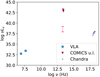 |
Fig. 17. Spectral energy distribution of Xp9. The radio data points are from Rodriguez-Rico et al. (2004). The mid-IR data points are upper limits obtained from the Subaru-COMICS images (Gandhi et al. 2011). The luminosity range at 12 μm, expected from the low-luminosity AGN hypothesis, is indicated by the dotted-line, which could be within the reach of the upcoming JWST observations. |
5. Conclusions
We present the spatially resolved spectral map of the 4−8 keV diffuse emission in M 82 at a few arcsec resolution, after removing point-like sources. Our findings are summarised as follows.
-
The EW of the Fe XXV line from hot gas varies widely across the diffuse emission region, including areas with EW < 0.1 keV, suggesting the presence of non-thermal emission. The morphology of the diffuse X-ray emission resembles those of the FIR and radio emission, in favour of inverse Compton scattering off the FIR photons by cosmic ray electrons as the origin of the non-thermal emission.
-
We found that the 4−8 keV diffuse emission is composed of three spectral components with distinct origins: (1) inverse Compton emission which carries ∼70% of the continuum luminosity in the band; (2) the hard tail of the soft X-ray wind emission of kT ∼ 1 keV; and (3) metal-rich, hot gas emission of kT ∼ 5 keV, which accounts for the majority of the observed Fe XXV line but is a minor component of the continuum.
-
The hot gas, traced by enhanced Fe XXV EW, is found in a limited area near the galactic disc and appears to flow out from the eastern part of the starburst ring and fills the chimneys marked by mid-IR and radio voids. The chimneys dominate in transporting the flow of SN energy from the disc to halo in M 82.
-
The brightest, young X-ray and radio SNRs are found to reside in GMCs that are presumably newly formed and thus free from strong SN feedback. This could explain their positional displacement from the past active star-forming sites where any SN would be little radiative due to the hot, low-density interior.
-
The faint X-ray source, Xp9, located at the galactic centre, is unusual for an X-ray binary to have a luminous radio counterpart with a flat spectrum, offering a possibility to be a low-luminosity AGN with LX ∼ 1038 erg s−1 in an ADAF phase.
A similar technique employed in this work can be applied with advanced future X-ray mission with high angular resolution, such as AXIS or LYNX, to reveal effects of feedback on the ISM in a range of nearby galaxies, including those with central AGN.
apec is the code to calculate a thermal emission spectrum (Foster et al. 2012). Here, gas in a collisional ionisation equilibrium is assumed.
We use energy index, α, for a spectral slope appropriate for a spectrum in flux density unit, as defined as fE ∝ E−α, where fE is flux density and E is energy. The conventional photon index, Γ, is related as Γ = 1 + α.
The source position is 09h55m52.0s, +69d40m47.3s, There was a typo in the Dec in Iwasawa (2021). This is the correct position of Xp9.
Acknowledgments
We thank the referee for helpful comments. This research made use of data obtained from Chandra X-ray Observatory, of which the archive is maintained by Chandra X-ray Center (CXC) and NASA/IPAC Extragalactic Databases (NED) and Infrared Science Archive (IRSA), which are funded by the NASA and operated by the California Institute of Technology. Software packages of CIAO 4.12, HEASoft 6.27.1, Astropy, PyMC, Matplotlib, Numpy, Pandas, Scipy and IPython were used for data analysis. K.I. acknowledges support by grant PID2019-105510GB-C33 funded by MCIN/AEI/10.13039/501100011033 and “Unit of excellence María de Maeztu 2020-2023” awarded to ICCUB (CEX2019-000918-M). M.P.T. acknowledges financial support from the Spanish Ministerio de Ciencia e Innovación (MCIN), the Agencia Estatal de Investigación (AEI) through the “Center of Excellence Severo Ochoa” award to the Instituto de Astrofísica de Andalucía (SEV-2017-0709) and through grant PID2020-117404GB-C21 funded by MCIN/AEI/10.13039/501100011033.
References
- Abdo, A. A., Ackermann, M., Ajello, M., et al. 2010, ApJ, 709, L152 [NASA ADS] [CrossRef] [Google Scholar]
- Achtermann, J. M., & Lacy, J. H. 1995, ApJ, 439, 163 [NASA ADS] [CrossRef] [Google Scholar]
- Adebahr, B., Krause, M., Klein, U., et al. 2013, A&A, 555, A23 [NASA ADS] [CrossRef] [EDP Sciences] [Google Scholar]
- Alonso-Herrero, A., Rieke, G. H., Rieke, M. J., & Kelly, D. M. 2003, AJ, 125, 1210 [CrossRef] [Google Scholar]
- Arnaud, K. A. 1996, ASP Conf. Ser., 101, 17 [Google Scholar]
- Beck, R., & Krause, M. 2005, Astron. Nachr., 326, 414 [Google Scholar]
- Bell, E. F., McIntosh, D. H., Barden, M., et al. 2004, ApJ, 600, L11 [NASA ADS] [CrossRef] [Google Scholar]
- Bendo, G. J., Boselli, A., Dariush, A., et al. 2012, MNRAS, 419, 1833 [NASA ADS] [CrossRef] [Google Scholar]
- Blackburn, J. K., Shaw, R. A., Payne, H. E., et al. 1999, Astrophysics Source Code Library [record ascl:9912.002] [Google Scholar]
- Brightman, M., Harrison, F. A., Bachetti, M., et al. 2019, ApJ, 873, 115 [Google Scholar]
- Brunthaler, A., Menten, K. M., Reid, M. J., et al. 2009, A&A, 499, L17 [NASA ADS] [CrossRef] [EDP Sciences] [Google Scholar]
- Caprioli, D., & Spitkovsky, A. 2014, ApJ, 783, 91 [CrossRef] [Google Scholar]
- Cash, W. 1979, ApJ, 228, 939 [Google Scholar]
- Chevalier, R. A., & Clegg, A. W. 1985, Nature, 317, 44 [Google Scholar]
- Colbert, E. J. M., Heckman, T. M., Ptak, A. F., Strickland, D. K., & Weaver, K. A. 2004, ApJ, 602, 231 [NASA ADS] [CrossRef] [Google Scholar]
- Contursi, A., Poglitsch, A., Graciá Carpio, J., et al. 2013, A&A, 549, A118 [NASA ADS] [CrossRef] [EDP Sciences] [Google Scholar]
- de Grijs, R. 2001, Astron. Geophys., 42, 4.12 [Google Scholar]
- Dobbs, C. L., & Pringle, J. E. 2013, MNRAS, 432, 653 [NASA ADS] [CrossRef] [Google Scholar]
- Dogiel, V., Cheng, K.-S., Chernyshov, D., et al. 2009, PASJ, 61, 901 [NASA ADS] [CrossRef] [Google Scholar]
- Fenech, D. M., Muxlow, T. W. B., Beswick, R. J., Pedlar, A., & Argo, M. K. 2008, MNRAS, 391, 1384 [NASA ADS] [CrossRef] [Google Scholar]
- Fenech, D., Beswick, R., Muxlow, T. W. B., Pedlar, A., & Argo, M. K. 2010, MNRAS, 408, 607 [NASA ADS] [CrossRef] [Google Scholar]
- Förster Schreiber, N. M., Genzel, R., Lutz, D., & Sternberg, A. 2003, ApJ, 599, 193 [CrossRef] [Google Scholar]
- Foster, A. R., Ji, L., Smith, R. K., & Brickhouse, N. S. 2012, ApJ, 756, 128 [Google Scholar]
- Freedman, W. L., Hughes, S. M., Madore, B. F., et al. 1994, ApJ, 427, 628 [NASA ADS] [CrossRef] [Google Scholar]
- Fruscione, A., McDowell, J. C., Allen, G. E., et al. 2006, SPIE Conf. Ser., 6270, 62701V [Google Scholar]
- Gaffney, N. I., Lester, D. F., & Telesco, C. M. 1993, ApJ, 407, L57 [NASA ADS] [CrossRef] [Google Scholar]
- Gall, C., & Hjorth, J. 2018, ApJ, 868, 62 [CrossRef] [Google Scholar]
- Gallo, E., Miller, B. P., & Fender, R. 2012, MNRAS, 423, 590 [Google Scholar]
- Gandhi, P., Horst, H., Smette, A., et al. 2009, A&A, 502, 457 [NASA ADS] [CrossRef] [EDP Sciences] [Google Scholar]
- Gandhi, P., Isobe, N., Birkinshaw, M., et al. 2011, PASJ, 63, 505 [Google Scholar]
- Golla, G., Allen, M. L., & Kronberg, P. P. 1996, ApJ, 473, 244 [NASA ADS] [CrossRef] [Google Scholar]
- Greco, J. P., Martini, P., & Thompson, T. A. 2012, ApJ, 757, 24 [NASA ADS] [CrossRef] [Google Scholar]
- Grenier, I. A., Black, J. H., & Strong, A. W. 2015, ARA&A, 53, 199 [Google Scholar]
- Griffiths, R. E., Ptak, A., Feigelson, E. D., et al. 2000, Science, 290, 1325 [CrossRef] [Google Scholar]
- Grimm, H. J., Gilfanov, M., & Sunyaev, R. 2003, MNRAS, 339, 793 [Google Scholar]
- Gültekin, K., King, A. L., Cackett, E. M., et al. 2019, ApJ, 871, 80 [Google Scholar]
- Hargrave, P. J. 1974, MNRAS, 168, 491 [NASA ADS] [CrossRef] [Google Scholar]
- Helou, G., Khan, I. R., Malek, L., & Boehmer, L. 1988, ApJS, 68, 151 [NASA ADS] [CrossRef] [Google Scholar]
- Ho, L. C. 2008, ARA&A, 46, 475 [Google Scholar]
- Horiuchi, S., Beacom, J. F., Kochanek, C. S., et al. 2011, ApJ, 738, 154 [NASA ADS] [CrossRef] [Google Scholar]
- Huang, Z. P., Thuan, T. X., Chevalier, R. A., Condon, J. J., & Yin, Q. F. 1994, ApJ, 424, 114 [NASA ADS] [CrossRef] [Google Scholar]
- Iwasawa, K. 2021, A&A, 652, A18 [NASA ADS] [CrossRef] [EDP Sciences] [Google Scholar]
- Jarrett, T. H., Cluver, M. E., Brown, M. J. I., et al. 2019, ApJS, 245, 25 [Google Scholar]
- Jones, T. J., Dowell, C. D., Lopez Rodriguez, E., et al. 2019, ApJ, 870, L9 [NASA ADS] [CrossRef] [Google Scholar]
- Kaaret, P., Prestwich, A. H., Zezas, A., et al. 2001, MNRAS, 321, L29 [Google Scholar]
- Kaneda, H., Ishihara, D., Suzuki, T., et al. 2010, A&A, 514, A14 [NASA ADS] [CrossRef] [EDP Sciences] [Google Scholar]
- Kennicutt, R. C., Jr 1998, ARA&A, 36, 189 [NASA ADS] [CrossRef] [Google Scholar]
- Kino, M., Kaburaki, O., & Yamazaki, N. 2000, ApJ, 536, 788 [NASA ADS] [CrossRef] [Google Scholar]
- Krieger, N., Walter, F., Bolatto, A. D., et al. 2021, ApJ, 915, L3 [NASA ADS] [CrossRef] [Google Scholar]
- Kronberg, P. P., Biermann, P., & Schwab, F. R. 1985, ApJ, 291, 693 [CrossRef] [Google Scholar]
- Kuznetsova, E., Krivonos, R., Lutovinov, A., & Clavel, M. 2022, MNRAS, 509, 1605 [Google Scholar]
- Leitherer, C., Schaerer, D., Goldader, J. D., et al. 1999, ApJS, 123, 3 [Google Scholar]
- Leonidaki, I., Zezas, A., & Boumis, P. 2010, ApJ, 725, 842 [NASA ADS] [CrossRef] [Google Scholar]
- Lester, D. F., Carr, J. S., Joy, M., & Gaffney, N. 1990, ApJ, 352, 544 [NASA ADS] [CrossRef] [Google Scholar]
- Liu, J., Gou, L., Yuan, W., & Mao, S. 2014, MNRAS, 437, L76 [NASA ADS] [CrossRef] [Google Scholar]
- Long, K. S., Blair, W. P., Winkler, P. F., et al. 2010, ApJS, 187, 495 [NASA ADS] [CrossRef] [Google Scholar]
- Mac Low, M.-M., & McCray, R. 1988, ApJ, 324, 776 [NASA ADS] [CrossRef] [Google Scholar]
- Mahadevan, R. 1997, ApJ, 477, 585 [NASA ADS] [CrossRef] [Google Scholar]
- Matsumoto, H., & Tsuru, T. G. 1999, PASJ, 51, 321 [NASA ADS] [CrossRef] [Google Scholar]
- Mayker Chen, N., Leroy, A. K., Lopez, L. A., et al. 2023, ApJ, 944, 110 [NASA ADS] [CrossRef] [Google Scholar]
- Mayya, Y. D., & Carrasco, L. 2009, Rev. Mex. Astron. Astrofis. Conf. Ser., 37, 44 [NASA ADS] [Google Scholar]
- McKee, C. F., & Ostriker, J. P. 1977, ApJ, 218, 148 [NASA ADS] [CrossRef] [Google Scholar]
- Merloni, A., Heinz, S., & di Matteo, T. 2003, MNRAS, 345, 1057 [Google Scholar]
- Mineo, S., Gilfanov, M., & Sunyaev, R. 2012, MNRAS, 419, 2095 [Google Scholar]
- Moran, E. C., & Lehnert, M. D. 1997, ApJ, 478, 172 [NASA ADS] [CrossRef] [Google Scholar]
- Muxlow, T. W. B., Pedlar, A., Wilkinson, P. N., et al. 1994, MNRAS, 266, 455 [NASA ADS] [CrossRef] [Google Scholar]
- Narayan, R., & Yi, I. 1994, ApJ, 428, L13 [Google Scholar]
- Naylor, B. J., Bradford, C. M., Aguirre, J. E., et al. 2010, ApJ, 722, 668 [NASA ADS] [CrossRef] [Google Scholar]
- Norman, C. A., & Ikeuchi, S. 1989, ApJ, 345, 372 [Google Scholar]
- Pais, M., Pfrommer, C., Ehlert, K., & Pakmor, R. 2018, MNRAS, 478, 5278 [NASA ADS] [CrossRef] [Google Scholar]
- Pannuti, T. G., Schlegel, E. M., & Lacey, C. K. 2007, AJ, 133, 1361 [CrossRef] [Google Scholar]
- Persic, M., Rephaeli, Y., & Arieli, Y. 2008, A&A, 486, 143 [NASA ADS] [CrossRef] [EDP Sciences] [Google Scholar]
- Peterson, B. M., Bentz, M. C., Desroches, L.-B., et al. 2005, ApJ, 632, 799 [NASA ADS] [CrossRef] [Google Scholar]
- Ptak, A., & Griffiths, R. 1999, ApJ, 517, L85 [NASA ADS] [CrossRef] [Google Scholar]
- Rieke, G. H., Lebofsky, M. J., Thompson, R. I., Low, F. J., & Tokunaga, A. T. 1980, ApJ, 238, 24 [NASA ADS] [CrossRef] [Google Scholar]
- Rieke, G. H., Loken, K., Rieke, M. J., & Tamblyn, P. 1993, ApJ, 412, 99 [NASA ADS] [CrossRef] [Google Scholar]
- Rieke, G. H., Alonso-Herrero, A., Weiner, B. J., et al. 2009, ApJ, 692, 556 [NASA ADS] [CrossRef] [Google Scholar]
- Rodriguez-Rico, C. A., Viallefond, F., Zhao, J. H., Goss, W. M., & Anantharamaiah, K. R. 2004, ApJ, 616, 783 [NASA ADS] [CrossRef] [Google Scholar]
- Rogers, F., Zhang, S., Perez, K., Clavel, M., & Taylor, A. 2022, ApJ, 934, 19 [CrossRef] [Google Scholar]
- Schaaf, R., Pietsch, W., Biermann, P. L., Kronberg, P. P., & Schmutzler, T. 1989, ApJ, 336, 722 [CrossRef] [Google Scholar]
- Sofue, Y. 1998, PASJ, 50, 227 [NASA ADS] [Google Scholar]
- Strickland, D. K., & Heckman, T. M. 2007, ApJ, 658, 258 [NASA ADS] [CrossRef] [Google Scholar]
- Strickland, D. K., & Heckman, T. M. 2009, ApJ, 697, 2030 [Google Scholar]
- Tatischeff, V., Decourchelle, A., & Maurin, G. 2012, A&A, 546, A88 [NASA ADS] [CrossRef] [EDP Sciences] [Google Scholar]
- Tomisaka, K., & Ikeuchi, S. 1986, PASJ, 38, 697 [NASA ADS] [Google Scholar]
- Tomisaka, K., & Ikeuchi, S. 1988, ApJ, 330, 695 [NASA ADS] [CrossRef] [Google Scholar]
- Unger, S. W., Pedlar, A., Axon, D. J., Wilkinson, P. N., & Appleton, P. N. 1984, MNRAS, 211, 783 [NASA ADS] [CrossRef] [Google Scholar]
- Valinia, A., Tatischeff, V., Arnaud, K., Ebisawa, K., & Ramaty, R. 2000, ApJ, 543, 733 [Google Scholar]
- Weliachew, L., Fomalont, E. B., & Greisen, E. W. 1984, A&A, 137, 335 [NASA ADS] [Google Scholar]
- Wills, K. A., Redman, M. P., Muxlow, T. W. B., & Pedlar, A. 1999, MNRAS, 309, 395 [NASA ADS] [CrossRef] [Google Scholar]
- Yun, M. S., Ho, P. T. P., & Lo, K. Y. 1993, ApJ, 411, L17 [NASA ADS] [CrossRef] [Google Scholar]
- Zhang, S., Hailey, C. J., Mori, K., et al. 2015, ApJ, 815, 132 [Google Scholar]
Appendix A: Fe K lines in thermal emission spectrum
Properties of Fe K line emission seen in a thermal emission spectrum, when described by a Gaussian as done in this work, are illustrated in Fig. A.1. We simulated spectra using apec assuming the collisional ionisation equilibrium condition and obtained these properties. When the gas temperature kT exceeds 2 keV, Fe XXV emission becomes prominent. The line centroid energy moves depending on kT. When kT is in the range of 4-6 keV, the centroid energy in found at 6.68 keV. Fe XXV is a triplet which is unresolved at the CCD resolution. A single Gaussian fit would give σ ≃ 30 eV for the line blend. The H-like Fe XXVI emission arises when kT exceeds ∼3 keV, and the line intensity ratio between Fe XXVI and Fe XXV changes as a function of kT. The observed line ratio of 0.14 ± 0.09 indicates kT ≈ 4.5 ± 1 keV, if it is a single component gas. Fe XXV EW varies as a function of temperature at a given metallicity. This is illustrated in the figure in the case of the Solar metallicity. Finally, metallicity dependence of Fe XXV EW for gas temperatures of kT = 3 keV and 5 keV is shown. We note that the dependence is not linear but flattened as increasing metallicity.
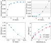 |
Fig. A.1. Fe K line properties of thermal emission spectrum. Top-left: Line centroid energy as a function of gas temperature; Top-right: Line intensity ratio of Fe XXVI and Fe XXV as a function of gas temperature. The dashed-line indicates the observed line ratio with 68% error region in grey shade; Bottom-left: Fe XXV EW as a function of temperature when the Solar metallity is assumed; and Bottom-right: Fe XXV EW as a function of metallicity for gas temperature of kT = 3 keV (blue) and kT = 5 keV (red). |
Appendix B: An unidentified 4.5 keV emission feature
There is a possible line-like excess at 4.5 keV in the total diffuse emission spectrum. The Ca K band spectrum at ∼4 keV indicates the temperature kT ∼ 1.8 keV (Fig. B.1). No emission-line feature is expected at 4.5 keV in a thermal emission spectrum of a similar temperature. We examined the 4.1-5 keV data for its detection with a power-law model with or without a narrow Gaussian line. The lower energy bound was chosen to avoid the Ca K emission. To optimise a line detection, we rebinned the data with 60-eV intervals, which samples the major part of a line feature by three bins at 4.5 keV, where the spectral resolution is FWHM ≃ 140 eV. The Gaussian centroid is found at 4.51 ± 0.03 keV. The line intensity is (7.8 ± 2.3)×10−7 ph cm−2 s−1, corresponding to a EW of 26 ± 8 eV. The continuum slope is α = 1.8 ± 0.3 when NH = 4 × 1022 cm−2 is assumed. We compared between the fits with and without the Gaussian line, using the Akaike Information Criterion (AIC) and Bayesian Information Criterion (BIC). The relative likelihood of the inclusion of the 4.5 keV line is 20 from BIC and 40 from AIC. The difference comes from the degree of penalisation on extra parameters. The detection of the line feature is reasonably strong. A possible identification is a neutral Ti K at 4.51 keV. The cold Fe K line at 6.4 keV is detected and might share the same origin. However, the 4.5 keV line is far too strong to match the cosmic abundance of Ti, which is ∼2 orders of magnitude smaller than Fe. Although the cosmic rays have much more elevated Ti abundance relative to Fe due to spallation, it is not relevant unless the line production is due to the charge exchange.
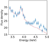 |
Fig. B.1. Diffuse emission spectrum of the central part of M82 in the 3.3-5 keV band. It illustrates the excess emission at 4.5 keV. The red histogram indicates the best fitting apec model, which describes the Ca feature at 3.9 keV. No strong atomic line feature that corresponds to the 4.5 keV emission is expected. The flux density is in units of 10−14 erg s−1 cm−2 keV−1. |
Appendix C: Image of dX36 and dX37 region from no transient flaring intervals
The region segments dX36 and dX37 contain the transient sources Xp7 and Xp11, respectively. Xp7 exhibited flares during the first two observations in 1999, while Xp11 during the three observations in 2010 (see the Chandra observation log in Table 1). Fig. C.1 shows the 4-8 keV image of the region around the two transient sources, obtained from the full 13 exposures (in the left panel) and that of the same region from eight exposures in which neither of them were in the flaring states (in the right panel). No point-like excess is seen at the positions of the two sources in the image when they were in quiescence. This justifies the use of their quiescence data to study the diffuse emission properties in the segments dX36 and dX37.
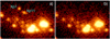 |
Fig. C.1. Comparison of the 4-8 keV images of the transient sources Xp7 and Xp11, taken from a) the total 13 exposures; and b) the eight exposures where both sources were in quiescence. The two transient sources are marked on the left panel. |
Appendix D: X-ray extinction map
The distribution of X-ray absorbing column density over the diffuse emission region is presented in Fig. D.1. The absorbing column density in each region-segment was obtained in two steps. The segment dX31 shows the least absorbed soft-band spectrum and fitting an absorbed apec model to the 0.9−1.7 keV spectrum gives a temperature of  keV, metallicity of
  and NH = 1.11(1.07 − 1.14)×1022 cm−2. Firstly, we fitted NH of the spectra of all the other segments in the same band, assuming the same temperature and metallicity. These NH are all in the range of (1 − 2)×1022 cm−2. They represent absorption for the soft X-ray wind and might not reflect the absorption towards the inner part where the hard X-ray emission comes from. All the spectra were fitted again but in the 4-7 keV band, assuming kT = 6 keV. When this hard-band NH exceeds that for the soft band, the hard-band NH was adopted. This applies to dX1, 14, 15, 18, 19, 26, 27, and 28, for which the 4-7 keV continua show a hard slope. It is found that a few regions show NH up to 1023 cm−2.
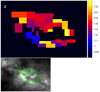 |
Fig. D.1. Extinction across the 4-8 keV diffuse emission region. a) X-ray absorbing column density, NH, map in units of 1022 cm−2. b) The R-band image of the central part of M82, taken by the Bok 2.3-m telescope at Kitt Peak National Observatory, overlaid by the 38 region segments where the X-ray absorbing columns were measured. |
For comparison, the optical image of the region taken in R band by the Bok 2.3-m telescope at Kitt Peak National Observatory, overlaid by the X-ray region segments, is also shown in Fig. D.1. The image was retrieved from NED. The region segments showing high NH values generally coincide with the dust lanes seen in the optical image.
Appendix E: Galactic centre positions
The positions of Xp9, radio source 43.21+61.3, the three kinematic centre measurements, the nuclear position measured by WISE (W1) in the WISE eXtended Source Catalogue (WXSC), and the two 2.2 μm peak measurements, plotted in Fig. 12, are reproduced in the Table below.
Galactic centre positions.
Appendix F: X-ray spectra of the diffuse emission from the 38 segments
 |
Fig. F.1. 0.7-7 keV Chandra spectra of the 38 region segments, dX0 through dX37, over the diffuse emission. The flux density, FE, is in units of 10−14 erg s−1 cm−2 keV−1. The two highest energy bins corresponds to the two Fe-line bands of cold Fe K at 6.4 keV and Fe XXV at 6.7 keV. |
All Tables
All Figures
|
Fig. 1. Chandra X-ray images of the central part of M 82 integrated over the 13 observations. Top left: 2−4 keV image. Top right: 4−8 keV band. The colour scale of these two images is in logarithmic with the brightest point sources are saturated. Bottom left: The 4−6 keV image of the ellipse where the data of the diffuse emission spectrum were taken. The detected discrete sources were masked. The region where the brightest ULXs along with a few others are clustered is masked in a block. This image is in a linear scale as the dynamic range of the brightness is narrow: 1−19, as a result of the removal of discrete sources. Bottom right: The same image as top right overlaid by the ellipse and the 38 region segments for spatially resolved spectral study. |
| In the text | |
|
Fig. 2. Diffuse emission spectrum of the central part of M 82, obtained from the Chandra ACIS-S. The flux density is in units of 10−14 erg s−1 cm−2 keV−1. Upper panel: The 0.7−8 keV spectrum. Lower panel: The Fe K band spectrum of the same data. The three vertical dotted-lines indicates the expected centroid energies of 6.4 keV, 6.7 keV and 6.96 keV for cold Fe K, Fe XXV and Fe XXVI, respectively. The grey line indicates the fitted model of a power-law and three Gaussian lines. |
| In the text | |
|
Fig. 3. Temperature (kT), metallicity (Z) and absorbing column density (NH) obtained from fitting the apec to the individual line spectra. The NH for the Fe K band spectrum was assumed to be 4 × 1022 cm−2, approximately the middle value obtained for the Ca spectrum, as the energy range of the data is insensitive to NH < 1023 cm−2. |
| In the text | |
|
Fig. 4. Spatial variations of spectral properties over the hard-band diffuse emission. Left: Surface brightness (upper panel) in units of 10−15 erg s−1 cm−2 arcsec−2 and energy index of power-law continuum (lower panel) in the 4−6 keV band. Middle: Surface brightness of 6.67 keV Fe XXV emission in units of 10−9 ph cm−2 s−1 arcsec−2 and line EW in units of keV. Right: Surface brightness and line EW of 6.4 keV cold Fe K emission in the same units as the Fe XXV emission. |
| In the text | |
|
Fig. 5. Values of the respective region segments in each map in Fig. 4 are plotted. From top to bottom: surface brightness of the 4−6 keV continuum in units of 10−15 erg s−1 cm−2 arcsec−2; the 4−6 keV energy index, α; surface brightness of cold Fe (6.4 keV, in blue) and hot Fe (Fe XXV at 6.67 keV, in red) in units of 10−9 ph s−1 cm−2 arcsec−2; and EW of cold Fe (6.4 keV) and hot Fe (6.67 keV) in units of keV. |
| In the text | |
|
Fig. 6. Separate CDFs of the surface brightness of the 4−6 keV continuum, Fe XXV and cold Fe (from left to right) in the northern (N, blue circles) and southern (S, red triangles) parts with respect to the starburst disc plane. These plots were made, using 29 segments with the 4−6 keV surface brightness cut (see text). The 4−6 keV continuum surface brightness is in units of 10−15 erg s−1 cm−2 arcsec−2 while the Fe line surface brightness is in units of 10−8 ph s−1 cm−2 arcsec−2. |
| In the text | |
|
Fig. 7. Plot of EW (Fe XXV) against continuum slope α of the 38 region segments (in blue filled-squares). The three magenta diamonds indicate the points for the EW-binned spectra (Table 3), where EW value of each point is the median of EWs measured in the spectra that went into each bin. |
| In the text | |
|
Fig. 8. Spectral variations as a function of Fe XXV EW. Left: The broad band spectrum of dX37, integrated spectra of Fe XXV EW of EW ≥ 0.3 keV, 0.15–0.3 keV, and < 0.15 keV (‘high’, ‘medium’, and ‘low’ from top to bottom). Each spectra has been multiplied arbitrarily for displaying purpose. Right: The Fe K band data of the high, medium, and low spectra in the left panel. The flux density is in units of 10−14 erg s−1 cm−2 keV−1. |
| In the text | |
|
Fig. 9. Image of the 4−8 keV emission overlaid by the two strips along the major axis: ‘Disc’ and ‘N’, and the two strips along the minor axis: ‘Centre’ and ‘E’. |
| In the text | |
|
Fig. 10. Light distribution in the 4−8 keV band. (a) The 4−8 keV projected light profiles along the major axis taken from the strips shown in Fig. 9. (b) The profiles along the minor axis. (c) These two panels show the same profiles but standardised for a comparison of their shapes. (d) The 4−8 keV diffuse emission image, constructed by two-dimensional interpolation from the point source masked image. Each pixel has an ≈2 × 2 arcsec2 size and the colour bar indicates the brightness scale in units of counts per pixel. |
| In the text | |
|
Fig. 11. Diffuse X-ray, FIR, and radio image comparison. Left: The 4−8 keV Chandra image in grey-scale overlaid by the Herschel-PACS 70 μm FIR contours in magenta. Right: The PACS 70 μm image overlaid by VLA 3-cm continuum (Adebahr et al. 2013) contours in green. The beam sizes of the PACS and the VLA images are ∼5.5 arcsec and 7.6 × 7.3 arcsec, respectively. Both contours are drawn in seven levels divided in linear scale with the lowest contour corresponding to 10% of the peak brightness in the respective images. |
| In the text | |
|
Fig. 12. Ks band image of the M 82 nuclear peak emission obtained from 2MASS in grey scale (fainter emission is cut out), overplotted by positions of the X-ray source, Xp9 (white), radio source 43.21+61.3 (red; Rodriguez-Rico et al. 2004), H I kinematic centre (green; Weliachew et al. 1984), Ne II kinematic centre (blue; Achtermann & Lacy 1995), H92α ring centre (cyan; Rodriguez-Rico et al. 2004), WISE peak (yellow; Jarrett et al. 2019), and two previous 2.2 μm peak measurements (R80: Rieke et al. 1980; L90: Lester et al. 1990). The positional error is ∼0.5″ for each measurement, which is represented by the circle, apart from the 2.2 μm position of Rieke et al. (1980). The image orientation is north up, east to the left. |
| In the text | |
|
Fig. 13. C-statistic curve for the Fe metallicity of Th2 in the joint fit of the three EW-sliced spectra and dX37 spectrum with the three continuum component model. |
| In the text | |
|
Fig. 14. Same spectrum shown in Fig. 2 with the best estimate of the three continuum components, IC (blue), Th1 (purple) and Th2 (red) assuming the Fe metallicity of Th2 to be 3.8 Z⊙. Two additional lines at 4.5 keV and 6.4 keV are also plotted in dotted lines. The flux density is in units of 10−14 erg s−1 cm−2 keV−1. |
| In the text | |
|
Fig. 15. Fe XXV EW map overlaid by the Subaru-COMICS mid-IR [Ne II] contours. The colour bar shows the Fe XXV EW in keV. The white arrows indicates the three Fe XXV-enhanced regions I, II, and III, which appear to fill the chimneys and to be connected to the mid-IR knot ‘E1’ (Achtermann & Lacy 1995). The orange arrow indicates the chimney with an expanding bubble identified around the SNR 41.95+57.5 by Wills et al. (1999). The two region-segments dX34 and dX35, discussed in the text, are also indicated. |
| In the text | |
|
Fig. 16. JVLA map at 3 GHz overlaid by the Subaru-COMICS [NII] contours. Three (or four) ‘wisps’ are seen both in mid-IR and radio on the northern side. The green diamond indicates the radio source, 43.21+61.3 of Rodriguez-Rico et al. (2004), which coincides with the X-ray source, Xp9, at the position of the radio kinematic centre. The five brightest radio SNRs, all of which have X-ray counterparts, are encircled in white. The radio SNR 41.95+57.5 (=X-ray SNR, Xp15) and presently the brightest radio SNR of SN2008iz (Brunthaler et al. 2009) are indicated. |
| In the text | |
|
Fig. 17. Spectral energy distribution of Xp9. The radio data points are from Rodriguez-Rico et al. (2004). The mid-IR data points are upper limits obtained from the Subaru-COMICS images (Gandhi et al. 2011). The luminosity range at 12 μm, expected from the low-luminosity AGN hypothesis, is indicated by the dotted-line, which could be within the reach of the upcoming JWST observations. |
| In the text | |
|
Fig. A.1. Fe K line properties of thermal emission spectrum. Top-left: Line centroid energy as a function of gas temperature; Top-right: Line intensity ratio of Fe XXVI and Fe XXV as a function of gas temperature. The dashed-line indicates the observed line ratio with 68% error region in grey shade; Bottom-left: Fe XXV EW as a function of temperature when the Solar metallity is assumed; and Bottom-right: Fe XXV EW as a function of metallicity for gas temperature of kT = 3 keV (blue) and kT = 5 keV (red). |
| In the text | |
|
Fig. B.1. Diffuse emission spectrum of the central part of M82 in the 3.3-5 keV band. It illustrates the excess emission at 4.5 keV. The red histogram indicates the best fitting apec model, which describes the Ca feature at 3.9 keV. No strong atomic line feature that corresponds to the 4.5 keV emission is expected. The flux density is in units of 10−14 erg s−1 cm−2 keV−1. |
| In the text | |
|
Fig. C.1. Comparison of the 4-8 keV images of the transient sources Xp7 and Xp11, taken from a) the total 13 exposures; and b) the eight exposures where both sources were in quiescence. The two transient sources are marked on the left panel. |
| In the text | |
|
Fig. D.1. Extinction across the 4-8 keV diffuse emission region. a) X-ray absorbing column density, NH, map in units of 1022 cm−2. b) The R-band image of the central part of M82, taken by the Bok 2.3-m telescope at Kitt Peak National Observatory, overlaid by the 38 region segments where the X-ray absorbing columns were measured. |
| In the text | |
|
Fig. F.1. 0.7-7 keV Chandra spectra of the 38 region segments, dX0 through dX37, over the diffuse emission. The flux density, FE, is in units of 10−14 erg s−1 cm−2 keV−1. The two highest energy bins corresponds to the two Fe-line bands of cold Fe K at 6.4 keV and Fe XXV at 6.7 keV. |
| In the text | |
Current usage metrics show cumulative count of Article Views (full-text article views including HTML views, PDF and ePub downloads, according to the available data) and Abstracts Views on Vision4Press platform.
Data correspond to usage on the plateform after 2015. The current usage metrics is available 48-96 hours after online publication and is updated daily on week days.
Initial download of the metrics may take a while.