| Issue |
A&A
Volume 673, May 2023
|
|
|---|---|---|
| Article Number | A136 | |
| Number of page(s) | 15 | |
| Section | Stellar structure and evolution | |
| DOI | https://doi.org/10.1051/0004-6361/202245468 | |
| Published online | 18 May 2023 | |
Expectations for fast radio bursts in neutron star–massive star binaries
1
ASTRON, the Netherlands Institute for Radio Astronomy, Oude Hoogeveensedijk 4, 7991 PD Dwingeloo, The Netherlands
e-mail: This email address is being protected from spambots. You need JavaScript enabled to view it.
2
Department of Physics, University of Warwick, Coventry CV4 7AL, UK
3
Astrophysics, Department of Physics, University of Oxford, Keble road Oxford OX1 3RH, UK
Received:
15
November
2022
Accepted:
29
March
2023
Abstract
Context. Recent observations of a small sample of repeating fast radio bursts (FRBs) have revealed a periodicity in their bursting activity that suggests a binary origin for the modulation.
Aims. We set out to explore the scenario where a subset of repeating FRBs originates in binary systems that host a highly energetic neutron star and a massive companion star, akin to γ-ray binaries and young high-mass X-ray binaries.
Methods. In this scenario, we infer observables, compare them with current observational constraints, and make predictions for future observations. Firstly, we specifically focused on the host galaxy properties and binary formation rates. Subsequently, we investigated the expected evolution of the rotation and dispersion measure in this scenario, the predicted birth site offsets, and the origin of the persistent radio emission observed in a subset of these systems.
Results. The host galaxies for repeating FRBs favour the formation of neutron star–massive star binary systems, but any conclusive evidence will require future discoveries and localisations of FRBs. The birth rate of high-mass X-ray binaries, used as a proxy for all considered binaries, significantly exceeds the estimated rate of FRBs, which can be explained if only a small subset of these systems produce FRBs. We show that, under simple assumptions, we can reproduce the dispersion measure and rotation measure evolution that is seen in a subset of repeating FRBs. We also discuss the possibility of detecting a persistent radio source associated with the FRB due to an intra-binary shock between the companion star wind and either the pulsar wind or giant magnetar flares. The observed long-term luminosity stability of the persistent radio sources is most consistent with a giant flare-powered scenario. However, this explanation is highly dependent on the magnetic field properties of the neutron star.
Conclusions. With these explorations, we provide a framework to discuss future FRB observations in the context of neutron star–massive star binary scenarios. We conclude that more localisations and observations of repeaters will be necessary to conclusively determine or rule out a connection between (repeating) FRBs and such binaries.
Key words: stars: neutron / stars: magnetars / X-rays: binaries
© The Authors 2023
 Open Access article, published by EDP Sciences, under the terms of the Creative Commons Attribution License (https://creativecommons.org/licenses/by/4.0), which permits unrestricted use, distribution, and reproduction in any medium, provided the original work is properly cited.
This article is published in open access under the Subscribe to Open model. This email address is being protected from spambots. You need JavaScript enabled to view it. to support open access publication.
1. Introduction
The discovery of fast radio bursts (FRBs), millisecond-duration radio flashes of cosmological nature, was a transformative event in the field of transient radio astronomy. To date, more than a decade after their discovery, more than 600 FRBs have been detected and reported, of which roughly 50 are known to repeat and 19 have associated host galaxies (see Petroff et al. 2022; The CHIME/FRB Collaboration 2023, for more details and references). Repeating FRBs are particularly vital to study their still poorly understood origin, as follow-up observations can enable the localisation, host galaxy identification, and searches for (multi-wavelength) persistent counterparts (see Nicastro et al. 2021, and the references therein). This highlights the need to discover larger numbers of FRBs, both repeaters or non-repeaters, with (future) instruments capable of measuring accurate positions for single bursts.
This work is motivated by two recent major developments in FRB observations. Firstly, two repeating FRBs that show periodicity in their activity cycle have been discovered (Rajwade et al. 2020; CHIME/FRB Collaboration 2020): FRB 20121102A was observed to show activity windows with a ∼160 day periodicity, while FRB 180916.J0158+65 shows such windows with a ∼16 day periodicity. These results are consistent with a binary system origin for the FRB, where orbital motion modulates the observed burst rate (see e.g., Ioka & Zhang 2020, although see Beniamini et al. 2020, Zanazzi & Lai 2020, and Sridhar et al. 2021 for alternative, non-binary explanations). Secondly, the Galactic magnetar SGR J1935+2154 showed extremely bright (∼MegaJansky) radio bursts with associated high-energy flaring (Bochenek et al. 2020; CHIME/FRB Collaboration 2020). In fact, several radio bursts spanning eight orders of magnitude were emitted by the magnetar, suggestive of a link between the known neutron star population and FRBs.
These two independent findings − activity periodicities that may imply a binary nature of the FRB source and the magnetar connection − warrant a detailed examination of systems that combines both properties (see also e.g., Tendulkar et al. 2021) and leads to the question of how the properties of binary systems that host a magnetar, or more generally a neutron star, compare to known FRB properties. The notion that many known Galactic neutron stars reside in binary systems further motivates this approach, as the same may hold for any neutron star energetic enough to power an FRB.
In this paper we explore the properties of binaries that host a neutron star with those of known FRBs. We also explore several predictions for FRB observables in this scenario: the positions of these systems in their host galaxies, the evolution of the dispersion and rotation measure (DM and RM, respectively) with time, and the properties of their persistent (radio) counterparts. In this approach, we are agnostic with respect to the specific underlying FRB model: we only assume that the neutron star in the system is energetic enough to power it. We start in Sect. 2 with a brief overview of types of galactic binaries that host a neutron star and then focus more specifically on neutron star–massive star systems in the rest of this paper. Section 2 also sets out the approach and structure for the remainder of our exploration.
2. Setting the stage: A brief overview of neutron stars in binaries
Galactic binaries hosting a neutron star and a non-degenerate companion star span a wide range of types, varying in a number of properties. Firstly, the two binary companions may interact via a range of processes, such as accretion (i.e. X-ray binaries; Patruno & Watts 2021; Reig 2011, for low and high-mass X-ray binary reviews, respectively), shocks between the pulsar wind and other components of the system (e.g., stellar winds from the companion; Dubus 2013), or ablation of the non-degenerate star (i.e. spider pulsars; Roberts 2013). In detached systems, on the other hand, such interactions do not take place. Across the wide zoo of neutron stars in binaries, basic neutron star properties differ greatly, as do those of the stellar companion: particularly, spin, magnetic field strength, and age of the neutron star, and mass, radius, and evolutionary status of the companion. Finally, the properties of the binary orbit itself, such as period and eccentricity, systematically differ between classes of binaries and systems of different age.
Assuming that this Galactic population is representative of extragalactic populations, the two recent FRB discoveries introduced in the previous section rule out a significant subset of them as FRB sources. Restricting the systems to those consistent with a magnetar primary and with binary orbits in the range of 16–160 days, we are left with young systems: specifically, those hosting a young, energetic neutron star and a massive donor star1. Here, the young neutron star matches with the magnetar constraint, while the binary orbits imply massive star companions2.
In the Milky Way, two known classes of systems fit the description of binaries hosting a young neutron star and a massive star: high-mass X-ray binaries (HMXBs) and γ-ray binaries. The former are young systems that host strongly magnetised (B > 1012 G) but slowly spinning (P > 1 s) neutron stars (Staubert et al. 2019) accreting from a massive companion (OB supergiants or Be stars, typically) in an orbit with periods spanning from days to years (Reig 2011). The latter are similarly young systems, where the neutron star typically resides in an eccentric orbit around a massive star. While γ-ray binaries are sometimes classified as a subset of HMXBs, we distinguish them as no active accretion is thought to take place; instead their interaction takes the form of an orbitally-varying collision shock between the pulsar and stellar wind (Dubus 2013). The neutron star spin period, and derived dipolar magnetic field strength, are only known for three γ-ray binaries: PSR B1259-63 (Manchester et al. 1995), LS I +61° 303 (Weng et al. 2022), and PSR J2032+4127 (Abdo et al. 2009). The known γ-ray binaries also display orbital periods of similar order of magnitude as the two FRB activity periods. These γ-ray binaries furthermore show that, for orbital periods of the order of tens to hundreds of days, accretion does not necessarily take place, even in eccentric systems. Indeed, for the typical mass ratios implied in a neutron star–massive star binary (NMB), most massive stars will not fill their Roche lobe (Underhill et al. 1979). Therefore, depending on the combination of outflow and circumstellar disc properties of the massive star (e.g., Grundstrom & Gies 2006) and the eccentricity (Martin et al. 2009), some system will and others will not allow accretion to take place.
In the remainder of this paper we compare these NMBs to FRB sources. We also assess the effect that the presence of the massive star may have on FRB observables. As stated, we are agnostic regarding the exact FRB mechanism – importantly, we do not assume it requires a binary companion. Therefore, the discussion in the remainder of this paper may only apply to a subset of FRBs.
In Fig. 1 we show a schematic overview of the structure of this paper. In the next section we focus on comparisons: we specifically compare existing constraints on formation rates of NMBs with the rates of FRBs (Sect. 3.1), and compare host galaxy properties of localised FRBs with relations between NMBs and their host galaxy environment (Sect. 3.2). Subsequently, we turn to predictions of an NMB scenario: at what position are they born and how do these positions evolve over time (Sect. 4.1); how does the presence of the massive star affect the (time-evolution of the) RM and DM (Sect. 4.2); and what persistent radio source (PRS) properties may be expected (Sect. 4.3). Finally, in Sect. 5 we discuss caveats that are at odds with an NMB scenario, after which we conclude in Sect. 6.
 |
Fig. 1. Schematic overview of the topics addressed in this paper and their structure in the text. We discuss galaxy properties and formation rates of NMB-type FRB sources in Sect. 3. Subsequently, we discuss the expected kicks and offset, DM and RM evolution, and persistent radio sources in Sect. 4. The galaxy in the left panel is a gri composite from the Sloan Digital Sky Survey, adapted from Masters et al. (2019). The middle panel shows a schematic depiction of an NMB surrounded by expanding material, and the right panel shows two configurations of an NMB, i.e. non-accreting (left) and accreting (right). |
3. Comparisons: Formation rates and host galaxy properties
3.1. Formation rates
Here we first discuss constraints on formation rates of NMB systems and compare them with observed FRB rates. Generally, a stringent test of any progenitor model for FRBs is whether the birth rate of the proposed progenitor agrees with those observed rates. In the framework that we discuss here, the relevant observed FRB rate concerns their birth rate, inferred from observations, instead of the rate of bursts themselves, given that a subset of FRBs repeat.
Firstly, we can approach this question by focusing on the FRB source itself. As relevant in the scenario investigated here, we consider the FRB to be produced by a strongly magnetised neutron star (e.g., magnetars). For a Milky Way-like galaxy, we assume a the birth rate of magnetars of 2.2 × 10⁻³ yr−1, based on estimates for magnetar birth rates in our Galaxy by several authors (see e.g., Gill & Heyl 2007, and references therein). While we know that isolated magnetars have the ability to produce bright radio bursts (Bochenek et al. 2020; CHIME/FRB Collaboration 2020), we then have to correct this rate by the expected number of magnetars to be in a binary system with a high mass stellar companion. Very recently, Chrimes et al. (2022) have used binary population and spectral synthesis (BPASS) simulations to show that the number of magnetars that can be expected to be in binary systems in our Galaxy is anywhere between 5–10%. Hence, the expected number of magnetars to reside in bound binary systems ranges between 1.1–2.2 × 10⁻⁴ yr−1.
In order to estimate the fraction of bound systems with massive star companions, we estimate the fraction of bound systems with companion masses comparable to OB-type stars. Following the recent review of Offner et al. (2022), we can assume that, before the supernova creating the neutron star, the primary star follows an initial mass function with power −2.3, while the secondary’s mass function is uniform between zero and the primary mass. In that case, under the prior information that the primary star was a massive star (e.g., producing a compact object), the probability of the secondary also being a massive star is of the order of tens of per cent. The total birth rate is corrected by this fraction to compute the fraction of bound magnetar systems with massive companions. Finally, to account for the beaming of FRBs away from the observer, we assume a beaming fraction similar to the Galactic radio pulsars of 10% (Faucher-Giguère & Kaspi 2006) to keep our simulations simplistic. Then, the expected birth rate of FRB progenitors that reside in NMB systems and visible from Earth can only be expected to be of the order of ∼10−5–10−6 yr−1. We highlight that the birth rate would be even lower if beaming is stronger for FRBs but the current estimates are highly unconstrained as the physical emission mechanism for FRBs is still unclear. This is consistent with the lack of a confirmed magnetar in a binary system with a high-mass binary companion in our Galaxy.
We can alternatively approach this question from the angle of HMXB formation rates. HMXBs are, or course, just one of the types of NMB. However, HMXB formation rates are best constrained from models and observations amongst interacting types. There are no constraints on non-interacting NMBs, making any estimates for these systems implausible. Hence, we first focus on the HMXB subset of NMBs for this comparison. Modelling of the Galactic HMXB population by Iben (1995) derived a formation rate of HMXBs of the order 2.6 × 10⁻³ yr−1, significantly larger than the above rate for magnetars with massive companions. Not all those HMXBs will necessarily host a neutron star primary. However, Iben (1995) note that the great majority of the modelled systems (≳84%) is expected to host a neutron star. Observationally, the Galactic population of HMXBs is indeed dominated by neutron star systems, of which a significant fraction hosts a Be-donor. Therefore, there is a more than two orders of magnitude discrepancy between the formation rate of Galactic neutron star HMXBs, and magnetars with high-mass donors. This discrepancy is increased further by accounting for the population of γ-ray binaries amongst NMBs, which are not included in the above rate estimates: Dubus et al. (2017) derive and expected number of  Galactic γ-ray binaries, which, despite its large uncertainties, would constitute a significant fraction of the number of NMBs. The rate discrepancy between these two lines of reasoning may be reconciled by the extreme nature of the neutron star required to produce the FRB (as well as, possibly, the PRS; see Sect. 4.3 with regards to the magnetic field and spin required in NMB scenarios for this persistent emission).
A low formation rate of energetic, fast-spinning magnetars in binaries is suggested by the lack of their detection in our Galaxy. Therefore, most of the formed NMBs may simply host a neutron star that is either never energetic enough to be the FRB source or only emits FRBs extremely rarely. In addition, orbital properties may reduce the discrepancy as well: for very short orbits, accretion may take place regularly, possibly suppressing neutron star – companion star interactions and magnetospheric FRB mechanisms; for wide-orbit systems, on the other hand, interactions between the two binary companions could become too weak to detect as a persistent source. Still, we can roughly estimate the upper limit on the fraction of NMBs that can host an FRB emitting magnetar to ≤1% based on the rate discrepancy. The fraction will be significantly lower if only a subset of magnetars are capable of producing FRBs. The current upper limit is consistent with the observed fraction of repeaters showing periodicity.
3.2. Galaxy properties of HMXB systems and FRB hosts
Building on the reasoning in the previous section, we can briefly turn our attention to the properties of the environment and host galaxy. The formation rate of NMBs, in relation to the properties of their environment, has been studied in particular for HMXBs, which we therefore focus on below. It is known to be heavily dependent on star formation rate (SFR) and metallicity (Dray 2006) of the galaxy. For instance, the formation rate of HMXBs has been constrained in the Large and Small Magellanic Clouds (LMC and SMC), which both underwent a burst of star formation in the last tens of megayears. For the SMC, Antoniou et al. (2010) infer a formation rate of 1 HMXB per 3 × 10⁻³ M⊙ yr−1 of star formation, during a period of star formation taking place between 25 and 60 Myr ago. The formation rate in the LMC was found to be approximately 17 times lower by Antoniou et al. (2010), at 1 system per 43.5 × 10⁻³ M⊙ yr−1 of star formation, dominated by a star formation burst 6–25 Myr ago. The difference between these rates has been attributed to metallicity, where the lower metallicity of the SMC leads to an increased formation of HMXBs per unit of SFR (for comparison, note that the Milky Way, which has a higher metallicity, hosts a factor of ∼50 fewer HMXBs per units stellar mass; Majid et al. 2004). At the same time, this lower metallicity also causes a higher fraction of systems hosting a Be-donor compared to OB supergiant donors, which may have effects on PRS scenarios (e.g., Sect. 4.3). Taking a complementary approach of considering X-ray luminosity functions (XLFs), the relation between the total number of HMXB in a galaxy and its global SFR has also been established by comparisons of galaxies spanning a range of ∼50 in SFR (Grimm et al. 2003; Gilfanov 2004): higher SFRs are found to be correlated with larger numbers of HMXBs (which dominate the XLF at high X-ray luminosities). The results suggest that, in an NMB model for FRBs, these FRBs should occur preferentially in high SFR and low metallicity environments.
More recent studies have shown that the relation between the number of HMXBs (or, more accurately, the XLF of a galaxy), the SFR, and the metallicity does not change in a detectable manner between redshifts z ∼ 0.1–2 (Douna et al. 2015; Fornasini et al. 2020; Lehmer et al. 2021) – a range overlapping with the redshifts of identified host galaxies of FRBs. Therefore, we can compare host galaxy SFRs and metallicities of localised FRBs, when known, with the empirically determined relation between SFR, [O/H], and XLF: log Lx ∝ β[O/H] × δ log SFR, where β = −0.91 ± 0.17 and δ = 1.06 ± 0.08 (Fornasini et al. 2020). In Fig. 2 we plot SFR versus 12+log(O/H) for the FRB host galaxies, while the background colour map traces the logarithm of the XLF, from low (light) to high (dark). The lines indicate contours in the XLF and increase by a factor of 10 between contours towards the bottom right. Finally, we include the Milky Way (based on Balser et al. 2011), LMC (Russell & Dopita 1992; Antoniou & Zezas 2016), and SMC (Russell & Dopita 1992; Antoniou et al. 2010) and show host galaxies of repeating FRBs in grey.
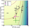 |
Fig. 2. SFR and metallicity of FRB hosts (non-repeaters shown with white-filled points, repeaters in grey), alongside the Milky Way, LMC, and SMC. The colour map shows the dependence of the XLF on SFR and metallicity on a logarithmic scaling, from low (top left, light colours) to high (bottom right, dark colours). The lines indicate XLF contours increasing in steps of a factor of 10, starting from an integrated X-ray luminosity of 1039 ergs s−1 for the top-left contour. The dark grey-filled point is FRB 20121102A. |
No clear trend is seen in the identified and characterised FRB hosts from Fig. 2, as was similarly noted in analyses by Heintz et al. (2020), Bhandari et al. (2020), and Li & Zhang (2020) in comparing the properties of host galaxies with other possible FRB progenitor types. It is, however, interesting to note that the host galaxy of FRB 20121102A (dark grey square) lies very close to the LMC and SMC, galaxies that show a larger population of NMBs. As larger numbers of FRB hosts are identified and characterised in the future, an NMB model would predict those to lie preferentially towards the bottom right of this diagram. However, as discussed in the previous section, the extreme nature of the neutron star that may be required to produce the FRB may be the dominant and limiting factor in whether a galaxy host an FRB source. Another aspect to take into account is the timescale on which the FRB-producing NMB evolves, compared to bursts of star formation: in the LMC and SMC, bursts of star formation tens of megayears ago are thought to be responsible for the current large populations of HMXB systems (Antoniou et al. 2010; Antoniou & Zezas 2016). Therefore, SFR estimates concurrent with FRB activity may not trace the presence of an FRB source, if the star formation activity lasted shorter than the lifetime of the massive binary before the first supernova (leading to the first of the FRB). However, those concerns may be more prominent for close-by systems such as the LMC and SMC, where burst of star formation may be spatially resolved, instead of galaxies where we consider the averaged properties of the system.
4. Predictions: Positions, DM and RM, and persistent radio sources
Having compared the formation rates and host galaxy properties of (subtypes of) NMBs to localised FRB hosts, we now turn to predictions in the NMB scenario. We focus these predictions on three themes, where recent observations have revealed interesting and surprising FRB behaviour: the positions of FRBs in their galaxy and compared to potential birth sites; the time evolution of their DM and RM; and the presence of persistent (multi-wavelength) emission. The recent results in each of these three provide a benchmark for our predictive discussion, while future studies of larger samples can test the expectations for NMBs.
4.1. Position and offsets and birth sites
Through the combination of accurate localisation and deep imaging of their host galaxy, the potential birth site of three FRBs has been determined: FRB 20121102A (Marcote et al. 2017), FRB 20180916B (Tendulkar et al. 2021), and FRB 20190520B (Niu et al. 2022). The possible offset between the FRB location and its birth place is consistent with a high peculiar motion of the FRB source, similar to Galactic compact objects (e.g., pulsar wind nebulae) and stars (e.g., runaway massive stars and hypervelocity stars). For an NMB system, such high velocities may be the result from the kick associated with the supernova that created the neutron star (e.g., Blaauw 1961), or with many-body interactions between the massive star(s) and other stars in its original massive star cluster (Poveda et al. 1967).
Using the observed proper motion properties of Galactic HMXBs, we can assess the positional offset distribution expected for an NMB-type FRB source. For this purpose, we perform population synthesis simulations of the motion of NMBs within their host galaxy. As our observational input is based primarily on Galactic HMXBs, we assume host galaxy properties similar to the Milky Way. While isolated pulsars are typically born with large kick velocities due to the violent way in which they are created (Hobbs et al. 2005), this does not apply for HMXBs: Bodaghee et al. (2021) found kick velocities for these systems in the range of 2–34 km s−1. These are the best kick constraints amongst the different types of NMBs and are the velocities projected over the sky plane (see Faucher-Giguère & Kaspi 2006, for more details). To account for the random direction of kick velocities in three dimensions, we draw the kick velocities from a zero-centred Gaussian distribution with a dispersion of 34 km s−1 over x, y and z-axis of the Cartesian co-ordinate system and then obtain the final velocity as a vector sum of the three components.
For each NMB, we then obtained its age by sampling from a uniform distribution between 0 and 10 Myr. In doing so, we assume that an NMB does not survive beyond 10 Myr, reflective of the timescale where the massive star is expected to end its life (we define that a binary becomes an NMB after the formation of a neutron star in the system). For the radial distribution of their original birth locations, we assume a distribution following the Galactic neutron star population (Yusifov & Küçük 2004) − effectively assuming that both pulsars and NMBs are correlated in similar fashion with star-forming region in our Galaxy. To simulate the time evolution of their positions, we then adopt an analytical model for the Galactic potential of the Milky Way: specifically, we adopt the modification by Kuijken & Gilmore (1989) of the Carlberg & Innanen (1987) fit of the Galactic gravitational potential. Thereby, we assume a combination of a disc-halo, bulge, and nucleus component, using the analytical forms and constants from Faucher-Giguère & Kaspi (2006).
Then, we evolved the NMBs as follows: (i) for each NMB, we assigned a birth velocity by drawing from the birth velocity distribution; (ii) we assigned an age by drawing from the uniform age distribution of NMBs; (iii) we assigned an initial birth position in the Galaxy by drawing from the radial and scale height distribution adopted from radio pulsars; and (iv) for a given birth velocity and initial position of the NMB, we evolved it through the Galactic potential for a duration equal to its age to get the final position in the Galaxy. For the purposes of these simulations and to get a statistically large sample of NMBs in the Galaxy, we simulated 200 systems using this method.
Finally, for each simulated NMB, we computed the offset from the birth site of the neutron star. To maximise the observed separation, we assumed a face-on orientation of the galaxy with respect to the observer. For an original NMB position X0, Y0 at the time of the birth of the neutron star and final position X1, Y1 in a galactocentric Cartesian co-ordinate system, the offset with respect to the observer is simply  parsec.
To show the results of this simulation, we present a histogram of resulting offsets in Fig. 3. The green curve indicates the histogram, while the three observed offsets, for FRB 20121102A, FRB 20180916B, and FRB 20190520B, are indicated by the vertical lines (converted from the observed angular offset between their assumed birth sites and their observed positions, using the host galaxy distance). We can see clearly how all three systems are consistent with the expected distribution for NMB type systems with typical Galactic kick velocities. We note that the age estimate we get for FRB 20121102A from the offsets is higher (∼106 yr) than what is postulated by other authors. One significant assumption in our estimate is that the offset measured for FRB 20121102A is from the centre of the star-forming region (Bassa et al. 2017), while the position of the FRB still lies within the half-light radius of the region. The inferred age will differ significantly depending the FRB source’s original location within the entire region; hence, our simulation does not rule other estimates invalid. We also note that there is an obvious observational bias in the measurement of offsets: systems with a smaller offset will be more straightforwardly associated with a star-forming region. The three localised FRBs where an offset has been measured make up only a small subset of all localised sources and may be biased towards smaller offsets.
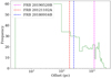 |
Fig. 3. Histogram of projected offset distribution for the simulations of NMB-FRBs as described in Sect. 4.1. The vertical lines show the offsets measured for the three well-localised repeating FRBs, indicating that they are consistent with the expected distribution in an NMB scenario. |
4.2. DM and RM evolution
Recent studies across time of several repeating FRBs have revealed variations in both the observed DM and RM, with significant variety in behaviour between sources. Monitored longest, FRB 20121102A can be characterised by the monotonic decrease in its RM over the span of 5–10 yr, while its DM gradually increased at a rate of ∼1 pc cm−3 yr−1 (Hilmarsson et al. 2021). On the other hand, FRB 20190520B has shown erratic variations in RM characterised by sign changes and large variations in magnitude (Anna-Thomas et al. 2022). Similarly, significant RM changes were observed in FRB 20201124A (Wang et al. 2022), while FRB 20180916B instead recently showed a secular rise in its RM (Mckinven et al. 2022). In an NMB-type scenario, both binary components can (indirectly) affect the RM and DM evolution with time: the remnant from the supernova that created the magnetar and the clumpy stellar wind from the massive companion star both supply ample material to interact with the FRB emission. While the former may naively be expected to cause a more gradual evolution over timescales of at least years, the latter may instead cause more erratic evolution on short timescales. In this section we explore the effects that both structures may have on the FRB’s RM and DM.
4.2.1. The effects of a supernova remnant
To assess the effects of a surrounding supernova remnant (SNR) on the time evolution of RM and DM, we assume a magnetar created in a supernova explosion starts emitting FRBs after a short time compared to the evolutionary timescales of the remnant. As the SNR expands and, at the same time, the NMB may move within, through, and then out of the SNR due to a supernova kick, significant RM and DM evolution may be expected. Previous works by Piro & Gaensler (2018) and Kundu (2022) have performed analyses of how the SNR should contribute to the DM and RM of the FRB with time. While we refer to those work for their detailed treatments, we instead formulate a similar analysis that makes simplifying assumptions while capturing the salient features of the SNR evolution. Our main aim is to investigate the expected DM and RM evolution on a macroscopic and qualitative level, but it should be noted that the final and exact qualitative contributions of the SNR to the DM and RM will depend on the ionisation fraction, ejected mass, NMB kick velocity, and the interstellar medium (ISM) composition (see Kundu 2022, for more details).
Specifically, we made the following assumptions for a SNR evolving in time. Firstly, we assumed that the SNR can be approximated as a spherically symmetric shell with a constant electron density within the shell surrounded by a thin layer of high-density swept-up material. For simplicity, we assumed that the shell is mostly made up of hydrogen and did not consider any heavier elements. Secondly, we assumed that a reverse shock is created as soon as the ejecta hits the surrounding ISM material (100 yr after the event), after which is takes of the order of ∼900 yr to propagate to the core of the remnant and ionise all the material within the shell (Micelotta et al. 2016). Until the time that reverse shocks reach the core and completely ionise the material within the shell, most of the material within the shell remains neutral (see Appendix A for more details about this assumption). Hence, we assumed an ionisation fraction of 10% until then. For this putative SNR, we used the measured values of various physical parameters based on the study by Micelotta et al. (2016) for Cas A, the best-studied Galactic SNR. We also evolved the ejecta velocity during different evolutionary stages – for example, the free expansion stage, the adiabatic stage (Sedov-Taylor), and the snow-plow phase – based on (Vink 2020) and Wang et al. (2015; see Appendix A for a detailed description of this calculation). Finally, we assumed the evolution of the magnetic field within the shell and at the shock front using the analytical treatment provided by Vink (2020). Using this framework, we evolved the motion of a compact object created in this remnant, as well as the structure of the remnant itself, assuming a range of kick velocities. Assuming two scenarios – a compact object either moving towards or away from the observer – we then estimated the expected changes in DM and RM over time.
In Fig. 4 we show the outcome of these calculations. In both columns, we show the DM (top), RM (middle), and SNR radius in comparison with NMB offset from the centre (bottom), all as a function of time since the supernova. The left column denotes the calculations assuming the NMB moves towards the observer; the right column assumes the NMB moves away from the observer. Different colours of the dashed lines indicate different NMB velocities, while the black dashed lines indicate the times when the SNR is assumed to transition between evolutionary stages.
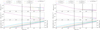 |
Fig. 4. DM and RM evolution of an NMB in a SNR. Left panel: three panels showing (from top to bottom) the DM, the RM, and the radius of the supernova shell as a function of time for a compact object moving towards the observer from the core of the shell with a certain radial velocity. The different colours denote the different radial velocities assumed for the compact object. The dashed vertical lines denote the times at which the ejecta velocity changes (corresponding to the evolutionary stage of the SNR). The dashed cyan line in the bottom panel shows the shell radius with time, and the other lines correspond to the object radius (distance of the compact object from the centre of the SNR). Right panel: same as the left panel but for the compact object moving away from the observer. |
Overall, we see that, when the NMB is moving towards the observer, the SNR expansion gradually causes a decay in both RM and DM over time. However, a clear drop in both, is predicted by the time the NMB leaves the SNR. For the case when the neutron star is moving away from the observer, the SNR expansion still causes a gradual decrease in RM and the DM. This can be attributed to the trade-off between the reduction in the electron density as the shell expands and the extra distance between the neutron star and the observer. In addition, once the NMB crosses the shell, more material intervenes the line of sight and an increase in both DM and RM is expected. This increase is, in a fractional sense, smaller than the decrease in the first scenario. We note how an arbitrary direction of the NMB between these two extremes will lead to an evolution in between both scenarios, with no sudden change in DM/RM expected at the shell-crossing for motions perpendicular to the line of sight.
This simplified calculation shows that one can replicate the DM and RM changes that are observed at least in some repeating FRBs. For example, the decrease in DM is fairly gradual during the last stage of evolution, which can be perceived as no detectable variability over a span of a few years, as seen for a few repeating FRBs (see e.g., Pleunis et al. 2021). Similarly, the RM contribution from the SNR decreases rapidly from being as high as 104 rad m−2 to barely observable within the first 1000 yr of the evolution. Rapid decreases in RM have indeed been observed for FRB 20121102A, while the RM of FRB 20180916B showed no variation over several years. Recently, however, its RM increased monotonically (Mckinven et al. 2022), which may be attributed to an NMB moving through the dense, magnetic shell of the SNR in a direction away from the observer. If these FRBs originate from an NMB inside a SNR, the DM and RM evolution in them could be used as a probe of the age of the system. We finally note that the variations in DM and RM from these calculations do not require the presence of a binary companion, but merely the presence of a compact object formed in the supernova. Therefore, they could be testable on repeaters that do not show any signature of orbital motion. However, the presence of massive binary companion will systematically decrease the velocity of the FRB emitter, delaying the onset of sudden changes in DM and RM.
4.2.2. The effects of clumpy massive star winds
The effects of the SNR are however, clearly, unable to reproduce the more erratic RM behaviour observed in FRB 20190520B and FRB 20201124A: large changes in the magnitude of the RM and, especially, sign reversals. Such effects do not show up in our calculations and appear problematic for this interpretation. Therefore, one can instead consider the additional effects of the strong wind of the massive star in an NMB on the RM (see also e.g., Wang et al. 2022): if this wind is clumpy, the line of sight may be crossed by a dense wind clump with a differently oriented magnetic field, leading to strong RM variations.
The variations in DM and RM in an NMB system due to the presence of a stellar wind, may be a combination of secular changes dependent on the orbital phase and the orbital orientation with respect to the observer, as well as stochastic changes set by the wind’s clumpy structure. Such DM and RM variations are indeed seen in studies of radio pulsars in eclipsing binaries and other γ-ray binary systems (Li et al. 2022). To calculate these effects on a potential FRB emitter in orbit around a massive star, we assume that this magnetar is close to periastron in its orbit, while traversing behind the massive companion. From observational and modelling studies, it is known that massive stellar winds may reach filling factors as high as 0.1 (Puls et al. 2006). To simulate such a clumpy wind, we first assume a baseline of a uniform wind where the electron density follows a radial profile of the type
 (1)
(1)
where n0 is the electron density close to the stellar surface, R0 is the stellar radius, and r is the distance from the star. We then added clumps stochastically with filling factors in the range of 0.1–0.01 onto that steady wind at different time intervals; those interval were chosen in a random manner under the assumption that the generation of clumps in the wind is a stochastic process best characterised by a Poisson distribution. Then, the DM along the line of sight is
 (2)
(2)
where RNS is the distance of the neutron star from the companion, Rout is the outer limit up to which the stellar wind contributes to the DM (∼100 stellar radii), and 𝒮(i, r, x) is the multiplicative factor that is required to convert the integral along our line of sight to a function of distance from the companion for an inclination angle (i) and the projected distance between the neutron star and the companion (x). Here, nclump is the electron density within the clump, N is the number of clumps, and l is the path length of the clump along our line of sight.
We finally assumed that magnetic field above the star evolves with distance as
 (3)
(3)
where B0 is the magnetic field close to the surface of the star. The clumps in the wind can induce magnetic fields that can have different directions, leading to variations in the RM due to the field reversals in the clumps. To account for these reversals, we randomly assign a sign to the magnetic field in each of the clumps. Similar to the DM, the RM contribution from the stellar wind is
 (4)
(4)
where Bclump is the magnetic field in the clump. The ± sign reflects the notion that the magnetic field component along our line of sight will have different signs for different clumps. We also ensure that the FRB is able to travel through this environment by computing the optical depth of the line of sight for the steady wind and the clumps. In order to do this, we compute the emission measure (EM) along with the DM for every line of sight (e.g., Wright & Barlow 1975). Then, assuming an electron temperature of 104 K for the wind and the clumps, we compute the opacity at 1.4 GHz (Draine 2011) and find τ ≪ 1, with values > 1 only when the neutron star is very close to being eclipsed by the companion. Assuming the velocity of the compact object along its orbit (i.e. compared to the stellar wind) to be 50 km s−1 for typical NMBs with orbital periods of a few years (Frank et al. 2002), we then simulated the DM and RM variations one measures as the object moves towards and away from the periastron. The nominal values for B0 and n0 and other parameters of the massive star are taken from Table 1 of Zhao et al. (2023). Figure 5 shows the secular changes combined with sudden rises and falls in the DM and RM values. If the inclination of the orbit is high, one can still see erratic change in RM without any discernible changes in DM similar to similar to FRB 20190520B (Wang et al. 2022; Anna-Thomas et al. 2022). The magnitude of change in RM and DM in the clumps is dependent on the filling factor of the clumps and will be larger for denser clumps. We also note that the average direction of the magnetic field can also flip if the massive star has a circum-stellar disc. The disc has a strong toroidal magnetic field that would manifest as a sign change in the RM as the neutron star passes through the different sides of the disc (Wang et al. 2022).
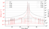 |
Fig. 5. DM and RM contribution from the clumpy stellar wind as the FRB progenitor moves behind the companion. The sudden changes in the DM and RM values are due to the clumps in the stellar wind. The vertical lines correspond to the jumps in DM and RM due to the clumps in the stellar wind. Different curves are shown for different inclinations of the orbit (0 corresponds to an edge-on orbit). The filling factor used for clumps for this simulation is 0.1. |
4.3. Persistent emission
In addition to detections of RM and DM variability, recent observations have also revealed PRSs associated with two repeating FRBs. With the exception of the Galactic source SGR 1935+2154, no persistent (or burst) counterparts have been identified at other wavelengths as of yet. In this section we compare known persistent radio emission mechanisms of Galactic NMBs to the observed FRB PRSs and discuss a possible alternative origin in the NMB scenario. Similar to Sect. 4.2, we also briefly mention the role that the SNR, expected around a young NMB, may play. However, we first summarise the relevant known observational properties of PRSs.
The PRS for FRB 20121102A was first detected, with a spectrum consistent with optically thin synchrotron emission and a specific luminosity of ∼2 × 1029 ergs s−1 Hz−1 (Marcote et al. 2017). More recent observations of this PRS by Plavin et al. (2022) reveal a compact source down to milliarcsecond scales, implying an intrinsic source size of < 1 pc. More recently, Niu et al. (2022) reported the identification of a PRS associated with FRB 20190520B, at a specific luminosity of 3 × 1029 ergs s−1 Hz−1. Not all searches reveal a PRS, however: Ravi et al. (2022) and Piro et al. (2021) report the detection of radio emission coincident with the position of FRB20201124A. However, both studies conclude that this emission likely originates from a star-forming region. Ravi et al. (2022) therefore place an upper limit on the PRS luminosity of 3 × 1028 ergs s−1 Hz−1. In this context, FRB20180916B is similarly noteworthy: no PRS is known, but Tendulkar et al. (2021) found the FRB to be offset by ∼250 parsec from a star-forming region where it may have originated between 800 kyr and 7 Myr ago.
The PRS of FRB 20121102A is best studied, especially across time due to its earliest discovery: upon its discovery, Chatterjee et al. (2017) report radio monitoring at 3 GHz across approximately two separate months, which are spaced out by approximately three months. This monitoring campaign does not show evidence for a systematic increase or decrease of the PRS radio luminosity, but does show apparently less-structured variability around its mean luminosity. Plavin et al. (2022) recently confirmed the absence of a luminosity decay on timescales of a year, which challenges several models for the nature of the PRS; particularly those invoking a transient radio counterpart powered by a single instance of energy injection (this possibility might still be feasible as we explain later). In the remainder of this section we use these basic observables – luminosities and (lack of) variability – to discuss the possibility of a PRS in the NMB scenario.
4.3.1. Basic considerations on the emission origin
We initially considered a number of possible emission origins before considering two options in more depth for the NMB scenario. Firstly, the transient radio emission from either a supernova or SNR, creating the FRB source, has been considered by various authors to model various aspects of the PRSs. Such scenarios are more general that the NMB case consider in this paper, but the neutron star in the NMB implies a supernova has taken place. Observationally, it is known that radio-detected supernovae typically rise in radio luminosity on timescales of days to hundreds of days, before subsequently decaying again. The radio-brightest examples peak at luminosities just above 1028 ergs s−1 Hz−1, roughly an order of magnitude below the two confirmed PRSs.
Recently, Eftekhari et al. (2019) reported the late-time radio brightening (after ∼7.5 yr) of the super-luminous supernova (SLSN) PTF10hgi, located at a redshift of z = 0.098. Its peak radio luminosity is similar to the radio-brightest other supernovae, around 1028 ergs s−1 Hz−1, again below that of PRSs. In addition, Hatsukade et al. (2021) report that in new observations, PTF10hgi has decreased in radio luminosity, suggesting its radio peak has occurred. Despite a number of searches across a range of timescales since the explosion, no other radio detections of SLSNe have been obtained (Mondal et al. 2020; Hatsukade et al. 2021; Eftekhari et al. 2021) – except for a handful of radio detections that are consistent with host galaxy radio emission. Several searches for FRBs from the positions of SLSNe have also failed to detect any (Law et al. 2019; Hilmarsson et al. 2021). While the transient nature of radio emission from SLSNe may also be challenging to reconcile with the stability of the FRB 20121102A PRS, a larger sample of radio-detected SLSNe would help in further assessing any possible connection.
Turning towards NMB-specific scenarios, a radio counterpart similar to those of Galactic HMXBs can be ruled out easily. Those accretion-driven radio sources (i.e. powered likely through the launch of relativistic jets from their accretion flow) have been shown to be order of magnitude radio fainter than PRSs (van den Eijnden et al. 2018, 2021). Even the handful of known, extreme, young X-ray binaries (such as Circinus X-1 or SS 433) do not reach the required luminosities in a sustained fashion; furthermore, the nature of their compact object remains unclear but is highly unlikely to be similar to the magnetar invoked for the NMB scenario. Finally, Sridhar & Metzger (2022) argue that radio nebulae created by the feedback of such extreme X-ray binaries would require mass accretion rates far exceeding those seen in the extreme Galactic X-ray binaries.
In our Galaxy, γ-ray binary systems are known to be radio-variable and bright systems. Their radio emission is not thought to be accretion driven, but instead shock driven: likely through shocks between the pulsar wind and stellar wind or decretion disc of their massive Be companion star (see Dubus 2013, for an extensive review). This motivates us to further explore the role such shocks may play in explaining PRSs, particularly for systems hosting young and extremely energetic magnetars – transporting the required energy via either their pulsar winds or giant magnetar flares. We note briefly that recently, scenarios involving a pulsar wind nebula (also referred to as a plerion) have been invoked as the explanation for the PRS (e.g., Murase et al. 2016; Kashiyama & Murase 2017; Chen et al. 2022). While we do not explore this here in detail, as it does not require a binary companion, it similarly poses that pulsar spin-down energy in converted to radio emission in shocks. However, those shocks then take place in the ISM instead, and could therefore be seen as a complementary option to our further discussion.
4.3.2. Persistent luminosities of shocks powered by spin-down or giant flares
Here, we first consider the energetics and time-averaged power budget of particle-accelerating intra-binary shocks, powered either by magnetar spin-down or giant flares. Starting with the former, we can consider the shocks taking place between pulsar wind and stellar wind or decretion disks, emitting non-thermally radio to very-high energy γ-rays (Dubus 2013). The emission is these systems is therefore thought to be powered, fundamentally, by the spin-down energy of the neutron star. The physical sizes of the resolved radio emitting regions in γ-ray binaries are of the order ∼120 AU (Moldón et al. 2011), significantly smaller than size upper limits of FRB PRSs. Their radio spectra are optically thin synchrotron spectra, consistent in spectral index with constraints in PRSs. An obvious discrepancy arises, however, when comparing the typical luminosities of both systems: γ-ray binaries are, at their brightest, several order of magnitude radio fainter than detected PRSs. Galactic γ-ray binaries are likely significantly older sources than FRB PRSs: PSR B1259-63, for instance, has a spin-down age of 330 kyr and an inferred bipolar magnetic field strengths of B ≈ 3.3 × 10¹¹ G. Therefore, we can explore a scenario whether a very young, rapidly spinning magnetar in a γ-ray-binary-like configuration may power an FRB PRS.
Initially ignoring time variability (see Sect. 4.3.3), the typical radio luminosity of PSR B1259-63 is approximately 6 × 1029 erg s−1 at 2 GHz, or 3 × 10²⁰ ergs s−1 Hz−1 (Dubus 2013). Of all γ-ray binaries, its spin-down energy is constrained best, at ∼8 × 1035 erg s−1 (Manchester et al. 1995)3. For comparison, the PRS of FRB 20121102A instead has a specific radio luminosity approximately 9 orders of magnitude higher, and would therefore require a spin-down energy of the order of ∼8 × 1044 erg s−1 if we assume the same efficiency between spin-down power and radio luminosity of the inter-binary shock. Such a spin-down energy upper limit can only be feasible if a millisecond magnetar is formed in the system: for a magnetic field of B = 1014 G, it would require a spin frequency ν > 211 Hz. On the other hand, assuming the pulsar spin does not exceed ∼2 × 10³ Hz, the magnetic field should exceed at least ∼1012 G. Such magnetars have been proposed as progenitors of repeating FRBs (see e.g., Margalit & Metzger 2018). While this scenario is extreme, we note that the 156.9-day activity cycle in FRB 20121102A is significantly shorter than the 1236 day orbital period in PSR B1259-63. As the shock power decreases with stand-off distance from the pulsar, ∼8 × 1044 erg s−1 could be considered an upper limit in this interpretation; the actual value could feasibly be (more than) an order of magnitude lower.
Since γ-ray binary shocks emit across the entire electromagnetic spectrum, we should also consider whether detectable high energy emission may be expected in this scenario. In the X-ray band, we can again scale up Galactic γ-ray binaries for this comparison. Scaling the typical X-ray flux of PRS B1259-63 to the distance of FRB 20121102A, while also including the ∼9 orders of magnitude higher normalisation due to the extreme required spin-down energy, one may expect expect a ∼10−14 erg s−1 cm−2 X-ray flux for FRB 20121102A in this γ-ray binary scenario. This value slightly exceeds the X-ray upper limit from (Scholz et al. 2017), although this can be reconciled if the interstellar absorption ∼3 times higher then assumed when deriving that upper limit (which remains consistent with the NH – DM relation from He et al. 2013). Furthermore, the X-ray to radio luminosity ratio of PSR B1259-63 is significantly higher than for other γ-ray binaries. At their lower ratios, the X-ray flux of FRB 20121102A would indeed fall far below the observed limit. This effect may strongly depend on the orbital separation, which affects the X-ray/radio ratio of the intra-binary shock. However, deep X-ray observations with future, low-background X-ray observatories could provide better X-ray tests of this shock scenario.
At current γ-ray sensitivities and, especially, angular resolutions, the detection of an extragalactic persistent γ-ray counterpart is not expected. While the emission of Galactic γ-ray binaries peaks at a few hundred MeV, it is limited by the pulsar spin-down energy, and this γ-ray flux varies along the binary orbit. In the above scenario, therefore, the expected time-averaged γ-ray flux remains undetectable in, for example, Fermi/LAT surveys. In addition, the relatively low angular resolution of γ-ray instruments challenges the confident identification of a persistent counterpart; indeed, as of yet, no constraining γ-ray limits on persistent emission have been reported.
A possible effect in this intra-binary shock scenario may be ablation effects of the massive companion star. Ablation is known to take place in spider pulsars, where a very-low-mass companion of a millisecond pulsar is slowly stripped of its outer layers by the energetic pulsar wind. A millisecond magnetar with an extreme spin-down energy may similarly ablate and strip a massive donor star. Following the formalism proposed by Ginzburg & Quataert (2020, 2021), one can derive that such a spin-down power greatly reduces the timescales of effective ablation. While important differences exist between spider pulsars and NMBs – the massive star is expected to reside more deeply within its Roche lobe and launches its own wind that shocks and balances the pulsar wind – these ablation effects pose a challenge for spin-down-powered PRS scenarios.
Instead of pulsar spin-down, the intra-binary shock may alternatively be magnetically powered, via the equivalent of a giant magnetar flare. The large amount of energy released in such a giant flare could lead to a PRS, as the highly energetic accelerated particles encounter the massive star’s stellar wind. In an intra-binary shock between this wind of energetic particles and the stellar wind, synchrotron emission may arise as particles are trapped by and then gyrate in the wind’s magnetic field. For instance, the Galactic magnetar SGR 1806-20 emitted a giant flare that injected ∼1046 ergs of energy into its environment (Palmer et al. 2005). A radio afterglow was also detected after this event that showed re-brightening over the timescale of days (Gelfand et al. 2005). While the radio luminosity of the afterglow is again orders of magnitude lower than typical PRSs, one can explore a scenario where a PRS is powered for a longer period of time from a giant flare from a magnetar with a much larger magnetic field. While the radio afterglow in SGR 1806-20 was likely caused by shocks in swept-up ambient material, the presence of a massive star and its wind also provide a denser medium for the formation of such shocks.
To consider more quantitatively whether the PRS can be powered by magnetar flares, we here make the assumption that the total energy emitted during a giant flare is proportional to the square of the magnetic field. The aforementioned Galactic magnetar SGR 1806-20, which emitted the 1046 erg giant flare, has an estimated magnetic field of ∼1014 G. We then assume that flare-induced shock is powered by the interaction between the magnetar wind emitted during the flare and the stellar wind of the massive companion. The particles in the resulting shock are not expected to diffuse out quickly, as they are confined by the stellar wind’s magnetic field. As a consistency check, we computed the Larmor radius of the electrons for typical values of the Lorentz factor (10–1000). The Larmor radius is  m where mc2 is the rest mass in the units of GeV, vsp is the velocity perpendicular to the magnetic field, q is the charge is units of the elementary change and B is the magnetic field in Tesla. For electrons with GeV energies, the Larmor radius is 3.3 × 10⁵vsp km. For large speeds (0.1–0.5c), we obtain Larmor radius of ∼10 000 km. This is much smaller than the typical length-scale of a flare interaction with the stellar wind, thus enabling particle confinement.
The typical synchrotron cooling timescale of particles,  s where, γ0 is the Lorentz factor and B is magnetic field at the interaction location. For relativistic particles (i.e. those that will emit broad-band synchrotron emission in the radio band), γ0 ∼ 102 and for τ ≥ 103 yr, B ≤ 10−4 G. For electrons with GeV energies, This value is consistent with the expected wind magnetic field at the location of the interaction (Walder et al. 2012). Hence, the shock will emit its energy budget at a relatively constant radio luminosity over its lifetime, instead of evolving significantly on the synchrotron cooling timescale. We can use this approach to scale the emitted energy for a range of magnetic fields of the neutron star. Assuming either a 1% or 0.01% efficiency of conversion to radio emission during the interaction with the stellar wind, we can compute the luminosity of the PRS for a range of survival times of the PRS (note that the lifetime does not equal the age of the system but instead to total time the PRS is active). Figure 6 shows the results of such an analysis. We can see that in this case, an extremely large magnetic field is required (1016 G) to power a PRS for a few hundred years at their observed luminosities. This again suggests that only FRB progenitors that are young will be able to power a PRS at the luminosity comparable to the PRS of FRB 20121102A.
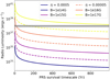 |
Fig. 6. Radio luminosity of the PRS as a function of the lifetime of the PRS, assuming no time evolution of the radio luminosity, for the case where a magnetar giant flare powers a PRS from the interaction with the stellar wind of the companion. Solid and dashed lines correspond to different efficiencies of conversion to radio emission (0.05 and 0.005%, respectively), and different sets of lines correspond to different surface magnetic fields of the neutron star, as shown in the legend. The horizontal grey region indicates the observed PRS luminosity of FRB 20121102A taken from Chen et al. (2022). |
While the population of accelerated particles, trapped in the stellar wind’s magnetic field, will also emit a higher energies, such an X-ray or γ-ray counterpart will be short lived and therefore challenging to detect. Synchrotron cooling, for instance, scales inversely with the square root of the characteristic emission frequency. Therefore, if the radio-emitting population survives for 103 yr, the X-ray counterpart will fade on a timescale of ∼10 days. The γ-ray counterpart will be even shorter lived. As these transient counterparts are not associated with a specific radio burst, randomly catching them is unlikely, in particular in source where a PRS is already detected. Furthermore, if other processes (e.g., inverse Compton cooling from interactions with stellar photons) speeds up the cooling, a high-energy counterpart detection is even less likely. A counterpart would similarly be expected at frequencies in between the radio and X-ray band, with an increasing lifetime towards lower frequencies.
4.3.3. The time evolution of NMB shock models
While the previous section focuses broadly on luminosity arguments, we should also incorporate the constraints on radio variability of PRSs obtained over the past five years. For the PRS of FRB 20121102A, for instance, apparently stochastic variability was observed (Chatterjee et al. 2017). However, no systematic decrease of its radio luminosity has been identified over a timescale of several years: it appears variable around a relatively stable specific luminosity of 2 × 1029 ergs s−1 Hz−1. Therefore, the NMB scenarios described above, should be able to explain such a stable luminosity with superimposed variations. Here, we assess how the luminosity of an intra-binary shock, powered by a magnetar giant flare or by spin-down, would evolve with time.
The spin-down-powered intra-binary shock scenario for an NMB, as well as the supernova scenario, are depicted schematically in Fig. 7. The main panel of this figure shows the evolution of the radio luminosity of different sources as a function time. The circles show data from the relativistic supernovae SN2008bb (Soderberg et al. 2010, red) and SN2012ap (Margutti et al. 2014; Chakraborti et al. 2015, green), as well as the late-time re-brightening of the SLSN PTF10hgi (Eftekhari et al. 2019). The light blue shaded region schematically depicts the region covered by current detections of Type Ic supernovae. Finally, the blue dashed line shows the radio luminosity of the PRS of FRB 20121102A, where we plot a constant value as no systematic, long-term radio evolution has been measured. As we do not expect strong time-evolution on the shown timescales for the giant-flare-powered scenario (by definition in the calculation; see above), we have not included this in the figure.
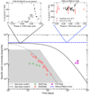 |
Fig. 7. Schematic overview of the time evolution of the radio luminosity of several discussed scenarios for the PRS. Note that the spin-down models represent the orbitally averaged luminosity and do not show the expected orbital modulation; this modulation is shown in the insets. The grey region indicates the typical region where type Ic supernovae are observed. See Sect. 4.3.3 for details. |
The dotted and full black lines show the γ-ray binary type scenario, where the dipolar spin-down powers the radio emission at a constant efficiency. As detailed in Appendix B, we plot the time evolution due to the decrease in spin-down energy, assuming an initial magnetic field of either 3 × 10¹² G (case I) or 1014 G (case II) and a initial spin required to match the PRS radio (i.e. following the same scaling calculation as in the previous section). In both cases, time evolution is still expected on the timescale of several years, inconsistent with available PRS observations. This may imply that an even higher magnetic field may be required, which increases the duration of the initial luminosity plateau visible for case II; however, more likely, it indicates how the dipolar spin-down is too simplistic an assumption to model the time evolution for these extreme systems; therefore, magnetar flares may instead be a more favourable power source.
As stated, initial radio observing campaigns of FRB 20121102A also revealed seemingly stochastic variability around its typical radio luminosity. On the top right panel of Fig. 7, we show the observations by Chatterjee et al. (2017) and Plavin et al. (2022) of the PRS of FRB 20121102AA, rescaled to 1.7 GHz using a spectral index α = −0.54 and folded on the period of its FRB activity cycle (156.9 days). In the NMB scenario, the activity cycle represents the binary orbit, on which intra-binary shocks are expected to be variable: γ-ray binaries are known to be variable along their orbit, as well as unrelated to orbital phase (see e.g., the example of the radio monitoring of the γ-ray binary PSR B1259-63 around periastron plotted in the top left panel of Fig. 7, adapted from Johnston et al. 1999). Similarly, in colliding wind binaries, where synchrotron-emitting shocks arise between two massive star winds, strong orbital variability is observed due to variation in distance between the stars. For the NMB case, particularly of a spin-down-powered shock, distance variations along an eccentric orbit could similarly lead to variability, as periodically a larger and smaller fraction of pulsar wind is traversing and powering the shock. In the currently published observations of the PRS of FRB 20121102A, we do not distinguish clear variability on the activity cycle timescale. However, these observations either suffer from low signal-to-noise (red points) or cover only part of a single orbit (black points). Therefore, we propose that detailed and systematic radio monitoring across activity windows is required to fully study the unexplained PRS variability of FRB 20121102A.
In the NMB scenario, PRS time evolution is automatically tied to spatial movement and therefore also to RM and DM variability. The PRS, in both intra-binary shock scenarios, would move with the FRB source as the entire binary travels from its birth place. In the spin-down-powered case, the long-term decrease in radio brightness would, eventually, render the PRS undetectable: indeed, FRB 20180916B may have travelled ∼250 pc over > 800 kyr to reach its current position (Tendulkar et al. 2021) and does not have an associated PRS at the level of FRB 20121102A and FRB 20190520B. The position of the PRS of 20121102A, on the other hand, remains within the half-light radius of its probable natal star-forming region (at current positional accuracy Marcote et al. 2017). This consistency implies a relatively young age (< 5.8 Myr assuming a velocity of 34 km s−1), fitting in the above scenario. If the intra-binary shock is instead powered by giant magnetar flares, the PRS may be expected to remain detectable on longer timescales (tens of kiloyears).
If the intra-binary shock PRS is only detectable at relatively young ages, its detection should be associated with high, fast-evolving RM and DM since the system remains embedded in the SNR. If repeating bursts are a signature of a young FRB source, one would expect to find a detectable PRS only for repeating sources (i.e. due to a physical reason instead of an observational bias driven by the localisations of repeaters). However, inversely, a young source does not necessarily imply a detectable PRS: for both intra-binary shock scenarios, the radio luminosity depends too strongly on the natal properties of the pulsar, as well as orbital properties such as eccentricity and separation, to always render a detectable persistent counterpart. Such differences may also manifest as differences in radio variability between PRSs, either in the decrease versus time or orbitally superimposed – therefore, FRB 20190520B may show different time evolution than FRB 20121102A does, in the NMB scenario.
From these comparisons, we conclude that the physical size limits, specific luminosity and a lack of high-energy counterpart to FRB PRSs may be explained in an NMB scenario. In that case, the PRS would be more likely powered by giant magnetar flares than pulsar spin-down, given the lack of observed decrease in PRS luminosity on timescales of years. Orbital variations of the radio luminosity may instead be expected on the timescale of the FRB activity cycle, which future observational campaigns may attempt to detect. Similarly, deep X-ray observations with future observatories may search for high-energy counterparts of the radio-emitting shocks. This scenario also predicts that PRSs are only detectable for young FRB sources. We do note the important caveat that intra-binary shocks will be highly dependent on the properties of the binary – therefore, the inferences drawn here from FRB 20121102A may not be representative of the entire population.
5. Discussion
While the FRB observables discussed in the previous two sections may be explained to certain extent in an NMB scenario, we briefly discuss a couple of further limitations and caveats here, while also proposing a handful of future observables that may test or rule out an NMB scenario.
Firstly, in our considerations, we have assumed the host galaxy properties to be similar to the Milky Way. While hosts of repeating FRBs have different morphologies, SFRs, and physical sizes compared to the Milky Way, the expected NMB distribution and density in the Milky Way (based on the X-ray luminosity as a proxy for HMXBs) is consistent with the properties of host galaxies of the published repeating FRBs (see Fig. 2). Therefore, we believe that assuming a Milky Way like host to perform our simulations is a reasonable assumption.
Recently, Pastor-Marazuela et al. (2021) showed that for FRB 20180916B, the burst activity window is frequency dependent: bursts at lower observing frequencies appear earlier than those at high frequency, while lasting for a longer duration as well (see also Pleunis et al. 2021). These results suggest that if the FRBs are produced in the magnetosphere of the compact object, they will be affected by the intra-binary medium of the binary system that will completely contradict the observed chromaticity in FRB 20180916B. However, we do note that these observations do not completely rule out the binary scenario. Very recently, Li et al. (2021) have introduced a model where FRBs are generated by a neutron star in a Be X-ray binary system, claiming that accretion induces star-quakes on the neutron surface resulting in FRBs. Their simulations have already shown that free-free absorption from the circum-stellar disc can mimic the chromatic burst activity of FRB 20180916B without invoking a non-binary model. Furthermore, several authors have also suggested binary models that can explain the low frequency activity of FRB 20180916B (see Deng et al. 2021, and the references therein).
The recent localisation of the repeating FRB 20200120E to a globular cluster in M81 (Kirsten et al. 2021) is very challenging to incorporate into an NMB scenario. While any magnetar-based FRB model will require an exotic formation channel to explain the presence of a magnetar in such an old population, the presence of massive binary companion is unlikely – whether in a natal binary system or through dynamical capture. In any FRB mechanism that requires the presence of a binary companion, such as the ones discussed in the previous paragraph, the globular cluster localisation of FRB 20200120E implies different mechanisms across the FRB population. In that case, no PRS would be expected for FRB 20200120E through the mechanisms considered in Sect. 4.3; in other words, if a PRS of FRB 20200120E is detected with similar properties to the other PRSs, it argues against the interpretation presented in Sect. 4.3 and an NMB model. Similarly, our discussions of the RM and DM variations (Sect. 4.2) requires that FRB 20200120E not show similar variability. If the origin of FRB activity windows is related to the binary period, FRB 20200120E should also not show such periodicity in its activity. Observations so far have not revealed a periodicity in this repeating FRB (Nimmo et al. 2023).
More generally than just for FRB 20200120E, the evolution of the RM and DM in repeaters is a testable prediction for the NMB scenario: a periodic variation will be seen in the RM and DM variation that is correlated with the burst activity window. We do note that the detectable modulation in the DM and RM with orbital phase is very much dependent on the orbital inclination angle and hence may not be true for all repeating FRBs (Pleunis et al. 2021). Furthermore, if the orbits are circular, we do not expect any variation in the DM and RM due to the orbit. Similar tests can be performed with the time-dependent evolution of the PRS, which is expected to be irregular or orbital on short timescales but decaying on longer (i.e. a large number of orbits) timescales as the magnetar spins down. Finally, if a close-by repeater is localised, we may expect to detect an optical persistent counterpart in the form of the massive OB companion star. If, on the other hand, the increase in the number of localised FRBs shows that a substantial fraction of them reside in globular clusters, an NMB scenario for FRBs will become less likely.
6. Conclusions
In this paper we critically examine a scenario where an FRB progenitor is a neutron star in a binary orbit around a massive star (referred to as an NMB system). We discuss the expectations of such a scenario for different properties of repeating FRBs, such as the offsets from the birth sites of the FRB progenitors (assuming that the FRB progenitor is a highly energetic neutron star), the evolution of RM and DM as a function of time, or the existence of a PRS in such systems.
Firstly, we considered the expected birth rates of HMXBs, as a proxy for NMBs, in comparison with FRBs and conclude that the discrepancy between the two can be reconciled if a very small subset of NMBs host a neutron star capable of producing FRBs. We report an upper limit to this fraction of 1% that is consistent with the current observations and expected rates of young, energetic neutron stars in our Galaxy. We also investigated any potential correlations between host galaxy properties of well-localised repeaters and galaxy properties that dictate the formation of NMBs. We show that current repeater hosts all fall in the region of galaxies expected to host a larger population of NMBs, although the results remain inconclusive at this point due to low number statistics.
Using simple models, we then discuss how such a population of NMBs can mimic the offsets from star-forming regions seen for a few repeaters, as well as the observed RM and DM evolution for repeating FRBs; the large diversity seen in the RM and DM variations of known repeaters may, in this scenario, be explained by the stellar wind of a massive companion star. Finally, we comment on the potential for detecting a PRS in an NMB. We considered several possibilities and come to the conclusion that the PRS could be produced by an intra-binary shock with the massive star’s wind, powered by the neutron star’s spin-down or giant magnetar flares. We find that the observed stability of PRS emission over timescales of years fits best with the latter power source.
With these discussions, we have aimed to provide a framework to discuss future FRB observations in the context of NMB-type scenarios. In conjunction, we currently conclude that larger numbers of localisations and observations of repeaters will be necessary to conclusively determine or rule out a connection between (repeating) FRBs and NMBs.
We discuss the recent localisation of an FRB in a globular cluster, i.e. an old population, in Sect. 5.
Note that this introduces an observational bias: non-interactive systems with a wide orbit and a low-mass companion may exist but would not be observed as binaries. However, as we discuss in Sect. 4.3, a massive companion star may help explain the presence of PRSs at FRB positions.
A spin measurement was recently reported for the γ-ray binary LS I +61° 303 (Weng et al. 2022). However, no spin derivative has been measured yet.
Acknowledgments
The authors thank the anonymous reviewer whose comments significantly improved the manuscript. The authors thank Jason Hessels and Joeri van Leeuwen for helpful comments on a draft version of this work. KMR would like to thank Zorawar Wadiasingh for useful discussions. KMR acknowledges funding from the European Research Council (ERC) under the European Union’s Horizon 2020 research and innovation programme (grant agreement No 694745). KMR acknowledges support from the Vici research programme “ARGO” with project number 639.043.815, financed by the Dutch Research Council (NWO). JvdE is supported by a Lee Hysan Junior Research Fellowship awarded by St. Hilda’s College, Oxford. We gratefully acknowledge support from the Leids Kerkhoven-Bosscha Fonds (LKBF). The research leading to these results has received funding from the European Union’s Horizon 2020 Programme under the AHEAD2020 project (grant agreement n. 871158).
References
- Abdo, A. A., Ackermann, M., Ajello, M., et al. 2009, Science, 325, 840 [Google Scholar]
- Anna-Thomas, R., Connor, L., Burke-Spolaor, S., et al. 2022, ArXiv e-prints [arXiv:2202.11112] [Google Scholar]
- Antoniou, V., & Zezas, A. 2016, MNRAS, 459, 528 [Google Scholar]
- Antoniou, V., Zezas, A., Hatzidimitriou, D., & Kalogera, V. 2010, ApJ, 716, L140 [NASA ADS] [CrossRef] [Google Scholar]
- Balser, D. S., Rood, R. T., Bania, T. M., & Anderson, L. D. 2011, ApJ, 738, 27 [NASA ADS] [CrossRef] [Google Scholar]
- Bassa, C. G., Tendulkar, S. P., Adams, E. A. K., et al. 2017, ApJ, 843, L8 [NASA ADS] [CrossRef] [Google Scholar]
- Beniamini, P., Wadiasingh, Z., & Metzger, B. D. 2020, MNRAS, 496, 3390 [NASA ADS] [CrossRef] [Google Scholar]
- Bhandari, S., Sadler, E. M., Prochaska, J. X., et al. 2020, ApJ, 895, L37 [NASA ADS] [CrossRef] [Google Scholar]
- Blaauw, A. 1961, Bull. Astron. Inst. Neth., 15, 265 [NASA ADS] [Google Scholar]
- Bochenek, C. D., Ravi, V., Belov, K. V., et al. 2020, Nature, 587, 59 [NASA ADS] [CrossRef] [Google Scholar]
- Bodaghee, A., Antoniou, V., Zezas, A., et al. 2021, ApJ, 919, 81 [NASA ADS] [CrossRef] [Google Scholar]
- Carlberg, R. G., & Innanen, K. A. 1987, AJ, 94, 666 [NASA ADS] [CrossRef] [Google Scholar]
- Chakraborti, S., Soderberg, A., Chomiuk, L., et al. 2015, ApJ, 805, 187 [NASA ADS] [CrossRef] [Google Scholar]
- Chatterjee, S., Law, C. J., Wharton, R. S., et al. 2017, Nature, 541, 58 [NASA ADS] [CrossRef] [Google Scholar]
- Chen, G., Ravi, V., & Hallinan, G. W. 2022, ApJ, submitted [arXiv:2201.00999] [Google Scholar]
- CHIME/FRB Collaboration (Andersen, B. C., et al.) 2020, Nature, 587, 54 [Google Scholar]
- Chrimes, A. A., Levan, A. J., Fruchter, A. S., et al. 2022, MNRAS, 513, 3550 [NASA ADS] [CrossRef] [Google Scholar]
- Crawford, I. A., Craig, N., & Welsh, B. Y. 1997, A&A, 317, 889 [NASA ADS] [Google Scholar]
- Deng, C.-M., Zhong, S.-Q., & Dai, Z.-G. 2021, ApJ, 922, 98 [NASA ADS] [CrossRef] [Google Scholar]
- Douna, V. M., Pellizza, L. J., Mirabel, I. F., & Pedrosa, S. E. 2015, A&A, 579, A44 [NASA ADS] [CrossRef] [EDP Sciences] [Google Scholar]
- Draine, B. T. 2011, Physics of the Interstellar and Intergalactic Medium (Princeton University Press) [Google Scholar]
- Dray, L. M. 2006, MNRAS, 370, 2079 [NASA ADS] [CrossRef] [Google Scholar]
- Dubus, G. 2013, A&A Rev., 21, 64 [NASA ADS] [CrossRef] [Google Scholar]
- Dubus, G., Guillard, N., Petrucci, P.-O., & Martin, P. 2017, A&A, 608, A59 [NASA ADS] [CrossRef] [EDP Sciences] [Google Scholar]
- Eftekhari, T., Berger, E., Margalit, B., et al. 2019, ApJ, 876, L10 [NASA ADS] [CrossRef] [Google Scholar]
- Eftekhari, T., Margalit, B., Omand, C. M. B., et al. 2021, ApJ, 912, 21 [NASA ADS] [CrossRef] [Google Scholar]
- Faucher-Giguère, C.-A., & Kaspi, V. M. 2006, ApJ, 643, 332 [CrossRef] [Google Scholar]
- Fornasini, F. M., Civano, F., & Suh, H. 2020, MNRAS, 495, 771 [NASA ADS] [CrossRef] [Google Scholar]
- Frank, J., King, A., & Raine, D. J. 2002, Accretion Power in Astrophysics: Third Edition, (Cambridge, UK: Cambridge University Press) [Google Scholar]
- Gelfand, J. D., Lyubarsky, Y. E., Eichler, D., et al. 2005, ApJ, 634, L89 [NASA ADS] [CrossRef] [Google Scholar]
- Gilfanov, M. 2004, MNRAS, 349, 146 [NASA ADS] [CrossRef] [Google Scholar]
- Gill, R., & Heyl, J. 2007, MNRAS, 381, 52 [NASA ADS] [CrossRef] [Google Scholar]
- Ginzburg, S., & Quataert, E. 2020, MNRAS, 495, 3656 [Google Scholar]
- Ginzburg, S., & Quataert, E. 2021, MNRAS, 500, 1592 [Google Scholar]
- Grimm, H. J., Gilfanov, M., & Sunyaev, R. 2003, MNRAS, 339, 793 [Google Scholar]
- Grundstrom, E. D., & Gies, D. R. 2006, ApJ, 651, L53 [NASA ADS] [CrossRef] [Google Scholar]
- Hamilton, A. J. S., & Sarazin, C. L. 1984, ApJ, 287, 282 [NASA ADS] [CrossRef] [Google Scholar]
- Hatsukade, B., Tominaga, N., Morokuma, T., et al. 2021, ApJ, 911, L1 [NASA ADS] [CrossRef] [Google Scholar]
- He, C., Ng, C. Y., & Kaspi, V. M. 2013, ApJ, 768, 64 [NASA ADS] [CrossRef] [Google Scholar]
- Heintz, K. E., Prochaska, J. X., Simha, S., et al. 2020, ApJ, 903, 152 [NASA ADS] [CrossRef] [Google Scholar]
- Hilmarsson, G. H., Michilli, D., Spitler, L. G., et al. 2021, ApJ, 908, L10 [NASA ADS] [CrossRef] [Google Scholar]
- Hobbs, G., Lorimer, D. R., Lyne, A. G., & Kramer, M. 2005, MNRAS, 360, 974 [Google Scholar]
- Iben, Icko Jr., & Tutukov, A. V., & Yungelson, L. R., 1995, ApJS, 100, 217 [NASA ADS] [CrossRef] [Google Scholar]
- Ioka, K., & Zhang, B. 2020, ApJ, 893, L26 [NASA ADS] [CrossRef] [Google Scholar]
- Johnston, S., Manchester, R. N., McConnell, D., & Campbell-Wilson, D. 1999, MNRAS, 302, 277 [NASA ADS] [CrossRef] [Google Scholar]
- Kashiyama, K., & Murase, K. 2017, ApJ, 839, L3 [NASA ADS] [CrossRef] [Google Scholar]
- Kirsten, F., Snelders, M. P., Jenkins, M., et al. 2021, Nat. Astron., 5, 414 [Google Scholar]
- Kuijken, K., & Gilmore, G. 1989, MNRAS, 239, 605 [Google Scholar]
- Kundu, E. 2022, MNRAS, 512, L1 [NASA ADS] [CrossRef] [Google Scholar]
- Law, C. J., Omand, C. M. B., Kashiyama, K., et al. 2019, ApJ, 886, 24 [NASA ADS] [CrossRef] [Google Scholar]
- Lehmer, B. D., Eufrasio, R. T., Basu-Zych, A., et al. 2021, ApJ, 907, 17 [NASA ADS] [CrossRef] [Google Scholar]
- Li, Y., & Zhang, B. 2020, ApJ, 899, L6 [NASA ADS] [CrossRef] [Google Scholar]
- Li, Q.-C., Yang, Y.-P., Wang, F. Y., et al. 2021, ApJ, 918, L5 [NASA ADS] [CrossRef] [Google Scholar]
- Li, D., Bilous, A., Ransom, S., Main, R., & Yang, Y. P. 2022, ArXiv e-prints [arXiv:2205.07917] [Google Scholar]
- Majid, W. A., Lamb, R. C., & Macomb, D. J. 2004, ApJ, 609, 133 [NASA ADS] [CrossRef] [Google Scholar]
- Manchester, R. N., Johnston, S., Lyne, A. G., et al. 1995, ApJ, 445, L137 [NASA ADS] [CrossRef] [Google Scholar]
- Marcote, B., Paragi, Z., Hessels, J. W. T., et al. 2017, ApJ, 834, L8 [CrossRef] [Google Scholar]
- Margalit, B., & Metzger, B. D. 2018, ApJ, 868, L4 [NASA ADS] [CrossRef] [Google Scholar]
- Margutti, R., Milisavljevic, D., Soderberg, A. M., et al. 2014, ApJ, 797, 107 [NASA ADS] [CrossRef] [Google Scholar]
- Martin, R. G., Tout, C. A., & Pringle, J. E. 2009, MNRAS, 397, 1563 [CrossRef] [Google Scholar]
- Masters, K. L., Lintott, C. J., Hart, R. E., et al. 2019, MNRAS, 487, 1808 [NASA ADS] [CrossRef] [Google Scholar]
- Mckinven, R., Gaensler, B. M., Michilli, D., et al. 2022, ArXiv e-prints [arXiv:2205.09221] [Google Scholar]
- Micelotta, E. R., Dwek, E., & Slavin, J. D. 2016, A&A, 590, A65 [NASA ADS] [CrossRef] [EDP Sciences] [Google Scholar]
- Moldón, J., Johnston, S., Ribó, M., Paredes, J. M., & Deller, A. T. 2011, ApJ, 732, L10 [CrossRef] [Google Scholar]
- Mondal, S., Bera, A., Chandra, P., & Das, B. 2020, MNRAS, 498, 3863 [NASA ADS] [CrossRef] [Google Scholar]
- Murase, K., Kashiyama, K., & Mészáros, P. 2016, MNRAS, 461, 1498 [NASA ADS] [CrossRef] [Google Scholar]
- Nicastro, L., Guidorzi, C., Palazzi, E., et al. 2021, Universe, 7, 76 [NASA ADS] [CrossRef] [Google Scholar]
- Nimmo, K., Hessels, J. W. T., Snelders, M. P., et al. 2023, MNRAS, 520, 2281 [NASA ADS] [CrossRef] [Google Scholar]
- Niu, C. H., Aggarwal, K., Li, D., et al. 2022, Nature, 606, 873 [NASA ADS] [CrossRef] [Google Scholar]
- Offner, S. S. R., Moe, M., Kratter, K. M., et al. 2022, Protostars and Planets VII, ed. Shu-ichiro Inutsuka, Yuri Aikawa, Takayuki Muto, Kengo Tomida, and Motohide Tamura [Google Scholar]
- Palmer, D. M., Barthelmy, S., Gehrels, N., et al. 2005, Nature, 434, 1107 [NASA ADS] [CrossRef] [Google Scholar]
- Pastor-Marazuela, I., Connor, L., van Leeuwen, J., et al. 2021, Nature, 596, 505 [NASA ADS] [CrossRef] [Google Scholar]
- Patruno, A., & Watts, A. L. 2021, Astrophys. Space Sci. Lib., 461, 143 [NASA ADS] [CrossRef] [Google Scholar]
- Petroff, E., Hessels, J. W. T., & Lorimer, D. R. 2022, A&A Rev., 30, 2 [NASA ADS] [CrossRef] [Google Scholar]
- Piro, A. L., & Gaensler, B. M. 2018, ApJ, 861, 150 [NASA ADS] [CrossRef] [Google Scholar]
- Piro, L., Bruni, G., Troja, E., et al. 2021, A&A, 656, L15 [NASA ADS] [CrossRef] [EDP Sciences] [Google Scholar]
- Plavin, A., Paragi, Z., Marcote, B., et al. 2022, MNRAS, 511, 6033 [NASA ADS] [CrossRef] [Google Scholar]
- Pleunis, Z., Michilli, D., Bassa, C. G., et al. 2021, ApJ, 911, L3 [NASA ADS] [CrossRef] [Google Scholar]
- Poveda, A., Ruiz, J., & Allen, C. 1967, Boletin de los Observatorios Tonantzintla y Tacubaya, 4, 86 [Google Scholar]
- Puls, J., Markova, N., Scuderi, S., et al. 2006, A&A, 454, 625 [NASA ADS] [CrossRef] [EDP Sciences] [Google Scholar]
- Rajwade, K. M., Mickaliger, M. B., Stappers, B. W., et al. 2020, MNRAS, 495, 3551 [NASA ADS] [CrossRef] [Google Scholar]
- Ravi, V., Law, C. J., Li, D., et al. 2022, MNRAS, 513, 982 [CrossRef] [Google Scholar]
- Reig, P. 2011, Ap&SS, 332, 1 [Google Scholar]
- Roberts, M. S. E. 2013, in Neutron Stars and Pulsars: Challenges and Opportunities after 80 years, ed. J. van Leeuwen, 291, 127 [Google Scholar]
- Russell, S. C., & Dopita, M. A. 1992, ApJ, 384, 508 [NASA ADS] [CrossRef] [Google Scholar]
- Scholz, P., Bogdanov, S., Hessels, J. W. T., et al. 2017, ApJ, 846, 80 [NASA ADS] [CrossRef] [Google Scholar]
- Soderberg, A. M., Chakraborti, S., Pignata, G., et al. 2010, Nature, 463, 513 [NASA ADS] [CrossRef] [Google Scholar]
- Sridhar, N., & Metzger, B. D. 2022, ApJ, 937, 5 [NASA ADS] [CrossRef] [Google Scholar]
- Sridhar, N., Metzger, B. D., Beniamini, P., et al. 2021, ApJ, 917, 13 [NASA ADS] [CrossRef] [Google Scholar]
- Staubert, R., Trümper, J., Kendziorra, E., et al. 2019, A&A, 622, A61 [NASA ADS] [CrossRef] [EDP Sciences] [Google Scholar]
- Tendulkar, S. P., Gil de Paz, A., Kirichenko, A. Y., et al. 2021, ApJ, 908, L12 [CrossRef] [Google Scholar]
- The CHIME/FRB Collaboration (Andersen, B. C., et al.) 2023, ApJ, 947, 83 [NASA ADS] [CrossRef] [Google Scholar]
- Underhill, A. B., Divan, L., Prevot-Burnichon, M. L., & Doazan, V. 1979, MNRAS, 189, 601 [CrossRef] [Google Scholar]
- van den Eijnden, J., Degenaar, N., Russell, T. D., et al. 2018, Nature, 562, 233 [NASA ADS] [CrossRef] [Google Scholar]
- van den Eijnden, J., Degenaar, N., Russell, T. D., et al. 2021, MNRAS, 507, 3899 [NASA ADS] [CrossRef] [Google Scholar]
- Vink, J. 2020, Physics and Evolution of Supernova Remnants (Springer International Publishing) [CrossRef] [Google Scholar]
- Walder, R., Folini, D., & Meynet, G. 2012, Space Sci. Rev., 166, 145 [NASA ADS] [CrossRef] [Google Scholar]
- Wang, F. Y., Zhang, G. Q., Dai, Z. G., & Cheng, K. S. 2022, Nat. Commun., 13, 4382 [NASA ADS] [CrossRef] [Google Scholar]
- Wang, L., Cui, X., Zhu, H., & Tian, W. 2015, in AdvancingAstrophysics with the Square Kilometre Array (AASKA14), 64 [Google Scholar]
- Weng, S.-S., Qian, L., Wang, B.-J., et al. 2022, Nat. Astron., 6, 698 [NASA ADS] [CrossRef] [Google Scholar]
- Wright, A. E., & Barlow, M. J. 1975, MNRAS, 170, 41 [Google Scholar]
- Yusifov, I., & Küçük, I. 2004, A&A, 422, 545 [NASA ADS] [CrossRef] [EDP Sciences] [Google Scholar]
- Zanazzi, J. J., & Lai, D. 2020, ApJ, 892, L15 [NASA ADS] [CrossRef] [Google Scholar]
- Zhao, Z. Y., Zhang, G. Q., Wang, F. Y., & Dai, Z. G. 2023, ApJ, 942, 102 [NASA ADS] [CrossRef] [Google Scholar]
Appendix A: Assumptions for the calculation of DM and RM in a SNR shell
A.1. Ionisation fraction
We assumed that supernova ejecta form a shell of uniform density with a thicker layer of swept-up material on the edge of the shell. The remnant is assumed to be predominantly made up of hydrogen. We consider four main stages of the supernova evolution: (i) free expansion phase; (ii) adiabatic phase (Sedov-Taylor); (iii) radiative phase (snowplough); and (iv) dispersion phase. For the free expansion phase, we assumed that the reverse shock was created ∼100 years after the event and takes about 900 years to reach the newly formed compact object. This is assuming a forward shock velocity of 5226 km s−1 and a reverse shock velocity of 1700 km s−1 (Micelotta et al. 2016). During the early stages of the free expansion stage, the recombination rate for singly ionised atoms is typically high (∼10−12 cm−3 s−1), so the rate becomes comparable to the ionisation rate at the time
 (A.1)
(A.1)
where Ai is the mean atomic weight, ne is the electron density, ni is the ion density, α is the recombination rate, Mej is the ejecta mass and vej is the ejecta velocity. For any time t > trec, the effects of recombination on the ionisation fraction of the ejecta are significantly reduced. However, by that time, the photon radiation field is weak enough that most of the ejecta tends to be neutral. Once the reverse shock is created, it propagates through the ejecta and the ejecta is optically thick to the photoionizing radiation of the reverse shock until the time
 (A.2)
(A.2)
where aν is the photoionisation cross-section (Draine 2011). For our case, using numbers for Cas A from Micelotta et al. (2016) and assuming the ne=ni for hydrogen, we estimate trec and topt of 15 and 922 years, respectively. This suggests that the ejecta is mostly neutral until the reverse shock reaches the core and completely ionises the ejecta within the shell. A detailed treatment of the evolution of the ionisation fraction is beyond the scope of this paper and hence we assume a fraction of 10% until the reverse shock reaches the core of the remnant. These equations and assumptions are adopted from Hamilton & Sarazin (1984).
A.2. Velocity of the ejecta
We assumed a different velocity evolution for the different phases of the supernova. During the free expansion phase, we assume the velocity to be completely constant at 5226 km s−1. This assumption holds true until the swept-up mass becomes equal to the ejecta mass, which happens around t∼700-1000 years for type-II supernovae (Draine 2011). During the adiabatic phase, the swept up mass is much larger than the ejecta mass, causing the ejecta to decelerate. Sedov (1959) provides a solution for this phase such that the shock pressure is proportional to the ideal gas pressure of the monoatomic gas. Hence, the velocity of the ejecta is
 (A.3)
(A.3)
where E* is the total energy released in the supernova event, ρ0 is the mass density of the ejecta, and Rs is the radius of the shell. We used Eq. A.3 to evolve the supernova shell from t = 103 to t = 2.5 × 10⁴ years. For the radiative phase, we can use conservation of momentum of the shell to get the velocity of the shell at any time, t,
 (A.4)
(A.4)
where V0 is the downstream velocity, R0 is the shell radius. The velocity evolves in this way from t = 2.5 × 10⁴ to t = 106 years. In the dispersion phase, we assume that the velocity of ejecta is almost equal to the velocity in the circumstellar medium (10 km s−1; Crawford et al. 1997).
A.3. Magnetic field
The magnetic field evolution in a SNR can be parametrised as
 (A.5)
(A.5)
where Vs is the shock velocity, ρ0 is the mass density of the material and x parameterises the relationship between the magnetic field and the properties of the shock (temperature, pressure, density etc.). Typically, the density profile of the ejecta follows  where Rs is the shock radius and s=−2. The radius roughly evolves as tm where m = 1.0. Hence,
 (A.6)
(A.6)
where B0 is the magnetic field at time t0. the values for B0 and t0 were again adopted from Micelotta et al. (2016) for Cas A. We assume x = 1.0 and use this equation to evolve the magnetic field in the SNR with time. The detailed mathematical derivations of the equations, as well as the values of different parameters presented here, are provided and discussed in Vink (2020).
A.4. Simulations
For the final simulations, we split the time from 0 to 5 × 10⁶ years into steps of 10 years. In order to compute the electron density, we assume the number density and the forward shock radius for Cas A from Table 1 from Micelotta et al. (2016). Then, under the assumption that the entire shell was ionised and had this uniform density, we compute the total number of electrons within the shell. We use this number them to compute the electron density for any time step in our simulation depending on the radius of the shell at that time step. For each time step, we compute the radius, the density, the magnetic field and the distance travelled by the neutron star based on its kick velocity. We then use those values to compute the DM and RM for that given time step as measured by the observer.
Appendix B: Time evolution of the spin-down-powered model
To calculate the time evolution of the spin-down-powered PRS luminosity, we assume for simplicity a dipole model where  ; when C0 = 3.2 × 10¹⁹ G/
 , the magnetic field is given in units of G. Assuming negligible changes in magnetic field strength, the spin period will evolve as
  , where P0 is the initial spin period. The aforementioned relation between the spin, spin-down, and magnetic field then yields the time-dependent spin-down rate; combined, we can estimate the time evolution of the spin-down energy as − Ė = 4π2IṖ(t)/P(t)3, where I is the pulsar’s moment of inertia. Finally, the spin-down energy is converted to radio luminosity assuming the same, constant efficiency as PSR B1259-63 (Johnston et al. 1999), for which a spin-down energy of 8 × 1035 erg/s yields a specific radio luminosity of 3 × 10²⁰ erg/s/Hz.
All Figures
|
Fig. 1. Schematic overview of the topics addressed in this paper and their structure in the text. We discuss galaxy properties and formation rates of NMB-type FRB sources in Sect. 3. Subsequently, we discuss the expected kicks and offset, DM and RM evolution, and persistent radio sources in Sect. 4. The galaxy in the left panel is a gri composite from the Sloan Digital Sky Survey, adapted from Masters et al. (2019). The middle panel shows a schematic depiction of an NMB surrounded by expanding material, and the right panel shows two configurations of an NMB, i.e. non-accreting (left) and accreting (right). |
| In the text | |
|
Fig. 2. SFR and metallicity of FRB hosts (non-repeaters shown with white-filled points, repeaters in grey), alongside the Milky Way, LMC, and SMC. The colour map shows the dependence of the XLF on SFR and metallicity on a logarithmic scaling, from low (top left, light colours) to high (bottom right, dark colours). The lines indicate XLF contours increasing in steps of a factor of 10, starting from an integrated X-ray luminosity of 1039 ergs s−1 for the top-left contour. The dark grey-filled point is FRB 20121102A. |
| In the text | |
|
Fig. 3. Histogram of projected offset distribution for the simulations of NMB-FRBs as described in Sect. 4.1. The vertical lines show the offsets measured for the three well-localised repeating FRBs, indicating that they are consistent with the expected distribution in an NMB scenario. |
| In the text | |
|
Fig. 4. DM and RM evolution of an NMB in a SNR. Left panel: three panels showing (from top to bottom) the DM, the RM, and the radius of the supernova shell as a function of time for a compact object moving towards the observer from the core of the shell with a certain radial velocity. The different colours denote the different radial velocities assumed for the compact object. The dashed vertical lines denote the times at which the ejecta velocity changes (corresponding to the evolutionary stage of the SNR). The dashed cyan line in the bottom panel shows the shell radius with time, and the other lines correspond to the object radius (distance of the compact object from the centre of the SNR). Right panel: same as the left panel but for the compact object moving away from the observer. |
| In the text | |
|
Fig. 5. DM and RM contribution from the clumpy stellar wind as the FRB progenitor moves behind the companion. The sudden changes in the DM and RM values are due to the clumps in the stellar wind. The vertical lines correspond to the jumps in DM and RM due to the clumps in the stellar wind. Different curves are shown for different inclinations of the orbit (0 corresponds to an edge-on orbit). The filling factor used for clumps for this simulation is 0.1. |
| In the text | |
|
Fig. 6. Radio luminosity of the PRS as a function of the lifetime of the PRS, assuming no time evolution of the radio luminosity, for the case where a magnetar giant flare powers a PRS from the interaction with the stellar wind of the companion. Solid and dashed lines correspond to different efficiencies of conversion to radio emission (0.05 and 0.005%, respectively), and different sets of lines correspond to different surface magnetic fields of the neutron star, as shown in the legend. The horizontal grey region indicates the observed PRS luminosity of FRB 20121102A taken from Chen et al. (2022). |
| In the text | |
|
Fig. 7. Schematic overview of the time evolution of the radio luminosity of several discussed scenarios for the PRS. Note that the spin-down models represent the orbitally averaged luminosity and do not show the expected orbital modulation; this modulation is shown in the insets. The grey region indicates the typical region where type Ic supernovae are observed. See Sect. 4.3.3 for details. |
| In the text | |
Current usage metrics show cumulative count of Article Views (full-text article views including HTML views, PDF and ePub downloads, according to the available data) and Abstracts Views on Vision4Press platform.
Data correspond to usage on the plateform after 2015. The current usage metrics is available 48-96 hours after online publication and is updated daily on week days.
Initial download of the metrics may take a while.