| Issue |
A&A
Volume 675, July 2023
|
|
|---|---|---|
| Article Number | A175 | |
| Number of page(s) | 24 | |
| Section | Catalogs and data | |
| DOI | https://doi.org/10.1051/0004-6361/202245191 | |
| Published online | 18 July 2023 | |
Time-resolved spectral catalogue of INTEGRAL/SPI gamma-ray bursts
Max-Planck-Institut für extraterrestrische Physik,
Giessenbachstraße 1,
85748
Garching, Germany
e-mail: bbiltzing@mpe.mpg.de
Received:
12
October
2022
Accepted:
31
May
2023
Since its launch in 2002, the International Gamma-Ray Astrophysics Laboratory (INTEGRAL) satellite has detected many gamma-ray bursts (GRBs), which are summarised in the INTEGRAL Burst Alert System (IBAS) catalogue. This catalogue combines triggers from the data of the Imager on Board the INTEGRAL (IBIS) and of the anti-coincident shield (ACS) of the SPectrometer on INTEGRAL (SPI). Since the Germanium detectors of SPI also serve as a valuable GRB detector on their own, we present an up-to-date time-resolved catalogue covering all GRBs detected by SPI through the end of 2021 in this work. Thanks to SPI’s high energy coverage (20 keV−8 MeV) and excellent energy resolution, it can improve the modelling of the curvature of the spectrum around the peak and, consequently, it could provide clues on the still unknown emission mechanism of GRBs. We split the SPI light curves of the individual GRBs in time bins of approximately constant signals to determine the temporal evolution of spectral parameters. We tested both the empirical spectral models as well as a physical synchrotron spectral model against the data. For most GRBs, the SPI data cannot constrain the high-energy power law shape above the peak energy, but the parameter distributions for the cut-off power law fits are similar to those of the time-resolved catalogue of gamma-ray burst monitor (GBM) GRBs. We find that a physical synchrotron model can fit the SPI data of GRBs well. While checking against detections of other GRB instruments, we identified one new SPI GRB in the SPI field of view that had not been reported before.
Key words: gamma-ray burst: general / methods: data analysis / catalogs
© The Authors 2023
 Open Access article, published by EDP Sciences, under the terms of the Creative Commons Attribution License (https://creativecommons.org/licenses/by/4.0), which permits unrestricted use, distribution, and reproduction in any medium, provided the original work is properly cited.
This article is published in open access under the Subscribe to Open model.
Open Access funding provided by Max Planck Society.
1 Introduction
The International Gamma-Ray Astrophysics Laboratory (INTEGRAL) (Winkler et al. 2003) hosts a suite of instruments dedicated to the study of the high-energy Universe. One of those instruments is the SPectrometer on INTEGRAL (SPI). As an MeV imaging telescope, it covers an energy range from 20 keV to 8 MeV and one of its scientific objectives is the detection, localisation, and study of gamma-ray bursts (GRBs; Vedrenne et al. 2003). There have been many studies of GRBs with SPI since the launch of INTEGRAL (Malaguti et al. 2003; Mereghetti et al. 2003; von Kienlin et al. 2003a,b; Beckmann et al. 2004; Moran et al. 2005; Filliatre et al. 2005, 2006; McBreen et al. 2006; Grebenev & Chelovekov 2007; McGlynn et al. 2008, 2009; Foley et al. 2008; Martin-Carrillo et al. 2014), but there has not yet been any complete catalogue of SPI-detected GRBs made available. The latest catalogue with SPI data was the publication of Bošnjak et al. (2014), where a series of combined fits were performed based on data from SPI and the imager on board INTEGRAL (IBIS) for all GRBs in the field of view (FoV) of IBIS and detected with the INTEGRAL Burst Alert System (IBAS) up to February 2012. Therefore, an up-to-date catalogue is important for evaluating the GRB detection properties of SPI, as well as for testing the models against the unique SPI data. Specifically, the question of the true emission mechanism of GRBs is still unanswered (for a review, see Kumar & Zhang 2015). Noteworthy progress in recent years was made with the finding, based on the data of the gamma-ray burst monitor (GBM) on board the Fermi satellite, that synchrotron emission can fit most GRB spectra adequately (Oganesyan et al. 2019; Ronchi et al. 2020; Burgess et al. 2020). Therefore, with a catalogue of SPI GRBs in hand, we can check if this is also the case for GRBs detected with SPI. In particular, we can make use of the unprecedented energy resolution of SPI which could be important for modelling the curvature around the peak of the GRB spectrum. Here, we provide both: (1) a catalogue with empirical model fits aimed at evaluating its detection properties compared to the GBM catalogue; and (2) a catalogue with physical synchrotron model fits to check if they can fit the SPI data well and to compare their properties to those reported in Burgess et al. (2020). In addition, we checked for significant GRB signals in SPI for all GRBs detected since the launch of INTEGRAL that were not reported before for SPI. We identified one previously unknown GRB in the SPI partially coded field of view (pcFoV) and 39 GRBs outside of the coded field of view (cFoV).
We chose not to include IBIS in the combined analysis, unlike Bošnjak et al. (2014), for two reasons. Firstly, we are mostly interested in constraining the curvature of the spectrum around the vFv peak, as this allows us to constrain the cooling regime of the potential synchrotron emission. The IBIS spectra do not add much information to the fit of the vFv peak curvature. Secondly, we found substantial discrepancy between the IBIS and the SPI fit results when re-analysing the data, as used and provided by Bošnjak et al. (2014) (see Appendix B).
This paper is organised as follows: in Sect. 2, we describe the data selection and time binning. In Sect. 3, we summarise the data reduction, show the different spectral models used in this work, and explain how we estimated the goodness of a fit. In Sect. 4, we show the results of the catalogue fits and the localisation of the newly identified GRB. Finally, in Sect. 5, we summarise our findings. All quoted errors in this work are at the 95% level.
2 Data selection
Our initial data selection consisted of all 140 GRBs listed in the IBAS catalog with IBIS positions (Mereghetti et al. 2003) between the launch of INTEGRAL and the end of 2021. During the detection times of 13 listed GRBs, SPI was not operational; and for one GRB (GRB 140206A), the background in the pointing covering the GRB time was not stable. Due to its high orbit and stable pointings the background should be constant within a pointing. If this was not the case, it was most likely due to a technical problem or a flaring source in the FoV. In either case, our background treatment was not valid. The remaining 126 GRBs light curves were analysed with the Bayesian blocks method (Scargle et al. 2013) with p0 = 0.01, to determine the optimal time bins with approximately constant signal. This is important, as a strongly changing signal is indicative of a change in the physical conditions during the time bin, which would result in systematic uncertainties when the spectral are fitted with only one spectral model, instead of a superposition of different spectral models (Burgess et al. 2014). The small value of p0 = 0.01 in the Bayesian blocks method was chosen to balance between this effect and the time bin length (avoid many very small time bins). In order to constrain the models, we only used time bins with a significance larger than 5 (10) over the background in the brightest detector for the empirical (physical) model fits. We also limited the time bins to be not longer than 40 s. The significance was calculated according to Li & Ma (1983) for a Poisson distributed signal with Poisson distributed background measurements. Out of the 126 GRBs, 48 (23) contained at least one time bin above this threshold for the empirical (physical) model fits. All GRBs that passed the selection process are long GRBs.
In addition, we checked for all GRBs detected by the Fermi/Gamma-Ray Burst Monitor (GBM) and/or the burst alert telescope (BAT) onboard of the Swift satellite (Barthelmy et al. 2005) whether they produced a significant signal in SPI while not being listed in the IBAS catalogue table. For every GRB, we took the position given in the GRB catalogue of the experiment that detected the GRB and calculated the angle between the optical axis of SPI and the GRB position at the trigger time of the GRB. If the angle was less than 20° plus the position uncertainty (only in case of Fermi/GBM bursts; for Swift the position uncertainty is negligible compared to the 20° search radius), we calculated the significance of the signal in all SPI detectors combined during the T90 time interval. We checked all GRBs that resulted in a significance of more than 5 in the SPI data. We found two that were not listed in the IBAS catalogue. One is GRB 190411A, which is a long GRB with a T90 duration of about 20 s (von Kienlin et al. 2020) and with a clear significant signal (> l0σ) in SPI. The other one is GRB 080413, which is a long GRB in the Swift/BAT catalogue with a T90 duration of about 50 s (Lien et al. 2016), with a weak, but significant signal (>5 sigma) in the SPI data. While this GRB is not listed in the IBAS it was previously reported in Minaev et al. (2014). GRB 190411A is discussed in more detail, along with its localisation with SPI, in Sect. 4.3 and it was also added to the spectral analysis in this work. This leaves us in total with 49 (24) GRBs, with 140 (92) time bins for the empirical (physical) model fits.
3 Methodology
3.1 Data reduction
For all GRBs, the data files were obtained from the INTEGRAL Science Data Centre (ISDC) File Transfer Protocol (FTP) server. The data files were read in with PySPI (Biltzinger et al. 2022) to create plugins for 3ML (Vianello et al. 2015). We split the data in two energy ranges: (1) low-energy range below the pulse shape discriminator (PSD) lower energy limit and (2) high-energy range between the PSD lower and upper energy limit. This is needed to account for the electronic noise that affects SPI data. An explanation of this effect and how to treat it is given in Roques & Jourdain (2019). Following this work, we use all single detector events in the lower energy range, but only the events with also a PSD detection in the higher energy range. The exact value of the PSD lower and upper energy limits for all revolutions is given in Roques & Jourdain (2019). Therefore, the total energy range used is 20 keV to ≈2500 keV (depending on the PSD energy range). To account for the lower effective area in the case that only the events with PSD detection were used, we applied a 85% correction factor (Roques & Jourdain 2019). The background can be estimated from the time intervals in the same pointing when the GRB is not active and assuming that the background is stable on the time scale of one pointing, that is, typically 1800 s (see Biltzinger et al. 2022).
We treated every Ge detector as an independent detector unit, with an individual response for the given source position (for more details see Biltzinger et al. 2022) and only used detectors with a significance larger than 3.5 (5) σ in the lower (non-PSD) energy range for the empirical (physical) model fits. Further constraints on the detector selection are shown in Appendix A.
3.2 Spectral models
We fit the empirical models and a physical synchrotron model to our GRB sample. With the empirical models, we were able to check whether the SPI sample looks similar to the GBM sample, for instance. With the physical synchrotron model, we tested whether the SPI data can reject this model. Below, we detail the models used in this work.
3.2.1 Empirical models
The two most prominent empirical models to fit GRB spectra are the Band function and the cut-off power law (CPL). The Band function (Band et al. 1993) was designed to fit most GRBs well at the time of invention. It is a special smoothly connected double power law with fixed curvature which depends on the two spectral slopes. We used the parametrisation with the vFv peak energy, Ep, the low-energy slope α, and high-energy slope β:
![$F\left( E \right) = K\left\{ {\matrix{ {{{\left( {{E \over {{E_{{\rm{piv}}}}}}} \right)}^\alpha }\exp \left( { - {{\left( {2 + \alpha } \right)E} \over {{E_{\rm{p}}}}}} \right)} \hfill & {E \le \left( {\alpha - \beta } \right){{{E_{\rm{p}}}} \over {\left( {\alpha + 2} \right)}}} \hfill \cr {{{\left[ {{{\left( {\alpha - \beta } \right){E_{\rm{p}}}} \over {{E_{{\rm{piv}}}}\left( {2 + \alpha } \right)}}} \right]}^{\alpha - \beta }}{{\left( {{E \over {{E_{{\rm{piv}}}}}}} \right)}^\beta }\exp \left( {\beta - \alpha } \right)} \hfill & {E > \left( {\alpha - \beta } \right){{{E_{\rm{p}}}} \over {\left( {\alpha + 2} \right)}}} \hfill \cr } .} \right.$](/articles/aa/full_html/2023/07/aa45191-22/aa45191-22-eq1.png) (1)
(1)
The cut-off power law has an exponential cut-off at high energies instead of a second power law. Again, we used the parametrisa-tion with Ep and the power law slope α:
 (2)
(2)
For both models, we fixed the pivot energy Epiv to 100 keV.
Priors for all spectral models.
3.2.2 Physical synchrotron model
We made use of the physical synchrotron model from Burgess et al. (2020) that is implemented in Pynchrotron1. In this model, the emitted spectrum arises due to synchrotron radiation of a population of electrons in the magnetic field of the outflow. It is assumed that the electrons are continuously injected with a constant rate by some acceleration mechanism into a power law with a slope, p, between a minimum and a maximum Lorentz factor (γmin, γmax):
 (3)
(3)
These electrons cool via synchrotron emission, and the evolution of the electron Lorentz factor distribution can be described by a Fokker-Planck equation with no diffusive term:
 (4)
(4)
The cooling is defined by (assuming an isotropic pitch angle distribution):
 (5)
(5)
with the Thomson cross-section, σT, the magnetic field strength, B, and the mass of an electron, me (Rybicki & Lightman 1986). No other cooling or escape terms are included in this simple spectral model (Burgess et al. 2020). The total emitted photon spectrum is calculated by evolving the electron distribution in time with Eq. (4) and summing the emitted synchrotron radiation from every time step.
Following Burgess et al. (2020), we fixed the minimum Lorentz factor allowed for the accelerated electrons (γmin = 105), due to the degeneracy between γmin and the magnetic field, B, (i.e. the combination determines the peak of the photon spectrum). This implies that the derived magnetic field strength from the fits has no direct physical meaning, as the bulk Lorentz factor is not known. In addition, we fixed the maximum Lorentz factor for the accelerated electrons (γmax = 108), as we cannot constrain this component of the model without very high-energy observations (e.g. from the Fermi/Large-Area-Telescope). Burgess et al. (2020) used this model to successfully fit most bright single-pulse Fermi/GBM GRBs. The priors for the physical synchrotron model are given in Table 1.
3.3 Spectral fitting
All the fits were performed with 3ML (Vianello et al. 2015) and pymultinest (Buchner et al. 2014), which is a Python wrapper for MultiNest (Feroz et al. 2009, 2019; Feroz & Hobson 2008). The number of live points for MultiNest was set to 1000. We also fit for an effective area correction between 0.7 and 1.3 for all detectors but one. This is needed to get good fits as without the effective area correction most fits failed, which indicates some calibration offsets between the individual SPI detectors. An example of how the fits fail without an effective area correction is given in Fig. F.1, with the help of QQ-plots (see Sect. 3.4).
3.4 Model checking
We used posterior predictive checks (PPC; e.g. Gelman 2003) and cumulative–cumulative plots (QQ-plots; e.g. Wilk & Gnanadesikan 1968; Burgess et al. 2020) to check whether the fits are able to explain the data well. We note that PPCs are a Bayesian methodology to determine whether the posterior distribution combined with the measurement process (folding with the response and Poisson noise in our case) can predict simulated data which are similar to the real observed data. This can be expressed mathematically as:
 (6)
(6)
The best way to assess the fits with PPCs is graphically (Gabry et al. 2017). We simulated 200 data sets with parameters sampled from the posterior distribution and plotted the 1, 2, and 3 σ credible regions of the data as a function of energy bin. If the observed data deviates from the 3 sigma credible region for a significant number of energy bins, the model is not able to explain the data well. PPCs are a powerful tool to check for unmodeled features in the data, but can fail to catch weak but long deviations of the observed data from the simulated data sets. The latter can be checked with QQ-plots, which use the same simulated data sets as PPCs but plot the cumulative sum of the observed data versus the cumulative sum of the simulated data sets. Again, the 1, 2, and 3 sigma credible regions are determined from the simulated data sets and the observed data should be distributed accordingly.
It is usually necessary to check every PPC- and QQ-Plot by eye for significant deviations of the real data from the simulated data sets. However, due to the large number of fits and detectors in this work and to increase the reproducibility, we decided to use a qualitative criterion defining whether the fit was good. We assume every fit to be good if not more than 10% of the energy bins of all detectors are outside the 95% credible interval of the QQ-plots. One example for a good and a bad fit is shown in Fig. E.1.
4 Results
4.1 Empirical functions
4.1.1 The whole sample
First, we fit all GRBs and their time resolved spectra, as defined in Sect. 2, with a Band function and a cut-off power law. Out of the 140 time bins fitted, 2 (4) failed for the Band function (cut-off power law) according to the rules defined in Sect. 3.4. The table with all parameters is given in Table G.1. The determined parameters show that it is often not possible to determine the peak energy and high energy spectral slope. This is due to the low effective area of the SPI detector for photon energies above a few hundred keV. Compared with Fermi/GBM, this is a significant difference, since the two bismuth germanate (BGO) detectors increase the effective area in the few hundred keV to few MeV energy range substantially (see Fig. 1). We also note that if the fit resulted in a power law slope < −2 for the cut-off power law fits, the vFv spectrum no longer has a defined peak and the inferred Ep parameter does not give the position of a real peak. In these cases, it is indeed possible that the real peak is below the analysed energy range, so that we cannot resolve it. Therefore, even though these cases often produce only lower limits for the Ep parameter in our parameterisation, the real peak energy can be below the lower energy boundary (≈20 keV).
As β is unconstrained for most time bins, we only compared the cut-off power-law parameter distributions to the GBM catalogue. For this purpose, we applied the same filter logic as the BEST selection in Yu et al. (2016), that is: the relative uncertainty on the high energy slope of the Band function is less than 1 and for all other parameters, it is less than 0.4. The selection based on the CSTAT value, used in Yu et al. (2016), is not needed here as we use the more sophisticated posterior predictive checks to assure that the model is a good description of the data. In Fig. 2, we plot α against Epeak for the GBM time-resolved spectral catalogue (Yu et al. 2016) and our filtered sample. This figure shows that only for a few time bins the fits were able to constrain the parameter well enough to pass the BEST selection criterion. However, the parameter distributions we get with SPI in this work are similar to the ones found in Yu et al. (2016) for GBM data. An interesting point is that all time bins in this sample with a peak energy above 700 keV come from one GRB, namely: GRB l2O7llA (see Fig. 2), which was extremely bright. This shows that SPI is only able to constrain such high peak energies for such extremely bright GRBs, due to its lack of effective area compared to GBM (like shown in Fig. 1). We also show in Fig. 3 that the α distribution in the SPI sample is similar to the one in the GBM sample.
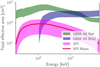 |
Fig. 1 Comparison of the total effective area of GBM and SPI over the SPI energy range. The spread of the lines indicates the full distribution of effective areas depending on the position of the source in the FoV. For SPI, this is restricted to all possible positions in the cFOV and based on the currently valid response version. |
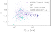 |
Fig. 2 Pair plot of best-fit α and Epeak values for the cut-off power law fit of the GRBs that are well constrained in our sample and those from the time-resolved Fеrтi/GBМ catalogue (with the BEST selection criterion fulfilled). For visual purpose we only include error bars for one typical time bin in the GBM and in the SPI analysis. The uncertainties on the parameters for the SPI data points are given in Table G.1 and those for the Fеrтi/GBМ data points can be found in the time-resolved GBM catalogue in Yu et al. (2016). |
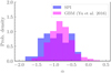 |
Fig. 3 Distribution of best-fit α values for the cut-off power law fit of the GRBs that are well constrained in our sample and those from the time-resolved Fеrтi/GBМ catalogue (with the BEST selection criterion fulfilled). |
4.1.2 The brightest INTEGRAL/SPI GRBs
For the eight brightest GRBs, we checked the temporal evolution of Epeak and α as a function of time (see Figs. C.1 and C.2). General trends are hard to determine, due to the unconstrained peak energy in many time bins and the overall very complex light curve shape of these GRBs. However, the typical drop in peak energy with time can be confirmed for some of the bright single peaks in, for instance, GRBO41219A, GRB061122 and GRB 181201A. For the temporal evolution of α, we can only conclude that it can vary drastically between different pulses in the light curve (e.g. GRB080723B).
4.2 Synchrotron model
4.2.1 The whole sample
Next, we fit the bright GRB sample with Pynchrotron, as described in Sect. 3.2.2 (for one example see Fig. 4). All fits were determined as good fits according to our defined threshold. We also report the values for the electron power law slope p and  for these fits in Table H.1. Here, X determines the synchrotron cooling regime with X < 0 being fast cooling and X > 0 slow cooling. We can see that for most fits, the parameters are not well constrained, which is mostly due to the missing information at high energies. However, for some bright GRBs, we were able to determine the synchrotron cooling regime, and we can clearly see both: time bins with slow-cooling and time bins with fast-cooling.
Identifying the cooling regime of an emission period is important to understand the underlying physics. The emission periods with slow-cooling electron spectra challenge relativistic shock models, as these models depend on a maximum amount of energy conversion into photons via synchrotron emission from the accelerated electrons (Burgess et al. 2020) to overcome their inefficiency of converting internal energy into accelerated electrons (Sari et al. 1996). Our result is in agreement with the findings of Burgess et al. (2020) based on Fermi/GBM data. This is important as it confirms the detection of slow cooling emission periods with another instrument.
4.2.2 The brightest INTEGRAL/SPI GRBs
For the eight brightest GRBs, we show X as a function of time (see Fig. 5). Again, due to the large uncertainties we cannot determine clear trends, but see individual time bins with clear fast and slow cooling. The posteriors for X for all time bins of the brightest SPI GRBs are given in Fig. D.1.
4.2.3 Combining INTEGRAL/SPI with Fermi/GBM data
Combining the data of INTEGRAL/SPI with Fermi/GBM is ideal, as it would include the excellent energy resolution of SPI and the higher effective area (especially at high energies) of GBM (see Fig. 1). Unfortunately, only one very bright GRB in SPI was also seen by GBM, namely, GRB 120711A. It was a very bright burst with Epeak > 1 MeV, at a Redshift z=1.405 (Tanvir et al. 2012), detected by IBAS, GBM, and Konus-Wind (Gotz et al. 2012; Gruber & Pelassa 2012; Golenetskii et al. 2012). Fermi/LAT detected photons > 100 MeV (and up to 2 GeV) in the period between 800 and 7000 seconds after the GRB (Tam et al. 2012). The afterglow was detected in the soft X-rays by XMM-Newton, Chandra, and Swift (Giuliani & Mereghetti, S. 2014; Beardmore & Evans 2012), and in the optical from Watcher, Skynet, GROND, and REM (Lacluyze et al. 2012; Elliott et al. 2012; Fugazza et al. 2012).
In Fig. 6, we show X as a function of time, when we combine SPI and GBM for the spectral fits. For this we included a time offset of −0.37 s between GBM and SPI due to light travel time difference between the satellite positions. For some time bins X can be constrained better, when GBM is included in the fit, that is, the error bar of X is reduced. We also showed this for GRB 120711A in Biltzinger et al. (2022) for the time-integrated spectrum of the brightest peak. Details about the improvements of the model parameters can be found in that paper.
4.3 New INTEGRAL/SPI GRB 190411A
Following the approach described in Sect. 2, we identified two GRBs in the SPI data that are not listed in the IBAS. Both these GRBs were located at the edge of the mask of SPI. One of these two GRBs (GRB 080413) was previously reported in Minaev et al. (2014), but the other (GRB 190411A) was not previously reported for INTEGRAL/SPI.
GRB 190411A2 is a long burst (see Fig. 7) detected also by Fermi/GBM. The GRB localization is RA (2000) = 285°96, Dec(2000) = −36°27), with an error radius of 4.8 degree (statistical only) (von Kienlin et al. 2020). This uncertainty is too large to use for SPI analysis because the response can change drastically in the uncertainty region due to the mask. Therefore, we localised the GRB with the SPI data and PySPI, as in Biltzinger et al. (2022). For this localisation fit, we used a Band function as spectral model and the result is given in Fig. 8. The multi-modality in the localisation could be due to the mask, or could be an artefact from the interpolation of the original 0.5 degree grid of the response. Therefore, we localised GRB 190411A to  and
and  (including a 0.5 degree systematic uncertainty).
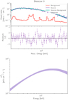 |
Fig. 4 Observed data in the non-PSD energy range of detector 0, over-plotted with the best fit realisation of the synchrotron model for the brightest time bin in our sample (GRB181201A) (top row) and resulting posterior distribution of the vFv spectrum of the GRB (bottom row). |
4.4 GRB signals outside of the coded FoV
To make sure we did not miss any GRB in the SPI data, we performed a search for significant data excess in the SPI data during all detected GRBs since the launch of INTEGRAL. We took the trigger times from the list of all known GRBs3 and calculated the significance of the SPI light curve for the corresponding science window in intervals of 5, 20, and 50 s, centred on the trigger times. If any of the intervals gave a significance greater than five, we checked the light curves manually to filter out observations with non-stable background rates or other obvious problems. For the 39 GRBs (see Table I.1) that are not listed in the IBAS catalogue, a clear signal is visible in the SPI data, with some being quite strong (see e.g. Fig. 9). One especially interesting aspect is that the famous GRB 190114C, detected by MAGIC in the TeV energy range (MAGIC Collaboration 2019), is also visible in the SPI data (see Fig. 10). For all these GRBs there are either previous localisations from other instruments placing the GRB outside of the SPI’s cFOV or our localisation fits fail. We conclude that none of these GRBs is in the cFOV of SPI. Thus, no spectral analysis is possible at the moment. A simulation of the response for positions outside of the cFoV would allow us to analyse these interesting sources in the future. Also, it is important to keep the times of these transient sources in mind when analysing non-transient sources with SPI, as their contribution contaminates the observed data.
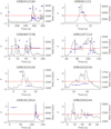 |
Fig. 5 Time evolution of X for the eight brightest GRBs in our sample. Values below (above) the red dashed lines indicates fast (slow) cooling. The light curve are plotted in light grey. |
5 Discussion and conclusion
In this work, we present the first time-resolved INTEGRAL/SPI GRB catalogue. After binning the light curves with the Bayesian block algorithm, we fit all the time intervals fulfilling our data selection criterion with two empirical spectral models: a Band function and cut-off power law. We also fit the very significant time bins (>10σ<) with a physical synchrotron model. We show that the parameter distributions for the cut-off power law fits in our SPI sample are similar to the ones from the time-resolved GBM catalogue in Yu et al. (2016). However, we also note that due to the smaller effective area, which also decreases quickly for photon energies above a few hundred keV, we were not able to constrain the high energy power law slope, unless the GRB was extremely bright or the break energy very low.
We find that the physical synchrotron model is able to fit the data of all time bins well, but often the parameters are not very well constrained. Nevertheless, we identified time bins that are clearly evident either in the slow-cooling or the fast-cooling regime. This is in line with the findings of Burgess et al. (2020), based on the Fermi/GBM data of single-pulsed GRBs. The existence of alternating emission periods in the slow cooling regime could be an indicator of the reheating of electrons, for instance, due to second-order Fermi acceleration (Beniamini et al. 2018; Xu et al. 2018) or magnetic re-connection (Comisso & Sironi 2019). A natural next step in the modelling of synchrotron emission will be to drop the assumption of isotropic pitch angle distributions and to instead use the energy dependent pitch angle distributions found in recent particle in cell (PIC) simulations (Comisso & Sironi 2021).
Finally, we identified one GRB (GRB 190411A) in the SPI data, which was not reported previously with SPI detections. We were able to localise it and our localisation agrees with the one determined by Fermi/GBM.
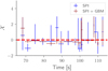 |
Fig. 6 Time evolution of X for GRB120711A for SPI only and SPI+GBM fits. Values below (above) the red dashed lines indicates fast (slow) cooling. |
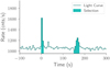 |
Fig. 7 Light curve of GRB 190411 with the data of all SPI detectors summed. The filled area marks the time selection used for the localisation. |
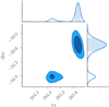 |
Fig. 8 Localisation of GRB 190411A with SPI data. Dark blue (light blue) indicate the 1 (2) sigma confidence regions. This shows the excellent localisation capabilities with PySPI. |
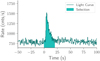 |
Fig. 9 Light curve of the out-oſ-cFoV GRB041212 with the data of all SPI detectors summed as an example of the amount of high-energy photons which are not vetoed by the ACS. The filled area marks the active time of the GRB. |
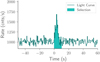 |
Fig. 10 Light curve of GRB 1901l4C with the data of all SPI detectors summed. The filled area marks the active time of the GRB. Due to the detection of this GRB by MAGIC in the TeV energy range (MAGIC Collaboration 2019), this would be a very interesting source to analyse with the SPI data, if an out-oſ-cFoV response will be constructed in the future. |
Acknowledgements
BB acknowledges support from the German Aerospace Center (Deutsches Zentrum für Luft- und Raumfahrt, DLR) under F KZ 50 OR 1913. The INTEGRAL/SPI project has been completed under the responsibility and leadership of CNES; we are grateful to ASI, CEA, CNES, DLR, ESA, INTA, NASA and OSTC for support of this ESA space science mission. We thank the referee for carefully reading the manuscript and giving detailed comments which helped improving the quality of this paper. This work made use of the following software packages: pynchrotron (Burgess et al. 2020), 3ML (Vianello et al. 2015), Astromodels (Vianello et al. 2021), Matplotlib (Caswell et al. 2021), ChainConsumer (Hinton 2016; Hinton et al. 2020), Numpy (Harris et al. 2020), MultiNest (Feroz et al. 2009, 2019; Feroz & Hobson 2008).
Appendix A Detector Selection
For the spectral analysis, we decided to use at most the five detectors with the most significant signal, to assure that the used detectors see the GRB nicely and are not mostly occluded by the tungsten mask elements. This approach was chosen because for some bright GRBs, we were not able to fit the data of the strongly occluded detectors well, while the fits were able to fit the data of the weakly occluded detectors nicely (see Fig. A.1)
This led us to suspect that the response for photons flying through the tungsten mask elements could be significantly worse that for the photons not passing a tungsten mask element. This could be caused by the simplifications made in the original response simulations in Sturner et al. (2003), where the mask effects were simulated with a ray tracing approach to reduce the computational costs of the response simulation significantly or by a slight misalignment of the mask in the simulations with respect to reality. As the detectors with low significance do not contribute much to the spectral analysis, we decided to not include them to avoid this possible source of systematic uncertainties. Additionally, we manually removed detector 12 from the fit for GRB071003, as well as detectors 13 and 3 from the fit for GRB110903, as the fit was not able to explain the data for these detectors.
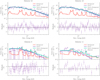 |
Fig. A.1 Observed spectra and best fit model realisations for one time bin of GRB041219 and four different detectors, when fitting a Band function to the data. While the data of the detector with relatively large signal (10 and 18; top row) can be nicely reproduced by the fit, the ones with relatively small signal (4 and 11; bottom row) show systematic over or under fitting in the residuals. |
Appendix B Comparison to the results of Bošnjak et al. (2014)
Bošnjak et al. (2014) performed combined SPI and IBIS spectral fits of time-integrated spectra of all GRBs listed in IBAS up to February 2012. Their results differ sometimes significantly from ours (shown in Table G.1). While some degree of the discrepancy can be assigned to our time-resolved analysis compared to the time integrated analysis in Bošnjak et al. (2014), we examine this discrepancy here in more detail. The data and responses for the analysis in Bošnjak et al. (2014) are publicly available4. With this information, we were able to reconstruct the same data selection criteria (active time, background time, and detectors) with PySPI making a fair comparison between the two analysis possible.
For this, we first fitted the provided SPI and ISGRI data (individually and combined) with the provided response files in 3ML and the models specified in Bošnjak et al. (2014) for the given GRB (power law, cut-off power law, or Band function). Next, we repeated the SPI fits with PySPI for the same model and data selection criteria. The comparison of the resulting low energy slopes (therefore, in case of a Band function the α parameter) is shown in Fig. B.1 for all GRBs listed in Bošnjak et al. (2014), for which the data was available via the ISDC FTP server. It shows that the PySPI results agree with the results for the SPI-only fits of the data provided by Bošnjak et al. (2014), but not with the combined ISGRI+SPI fits. Generally, the results of SPI and ISGRI do not agree with each other for most GRBs, explaining the difference we get with respect to the Bošnjak et al. (2014) results. No tests were done in Bošnjak et al. (2014) to check whether the two instruments give results that are in agreement.
This discrepancy could be due to an inaccurate response of the ISGRI detector, as the response of ISGRI had to be changed constantly to match the results of other instruments (e.g. Savchenko et al. 2014). Additionally, only one very limited cross-calibration analysis for GRB sources was carried out, with only four GRBs and no comparison of the spectral parameters (Tierney et al. 2010). We showed previously in Biltzinger et al. (2022), that the SPI results for the bright GRB 120711A offer a good match with the GBM results.
In this test, we were able to replicate the results given in Bošnjak et al. (2014) for most GRBs, when we took their data files and carried out the combined ISGRI+SPI fit, except for a few GRBs. For instance, the low energy power law of the famous GRB 041219 is ≈ -2 in our case, but is ≈ -1.5 in Bošnjak et al. (2014). We checked the fits for this case and noticed that the fit to the ISGRI data is very inaccurate. After a further investigation of the ISGRI data file provided for GRB 041219, we realised that the data time given in the data files is for the time of GRB 061122 and not GRB 041219. Thereafter, we checked this for all GRBs and found four GRBs in total (GRBs 040422, 041219, 050525, and 060901) where the same error occurred. We marked theses GRBs with wrong data in red color in Fig. B.1. Other GRBs with significantly different results compared to Bošnjak et al. (2014) have a very small fluence (e.g. GRB040422, GRB040827 or GRB090702). These differences can be explained with the different fitting algorithms used: Modified Levenberg-Marquardt algorithm in Bošnjak et al. (2014) and MultiNest in this work. This can lead to different results, especially for weak signals.
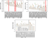 |
Fig. B.1 Comparison of the low energy power law slope in Bošnjak et al. (2014) and our results for the same data selection criterion. The GRBs in these plots are sorted from hard to soft spectra. The GRBs for which the wrong ISGRI data files were provided are marked in red. |
Appendix C Time evolution of cut-off powerlaw parameters
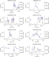 |
Fig. C.1 Time evolution of the peak energy for the cut-off powerlaw fits of the eight brightest SPI GRBs. The light curves are plotted in light grey. |
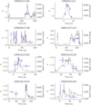 |
Fig. C.2 Time evolution of the power law slope for the cut-off powerlaw fits of the eight brightest SPI GRBs. The light curves are plotted in light grey. |
Appendix D Cooling regime posteriors
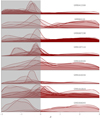 |
Fig. D.1 Posterior distributions for the cooling regime parameter χ for all time bins of the eight brightest SPI GRBs. The grey area marks the fast cooling regime. |
Appendix E QQ-Plot examples
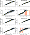 |
Fig. E.1 Example of a good fit (left column) and a bad fit (right column). These plots are for the band function fits of two time slices of GRB190411A. The red intervals mark strong deviations (>95 %) of the true data from the simulated data. |
Appendix F Effective area correction
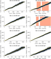 |
Fig. F.1 QQ-plots for band function fit of one time slice of GRB181201. The left (right) column shows the fit with (without) an effective area correction per SPI detector. |
Appendix G Empirical model catalogue
Parameter constrains for empirical model fits. Entries with no parameter values indicate that the fit has failed for this time bin and spectral model and the intensity is given for the energy range of 20-300 keV.
Appendix H Physical synchrotron model catalogue
Parameter constrains for synchrotron model fits. Entries with no parameter values indicate that the fit has failed for this time bin and the intensity is given for the energy range of 20-300 keV.
Appendix I GRBs outside of the FoV
GRBs with significant signal in the SPI detectors but not listed in the IBAS. All of these GRBs were mostly likely outside of the coded FoV.
References
- Band, D., Matteson, J., Ford, L., et al. 1993, ApJ, 413, 281 [Google Scholar]
- Barthelmy, S. D., Barbier, L. M., Cummings, J. R., et al. 2005, Space Sci. Rev., 120, 143 [Google Scholar]
- Beardmore, A., & Evans, P. 2012, GCN Circular 13442 [Google Scholar]
- Beckmann, V., Borkowski, J., Courvoisier, T.-L., et al. 2004, Nucl. Phys. B, Proc. Suppl., 132, 301 [NASA ADS] [CrossRef] [Google Scholar]
- Beniamini, P., Barniol Duran, R., & Giannios, D. 2018, MNRAS, 476, 1785 [NASA ADS] [CrossRef] [Google Scholar]
- Biltzinger, B., Burgess, J. M., & Siegert, T. 2022, J. Open Source Softw., 7, 4017 [NASA ADS] [CrossRef] [Google Scholar]
- Biltzinger, B., Greiner, J., Burgess, J. M., & Siegert, T. 2022, A&A, 663, A102 [NASA ADS] [CrossRef] [EDP Sciences] [Google Scholar]
- Bošnjak, Ž., Götz, D., Bouchet, L., Schanne, S., & Cordier, B. 2014, A&A, 561, A25 [NASA ADS] [CrossRef] [EDP Sciences] [Google Scholar]
- Buchner, J., Georgakakis, A., Nandra, K., et al. 2014, A&A, 564, A125 [NASA ADS] [CrossRef] [EDP Sciences] [Google Scholar]
- Burgess, J. M., Preece, R. D., Connaughton, V., et al. 2014, ApJ, 784, 17 [NASA ADS] [CrossRef] [Google Scholar]
- Burgess, J. M., Bégué, D., Greiner, J., et al. 2020, Nat. Astron., 4, 174 [Google Scholar]
- Caswell, T. A., Droettboom, M., Lee, A., et al. 2021, https://doi.org/10.5281/zenodo.4475376 [Google Scholar]
- Comisso, L., & Sironi, L. 2019, ApJ, 886, 122 [Google Scholar]
- Comisso, L., & Sironi, L. 2021, Phys. Rev. Lett., 127 [Google Scholar]
- Elliott, J., Klose, S., & Greiner, J. 2012, GCN Circular 13438 [Google Scholar]
- Feroz, F., & Hobson, M. P. 2008, MNRAS, 384, 449 [NASA ADS] [CrossRef] [Google Scholar]
- Feroz, F., Hobson, M. P., & Bridges, M. 2009, MNRAS, 398, 1601 [NASA ADS] [CrossRef] [Google Scholar]
- Feroz, F., Hobson, M. P., Cameron, E., & Pettitt, A. N. 2019, The Open Journal of Astrophysics, 2, 10 [NASA ADS] [CrossRef] [Google Scholar]
- Filliatre, P., D’Avanzo, P., Covino, S., et al. 2005, A&A, 438, 793 [NASA ADS] [CrossRef] [EDP Sciences] [Google Scholar]
- Filliatre, P., Covino, S., D’Avanzo, P., et al. 2006, A&A, 448, 971 [NASA ADS] [CrossRef] [EDP Sciences] [Google Scholar]
- Foley, S., McGlynn, S., Hanlon, L., McBreen, S., & McBreen, B. 2008, A&A, 484, 143 [NASA ADS] [CrossRef] [EDP Sciences] [Google Scholar]
- Fugazza, D., Covino, S., & Rossi, A. 2012, GCN Circular 13439 [Google Scholar]
- Gabry, J., Simpson, D., Vehtari, A., Betancourt, M., & Gelman, A. 2017, J. R. Stat. Soc., 182, 389 [Google Scholar]
- Gelman, A. 2003, Int. Stat. Rev., 71, 369 [CrossRef] [Google Scholar]
- Giuliani, A., & Mereghetti, S. 2014, A&A, 563, A6 [NASA ADS] [CrossRef] [EDP Sciences] [Google Scholar]
- Golenetskii, S., R. Aptekar, Frederiks, D., et al. 2012, GCN Circular 13446 [Google Scholar]
- Gotz, D., Mereghetti, S., Bozzo, E., et al. 2012, GCN Circular 13434 [Google Scholar]
- Grebenev, S. A., & Chelovekov, I. V. 2007, Astrophys. Lett., 33, 789 [NASA ADS] [Google Scholar]
- Gruber, D., & Pelassa, V. 2012, GCN Circular 13437 [Google Scholar]
- Harris, C. R., Millman, K. J., van der Walt, S. J., et al. 2020, Nature, 585, 357 [NASA ADS] [CrossRef] [Google Scholar]
- Hinton, S. R. 2016, JOSS, 1, 00045 [NASA ADS] [CrossRef] [Google Scholar]
- Hinton, S., Adams, C., & Badger, C. 2020, https://doi.org/10.5281/zenodo.4280904 [Google Scholar]
- Kumar, P., & Zhang, B. 2015, Phys. Rep., 561, 1 [Google Scholar]
- Lacluyze, A., Haislip, J., Ivarsen, K., et al. 2012, GCN Circular 13430 [Google Scholar]
- Li, T. P., & Ma, Y. Q. 1983, ApJ, 272, 317 [CrossRef] [Google Scholar]
- Lien, A., Sakamoto, T., Barthelmy, S. D., et al. 2016, ApJ, 829, 7 [Google Scholar]
- MAGIC Collaboration (Acciari, V. A., et al.) 2019, Nature, 575, 455 [Google Scholar]
- Malaguti, G., Bazzano, A., Beckmann, V., et al. 2003, A&A, 411, L307 [NASA ADS] [CrossRef] [EDP Sciences] [Google Scholar]
- Martin-Carrillo, A., Hanlon, L., Topinka, M., et al. 2014, A&A, 567, A84 [NASA ADS] [CrossRef] [EDP Sciences] [Google Scholar]
- McBreen, S., Hanlon, L., McGlynn, S., et al. 2006, A&A, 455, 433 [NASA ADS] [CrossRef] [EDP Sciences] [Google Scholar]
- McGlynn, S., Foley, S., McBreen, S., et al. 2008, A&A, 486, 405 [NASA ADS] [CrossRef] [EDP Sciences] [Google Scholar]
- McGlynn, S., Foley, S., McBreen, B., et al. 2009, A&A, 499, 465 [NASA ADS] [CrossRef] [EDP Sciences] [Google Scholar]
- Mereghetti, S., Götz, D., Borkowski, J., Walter, R., & Pedersen, H. 2003, A&A, 411, L291 [NASA ADS] [CrossRef] [EDP Sciences] [Google Scholar]
- Mereghetti, S., Gtz, D., Tiengo, A., et al. 2003, ApJ, 590, L73 [NASA ADS] [CrossRef] [Google Scholar]
- Minaev, P. Y., Pozanenko, A. S., Molkov, S. V., & Grebenev, S. A. 2014, Astron. Lett., 40, 235 [NASA ADS] [CrossRef] [Google Scholar]
- Moran, L., Mereghetti, S., Götz, D., et al. 2005, A&A, 432, 467 [NASA ADS] [CrossRef] [EDP Sciences] [Google Scholar]
- Oganesyan, G., Nava, L., Ghirlanda, G., Melandri, A., & Celotti, A. 2019, A&A, 628, A59 [NASA ADS] [CrossRef] [EDP Sciences] [Google Scholar]
- Ronchi, M., Fumagalli, F., Ravasio, M. E., et al. 2020, A&A, 636, A55 [NASA ADS] [CrossRef] [EDP Sciences] [Google Scholar]
- Roques, J.-P., & Jourdain, E. 2019, ApJ, 870, 92 [NASA ADS] [CrossRef] [Google Scholar]
- Rybicki, G. B., & Lightman, A. P. 1986, Radiative Processes in Astrophysics (Wiley-VCH) [Google Scholar]
- Sari, R., Narayan, R., & Piran, T. 1996, ApJ, 473, 204 [Google Scholar]
- Savchenko, V., Lebrun, F., & Laurent, P. 2014, in Proceedings of Science, 10th INTEGRAL Workshop: A Synergistic View of the High-Energy Sky [Google Scholar]
- Scargle, J. D., Norris, J. P., Jackson, B., & Chiang, J. 2013, ApJ, 764, 167 [Google Scholar]
- Sturner, S. J., Shrader, C. R., Weidenspointner, G., et al. 2003, A&A, 411, L81 [NASA ADS] [CrossRef] [EDP Sciences] [Google Scholar]
- Tam, P., Li, K., & Kong, A. 2012, GCN Circular 13444 [Google Scholar]
- Tanvir, N. R., Wiersema, K., Levan, A. J., et al. 2012, GCN Circular 13441 [Google Scholar]
- Tierney, D., McBreen, S., Fermi Gbm Team, et al. 2010, in Eighth Integral Workshop. The Restless Gamma-ray Universe (INTEGRAL 2010), 103 [Google Scholar]
- Vedrenne, G., Roques, J. P., Schönfelder, V., et al. 2003, A&A, 411, L63 [NASA ADS] [CrossRef] [EDP Sciences] [Google Scholar]
- Vianello, G., Lauer, R. J., Younk, P., et al. 2015, arXiv e-prints, [arXiv:1507.08343] [Google Scholar]
- Vianello, G., Burgess, J., Fleischhack, H., Di Lalla, N., & Omodei, N. 2021, https://doi.org/10.5281/zenodo.5646925 [Google Scholar]
- von Kienlin, A., et al. 2020, ApJ, 893, 46 [NASA ADS] [CrossRef] [Google Scholar]
- von Kienlin, A., Beckmann, V., Covino, S., et al. 2003a, A&A, 411, L321 [NASA ADS] [CrossRef] [EDP Sciences] [Google Scholar]
- von Kienlin, A., Beckmann, V., Rau, A., et al. 2003b, A&A, 411, L299 [NASA ADS] [CrossRef] [EDP Sciences] [Google Scholar]
- Wilk, M. B., & Gnanadesikan, R. 1968, Biometrika, 55, 1 [Google Scholar]
- Winkler, C., Courvoisier, T. J. L., Di Cocco, G., et al. 2003, A&A, 411, L1 [NASA ADS] [CrossRef] [EDP Sciences] [Google Scholar]
- Xu, S., Yang, Y.-P., & Zhang, B. 2018, ApJ, 853, 43 [NASA ADS] [CrossRef] [Google Scholar]
- Yu, H.-F., Preece, R. D., Greiner, J., et al. 2016, A&A, 588, A135 [NASA ADS] [CrossRef] [EDP Sciences] [Google Scholar]
All Tables
Parameter constrains for empirical model fits. Entries with no parameter values indicate that the fit has failed for this time bin and spectral model and the intensity is given for the energy range of 20-300 keV.
Parameter constrains for synchrotron model fits. Entries with no parameter values indicate that the fit has failed for this time bin and the intensity is given for the energy range of 20-300 keV.
GRBs with significant signal in the SPI detectors but not listed in the IBAS. All of these GRBs were mostly likely outside of the coded FoV.
All Figures
|
Fig. 1 Comparison of the total effective area of GBM and SPI over the SPI energy range. The spread of the lines indicates the full distribution of effective areas depending on the position of the source in the FoV. For SPI, this is restricted to all possible positions in the cFOV and based on the currently valid response version. |
| In the text | |
|
Fig. 2 Pair plot of best-fit α and Epeak values for the cut-off power law fit of the GRBs that are well constrained in our sample and those from the time-resolved Fеrтi/GBМ catalogue (with the BEST selection criterion fulfilled). For visual purpose we only include error bars for one typical time bin in the GBM and in the SPI analysis. The uncertainties on the parameters for the SPI data points are given in Table G.1 and those for the Fеrтi/GBМ data points can be found in the time-resolved GBM catalogue in Yu et al. (2016). |
| In the text | |
|
Fig. 3 Distribution of best-fit α values for the cut-off power law fit of the GRBs that are well constrained in our sample and those from the time-resolved Fеrтi/GBМ catalogue (with the BEST selection criterion fulfilled). |
| In the text | |
|
Fig. 4 Observed data in the non-PSD energy range of detector 0, over-plotted with the best fit realisation of the synchrotron model for the brightest time bin in our sample (GRB181201A) (top row) and resulting posterior distribution of the vFv spectrum of the GRB (bottom row). |
| In the text | |
|
Fig. 5 Time evolution of X for the eight brightest GRBs in our sample. Values below (above) the red dashed lines indicates fast (slow) cooling. The light curve are plotted in light grey. |
| In the text | |
|
Fig. 6 Time evolution of X for GRB120711A for SPI only and SPI+GBM fits. Values below (above) the red dashed lines indicates fast (slow) cooling. |
| In the text | |
|
Fig. 7 Light curve of GRB 190411 with the data of all SPI detectors summed. The filled area marks the time selection used for the localisation. |
| In the text | |
|
Fig. 8 Localisation of GRB 190411A with SPI data. Dark blue (light blue) indicate the 1 (2) sigma confidence regions. This shows the excellent localisation capabilities with PySPI. |
| In the text | |
|
Fig. 9 Light curve of the out-oſ-cFoV GRB041212 with the data of all SPI detectors summed as an example of the amount of high-energy photons which are not vetoed by the ACS. The filled area marks the active time of the GRB. |
| In the text | |
|
Fig. 10 Light curve of GRB 1901l4C with the data of all SPI detectors summed. The filled area marks the active time of the GRB. Due to the detection of this GRB by MAGIC in the TeV energy range (MAGIC Collaboration 2019), this would be a very interesting source to analyse with the SPI data, if an out-oſ-cFoV response will be constructed in the future. |
| In the text | |
|
Fig. A.1 Observed spectra and best fit model realisations for one time bin of GRB041219 and four different detectors, when fitting a Band function to the data. While the data of the detector with relatively large signal (10 and 18; top row) can be nicely reproduced by the fit, the ones with relatively small signal (4 and 11; bottom row) show systematic over or under fitting in the residuals. |
| In the text | |
|
Fig. B.1 Comparison of the low energy power law slope in Bošnjak et al. (2014) and our results for the same data selection criterion. The GRBs in these plots are sorted from hard to soft spectra. The GRBs for which the wrong ISGRI data files were provided are marked in red. |
| In the text | |
|
Fig. C.1 Time evolution of the peak energy for the cut-off powerlaw fits of the eight brightest SPI GRBs. The light curves are plotted in light grey. |
| In the text | |
|
Fig. C.2 Time evolution of the power law slope for the cut-off powerlaw fits of the eight brightest SPI GRBs. The light curves are plotted in light grey. |
| In the text | |
|
Fig. D.1 Posterior distributions for the cooling regime parameter χ for all time bins of the eight brightest SPI GRBs. The grey area marks the fast cooling regime. |
| In the text | |
|
Fig. E.1 Example of a good fit (left column) and a bad fit (right column). These plots are for the band function fits of two time slices of GRB190411A. The red intervals mark strong deviations (>95 %) of the true data from the simulated data. |
| In the text | |
|
Fig. F.1 QQ-plots for band function fit of one time slice of GRB181201. The left (right) column shows the fit with (without) an effective area correction per SPI detector. |
| In the text | |
Current usage metrics show cumulative count of Article Views (full-text article views including HTML views, PDF and ePub downloads, according to the available data) and Abstracts Views on Vision4Press platform.
Data correspond to usage on the plateform after 2015. The current usage metrics is available 48-96 hours after online publication and is updated daily on week days.
Initial download of the metrics may take a while.