© The Authors 2023

1. Introduction

The broad emission lines with velocity widths of ∼1000–20 000 km s⁻¹ seen as prominent features in the UV and optical spectra of active galactic nuclei (AGNs) originate from broad-line regions (BLRs) photoionized by the continuum radiation from the central accretion disks around supermassive black holes (SMBHs). The physics of BLRs (e.g., the geometry, kinematics, mass distributions, and photoionization properties), which determines the profiles of broad emission lines, is not only related to the origin and evolution of the materials in the central regions of AGNs, but is also closely related to the measurement of BH masses in reverberation mapping (RM, e.g., Blandford & McKee 1982; Peterson 1993). This makes BLRs one of the core topics in AGN researches.

Reverberation mapping is a technique used to probe the geometry and kinematics of BLRs and to measure the masses of SMBHs in AGNs. It has been successfully applied to more than 100 objects in recent decades (e.g., Peterson et al. 1998; Kaspi et al. 2000; Bentz et al. 2009; Denney et al. 2009; Barth et al. 2011; Rafter et al. 2011; Du et al. 2014, 2018a; Fausnaugh et al. 2017; Grier et al. 2017a; De Rosa et al. 2018; Rakshit et al. 2019; Hu et al. 2021; Yu et al. 2021; Bao et al. 2022). RM measures the delayed response of broad emission lines with respect to the varying continuum emission. Due to the limits of spectral resolution and flux calibration precision, most of the early RM campaigns focused on the average time lags (τ_Hβ) of the Hβ emission line (e.g., Peterson et al. 1998; Kaspi et al. 2000). In combination with the velocity widths (V_Hβ) of Hβ lines, the masses of SMBHs can be formulated with $M_{•}=f_{\text{BLR}}{V}_{\text{H}\beta }^2{R}_{\text{H}\beta }/G$, where R_Hβ = cτ_Hβ is the emissivity-weighted radius of BLR, c is the speed of light, G is the gravitational constant, and f_BLR is a parameter called the “virial factor”, which is controlled by the BLR geometry and kinematics. Therefore, the accuracy of BH mass measurement is directly related to our understanding of BLR physics. Furthermore, with the improvement of flux calibration and spectral resolution in recent years, velocity-resolved RM, rather than only measuring an average time lag, is being performed on an increasing number of objects. The aim of velocity-resolved RM is to measure the time lag as a function of velocity (e.g., Bentz et al. 2008, 2010a; Denney et al. 2010; Du et al. 2016b, 2018b; Pei et al. 2017; De Rosa et al. 2018; Hu et al. 2020a,b; Brotherton et al. 2020; Lu et al. 2021; Vivian et al. 2022; Bao et al. 2022) or, more importantly, to reconstruct the “velocity-delay maps” (also known as transfer functions) of BLRs using model-independent methods such as the maximum entropy method (e.g., Bentz et al. 2010b; Grier et al. 2013; Skielboe et al. 2015; Xiao et al. 2018a,b; Brotherton et al. 2020; Horne et al. 2021) and to constrain the BLR parameters by Bayesian modeling through a Markov Chain Monte Carlo approach (MCMC, e.g., Pancoast et al. 2012, 2014; Grier et al. 2017b; Williams et al. 2018; Li et al. 2018; Villafaña et al. 2022). The general geometry and kinematics of the BLRs (e.g., disk-like, inflow, or outflow) in dozens of AGNs have been successfully revealed (see the aforementioned references).

Systematic studies on inhomogeneity and substructures in BLRs are relatively scarce, but three pieces of evidence may have indicated their existence: (1) Many AGNs show complex emission-line profiles, even with multiple wiggles or small peaks, rather than symmetric profiles or simply asymmetric profiles with a little stronger red or blue wings in their emission lines (e.g., the line profiles of Mrk 6, Mrk 715, or NGC 2617 in the appendix Du et al. 2018b). This indicates that the BLR gas distributions in those objects should be more complex than previously thought. (2) There is a well-known phenomenon that the line profiles in the mean and rms spectra of RM are commonly different for the same object (e.g., Peterson et al. 1998; Bentz et al. 2009; Denney et al. 2009; Barth et al. 2013; Fausnaugh et al. 2017; Grier et al. 2012; Du et al. 2018b; De Rosa et al. 2018; Brotherton et al. 2020). The profiles of the emission lines in rms spectra represent the geometry and kinematics of the gas that responds to the continuum variations and is only a portion of the total BLR gas. The differences between the mean and rms spectra suggest gas inhomogeneity in BLRs. (3) More importantly, the velocity-delay maps of some objects (e.g., NGC 5548) have shown complex features (e.g., incomplete ellipse, bright strips) in comparison with the simple disk, inflow, or outflow models. These are probably evidence of BLR inhomogeneity and substructures (e.g., Xiao et al. 2018b; Horne et al. 2021).

The radii of BLRs measured by RM mostly span from 10³R_g to 10⁵R_g for different objects, where R_g = 1.5 × 10¹³M₈ cm is the gravitational radius and M₈ = M_•/10⁸ M_⊙ is the SMBH mass in units of 10⁸ solar masses (Du et al. 2016a). Such a range of radius is consistent with the self-gravitating region of the accretion disk (e.g., Paczynski 1978; Shlosman & Begelman 1987; Bertin & Lodato 1999; Goodman 2003; Sirko & Goodman 2003). In addition, a number of objects (e.g., Arp 151, 3C 120, NGC 5548) show clear RM signatures of Keplerian disks (Bentz et al. 2010b; Grier et al. 2013; Xiao et al. 2018b; Horne et al. 2021). The heuristic idea that the origin of BLRs is related to the self-gravitating regions of accretion disks was initially discussed by Shore & White (1982), and was further theoretically studied in the subsequent works (e.g., Collin-Souffrin 1987; Collin-Souffrin & Dumont 1990; Dumont & Collin-Souffrin 1990a,b). Although the detailed physics in the self-gravitating region is still far from fully understood, the existence of spiral arms may be a natural consequence resulting from the gravitational instabilities in this region (e.g., Lodato 2007).

On the other hand, the mass ratio of the standard accretion disk (Shakura & Sunyaev 1973) to SMBH can be expressed as $0.04{\alpha }_{0.1}^{-4/5}{M}_8^{6/5}{\dot{\mathcal{M}}}^{7/10}{r}_4^{5/4}$ (or $0.7{\alpha }_{0.1}^{-4/5}{M}_8^{6/5}{\dot{\mathcal{M}}}^{7/10}{r}_5^{5/4}$ depending on the typical radius) if the disk extends to the scale size of the BLR, where $\dot{\mathcal{M}}={\dot{M}}_{\bullet }{c}^2/L_{\mathrm{Edd}}$ is the dimensionless accretion rate, Ṁ_∙ is the mass-accretion rate, L_Edd = 1.5 × 10⁴⁶M₈ erg s⁻¹ is the Eddington luminosity of gas of solar composition, α_0.1 = α/0.1 is the viscosity parameter, and r₄ = R_out/10⁴R_g (or r₅ = R_out/10⁵R_g) is the outer radius. This ratio is generally similar to the disk-to-star mass ratios in protoplanetary systems, which commonly possess spiral-arm structures (e.g., Andrews et al. 2013; Dong et al. 2018). This also leads to the possibility that BLRs can host spiral arms.

Therefore, it is important to investigate the spiral arms in BLRs and their potential characteristics in observations. Horne et al. (2004) calculated the velocity-delay map of a photoionized disk with two spiral arms mathematically without introducing any precise physics (through “twisting” the elliptical orbits). Gilbert et al. (1999), Storchi-Bergmann et al. (2003), Schimoia et al. (2012), and Storchi-Bergmann et al. (2017) assumed an analytical form for the spiral arms and explained the double-peaked profiles of the broad emission lines in AGNs, but similarly did not include any dynamical physics. As the first paper of this series, Wang et al. (2022) used notions of density wave theory of spiral galaxies (e.g., Lin & Shu 1964, 1966; Lin et al. 1969), which applies to self-gravitating disks (Goldreich & Tremaine 1979), to investigate BLRs for the first time (hereafter Paper I). Paper I explores the possibility of density waves in BLRs through discussing their physical conditions, and focuses on the simplest cases of tight-winding arms with short wavelengths and small pitch angles (adopting the formalism of the tight-winding approximation). However, the loosely wound spiral arms have more significant features in line profiles or RM signals than the tightly wound cases (see more details in Paper I or in the following sections of the present paper). It is therefore crucial to investigate the loosely wound spiral arms in BLRs and their characteristics in observations.

As the second paper of this series, here we calculate the surface density distributions of loosely wound spiral arms in a numerical manner without the tight-winding approximation, and their corresponding emission-line profiles, velocity-delay maps, and velocity-resolved lags. Comparing with Paper I, we adopt more general radial distributions of the BLR surface density and sound speed, which are assumed as power laws with free indexes. This is a natural extension of Paper I. The paper is organized as follows. In Sect. 2, we briefly introduce the density wave model and the numerical method. Some fiducial modes (arm patterns) and their observational signals (in emission-line profiles, velocity-delay maps, and velocity-resolved lags) for different azimuthal angles of the line of sight (LOS) are provided in Sects. 3 and 4. We discuss and compare the models with the observations in Sect. 5. A brief summary is given in Sect. 6.

2. Theoretical formulation

We adopt the density wave formalism given by Lin & Lau (1979) and the numerical method presented by Adams et al. (1989) to calculate the spiral arms. The perturbation equations and numerical method in Adams et al. (1989) apply to both tightly and loosely wound arms, and can also be used to derive the one-armed density wave (azimuthal wave number m = 1). Details of the formulae and numerical procedures can be found in these papers and the references therein. For completeness, we briefly describe the key points in this section. The general geometry of the BLR modeled in the present paper is disk-like and the model can therefore be applied to objects that show clear features of Keplerian disks in their RM signals (e.g., Arp 151, 3C 120, NGC 5548 in Bentz et al. 2010b; Grier et al. 2013; Xiao et al. 2018b; Horne et al. 2021).

2.1. Perturbation equations

Here, we adopt the linear normal-mode formalism in Adams et al. (1989) (we also refer to the more recent work of Chen et al. 2021). We use the cylindrical coordinates (R, φ, z). In a thin disk, the continuity equation and the motion equations in radial and azimuthal directions read

$$\begin{array}{c}\hfill \frac{\partial \sigma }{\partial t}+\frac{1}{R}\frac{\partial }{\partial R}(R\sigma u)+\frac{1}{R}\frac{\partial }{\partial \phi }(\sigma \upsilon )=0,\end{array}$$(1)

$$\begin{array}{c}\hfill \frac{\partial u}{\partial t}+u\frac{\partial u}{\partial R}+\frac{\upsilon }{R}\frac{\partial u}{\partial \phi }-\frac{{\upsilon }^2}{R}=-\frac{\partial }{\partial R}({\mathcal{V}}_0+\psi +h),\end{array}$$(2)

and

$$\begin{array}{c}\hfill \frac{\partial \upsilon }{\partial t}+u\frac{\partial \upsilon }{\partial R}+\frac{\upsilon }{R}\frac{\partial \upsilon }{\partial \phi }+\frac{u\upsilon }{R}=-\frac{1}{R}\frac{\partial }{\partial \phi }(\psi +h),\end{array}$$(3)

respectively, where u(R, φ, t) and υ(R, φ, t) are the radial and azimuthal components of velocity, σ(R, φ, t) is the surface density, 𝒱₀ is the gravitational potential of SMBH, ψ is the gravitational potential of a disk, h is the enthalpy defined by dh = a²dσ/σ (governed by the thermodynamic property of gas), and a is the sound speed. It should be noted that the viscosity is neglected here.

The m-fold linear perturbations of the equilibrium state are considered. The variables (u, υ, σ, ψ, h) can be expressed as F(R, φ, t) = F₀(R)+F₁(R)e^{i(ωt − mφ)}, where F is u, υ, σ, ψ, or h. The subscript 0 represents the variables in the equilibrium state, and 1 represents the perturbation components. ω = mΩ_p − iγ is the complex eigenfrequency; its real part represents the pattern speed Ω_p of the rotating arms, and the imaginary part gives the exponential growth rate γ of the density waves. The linearized equations can then be formulated as

$$\begin{array}{c}\hfill \frac{1}{R}\frac{\mathrm{d}}{\mathrm{d}R}(R{\sigma }_0{u}_1)-\frac{\mathit{im}}{R}{\sigma }_0{\upsilon }_1+i(\omega -m\mathrm{\Omega }){\sigma }_1=0,\end{array}$$(4)

$$\begin{array}{c}\hfill i(\omega -m\mathrm{\Omega })u_1-2\mathrm{\Omega }{\upsilon }_1=-\frac{\mathrm{d}({\psi }_1+h_1)}{\mathrm{d}R},\end{array}$$(5)

and

$$\begin{array}{c}\hfill \frac{{\kappa }^2}{2\mathrm{\Omega }}{u}_1+i(\omega -m\mathrm{\Omega }){\upsilon }_1=im\frac{{\psi }_1+h_1}{R},\end{array}$$(6)

where Ω(r) is the rotation curve and κ is the epicyclic frequency.

The perturbation ψ₁ of the gravitational potential can be given by the integral of the surface density

$$\begin{array}{c}\hfill {\psi }_1(R)=-G{\displaystyle {\int }_{R_{\mathrm{in}}}^{R_{\mathrm{out}}}\mathrm{d}\zeta {\int }_0^{2\pi }\frac{\zeta {\sigma }_1(\zeta )cos(m\phi )\mathrm{d}\phi }{\sqrt{R^2+{\zeta }^2-2\zeta Rcos\phi }},}\end{array}$$(7)

where R_in and R_out are the inner and outer radius of the disk.

Combining the above equations, we can obtain the integro-differential equation of ψ₁ and σ₁:

$$\begin{array}{c}\hfill [\frac{{\mathrm{d}}^2}{\mathrm{d}{R}^2}+\mathcal{A}\frac{\mathrm{d}}{\mathrm{d}R}+\mathcal{B}](h_1+{\psi }_1)=-\mathcal{C}{h}_1,\end{array}$$(8)

where

$$\begin{array}{c}\hfill \mathcal{A}=-\frac{\mathrm{d}}{\mathrm{d}R}ln\left[\frac{{\kappa }^2(1-{\nu }^2)}{{\sigma }_{0}R}\right],\end{array}$$(9)

$$\begin{array}{c}\hfill \mathcal{B}=-\frac{m^2}{R^2}-\frac{4m\mathrm{\Omega }(R{\nu }^{\prime })}{\kappa R^2(1-{\nu }^2)}+\frac{2m\mathrm{\Omega }}{R^2\kappa \nu }\frac{\mathrm{d}ln({\kappa }^2/{\sigma }_0\mathrm{\Omega })}{\mathrm{d}lnR},\end{array}$$(10)

$$\begin{array}{c}\hfill \mathcal{C}=-\frac{{\kappa }^2(1-{\nu }^2)}{a_0^2},\end{array}$$(11)

$$\begin{array}{c}\hfill h_1=a_0^2\frac{{\sigma }_1}{{\sigma }_0},\end{array}$$(12)

and ν = (ω − mΩ)/κ is the dimensionless frequency. Equation (8) is the governing integro-differential equation of the density wave. Solving this equation numerically, if given the boundary conditions, can provide the perturbation of the surface density σ₁. Considering that the spiral arms in galaxies (e.g., Sugai & Iye 1995; Aryal & Saurer 2004, 2005) or protoplanetary disks (e.g., Pérez et al. 2016; Huang et al. 2018) are mostly trailing (trailing waves can transport angular momentum outward; see e.g., Lin & Lau 1979), we only investigate the cases of trailing waves in BLRs in the present paper.

2.2. Rotation curve

For the SMBH and BLR disk system, the rotation curve has three components (see Adams et al. 1989):

$$\begin{array}{c}\hfill {\mathrm{\Omega }}^2(r)=\frac{G{M}_{\bullet }}{R^3}+\frac{1}{R}\frac{\mathrm{d}{\psi }_0}{\mathrm{d}R}+\frac{1}{R}\frac{\mathrm{d}{h}_0}{\mathrm{d}R},\end{array}$$(13)

which come from the central SMBH, the unperturbed disk, and the pressure, respectively. The disk component can be expressed as

$$\begin{array}{c}\hfill {\psi }_0(R)=-G{\displaystyle {\int }_{R_{\mathrm{in}}}^{R_{\mathrm{out}}}\mathrm{d}\zeta {\int }_0^{2\pi }\frac{\zeta {\sigma }_0(\zeta )\mathrm{d}\phi }{\sqrt{R^2+{\zeta }^2-2\zeta Rcos\phi }}.}\end{array}$$(14)

Given the rotation curve, the epicyclic frequency can be written as

$$\begin{array}{c}\hfill {\kappa }^2=\frac{1}{R^3}\frac{\mathrm{d}{(R^2\mathrm{\Omega })}^2}{\mathrm{d}R}.\end{array}$$(15)

As is well known, the elliptic integral in the calculation of disk potential has singularity (e.g., Adams et al. 1989; Laughlin et al. 1997; Huré 2005). Some methods can handle this singularity in specific cases; for example, the splitting method in Huré et al. (2007). Here, we follow Adams et al. (1989) and use the softened gravity method to calculate the disk potential. A softening term of η²R² is added into the square root of the denominator at the singular points. We adopt η = 0.1 in the calculation of the rotation curve, and checked that the deduced Ω(R) is similar to that obtained by the splitting method in Huré et al. (2007). For Eq. (7), we use a smaller value of η = 0.01 similar to Chen et al. (2021). We also checked that the detailed values of the softening parameter η do not significantly change the spiral arms, emission-line profiles, or velocity-delay maps in the following sections¹. However, it should be noted that the softening parameter η may influence the growth rate of the density wave (e.g., Laughlin et al. 1997), though it may not significantly change the spiral pattern (particularly away from the corotation or Lindblad resonances, where ν = 0 or ±1). We mainly focus on the spiral pattern and the corresponding RM characteristics in the present paper. The influence of η to the growth rate will be discussed in a future paper.

2.3. Boundary conditions

The origin of BLRs is still under debate (e.g., Czerny & Hryniewicz 2011; Wang et al. 2017). Although the emissivity-averaged radii of BLRs (R_BLR) have been measured in more than 100 AGNs by RM campaigns (see, e.g., Bentz et al. 2013; Du et al. 2015; Du & Wang 2019; Grier et al. 2017a), the inner and outer radii of BLRs and their corresponding boundary conditions have large uncertainties so far. However, the radii of dusty tori in some AGNs have been successfully measured, which give us strong constraints on the outer radii of their BLRs. Infrared RM campaigns found a relation between the radius for the innermost dusty torus and the optical luminosity, which is written as $R_{\mathrm{torus}}\approx 0.1L_{43.7}^{0.5}\mathrm{pc}$ (e.g., Minezaki et al. 2019). Here, L_43.7 is the V-band luminosity in units of 10^43.7 erg s⁻¹. We adopt a typical bolometric correction factor of 10 (from bolometric to V-band luminosity). We set the outer radius of the BLR at the inner edge of the dusty torus in our calculation (R_out = R_torus). Considering R_torus/R_BLR ≈ 3 ∼ 7 (Du et al. 2015; Minezaki et al. 2019), we adopt R_out/R_in = 20, 50, 100 in the following calculations in order to ensure that the radial range of our calculation is sufficiently wide, and to check the influence of different R_out/R_in on the spiral arms.

We adopt the same boundary conditions as in Adams et al. (1989) for simplicity, but keep in mind that the detailed BLR boundary conditions are still unknown. At the outer boundary, we assume that the Lagrangian pressure perturbation vanish, which means the confining pressure from the external medium (probably the gas in the torus) is a constant. At the inner boundary, we assume the velocity perturbation u₁ = 0, so that the radial component of the velocity perturbation vanishes at the inner boundary. Inner and outer boundary conditions can be verified by comparing the arm patterns and the corresponding emission profiles, velocity-resolved lags, and velocity-delay maps with RM observations in the future.

2.4. Indirect potential for one-armed density wave

Adams et al. (1989) considered the influence of the one-armed perturbation for the first time, which causes the center of the star to be displaced from the center of mass of the protoplanetary system. We also take this effect into account in our calculation using the same method, incorporating an indirect potential component in Eq. (8) as in Adams et al. (1989). The indirect potential can be expressed as

$$\begin{array}{c}\hfill {\stackrel{\sim }{\psi }}_1=\frac{\pi {\omega }^{2}R}{M_{\bullet }+M_{\mathrm{disk}}}{\displaystyle {\int }_{R_{\mathrm{in}}}^{R_{\mathrm{out}}}{\zeta }^2{\sigma }_1(\zeta )\mathrm{d}\zeta ,}\end{array}$$(16)

where M_disk is the mass of the BLR disk.

2.5. Numerical method

Exact numerical schemes for solving Eq. (8) were presented in Pannatoni & Lau (1979) or Adams et al. (1989) for example. In the present paper, we adopt the matrix scheme in Adams et al. (1989) for searching the eigenvalues of ω and solving the governing integro-differential equation. The details of the matrix scheme can be found in Adams et al. (1989). We only briefly describe the general idea and some key points here. The integral and differential operators in Eq. (8) can be expressed as matrices. By introducing the dimensionless surface-density perturbation S(R) defined by σ₁(R) = σ₀(R)S(R) and dividing the radial axis into N grid in logarithmic space, the integro-differential equation can be reduced to the form

$$\begin{array}{c}\hfill {\mathcal{W}}_{\mathit{ik}}(\omega )S_k=0,\end{array}$$(17)

where i, k = 1, …, N are the indices of the radial grid. The repeated subscript implies summation over its range as the convention in matrix manipulation. The first and last row of the matrix 𝒲_ik(ω) are determined by the inner and outer boundary conditions. Equation (17) is a homogeneous system with N equations and N unknowns, and only has nonzero solutions if the matrix 𝒲_ik(ω) has a vanishing determinant, which can yield the eigenvalue of ω. The matrix 𝒲_ik(ω) is a fifth-order function of ω.

To find all of the eigenvalues simultaneously, Eq. (17) is rewritten into a 5N × 5N matrix equation

$$\begin{array}{c}\hfill {\stackrel{\sim }{\mathcal{W}}}_{\mathit{nl}}^1{S}_l^{\ast }=\omega {\stackrel{\sim }{\mathcal{W}}}_{\mathit{nl}}^2{S}_l^{\ast },\end{array}$$(18)

where n, l = 1, …, 5N are indices, ${\stackrel{\sim }{\mathcal{W}}}_{\mathit{nl}}^1$ and ${\stackrel{\sim }{\mathcal{W}}}_{\mathit{nl}}^2$ are two matrices regrouped from 𝒲_ik(ω) in light of the coefficients of ω with different orders, and $S_l^{*}$ is a rearrangement of S_k (see its detailed form in Adams et al. 1989 and Appendix B). We can obtain the eigenvalues ω and eigenvectors S by solving this generalized eigenvalue problem. Equation (18) has 5N eigenvalues, which corresponds to 5N modes. Most of the modes have zero growth rate (imaginary part; see Sect. 2.1 and Appendix A) and are not physically relevant. We select the lowest-order mode with significant growth rate, which will span the largest radial range and can be self-excited to become significant. For efficiency in calculations, we use N = 500 in the present paper.

3. Patterns of spiral arms

3.1. Fiducial models

Before solving the governing equation, the equilibrium state of the BLR is required. The emissivity distributions of BLRs have been preliminarily reconstructed through BLR modeling in several objects (e.g., Pancoast et al. 2012, 2014; Grier et al. 2017b; Williams et al. 2018; Li et al. 2018); however, the real surface density distributions are still unclear because the reprocessing coefficient distributions are not known. In Paper I, we adopt the polytropic relation as the prescription of the disk. Here, we generalize and assume that the distributions of the surface density and sound speed are power laws, which follow

$$\begin{array}{c}\hfill {\sigma }_0(R)={\widehat{\sigma }}_0{\left(\frac{R}{R_{\mathrm{in}}}\right)}^{-p},\end{array}$$(19)

and

$$\begin{array}{c}\hfill a_0(R)={\widehat{a}}_0{\left(\frac{R}{R_{\mathrm{in}}}\right)}^{-q/2}.\end{array}$$(20)

We use q/2 rather than q as the index of a₀ in order to remain consistent with the approach taken by Adams et al. (1989).

The stability of a disk can be quantified by the parameter Q = κa₀/πGσ₀ (Toomre 1964). The disk is stable if Q ≫ 1, and very unstable if Q is far smaller than unity. Here, we consider a quasi-stable BLR disk with average Q parameter value, which is defined by

$$\begin{array}{c}\hfill \overline{Q}=\frac{{\int }_{R_{\mathrm{in}}}^{R_{\mathrm{out}}}2\pi RQ{\sigma }_0\mathrm{d}R}{{\int }_{R_{\mathrm{in}}}^{R_{\mathrm{out}}}2\pi R{\sigma }_0\mathrm{d}R},\end{array}$$(21)

which is close to unity. We set $\overline{Q}$ as a free parameter in the following sections.

In total, the model used here has seven parameters: the mass of SMBH M_•, the mass ratio between disk and SMBH M_disk/M_•, the dimensionless accretion rate $\dot{\mathcal{M}}$, the power law indices p and q, parameter $\overline{Q}$, and the ratio of outer and inner radii R_out/R_in. Among them, M_• and $\dot{\mathcal{M}}$ determine the outer radius, and the other five parameters control the pattern of spiral arms (see Adams et al. 1989). Changing M_disk/M_• is equivalent to adjusting σ₀. The value of $\overline{Q}$ determines a₀ if M_disk/M_• (equivalently σ₀) is fixed². Our purpose is not to explore the entire parameter space but to demonstrate the observational characteristics for some typical cases of the BLR arms. Comparing with the standard accretion disks (Shakura & Sunyaev 1973), the surface density distributions in self-gravitating accretion disks are proposed to be steeper and p ≈ 1 ∼ 3/2 is always adopted in theoretical works (e.g., Lin & Pringle 1987; Goodman 2003). In addition, the sound speed distributions of self-gravitating disks are probably flatter (q = 0 ∼ 3/4; see e.g., Goodman 2003; Sirko & Goodman 2003; Rice et al. 2005). We adopt (p = 3/4, q = 3/4) and (p = 3/2, q = 1/2) as two fiducial configurations, which correspond to the distributions in the standard accretion disk and self-gravitating disk, respectively. We refer to these as Models A and B hereafter (see Table 1). We fix M_• = 10⁸ M_⊙ and $\dot{\mathcal{M}}=1.0$, and leave the other parameters (M_disk/M_•, $\overline{Q}$, and R_out/R_in) as free parameters. M_• and $\dot{\mathcal{M}}$ determine the outer radius R_out. After R_out is determined, the parameter R_out/R_in controls the inner radius.

3.2. Spiral arms with m = 1

Self-regulation (e.g., compression or shocks induced by the gravitational instabilities, see Bertin & Lodato 1999; Lodato & Rice 2004; Lodato 2007) has been proposed to maintain the Toomre parameter Q so that it is not far smaller than unity. In the present paper, we do not aim to investigate the detailed self-regulation mechanisms, but simply assume that $\overline{Q}$ is a little larger than unity (see, e.g., Lodato & Rice 2004). This means that the disk is quasi-stable but the instabilities can still be self-excited ($\overline{Q}=1.5,2.0,2.5$).

It is intuitively expected that the one-armed density perturbation can produce the most significantly asymmetric emission-line profiles and velocity-delay maps. We first calculate the spiral arms of Model A with m = 1. For each set of parameters, there is more than one eigenvalue and more than one solution (mode). We adopt the mode with the lowest order and most significant growth rate because it will span the largest radial range and can grow at a relatively rapid rate (see the eigenvalues in Appendix A). It is still difficult to observationally determine the exact value of M_disk/M_• in AGNs, especially for the self-gravitating regions where the BLRs may reside. However, as mentioned in Sect. 1, it is possible to obtain a rough estimate from a standard accretion disk model (Shakura & Sunyaev 1973), and we find M_disk/M_• is in the range of ∼0.04 − 0.7 (corresponding to R_out from 10⁴R_g to 10⁵R_g). Similarly, from the marginally self-gravitating disk model of Sirko & Goodman (2003), M_disk/M_• in quasars can be as high as a few times 0.1 (see Fig. 2 in Sirko & Goodman 2003). Here we select M_disk/M_• = 0.2 and 0.8 as two representatives in the present paper. It should be noted that the disks for Models A and B are both relatively thin with H/R ∼ 0.04 (M_disk/M_• = 0.2) and ∼0.15 (M_disk/M_• = 0.8), given the current disk configurations.

The arm patterns are shown for different parameters in Fig. 1. Six cases for M_disk/M_• = 0.2 and another six cases for M_disk/M_• = 0.8 are demonstrated (in the lower right and upper left corners of Fig. 1). By comparing the cases with different disk-to-SMBH mass ratios, it is obvious that the more massive disks have more loosely wound spiral arms (see more discussions in Sect. 5.5). In addition, the arms in the more massive disks tend to be located at larger radii. For the cases with the same disk-to-SMBH mass ratio, the arms are wound more loosely if $\overline{Q}$ is larger (see further discussions in Sect. 5.5). The influence of R_out/R_in appears very weak.

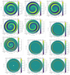Fig. 1. Dimensionless surface density of spiral arms (m = 1) for Model A. The six panels in the upper left corner are the spiral arms for more massive disks (Mdisk/M• = 0.8), and the six panels in the lower right corner are those for less massive disks (Mdisk/M• = 0.2). The values of $\overline{Q}$, Mdisk/M•, and Rout/Rin are marked on the top of each panel. In general, more massive disks have more loosely wound spiral arms (see more details in Sect. 3.2). The eigenvalues (real and imaginary parts) of ω are also provided in each of the panels.

We also present the spiral arms of Model B in Fig. 2 (the corresponding eigenvalues are also provided in Appendix A). In general, the spiral arms of Model B are more loosely wound than those in Model A. Moreover, similarly, the arms in more massive disks are more loosely wound. If $\overline{Q}$ is smaller, the spiral arms wind more tightly. The influence of R_out/R_in on the primary arms in the outer part of the disk is still weak, but the inner part of the disks with larger R_out/R_in show some weak small arms in the less massive disks. More importantly, in comparison with Model A, the spiral arms of Model B are more “banana”-like (see Adams et al. 1989). From the inside out, the arms in Model B do not extend continuously but show several gaps and wiggles. In contrast, this phenomenon is weaker in Model A. The arms in Model A extend outward more continuously.

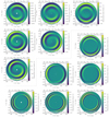Fig. 2. Dimensionless surface density of spiral arms (m = 1) for Model B. Similar to Fig. 1, the six panels in the upper left corner are the spiral arms for more massive disks (Mdisk/M• = 0.8), and the six panels in the lower right corner are those for less massive disks (Mdisk/M• = 0.2). The values of $\overline{Q}$, Mdisk/M•, and Rout/Rin are marked on the top of each panel. The eigenvalues of ω are also provided in each of the panels.

Our goal is to investigate the observational characteristics of the loosely wound spiral arms. We focus on the cases with $(\overline{Q},M_{\mathrm{disk}}/M_{\bullet },R_{\mathrm{out}}/R_{\mathrm{in}})=(2.5,0.8,100)$ and calculate their profiles of emission lines, the velocity-delay maps, and the velocity-resolved lags in Sects. 4.1–4.3.

3.3. Spiral arms with m = 2

We also calculate the two-armed density waves (m = 2). The m = 2 spiral arms of Models A and B with M_disk/M_• = 0.8 and R_out/R_in = 100 are shown in Fig. 3. Similar to m = 1 modes, the m = 2 modes wind more loosely if $\overline{Q}$ is larger. Comparing with the m = 1 modes, the arms in the m = 2 modes can extend inward to smaller radii. The outer parts of the disks tend to be loosely wound, while the inner parts wind more tightly. In comparison with Model A, the pitch angles of the arms in Model B are larger and the “banana” shape of the arms is more significant. In Sect. 4.2, we also present the velocity-delay maps of the m = 2 spiral arms for the cases of $(\overline{Q},M_{\mathrm{disk}}/M_{\bullet },R_{\mathrm{out}}/R_{\mathrm{in}})=(2.5,0.8,100)$.

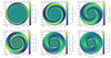Fig. 3. Dimensionless surface density of the spiral arms with m = 2 for Models A and B. The upper three panels are the arm patterns of Model A, and the lower three panels are those of Model B. We only plot the spiral arms with Rout/Rin = 100 as examples.

4. Observational characteristics

4.1. Emission-line profiles

In our models, the surface density distributions are assumed to be power laws (see Sect. 3.1). However, the emissivities of broad emission lines do not necessarily follow the same rules. The locally optimally emitting clouds (LOC) scenario (e.g., Baldwin et al. 1995; Korista et al. 1997) has been successfully applied to investigate and reproduce the observed flux ratios of the prominent broad emission lines (e.g., Korista & Goad 2000; Leighly 2004; Nagao et al. 2006; Marziani et al. 2010; Negrete et al. 2012; Panda et al. 2018). The main concept of the LOC scenario is that, although the BLR gas covers a wide range of physical conditions (e.g., density, ionization parameter), emission lines always tend to emit from their own optimal places (e.g., Baldwin et al. 1995; Korista et al. 1997). Following Paper I, we simply assume that the emission-line emissivity Ξ is a Gaussian function of the ionization parameter U of the BLR gas with the form of

$$\begin{array}{c}\hfill \mathrm{\Xi }\propto \frac{1}{\sqrt{2\pi }{\sigma }_U}{e}^{-{(U-U_{\mathrm{c}})}^2/2{\sigma }_U^2},\end{array}$$(22)

where U_c = U(R = μ_UR_BLR) is the ionization parameter corresponding to the most efficient reprocessing (at the radius of R = μ_UR_BLR), ${\sigma }_U={\stackrel{\sim }{\sigma }}_U\times (U_{0,\max }-U_{0,\min })$ represents the range of efficient reprocessing, U_0, max and U_0, min are the maximum and minimum ionization parameters in the unperturbed disk, and μ_U and ${\stackrel{\sim }{\sigma }}_U$ are two dimensionless parameters. The ionization parameter of the BLR gas is defined as

$$\begin{array}{c}\hfill U=\frac{Q_{\mathrm{H}}}{4\pi R^{2}c{n}_{\mathrm{H}}},\end{array}$$(23)

where Q_H is the number of hydrogen-ionizing photons, n_H = ρ/m_H is the number density, ρ = (σ₀ + σ₁)/2H = (σ₀ + σ₁)Ω/2a₀ is the hydrogen density, and m_H is the mass of hydrogen. The line profile can be expressed as

$$\begin{array}{c}\hfill F_{\ell }(\lambda )={\displaystyle {\int }_{R_{\mathrm{in}}}^{R_{\mathrm{out}}}R\mathrm{d}R{\int }_0^{2\pi }\mathrm{\Xi }g(R,\mathit{\upsilon })\delta [\lambda -{\lambda }_0(1+\frac{\mathit{\upsilon }·{\mathit{n}}_{\mathrm{obs}}}{c})]\mathrm{d}\phi ,}\end{array}$$(24)

where λ₀ is the central wavelength of the emission line, υ(R, φ) is the velocity of the BLR gas, g(R, υ) is the velocity distribution at R, and n_obs is the unit vector pointing from the observer to the source (LOS).

Many RM campaigns have demonstrated that the line widths of rms spectra are different (narrower or broader) from those of the mean spectra (e.g., Peterson et al. 1998; Bentz et al. 2009; Denney et al. 2009; Barth et al. 2013; Fausnaugh et al. 2017; Grier et al. 2012; Du et al. 2018b; De Rosa et al. 2018; Brotherton et al. 2020), which means the responsivity (varying part) of the BLR is different from its mean emissivity. For simplicity, to simulate this phenomenon, we simply assume the responsivity has the same form as Eq. (22) but with a different set of (μ_U, ${\stackrel{\sim }{\sigma }}_U$) rather than taking into account the real photoionization processes in our calculation (hereafter we use Ξ to denote both emissivity and responsivity). Here we investigate two combinations of (μ_U, ${\stackrel{\sim }{\sigma }}_U$) corresponding to the typical cases where rms spectra are narrower or broader (Cases I and II, respectively). The values of μ_U and ${\stackrel{\sim }{\sigma }}_U$ and the maximum dimensionless surface density S_max are listed in Table 2. We select these parameters because on one hand they can demonstrate the line profiles (or velocity-delay maps in the following Sect. 4.2) at different radii, and on the other hand it is easy for us to simulate the mean and rms spectra with different line widths. We set the maximum value of dimensionless surface density S_max to 0.1 and 0.2 for Models A and B, respectively (also in the following Sects. 4.2 and 4.3). It should be noted that the actual values could be larger or smaller than these values. More detailed calculations including photoionization models will be carried out in a separate paper in the future.

4.1.1. Line profiles with m = 1

We present the emission-line profiles of mean (or single-epoch) spectra and rms spectra for the spiral arms of Models A with m = 1, for different azimuthal angles (φ_los) of LOS, in Fig. 4. The disks are rotating counterclockwise. The LOS inclination angle only changes the widths of the emission lines; we fix the inclination angle to θ_los = 30° in our calculation (θ_los = 0° refers to looking at the disks from face-on). The contribution of the sound speed a₀ is also taken into account by adding a macro-turbulence speed in the direction perpendicular to the disk. For each of the Cases I and II, the mock mean and rms spectra are provided as two rows in Fig. 4. As expected, the mean spectra are broader than the rms spectra in Case I, and are relatively narrower in Case II. It is obvious that the line profiles are generally double-peaked because the most efficient emitting region has a ring-like shape (determined by Eq. (22)). The stronger emissivity or responsivity of the spiral arms results in an obvious asymmetry in the line profiles (see Fig. 4). As the azimuthal angle φ_los increases from 0°, the asymmetry of the profiles periodically changes between symmetric, blueward, and redward. For some cases, the weaker peaks almost disappear (e.g., φ_los = 90° in the first row of Case II). In Case II, the asymmetries caused by the spiral arms are more significant because the μ_U parameters are larger and the ${\stackrel{\sim }{\sigma }}_U$ are smaller. More importantly, the asymmetries of the mock mean and rms spectra can be totally different (blueward or redward) even if the LOSs are exactly the same (see e.g., φ_los = 180° in Case II). This implies that the spiral arms can naturally produce differently asymmetric mean and rms spectra without any further special assumptions.

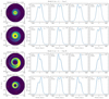Fig. 4. Emission-line profiles of Model A in Cases I and II. The left panel in each row is the Ξ image. The values of (μU, ${\stackrel{\sim }{\sigma }}_U$) and Smax are marked on the top of the Ξ images. The red dotted lines mark the LOS azimuthal angles φlos. The four panels on the right in each row are the line profiles (blue solid lines) corresponding to different φlos. The gray dashed lines are the profiles without spiral arms. The line profiles (mock mean and rms) of the spiral arms for Case I are provided in the upper two rows, and the profiles of Case II are shown in the lower rows.

In Model B, the emissivity or responsivity tends to be distributed over an area covering greater radii (because U ∝ R^3/4 approximately). The emissivities or responsivities of the spiral arms and the corresponding emission-line profiles for Model B in Cases I and II are shown in Fig. 5. The banana-like distributions of the spiral arms in Model B (see Sect. 3.2 and Fig. 2) still make the emission-line profiles significantly asymmetric. Compared with Model A, Model B has less asymmetric line profiles.

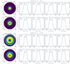Fig. 5. Emission-line profiles of Model B in Cases I and II. The contents of the panels and the meaning of the different lines (solid and dashed) are the same as in Fig. 4.

Some of the mock line profiles in Figs. 4 and 5 are very similar to the observations. We provide a simple comparison between the models and observations in Sect. 5.1.

4.1.2. Line profiles with m = 2

For the spiral arms with m = 2, the profiles of their corresponding emission lines are symmetric and double-peaked. The perturbation σ₁ is identical if φ increases every 180° (m-fold axis-symmetric), meaning that the emissivities on the left and right sides of the LOS (blueshifted and redshifted) are exactly the same. Therefore, the line profiles of the arms with m = 2 have no asymmetry and are the same as the dashed lines in Figs. 4 and 5.

4.2. Velocity-delay maps

Reverberation mapping can be approximated as a linear model, whereby

$$\begin{array}{c}\hfill \mathrm{\Delta }{L}_{\ell }(\upsilon ,t)={\displaystyle {\int }_{-\infty }^{+\infty }\mathrm{\Psi }(\upsilon ,\tau )\mathrm{\Delta }{L}_{\mathrm{c}}(t-\tau )\mathrm{d}\tau ,}\end{array}$$(25)

where Ψ(υ, τ) is the so-called velocity-delay map (or transfer function), ΔL_c(t) is the continuum light curve, and ΔL_ℓ(υ, t) is the variation of the emission-line profile at different epochs (e.g., Blandford & McKee 1982). The velocity-delay map describes how the line profile responds to the varying continuum flux, and is determined by the geometry, kinematics, and emissivity of the gas in the BLR. The velocity-delay map of a simple Keplerian disk is symmetric, and has been calculated numerically and demonstrated in many works (Welsh & Horne 1991; Perez et al. 1992; Horne et al. 2004; Grier et al. 2013, or see Appendix D in Paper I).

The velocity-delay map can be calculated as

$$\begin{array}{c}\hfill \begin{array}{c}\hfill \mathrm{\Psi }(\upsilon ,t)={\displaystyle {\int }_{R_{\mathrm{in}}}^{R_{\mathrm{out}}}R\mathrm{d}R{\int }_0^{2\pi }\mathrm{\Xi }g(R,\mathit{\upsilon })\delta (\upsilon -\mathit{\upsilon }·{\mathit{n}}_{\mathrm{obs}})}\\ \hfill \times \delta [t-\frac{R+\mathit{R}·{\mathit{n}}_{\mathrm{obs}}}{c}]\mathrm{d}\phi .\end{array}\end{array}$$(26)

In the calculation of emission-line profiles, we adopt two sets of parameters (μ_U, ${\stackrel{\sim }{\sigma }}_U$) for each case in Models A and B in order to simulate the mean and rms spectra (Ξ represents emissivity and responsivity, respectively). Strictly speaking, in the calculation of velocity-delay maps, we ought to employ the responsivity implication of Ξ; however, we do not distinguish responsivity and emissivity here because we simply assume that they have the same form mathematically (Gaussian distributions, see Sect. 4.1). The only difference between them is that their (μ_U, ${\stackrel{\sim }{\sigma }}_U$) are not the same. We still calculate the velocity-delay maps using the μ_U and ${\stackrel{\sim }{\sigma }}_U$ in Table 2, and use the nomenclature Ξ in the following discussions. The LOS inclination angle is fixed to θ_los = 30°. A smaller or larger angle will cause the velocity-delay maps to narrow or broaden in their velocity axes.

4.2.1. Velocity-delay maps with m = 1

Similarly to the line profiles, we calculate the velocity-delay maps of Models A and B for different LOS azimuthal angles. The results for both Cases I and II are shown in Figs. 6 and 7. The sound speed has also been taken into account, and so the corresponding velocity-delay maps appear moderately smooth. The general morphologies of the velocity-delay maps are similar to the traditional “bell”-like envelope with a bright “elliptical ring” of a simple Keplerian disk (e.g., Welsh & Horne 1991; Perez et al. 1992; Horne et al. 2004; Grier et al. 2013). However, they are significantly asymmetric and show remarkable subfeatures of bright arcs or strips (indicating strong responses from the arms). The asymmetries of the responses in the velocity-delay maps are consistent with the asymmetries of the line profiles in Figs. 4 and 5.

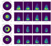Fig. 6. Velocity-delay maps of Model A (m = 1) in Cases I and II. The left panel in each row is the Ξ image. The red dotted lines mark the LOS azimuthal angles φlos. The four panels on the right in each row are the velocity-delay maps corresponding to different φlos.

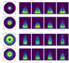Fig. 7. Velocity-delay maps of Model B (m = 1) in Cases I and II. The contents of the panels is the same as in Fig. 6.

In Model A, the contributions from the strong responsivities of the spiral arms appear significant (see Fig. 6). As the azimuthal angle increases from 0° to 270°, the asymmetry and the locations of the arcs and strips in the maps caused by the strong arm responsivities change correspondingly.

In Case II, the spiral-arm patterns are more significant in the Ξ distributions if the strong-response regions are mainly located in larger radii. The bright arcs or strips (the strongest responses) in the velocity-delay maps correspond to the crests of the density waves. For μ_U = 1.20, ${\stackrel{\sim }{\sigma }}_U=0.05$, and φ_los = 270°, the emission-line profile in Fig. 4 is almost symmetric and indistinguishable from that of a simple Keplerian disk. However, the velocity-delay map can break this degeneracy. The subfeatures in the corresponding velocity-delay map are obvious and asymmetrically distributed. In the velocity-delay map of μ_U = 0.60, ${\stackrel{\sim }{\sigma }}_U=0.10$ (or μ_U = 1.00, ${\stackrel{\sim }{\sigma }}_U=0.10$), and φ_los = 90°, there is an arc that starts from blue velocities and extends toward a long time lag. However, the arc does not circle back to the red velocities. It is very interesting that this subfeature is almost the same as that seen in observations of NGC 5548 (incomplete ellipse; see Fig. 3 in Xiao et al. 2018b and Fig. 5 in Horne et al. 2021).

For Model B, the morphologies of the responsivity (Ξ) distributions are more banana-like (bright on one side, and dark on the opposite side). The asymmetries and substructures in the velocity-delay maps are slightly weaker (but still significant) than Model A. The semicircle arcs in Ξ (see Fig. 7) result in strips and arcs overlapped with the original bell-like signatures in the velocity-delay maps. These subfeatures (bright arcs and strips) rotate close-wise along with the increases in LOS azimuthal angle.

4.2.2. Velocity-delay maps with m = 2

As mentioned in Sect. 4.1.2, the line profiles of the spiral arms with m = 2 have no asymmetries and are not different from the profiles of a simple Keplerian disk. However, the velocity-delay maps can break this degeneracy. The maps of the m = 2 arms show significant subfeatures and may be distinguishable in observations. We calculate the corresponding velocity-delay maps for Models A and B with m = 2 (see Figs. 8 and 9). Similarly to Sect. 4.2.1, we adopt $(\overline{Q},M_{\mathrm{disk}}/M_{\bullet },R_{\mathrm{out}}/R_{\mathrm{in}})=(2.5,0.8,100)$. The spiral arms with m = 2 tend to wind loosely in the outer parts of the disks and tightly at the inner radii (see Fig. 3). Compared with the cases of m = 1, the m = 2 arms can extend to radii closer to the center of the disk, and therefore their contributions in the velocity-delay maps are more significant. In addition, Ξ tends to be more banana-like in Model B, which is similar to the cases with m = 1.

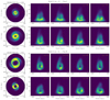Fig. 8. Velocity-delay maps of Model A (m = 2) in Cases I and II. The contents of the panels is the same as in Fig. 6.

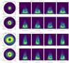Fig. 9. Velocity-delay maps of Model B (m = 2) in Cases I and II. The contents of the panels is the same as in Fig. 9.

The velocity-delay maps of the spiral arms with m = 2 are clearly asymmetric and different from the velocity-delay map of a simple Keplerian disk. The distributions of the strongest responses (bright arcs/strips in Figs. 8 and 9) in the maps change along with the LOS azimuthal angle. For example, for the velocity-delay map of μ_U = 2.00 and ${\stackrel{\sim }{\sigma }}_U=0.05$ in Model A, the strongest responses tend to be in the lower right corner if φ_los = 0° and rotate to the lowest place if φ_los = 90°.

For Model B, the arms in the central parts also contribute strong signals in the maps (see Fig. 9). The maps appear inhomogeneous and have many subfeatures. The lower parts of the maps have multiple layers (similar to lasagna) in Case I of both Model A and B. This is a typical feature in velocity-delay maps if there are a number of arms in the inner radius of the Ξ-map.

4.3. Velocity-resolved lags

Because of the strict requirement for high-quality data, it is not always easy to obtain velocity-delay maps. As a compromise, the velocity-resolved lag analysis is also useful for probing BLR geometry and kinematics, and has been applied in many RM campaigns (e.g., Bentz et al. 2008, 2009; Denney et al. 2009, 2010; Grier et al. 2013; Du et al. 2016b, 2018b; De Rosa et al. 2018; Brotherton et al. 2020; Hu et al. 2021; Lu et al. 2021; Vivian et al. 2022; Bao et al. 2022). We present the velocity-resolved lags for Models A and B in Cases I and II with m = 1 by averaging the velocity-delay maps (Figs. 6 and 7) along their time axes. The results are shown in Fig. 10. The blue lines are the velocity-resolved lags of Model A, and the orange lines are those of Model B. Similarly to the corresponding velocity-delay maps, the velocity-resolved lags are also asymmetric.

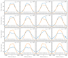Fig. 10. Velocity-resolved lags. The blue and orange lines correspond to Models A and B (m = 1), respectively. The reprocessing coefficients and LOS azimuthal angles are marked in each panel.

Usually, the velocity-resolved lags with shorter (longer) lags in blue velocities and longer (shorter) lags in red velocities tend to be interpreted as outflow (inflow). The velocity-resolved lags, which are generally disk-like (the lags in small velocities are longer than those in high velocities) but show asymmetries to some extent (blue or red lags are shorter, and are referred to as disk-like but with asymmetry hereafter), are sometimes explained by Keplerian disks with some inflowing or outflowing velocities (e.g., De Rosa et al. 2018; Lu et al. 2019). However, the results shown in Fig. 10 demonstrate that spiral arms can also produce disk-like velocity-resolved lags but with some asymmetries. This implies that the velocity-resolved lags are sometimes not sufficient for the diagnostic of BLR geometry and kinematics, because they still have degeneracy.

Here, we do not plot the velocity-resolved lags for the m = 2 arms. The arms are m-fold axis-symmetric, and therefore their velocity-resolved lags do not have any asymmetry.

5. Discussions

5.1. Emission-line profiles: A simple comparison between models and observations

In observations, the asymmetries of the emission-line profiles in single-epoch spectra have been reported for a number of Seyfert galaxies and quasars since the 1970s (e.g., Osterbrock 1977; De Robertis 1985; Boroson & Green 1992; Marziani et al. 1996, 2003; Brotherton 1996). The asymmetries include the single-peaked profile whose peak is blueshifted or redshifted, the single-peaked profile that has a stronger blue or red wing but a zero-velocity peak, and the double-peaked profile with a stronger blue or red peak. Some models have been proposed to explain the asymmetries of the emission-line profiles in AGNs. Capriotti et al. (1979, 1981) suggested that the optically thick clouds with inflow or outflow velocities in BLRs can produce asymmetric broad emission lines. Ferland et al. (1979) also proposed that a stronger red wing can be explained by the self absorption of the line radiation in an expanding BLR with optically thick clouds. Raine & Smith (1981) established a disk BLR model illuminated by the scattered radiation from the wind, which can yield slight asymmetric line profiles. The double-peaked asymmetric line profiles can be explained by a relativistic Keplerian disk (Chen et al. 1989). Eracleous et al. (1995) interpreted the double-peaked profiles whose red peak is stronger than the blue one as an elliptical BLR disk, which is contrary to the prediction of a relativistic disk. More recently, Storchi-Bergmann et al. (2003, 2017), and Schimoia et al. (2012) proposed that the spiral arms can explain the double-peaked, asymmetric line profiles and their variations, but this was based on mathematical models that presume the analytical forms of the perturbation rather than a physical model such as in the present paper. In addition, the asymmetries of the line profiles can also be attributed to supermassive binary black holes (e.g., Shen & Loeb 2010; Bon et al. 2012; Li et al. 2016; Ji et al. 2021). The physical model of density waves in this paper can produce the double-peaked and asymmetric line profiles shown in Figs. 4 and 5.

More importantly, if the emissivity distributions of the mean and rms spectra are different (this is always the case in observations), the line profiles of the mean and rms spectra in the BLR spiral-arm models of the present papers can naturally produce very different asymmetries. For instance, the mean spectrum has a blue asymmetry but the rms spectrum has a red asymmetry, or one is generally symmetric but the other is significantly asymmetric (see Figs. 4 and 5). In observations, the mean and rms spectra in many objects have very different line asymmetries (e.g., Mrk 202, Mrk 704, 3C 120, NGC 2617, NGC 3227, NGC 3516, NGC 4151, NGC 4593, NGC 5548, NGC 6814,SBS 1518+693 in Peterson et al. 1998; Bentz et al. 2009; Denney et al. 2009; Grier et al. 2012; Barth et al. 2013; Fausnaugh et al. 2017; Du et al. 2018b; De Rosa et al. 2018; Brotherton et al. 2020). The BLR model with spiral arms is a very promising mechanism that can easily explain the differences in the line profiles between the mean and rms spectra of RM campaigns.

Fitting the observed mean or rms line profiles with the present model is beyond the scope of this paper. We simply select some line profiles from our Models A and B (without any fine-tuning), and then discover that it is easy to find some observed rms spectra that have almost the same profiles as these models. Some simple comparisons between the profiles of models and observations are provided in Fig. 11.

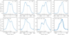Fig. 11. Some examples of the comparisons between the emission-line profiles generated from the models and observed in RM campaigns. The upper panels are the models, and the lower are the observed rms spectra extracted directly from the references marked in the lower left corners. The models, the parameters (μU, ${\stackrel{\sim }{\sigma }}_U$, and Smax), and the LOS azimuthal angles are marked in the lower left and upper right corners in the upper panels. The names of the objects are provided in the lower panels.

The vertical radiation pressure may drive some gas flow from the disk surface (e.g., Wang et al. 2012; Czerny et al. 2017; Elvis 2017). This potential gas flow may contribute some velocity broadening or extra blueshift asymmetry to the line profiles (may also influence the velocity-resolved lags and velocity-delay maps). This effect will be considered in more detail in the future.

5.2. Velocity-delay map of NGC 5548 and implications for BLR spiral arms

The high-quality velocity-delay maps of the Hβ-emitting region in NGC 5548 have been successfully reconstructed by the maximum entropy method in two RM campaigns in 2014 and 2015, and are presented in Horne et al. (2021) and Xiao et al. (2018b), respectively. The two maps in 2014 and 2015 are very similar, and both of them show traditional bell-like envelopes with bright elliptical rings, which are a typical signature of a simple Keplerian disk. However, the responses at the red velocities (∼2000 km s⁻¹) and long time lags (∼30 days) are weaker than the other parts in both of the two maps (Horne et al. 2021 refers to this as an incomplete ellipse). Xiao et al. (2018b) suggested that this weak response is due to the inhomogeneity of the outer part of the BLR in NGC 5548. In addition, Horne et al. (2021) presents a helical “barber-pole” pattern in the C IV line of NGC 5548, which also implies the potential existence of some azimuthal structures in the BLR.

The spiral arms stimulated from the self-gravity instabilities are probably the physical origin of the weak response (incomplete ellipse) in the velocity-delay map of NGC 5548. The velocity-delay map produced by Model A with μ_U = 0.60, ${\stackrel{\sim }{\sigma }}_U=0.10$ (or μ_U = 1.00, ${\stackrel{\sim }{\sigma }}_U=0.10$), and φ_los = 90° (shown in Fig. 6) has a similar weak response at red velocities and long time lags (incomplete ellipse). We will carry out detailed fitting to the velocity-delay map of NGC 5548 with the spiral-arm model in a separate paper in the future.

5.3. Changes of emission-line profiles and velocity-resolved lags: Arm rotation, changes in emissivity or responsivity, or instabilities of spiral arms

The real part of eigenvalues ω represents the rotation speed of the spiral arms, and depends on M_disk/M_•, $\overline{Q}$, R_out/R_in, and the inner and outer radii. We provide the values of ω in Figs. 1–3. The timescale 2π/ω over which the arms rotate 360° spans from ∼70 years to ∼110 years for the cases with M_disk/M_• = 0.8 in the present paper. However, as shown in Figs. 4, 5, and 10, the emission-line profiles and the velocity-resolved lags (or even velocity-delay maps) can vary significantly if φ_los changes by 90°. Thus, observers will discover that the emission-line profiles and the velocity-resolved lags (or even velocity-delay maps) change significantly in ∼20 − 30 years if the BLR has similar parameters to those adopted here (M_• = 10⁸ M_⊙ and $\dot{\mathcal{M}}=1.0$). Even if the parameters are different and the spiral arms prefer a different mode (see Appendix A), the timescale can decrease further (to less than ∼10 years). From Appendix A, the real part of ω is generally on the order of ${(G{M}_{•}/R_{\text{out}}^3)}^{1/2}$ (or larger than ${(G{M}_{•}/R_{\text{out}}^3)}^{1/2}$ by factors of a few), where ${(G{M}_{•}/R_{\text{out}}^3)}^{1/2}$ is the Keplerian rotation frequency at the outer radius of the disk. The rotation timescale may be roughly $\propto {(L^{3/2}/M_{\bullet })}^{1/2}\propto M_{\bullet }^{1/4}{\dot{\mathcal{M}}}^{3/4}$. Therefore, the rotation timescale may be smaller if the accretion rate and BH mass are smaller.

In observations, the emission-line profiles (mean or rms) and the velocity-resolved time lags have shown significant changes between two campaigns several to ten years apart. For instance, the line profile in the rms spectrum of NGC 3227 was symmetric and double-peaked in 2007 (Denney et al. 2009), but became asymmetric and single-peaked (the peak is redshifted) with a strong blue wing in 2017 (Brotherton et al. 2020); its velocity-resolved lags changed from shorter in the blue velocities and longer in the red ones to vice versa from 2007 to 2017 (Denney et al. 2009; Brotherton et al. 2020). The velocity-resolved lags of NGC 3516 changed from longer in the blue and shorter in the red to vice versa (to some extent) from 2007 to 2012 (Denney et al. 2009; De Rosa et al. 2018), and changed back in 2018–2019 (Feng et al. 2021). Considering their smaller black hole masses, the timescales of these changes are generally consistent with the rotation timescale of the density waves. The spiral arms in BLRs are probably a very natural explanation for such quick changes. In particular, some of the periodic variations in the line profiles (or in the velocity-resolved lags or velocity-delay maps in future observations) can probably be explained by the spiral arms. Future detailed modeling will reveal the surface densities and azimuthal angles of the spiral arms in those objects.

Furthermore, if the continuum luminosities vary, the emissivity or responsivity distributions may change accordingly because of the photoionization physics (e.g., μ_U, ${\stackrel{\sim }{\sigma }}_U$ may be different). In this case, the line profiles, velocity-resolved lags, and velocity-delay maps can show significant changes within even shorter timescales (light-traveling timescale). Therefore, it must be crucial to monitor an object (especially the ones with large variations, or even changing-look AGNs) repeatedly in different luminosity states.

Finally, the instabilities of spiral arms could also be an origin of the short timescales of the changes in the emission-line profiles (single-epoch, mean, or rms) and the velocity-resolved lags. The growth rates can be comparable to the Keplerian timescales at the outer radii, especially for Model A (for Model B, the growth timescale is longer than the Keplerian timescale by factors of a few to ten; see Figs. A.1–A.3 in Appendix A), which means that the timescales of the instabilities for spiral arms can be relatively short. As mentioned above, the line profiles and the velocity-resolved lags can change within a period as short as ≲-pagination10 years (e.g., NGC 3227, NGC 3516). In addition, the line profiles (single-epoch, mean, or rms spectra) of some objects (e.g., Mrk 6 in Doroshenko et al. 2012 and Du et al. 2018b; 3C 390.3 in Sergeev 2020 and Du et al. 2018b) also show obvious changes, but over longer timescales of ∼20 − 30 years. The instabilities of spiral arms could also be a possible explanation for those changes. However, it should be noted that the growth timescale is still significantly longer than the rotation timescale (see Figs. A.1–A.3), and therefore the changes caused by the instabilities of arms may be slower than those caused by the rotation. Moreover, the changes caused by the instabilities should be more chaotic, but those caused by the rotation should be ordered and probably periodic.

5.4. Observational tests in the future

As shown above, directly searching the spiral-arm signatures from the velocity-delay maps and emission-line profiles in RM campaigns is a very promising way to identify the spiral arms in BLRs. Recently, the trend in RM campaigns is to focus on a specific subclass of AGNs in order to investigate their unique properties; for example, the “Monitoring AGNs with Hβ Asymmetry” (MAHA) project targets AGNs with asymmetric Hβ emission lines (Du et al. 2018b; Brotherton et al. 2020; Bao et al. 2022). We may identify some BLRs with spiral arms from the velocity-delay maps or emission-line profiles in the MAHA project in the future. In addition, it is also promising to search for candidate spiral-arm BLRs from some spectroscopic samples of AGNs with asymmetric emission-line profiles (e.g., Eracleous et al. 2012).

Furthermore, RM of some AGNs with very large flux variations may be helpful. The velocity-delay maps of the same object at high and low states can probe different radii of its BLR (high state for larger radius and low state for smaller radius), and will provide better constraints on the spiral-arm pattern.

5.5. Roles of parameters Q and M_disk/M_•

In Sect. 3, we show that the spiral arms wind more loosely if the Toomre parameter Q and the mass ratio M_disk/M_• are larger. This phenomenon is easy to understand. The dispersion relation of the gravitational instabilities can be expressed, in its lowest approximation, as (ω − mΩ)² = κ² + (ka₀)² − 2πGσ₀|k|, where k is the wave number (Lin & Lau 1979). The waves are trailing if k < 0. The solution of the dispersion relation is $k=-k_0[1\pm \sqrt{1-Q^2(1-{\nu }^2)}]$, where k₀ = κ²/πGσ₀Q². Considering that M_disk/M_• is proportional to σ₀, the wave number |k| decreases and the wavelength increases (arms wind more loosely) if Q and M_disk/M_• are larger.

5.6. Linear analysis and σ₁/σ₀

As a first step, we adopted the linear analysis to describe the density wave in disk-like BLRs and neglect the viscosity in the present paper for simplicity. The absolute amplitude of σ₁ cannot be directly deduced from Eq. (8) and is freely scalable (the solution of Eq. (18) can be $S_l^{*}$ or $C{S}_l^{*}$ with an arbitrary constant C). In more realistic calculations, the dissipation processes, such as shocks, nonlinear growth of perturbations, or viscous stress, should be taken into account. On the one hand, the dissipation can lead to deposition of the angular momentum carried by a density wave to the disk, which may also induce changes in the surface density of the disk. On the other hand, the absolute amplitude of σ₁ may be determined if the growth of the perturbation becomes saturated by the dissipation processes (e.g., Laughlin & Rozyczka 1996; Laughlin et al. 1997). These effects are not included in the equations of motion presented here (Eqs. (5) and (6)) or in the normal mode matrix equation (Eq. (18)), and will be considered further in the future.

5.7. Accretion driven by spiral arms

The dimensionless accretion rate $\dot{\mathcal{M}}$ is only used to determine the continuum luminosity, hence the inner and outer radii, and the appropriate reference parameters for Ξ in Table 2. We mainly focus on the spiral arms in BLRs, which typically span from 10³R_g to 10⁵R_g. The UV/optical continuum luminosity comes from the more inner accretion disk (≲10³R_g), which could be in the Shakura & Sunyaev regime (Shakura & Sunyaev 1973). Discussing the angular momentum transfer in detail is beyond the scope of this paper. However, we can roughly evaluate whether or not the accretion rate driven by the spiral structures in these regions is sufficient for the accretion in the inner disk.

In a viscous thin disk with quasi-Keplerian rotation, the radial velocity induced by a viscosity ν_vis (Lynden-Bell & Pringle 1974) can be expressed as

$$\begin{array}{c}\hfill u={\left[{\sigma }_{0}R\frac{\partial \mathrm{\Omega }{R}^2}{\partial R}\right]}^{-1}\frac{\partial }{\partial R}\left[{\sigma }_0{\nu }_{\mathrm{vis}}{R}^3\frac{\partial \mathrm{\Omega }}{\partial R}\right]\sim \alpha a_0\frac{H}{R},\end{array}$$(27)

where ν_vis = αa₀H is an effective “alpha”-type viscosity, α is the viscosity parameter, and H is the thickness of the disk. The mass-accretion rate can be obtained with Ṁ_∙ = 2πRuσ₀. The global spiral arms may redistribute the disk material and be described in terms of a diffusive process with an effective viscosity α_eff (Laughlin & Rozyczka 1996). α_eff is on the order of 0.01 (especially in the nonlinear regime; see e.g., Laughlin & Bodenheimer 1994; Laughlin & Rozyczka 1996; Lodato & Rice 2005). We checked that, with such a α_eff, the disk properties assumed in the present paper (σ₀, a₀, H, and Ω) can very easily support the accretion with $\dot{\mathcal{M}}\sim$ 1.

5.8. Vertical structures and possible influences

Given the sound speed a₀ and rotation curve Ω, the thickness of the disk is H/R ∼ R^1/8 and H/R ∼ R^1/4 for Models A and B, respectively. This means that the geometry of the disk is “bowl-shaped” (concave, see Starkey et al. 2023). Such a geometry can enable the disk to be illuminated by the ionizing photons from the inner region.

With surface density (σ₁) variations, the disk thickness is also likely to modulate. The wave crest of the arm may be more strongly irradiated by the ionizing photons because it protrudes from the disk surface. On the contrary, the wave trough may be more weakly irradiated. Therefore, the asymmetries of the line profiles and velocity-resolved lags could be stronger, as could the subfeatures in the velocity-delay maps. A sophisticated treatment of the vertical structures and of the corresponding influences on the observation is needed in the future.

5.9. Boundary conditions

In this paper, we adopt the same boundary conditions as in Adams et al. (1989) for simplicity. Noh et al. (1991) and Chen et al. (2021) investigated the influence of boundary conditions on the pitch angles, pattern speeds, and growth rates of spiral arms in protoplanetary disks. These authors tried reflecting and transmitting boundaries in addition to the boundary conditions of Adams et al. (1989), and found that the boundary conditions mainly influence the growth rates but have little effect on the pitch angles and pattern speeds of the arms (the differences are ≲-pagination10% for different boundary conditions). Noh et al. (1991) and Chen et al. (2021) indicate that adopting the boundary conditions of Adams et al. (1989) is sufficient to demonstrate the general reverberation properties of the BLR arms. In the future, the boundary conditions may be revised by comparing the models with the real observations.

6. Summary

There is growing evidence that some BLRs are inhomogeneous and have substructures. The radii of BLRs measured by RM are consistent with the self-gravitating regions of accretion disks, which implies that the spiral arms excited by the gravitational instabilities may at least exist in the disk-like BLRs. In this paper, we calculate the surface densities of the spiral arms in BLRs for two typical configurations (referred to here as Models A and B) with different parameters using the density wave theory. We find that more massive disks (larger disk-to-SMBH mass ratios) with larger Toomre parameters tend to have more loosely wound arms (more significant in observations). In comparison with Model A, the spiral arms of Model B are more “banana”-like.

We present the emission-line profiles, velocity-delay maps, and velocity-resolved lags for the cases of loosely wound spiral arms (in more massive BLR disks). For m = 1 spiral arms, the emission-line profiles and velocity-resolved lags show significant asymmetries, and the velocity-delay maps are asymmetric and show complex substructures (bright arcs or strips). For m = 2 spiral arms, the emission-line profiles and velocity-resolved lags are symmetric, but the velocity-delay maps are also asymmetric and show complex substructures. The spiral arms in BLRs can easily explain some of the phenomena seen in observations:

• For the same object, the mean and rms spectra in RM observations can have very different asymmetries. The rms spectra always have different widths compared to the mean spectra in RM campaigns, which implies that the emissivities and responsivities of the invariable and variable parts in BLRs are different. Considering the different emissivities and responsivities, the calculations in the present paper show that the spiral arms in BLRs can naturally produce differently asymmetric line profiles in the mean and rms spectra of the same object without any further special assumptions.

• Our models can generate almost the same emission-line profiles as those seen in observations (rms spectra).

• The spiral arms in the disk-like BLRs can produce complex features such as bright arcs or strips, and are probably the physical origin of the relatively weak response region (incomplete ellipse) in the velocity-delay map of NGC 5548.

• The timescale over which the spiral arms rotate φ_los ∼ 90° (which can significantly change the line profiles or velocity-resolved lags) can be as short as ≲-pagination10 years. The rotation of the spiral arms can explain the rapid changes of the asymmetries in the emission-line profiles, the velocity-resolved lags, or even velocity-delay maps between RM campaigns several to ten years apart. Furthermore, some of the periodic variations in the line profiles (or in the velocity-resolved lags or velocity-delay maps in future observations) can probably be explained by the rotation of the BLR spiral arms.

• The line profiles, velocity-resolved lags, and velocity-delay maps can show significant changes within short timescales (light-traveling timescale) if the continuum varies significantly.

We show the emission-line profiles, velocity-delay maps, and velocity-resolved lags calculated from the model of spiral arms in BLRs in this paper. Sophisticated fitting of observations to spiral-arm models will help to reveal the detailed geometry and kinematics of BLRs in the future.

Acknowledgments

We thank the anonymous referee for the useful comments that improved the manuscript. We acknowledge the support by National Key R&D Program of China (grants 2021YFA1600404, 2016YFA0400701), the support by the National Science Foundation of China through grants NSFC-12022301, -11991051, -11991054, -11873048, -11833008, by Grant No. QYZDJ-SSW-SLH007 from the Key Research Program of Frontier Sciences, Chinese Academy of Sciences (CAS), by the Strategic Priority Research Program of CAS grant No.XDB23010400, and by the International Partnership Program of CAS, Grant No.113111KYSB20200014.

References

Appendix A: Eigenvalues

A.1. Eigenvalues of Models A and B with m = 1

Here we present the eigenvalues of Models A and B with m = 1 in Figures A.1 and A.2. For each set of parameters, there is more than one eigenvalue and more than one solution (mode). The excitation and the evolution of the modes (which mode will finally dominate) are not fully understood (Bertin et al. 1989). We adopt the mode that has the lowest order (with significant growth rate), because they will span the largest radial range and can grow at a relatively high rate (e.g., Adams et al. 1989; Chen et al. 2021). For consistency, we select the same mode for the same disk-to-SMBH mass ratio (M_disk/M_•) in order to demonstrate how the spiral-arm pattern evolves if the other parameters change, but have checked that it does not change the main conclusions in the present paper if we adopt the other nearby mode. For instance, the lowest mode becomes significant if M_disk/M_• = 0.8, $\overline{Q}=1.5$, and R_out/R_in = 20 in Model A (see Figure A.1). We select the mode with the highest growth rate rather than the lowest mode (see Figure A.1). For Model B, the lowest modes do not have the highest growth rate. We adopt the lowest mode with significant growth rate (also keep selecting the same mode for the same disk-to-SMBH mass ratio).

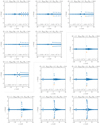Fig. A.1. Eigenvalues of the spiral arms (m = 1) for Model A. The real and imaginary parts of ω are both in units of ${(G{M}_{•}/R_{\text{out}}^3)}^{1/2}$. The six panels in the upper left corner are the eigenvalues for more massive disks (Mdisk/M• = 0.8), and the six panels in the lower right corner are those for less massive disks (Mdisk/M• = 0.2). The values of $\overline{Q}$, Mdisk/M•, and Rout/Rin are marked on the top of each panel. The eigenvalue adopted in the present paper is marked in orange in each panel, and its value is also provided in the same panel.

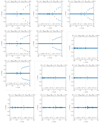Fig. A.2. Eigenvalues of the spiral arms (m = 1) for Model B. Similar to Figure A.1, the real and imaginary parts of ω are both in units of ${(G{M}_{•}/R_{\text{out}}^3)}^{1/2}$. The six panels in upper left corner are the eigenvalues for more massive disks (Mdisk/M• = 0.8), and the six panels in lower right corner are those for less massive disks (Mdisk/M• = 0.2). The values of $\overline{Q}$, Mdisk/M•, and Rout/Rin are marked on the top of each panel. The eigenvalue adopted in the present paper is marked in orange in each panel, and its value is also provided in the same panel.

A.2. Eigenvalues of Models A and B with m = 2

The eigenvalues of Models A and B with m = 2 are shown in Figure A.3. Similarly, we tend to select the lowest mode with significant growth rate.

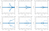Fig. A.3. Eigenvalues of the spiral arms (m = 2) for Models A and B. The real and imaginary parts of ω are both in units of ${(G{M}_{•}/R_{\text{out}}^3)}^{1/2}$. The values of $\overline{Q}$, Mdisk/M•, and Rout/Rin are marked on the top of each panel. The eigenvalue adopted in the present paper is marked in orange in each panel, and its value is also provided in the same panel.

Appendix B: Matrixes in Numerical Method

The details of the numerical method for solving the governing integro-differential equation (Eqn 8) are provided in Adams et al. (1989). However, the coefficients in the matrixes 𝒲⁽⁰⁾, 𝒲⁽¹⁾, 𝒲⁽²⁾, 𝒲⁽³⁾, 𝒲⁽⁴⁾, 𝒲⁽⁵⁾ regrouped from 𝒲_ik are not provided (see Eqn B12 in Adams et al. 1989). In this section, we demonstrate the coefficients of these matrixes. The same nomenclatures as Adams et al. (1989) are adopted here, except the radius, the mass of central object, and the mass of disk are R, M_•, M_disk in the present paper and r, M_*, M_D in Adams et al. (1989), respectively. The matrixes 𝒲⁽⁰⁾, 𝒲⁽¹⁾, 𝒲⁽²⁾, 𝒲⁽³⁾, 𝒲⁽⁴⁾, 𝒲⁽⁵⁾ can be expressed as

$$\begin{array}{c}\hfill \begin{array}{cc}\hfill {\mathcal{W}}^{(0)}& ={\mathcal{F}}^{(0)},\hfill \\ \hfill {\mathcal{W}}^{(1)}& ={\mathcal{F}}^{(1)},\hfill \\ \hfill {\mathcal{W}}^{(2)}& ={\mathcal{F}}^{(2)}+{\mathcal{G}}^{(0)},\hfill \\ \hfill {\mathcal{W}}^{(3)}& ={\mathcal{F}}^{(3)}+{\mathcal{G}}^{(1)},\hfill \\ \hfill {\mathcal{W}}^{(4)}& =-C_2^{(4)}\frac{{\kappa }^{2}R}{2\pi G{\sigma }_0}{\delta }_{\mathit{ik}}+{\mathcal{G}}^{(2)},\hfill \\ \hfill {\mathcal{W}}^{(5)}& =-C_2^{(5)}\frac{{\kappa }^{2}R}{2\pi G{\sigma }_0}{\delta }_{\mathit{ik}}+{\mathcal{G}}^{(3)},\hfill \end{array}\end{array}$$(B.1)

where

$$\begin{array}{c}\hfill \begin{array}{c}\hfill {\mathcal{F}}^{(n)}=\{C_n{\mathcal{D}}_{\mathit{ij}}^{(2)}+[C_A^{(n)}+C_n[2(1-p)-1]]{\mathcal{D}}_{\mathit{ij}}^{(1)}\\ \hfill +[C_B^{(n)}+C_A^{(n)}(1-p)+C_{n}p(p-1)]{\delta }_{\mathit{ij}}\}{\mathcal{I}}_{\mathit{jk}}\\ \hfill +\frac{1}{\mathrm{\Sigma }R}\{C_n{\mathcal{D}}_{\mathit{ik}}^{(2)}+[C_A^{(n)}-C_n(2q+1)]{\mathcal{D}}_{\mathit{ik}}^{(1)}\\ \hfill +[C_B^{(n)}-C_A^{(n)}q+C_{n}q(q+1)]{\delta }_{\mathit{ik}}\}\\ \hfill -C_2^{(n)}\frac{{\kappa }^{2}R}{2\pi G{\sigma }_0}{\delta }_{\mathit{ik}},n=0,1,2,3,\end{array}\end{array}$$(B.2)

and

$$\begin{array}{c}\hfill {\mathcal{G}}^{(n)}={\delta }_{1m}(C_A^{(n)}+C_B^{(n)})\frac{R^3}{2G(M_{\bullet }+M_{\mathrm{disk}})}{\mathcal{J}}_{\mathit{ik}},n=0,1,2,3.\end{array}$$(B.3)

${\mathcal{D}}_{\mathit{ij}}^{(1)}$ and ${\mathcal{D}}_{\mathit{ij}}^{(2)}$ are the first- and second-order derivatives expressed in matrix form, see Eqn (B4a) and (B4b) in Adams et al. (1989). ℐ_jk and 𝒥_ik are two matrixes that perform integrals, see also the appendix in Adams et al. (1989). The coefficients in Eqn (B.1), (B.2), and (B.3) are

$$\begin{array}{c}\hfill \begin{array}{cc}\hfill C_0& =\frac{m^3{\mathrm{\Omega }}^3-m\mathrm{\Omega }{\kappa }^2}{{\kappa }^3},\hfill \\ \hfill C_1& =\frac{{\kappa }^2-3m^2{\mathrm{\Omega }}^2}{{\kappa }^3},\hfill \\ \hfill C_2& =\frac{3m\mathrm{\Omega }}{{\kappa }^3},\hfill \\ \hfill C_3& =-\frac{1}{{\kappa }^3},\hfill \end{array}\end{array}$$(B.4)

$$\begin{array}{c}\hfill \begin{array}{cc}\hfill C_A^{(0)}& =C_0{\mathcal{D}}_{\mathit{ij}}^{(1)}{[log({\sigma }_{0}R)]}_j+\frac{m\mathrm{\Omega }}{{\kappa }^3}{\mathcal{D}}_{\mathit{ij}}^{(1)}{({\kappa }^2)}_j-\frac{2m^3{\mathrm{\Omega }}^2}{{\kappa }^3}{\mathcal{D}}_{\mathit{ij}}^{(1)}{\mathrm{\Omega }}_j,\hfill \\ \hfill C_A^{(1)}& =C_1{\mathcal{D}}_{\mathit{ij}}^{(1)}{[log({\sigma }_{0}R)]}_j-\frac{1}{{\kappa }^3}{\mathcal{D}}_{\mathit{ij}}^{(1)}{({\kappa }^2)}_j+\frac{4m^2\mathrm{\Omega }}{{\kappa }^3}{\mathcal{D}}_{\mathit{ij}}^{(1)}{\mathrm{\Omega }}_j,\hfill \\ \hfill C_A^{(2)}& =C_2{\mathcal{D}}_{\mathit{ij}}^{(1)}{[log({\sigma }_{0}R)]}_j-\frac{2m}{{\kappa }^3}{\mathcal{D}}_{\mathit{ij}}^{(1)}{\mathrm{\Omega }}_j,\hfill \\ \hfill C_A^{(3)}& =C_3{\mathcal{D}}_{\mathit{ij}}^{(1)}{[log({\sigma }_{0}R)]}_j,\hfill \end{array}\end{array}$$(B.5)

$$\begin{array}{c}\hfill \begin{array}{cc}\hfill C_B^{(0)}& =-m^2{C}_0-\frac{4m^3{\mathrm{\Omega }}^2}{{\kappa }^3}{\mathcal{D}}_{\mathit{ij}}^{(1)}{\mathrm{\Omega }}_j+\frac{4m^3{\mathrm{\Omega }}^3}{{\kappa }^4}{\mathcal{D}}_{\mathit{ij}}^{(1)}{\kappa }_j\hfill \\ \hfill & +\frac{2m\mathrm{\Omega }}{{\kappa }^3}({\kappa }^2-m^2{\mathrm{\Omega }}^2){\mathcal{D}}_{\mathit{ij}}^{(1)}{(log\frac{{\kappa }^2}{\mathrm{\Omega }{\sigma }_0})}_j,\hfill \\ \hfill C_B^{(1)}& =-m^2{C}_1+\frac{4m^2\mathrm{\Omega }}{{\kappa }^3}{\mathcal{D}}_{\mathit{ij}}^{(1)}{\mathrm{\Omega }}_j-\frac{8m^2{\mathrm{\Omega }}^2}{{\kappa }^4}{\mathcal{D}}_{\mathit{ij}}^{(1)}{\kappa }_j\hfill \\ \hfill & +\frac{4m^2{\mathrm{\Omega }}^2}{{\kappa }^3}{\mathcal{D}}_{\mathit{ij}}^{(1)}{(log\frac{{\kappa }^2}{\mathrm{\Omega }{\sigma }_0})}_j,\hfill \\ \hfill C_B^{(2)}& =-m^2{C}_2+\frac{4m\mathrm{\Omega }}{{\kappa }^4}{\mathcal{D}}_{\mathit{ij}}^{(1)}{\kappa }_j-\frac{2m\mathrm{\Omega }}{{\kappa }^3}{\mathcal{D}}_{\mathit{ij}}^{(1)}{(log\frac{{\kappa }^2}{\mathrm{\Omega }{\sigma }_0})}_j,\hfill \\ \hfill C_B^{(3)}& =-m^2{C}_3,\hfill \end{array}\end{array}$$(B.6)

and

$$\begin{array}{c}\hfill \begin{array}{cc}\hfill C_2^{(0)}& =-\frac{m\mathrm{\Omega }}{\kappa }+\frac{2m^3{\mathrm{\Omega }}^3}{{\kappa }^3}-\frac{m^5{\mathrm{\Omega }}^5}{{\kappa }^5},\hfill \\ \hfill C_2^{(1)}& =\frac{1}{\kappa }-\frac{6m^2{\mathrm{\Omega }}^2}{{\kappa }^3}+\frac{5m^4{\mathrm{\Omega }}^4}{{\kappa }^5},\hfill \\ \hfill C_2^{(2)}& =\frac{6m\mathrm{\Omega }}{{\kappa }^3}-\frac{10m^3{\mathrm{\Omega }}^3}{{\kappa }^5},\hfill \\ \hfill C_2^{(3)}& =-\frac{2}{{\kappa }^3}+\frac{10m^2{\mathrm{\Omega }}^2}{{\kappa }^5},\hfill \\ \hfill C_2^{(4)}& =-\frac{5m\mathrm{\Omega }}{{\kappa }^5},\hfill \\ \hfill C_2^{(5)}& =\frac{1}{{\kappa }^5}.\hfill \end{array}\end{array}$$(B.7)

The first and last rows of the matrixes 𝒲⁽⁰⁾ to 𝒲⁽⁵⁾ are determined by the boundary conditions, and only have the terms of 0 to 3 orders. The inner boundary conditions are

$$\begin{array}{c}\hfill \begin{array}{cc}\hfill {\mathcal{W}}_{1k}^{(0)}& =[-m\mathrm{\Omega }{\mathcal{D}}_{1j}^{(1)}+(p-3)m\mathrm{\Omega }{\delta }_{1j}]{\mathcal{I}}_{\mathit{jk}}\hfill \\ \hfill & +\frac{1}{\mathrm{\Sigma }R}[-m\mathrm{\Omega }{\mathcal{D}}_{1k}^{(1)}+(q-2)m\mathrm{\Omega }{\delta }_{1k}],\hfill \\ \hfill {\mathcal{W}}_{1k}^{(1)}& =[{\mathcal{D}}_{1j}^{(1)}+(1-p){\delta }_{1j}]{\mathcal{I}}_{\mathit{jk}}+\frac{1}{\mathrm{\Sigma }R}({\mathcal{D}}_{1k}^{(1)}-q{\delta }_{1k}),\hfill \\ \hfill {\mathcal{W}}_{1k}^{(2)}& =-\frac{3{\delta }_{1m}\mathrm{\Omega }{R}^3}{2G(M_{\bullet }+M_{\mathrm{disk}})}{\mathcal{J}}_{1k},\hfill \\ \hfill {\mathcal{W}}_{1k}^{(3)}& =\frac{{\delta }_{1m}{R}^3}{2G(M_{\bullet }+M_{\mathrm{disk}})}{\mathcal{J}}_{1k}.\hfill \end{array}\end{array}$$(B.8)

The outer boundary conditions are

$$\begin{array}{c}\hfill \begin{array}{cc}\hfill {\mathcal{W}}_{\mathit{Nk}}^{(0)}& =[-m\mathrm{\Omega }{\mathcal{D}}_{\mathit{Nj}}^{(1)}+(p-3)m\mathrm{\Omega }{\delta }_{\mathit{Nj}}]{\mathcal{I}}_{\mathit{jk}}\hfill \\ \hfill & +\frac{1}{\mathrm{\Sigma }R}[-m\mathrm{\Omega }{\mathcal{D}}_{\mathit{Nk}}^{(1)}+(q-2)m\mathrm{\Omega }{\delta }_{\mathit{Nk}}]+C_0\frac{{\kappa }^{3}R}{2\pi G{\sigma }_{0}p}{\delta }_{\mathit{Nk}},\hfill \\ \hfill {\mathcal{W}}_{\mathit{Nk}}^{(1)}& =[{\mathcal{D}}_{\mathit{Nj}}^{(1)}+(1-p){\delta }_{\mathit{Nj}}]{\mathcal{I}}_{\mathit{jk}}+\frac{1}{\mathrm{\Sigma }R}({\mathcal{D}}_{\mathit{Nk}}^{(1)}-q{\delta }_{\mathit{Nk}})+C_1\frac{{\kappa }^{3}R}{2\pi G{\sigma }_{0}p}{\delta }_{\mathit{Nk}},\hfill \\ \hfill {\mathcal{W}}_{\mathit{Nk}}^{(2)}& =C_2\frac{{\kappa }^{3}R}{2\pi G{\sigma }_{0}p}{\delta }_{\mathit{Nk}}-\frac{3{\delta }_{1m}\mathrm{\Omega }{R}^3}{2G(M_{\bullet }+M_{\mathrm{disk}})}{\mathcal{J}}_{\mathit{Nk}},\hfill \\ \hfill {\mathcal{W}}_{\mathit{Nk}}^{(3)}& =C_3\frac{{\kappa }^{3}R}{2\pi G{\sigma }_{0}p}{\delta }_{\mathit{Nk}}+\frac{{\delta }_{1m}{R}^3}{2G(M_{\bullet }+M_{\mathrm{disk}})}{\mathcal{J}}_{\mathit{Nk}}.\hfill \end{array}\end{array}$$(B.9)

All Tables

All Figures

Fig. 1. Dimensionless surface density of spiral arms (m = 1) for Model A. The six panels in the upper left corner are the spiral arms for more massive disks (Mdisk/M• = 0.8), and the six panels in the lower right corner are those for less massive disks (Mdisk/M• = 0.2). The values of $\overline{Q}$, Mdisk/M•, and Rout/Rin are marked on the top of each panel. In general, more massive disks have more loosely wound spiral arms (see more details in Sect. 3.2). The eigenvalues (real and imaginary parts) of ω are also provided in each of the panels.

In the text

Fig. 2. Dimensionless surface density of spiral arms (m = 1) for Model B. Similar to Fig. 1, the six panels in the upper left corner are the spiral arms for more massive disks (Mdisk/M• = 0.8), and the six panels in the lower right corner are those for less massive disks (Mdisk/M• = 0.2). The values of $\overline{Q}$, Mdisk/M•, and Rout/Rin are marked on the top of each panel. The eigenvalues of ω are also provided in each of the panels.

In the text

	Fig. 3. Dimensionless surface density of the spiral arms with m = 2 for Models A and B. The upper three panels are the arm patterns of Model A, and the lower three panels are those of Model B. We only plot the spiral arms with Rout/Rin = 100 as examples.
In the text

Fig. 4. Emission-line profiles of Model A in Cases I and II. The left panel in each row is the Ξ image. The values of (μU, ${\stackrel{\sim }{\sigma }}_U$) and Smax are marked on the top of the Ξ images. The red dotted lines mark the LOS azimuthal angles φlos. The four panels on the right in each row are the line profiles (blue solid lines) corresponding to different φlos. The gray dashed lines are the profiles without spiral arms. The line profiles (mock mean and rms) of the spiral arms for Case I are provided in the upper two rows, and the profiles of Case II are shown in the lower rows.

In the text

	Fig. 5. Emission-line profiles of Model B in Cases I and II. The contents of the panels and the meaning of the different lines (solid and dashed) are the same as in Fig. 4.
In the text

	Fig. 6. Velocity-delay maps of Model A (m = 1) in Cases I and II. The left panel in each row is the Ξ image. The red dotted lines mark the LOS azimuthal angles φlos. The four panels on the right in each row are the velocity-delay maps corresponding to different φlos.
In the text

	Fig. 7. Velocity-delay maps of Model B (m = 1) in Cases I and II. The contents of the panels is the same as in Fig. 6.
In the text

	Fig. 8. Velocity-delay maps of Model A (m = 2) in Cases I and II. The contents of the panels is the same as in Fig. 6.
In the text

	Fig. 9. Velocity-delay maps of Model B (m = 2) in Cases I and II. The contents of the panels is the same as in Fig. 9.
In the text

	Fig. 10. Velocity-resolved lags. The blue and orange lines correspond to Models A and B (m = 1), respectively. The reprocessing coefficients and LOS azimuthal angles are marked in each panel.
In the text

Fig. 11. Some examples of the comparisons between the emission-line profiles generated from the models and observed in RM campaigns. The upper panels are the models, and the lower are the observed rms spectra extracted directly from the references marked in the lower left corners. The models, the parameters (μU, ${\stackrel{\sim }{\sigma }}_U$, and Smax), and the LOS azimuthal angles are marked in the lower left and upper right corners in the upper panels. The names of the objects are provided in the lower panels.

In the text

Fig. A.1. Eigenvalues of the spiral arms (m = 1) for Model A. The real and imaginary parts of ω are both in units of ${(G{M}_{•}/R_{\text{out}}^3)}^{1/2}$. The six panels in the upper left corner are the eigenvalues for more massive disks (Mdisk/M• = 0.8), and the six panels in the lower right corner are those for less massive disks (Mdisk/M• = 0.2). The values of $\overline{Q}$, Mdisk/M•, and Rout/Rin are marked on the top of each panel. The eigenvalue adopted in the present paper is marked in orange in each panel, and its value is also provided in the same panel.

In the text

Fig. A.2. Eigenvalues of the spiral arms (m = 1) for Model B. Similar to Figure A.1, the real and imaginary parts of ω are both in units of ${(G{M}_{•}/R_{\text{out}}^3)}^{1/2}$. The six panels in upper left corner are the eigenvalues for more massive disks (Mdisk/M• = 0.8), and the six panels in lower right corner are those for less massive disks (Mdisk/M• = 0.2). The values of $\overline{Q}$, Mdisk/M•, and Rout/Rin are marked on the top of each panel. The eigenvalue adopted in the present paper is marked in orange in each panel, and its value is also provided in the same panel.

In the text

	Fig. A.3. Eigenvalues of the spiral arms (m = 2) for Models A and B. The real and imaginary parts of ω are both in units of ${(G{M}_{•}/R_{\text{out}}^3)}^{1/2}$. The values of $\overline{Q}$, Mdisk/M•, and Rout/Rin are marked on the top of each panel. The eigenvalue adopted in the present paper is marked in orange in each panel, and its value is also provided in the same panel.
In the text

References

- Adams, F. C., Ruden, S. P., & Shu, F. H. 1989, ApJ, 347, 959 [Google Scholar]
- Andrews, S. M., Rosenfeld, K. A., Kraus, A. L., et al. 2013, ApJ, 771, 129 [NASA ADS] [CrossRef] [Google Scholar]
- Aryal, B., & Saurer, W. 2004, A&A, 425, 871 [NASA ADS] [CrossRef] [EDP Sciences] [Google Scholar]
- Aryal, B., & Saurer, W. 2005, A&A, 432, 431 [NASA ADS] [CrossRef] [EDP Sciences] [Google Scholar]
- Baldwin, J., Ferland, G., Korista, K., et al. 1995, ApJ, 455, L119 [NASA ADS] [Google Scholar]
- Bao, D.-W., Brotherton, M. S., Du, P., et al. 2022, ApJS, 262, 14 [NASA ADS] [CrossRef] [Google Scholar]
- Barth, A. J., Pancoast, A., Thorman, S. J., et al. 2011, ApJ, 743, L4 [NASA ADS] [CrossRef] [Google Scholar]
- Barth, A. J., Pancoast, A., Bennert, V. N., et al. 2013, ApJ, 769, 128 [NASA ADS] [CrossRef] [Google Scholar]
- Bentz, M. C., Walsh, J. L., Barth, A. J., et al. 2008, ApJ, 689, L21 [NASA ADS] [CrossRef] [Google Scholar]
- Bentz, M. C., Walsh, J. L., Barth, A. J., et al. 2009, ApJ, 705, 199 [NASA ADS] [CrossRef] [Google Scholar]
- Bentz, M. C., Walsh, J. L., Barth, A. J., et al. 2010a, ApJ, 716, 993 [Google Scholar]
- Bentz, M. C., Horne, K., Barth, A. J., et al. 2010b, ApJ, 720, L46 [NASA ADS] [CrossRef] [Google Scholar]
- Bentz, M. C., Denney, K. D., Grier, C. J., et al. 2013, ApJ, 767, 149 [Google Scholar]
- Bertin, G., & Lodato, G. 1999, A&A, 350, 694 [NASA ADS] [Google Scholar]
- Bertin, G., Lin, C. C., Lowe, S. A., et al. 1989, ApJ, 338, 78 [CrossRef] [Google Scholar]
- Blandford, R. D., & McKee, C. F. 1982, ApJ, 255, 419 [Google Scholar]
- Bon, E., Jovanović, P., Marziani, P., et al. 2012, ApJ, 759, 118 [NASA ADS] [CrossRef] [Google Scholar]
- Boroson, T. A., & Green, R. F. 1992, ApJS, 80, 109 [Google Scholar]
- Brotherton, M. S. 1996, ApJS, 102, 1 [NASA ADS] [CrossRef] [Google Scholar]
- Brotherton, M. S., Du, P., Xiao, M., et al. 2020, ApJ, 905, 77 [NASA ADS] [CrossRef] [Google Scholar]
- Capriotti, E., Foltz, C., & Byard, P. 1979, ApJ, 230, 681 [NASA ADS] [CrossRef] [Google Scholar]
- Capriotti, E., Foltz, C., & Byard, P. 1981, ApJ, 245, 396 [NASA ADS] [CrossRef] [Google Scholar]
- Chen, K., Halpern, J. P., & Filippenko, A. V. 1989, ApJ, 339, 742 [NASA ADS] [CrossRef] [Google Scholar]
- Chen, E., Yu, S.-Y., & Ho, L. C. 2021, ApJ, 906, 19 [NASA ADS] [CrossRef] [Google Scholar]
- Collin-Souffrin, S. 1987, A&A, 179, 60 [NASA ADS] [Google Scholar]
- Collin-Souffrin, S., & Dumont, A. M. 1990, A&A, 229, 292 [NASA ADS] [Google Scholar]
- Czerny, B., & Hryniewicz, K. 2011, A&A, 525, L8 [NASA ADS] [CrossRef] [EDP Sciences] [Google Scholar]
- Czerny, B., Li, Y.-R., Hryniewicz, K., et al. 2017, ApJ, 846, 154 [NASA ADS] [CrossRef] [Google Scholar]
- Denney, K. D., Peterson, B. M., Pogge, R. W., et al. 2009, ApJ, 704, L80 [NASA ADS] [CrossRef] [Google Scholar]
- Denney, K. D., Peterson, B. M., Pogge, R. W., et al. 2010, ApJ, 721, 715 [NASA ADS] [CrossRef] [Google Scholar]
- De Robertis, M. 1985, ApJ, 289, 67 [CrossRef] [Google Scholar]
- De Rosa, G., Fausnaugh, M. M., Grier, C. J., et al. 2018, ApJ, 866, 133 [NASA ADS] [CrossRef] [Google Scholar]
- Dong, R., Najita, J. R., & Brittain, S. 2018, ApJ, 862, 103 [Google Scholar]
- Doroshenko, V. T., Sergeev, S. G., Klimanov, S. A., et al. 2012, MNRAS, 426, 416 [NASA ADS] [CrossRef] [Google Scholar]
- Du, P., & Wang, J.-M. 2019, ApJ, 886, 42 [NASA ADS] [CrossRef] [Google Scholar]
- Du, P., Hu, C., Lu, K.-X., et al. 2014, ApJ, 782, 45 [NASA ADS] [CrossRef] [Google Scholar]
- Du, P., Hu, C., Lu, K.-X., et al. 2015, ApJ, 806, 22 [NASA ADS] [CrossRef] [Google Scholar]
- Du, P., Lu, K.-X., Zhang, Z.-X., et al. 2016a, ApJ, 825, 126 [CrossRef] [Google Scholar]
- Du, P., Lu, K.-X., Hu, C., et al. 2016b, ApJ, 820, 27 [NASA ADS] [CrossRef] [Google Scholar]
- Du, P., Zhang, Z.-X., Wang, K., et al. 2018a, ApJ, 856, 6 [NASA ADS] [CrossRef] [Google Scholar]
- Du, P., Brotherton, M. S., Wang, K., et al. 2018b, ApJ, 869, 142 [CrossRef] [Google Scholar]
- Dumont, A. M., & Collin-Souffrin, S. 1990a, A&A, 229, 302 [NASA ADS] [Google Scholar]
- Dumont, A. M., & Collin-Souffrin, S. 1990b, A&AS, 83, 71 [NASA ADS] [Google Scholar]
- Elvis, M. 2017, ApJ, 847, 56 [NASA ADS] [CrossRef] [Google Scholar]
- Eracleous, M., Livio, M., Halpern, J. P., et al. 1995, ApJ, 438, 610 [NASA ADS] [CrossRef] [Google Scholar]
- Eracleous, M., Boroson, T. A., Halpern, J. P., et al. 2012, ApJS, 201, 23 [Google Scholar]
- Fausnaugh, M. M., Grier, C. J., Bentz, M. C., et al. 2017, ApJ, 840, 97 [NASA ADS] [CrossRef] [Google Scholar]
- Feng, H.-C., Hu, C., Li, S.-S., et al. 2021, ApJ, 909, 18 [NASA ADS] [CrossRef] [Google Scholar]
- Ferland, G. J., Netzer, H., & Shields, G. A. 1979, ApJ, 232, 382 [NASA ADS] [CrossRef] [Google Scholar]
- Gilbert, A. M., Eracleous, M., Filippenko, A. V., et al. 1999, Structure and Kinematics of Quasar Broad Line Regions, 175, 189 [NASA ADS] [Google Scholar]
- Goldreich, P., & Tremaine, S. 1979, ApJ, 233, 857 [Google Scholar]
- Goodman, J. 2003, MNRAS, 339, 937 [NASA ADS] [CrossRef] [Google Scholar]
- Grier, C. J., Peterson, B. M., Pogge, R. W., et al. 2012, ApJ, 755, 60 [NASA ADS] [CrossRef] [Google Scholar]
- Grier, C. J., Peterson, B. M., Horne, K., et al. 2013, ApJ, 764, 47 [NASA ADS] [CrossRef] [Google Scholar]
- Grier, C. J., Trump, J. R., Shen, Y., et al. 2017a, ApJ, 851, 21 [NASA ADS] [CrossRef] [Google Scholar]
- Grier, C. J., Pancoast, A., Barth, A. J., et al. 2017b, ApJ, 849, 146 [NASA ADS] [CrossRef] [Google Scholar]
- Horne, K., Peterson, B. M., Collier, S. J., et al. 2004, PASP, 116, 465 [NASA ADS] [CrossRef] [Google Scholar]
- Horne, K., De Rosa, G., Peterson, B. M., et al. 2021, ApJ, 907, 76 [Google Scholar]
- Hu, C., Li, Y.-R., Du, P., et al. 2020a, ApJ, 890, 71 [NASA ADS] [CrossRef] [Google Scholar]
- Hu, C., Li, S.-S., Guo, W.-J., et al. 2020b, ApJ, 905, 75 [NASA ADS] [CrossRef] [Google Scholar]
- Hu, C., Li, S.-S., Yang, S., et al. 2021, ApJS, 253, 20 [NASA ADS] [CrossRef] [Google Scholar]
- Huang, J., Andrews, S. M., Pérez, L. M., et al. 2018, ApJ, 869, L43 [Google Scholar]
- Huré, J.-M. 2005, A&A, 434, 1 [NASA ADS] [CrossRef] [EDP Sciences] [Google Scholar]
- Huré, J.-M., Pelat, D., & Pierens, A. 2007, A&A, 475, 401 [NASA ADS] [CrossRef] [EDP Sciences] [Google Scholar]
- Ji, X., Lu, Y., Ge, J., et al. 2021, ApJ, 910, 101 [NASA ADS] [CrossRef] [Google Scholar]
- Kaspi, S., Smith, P. S., Netzer, H., et al. 2000, ApJ, 533, 631 [Google Scholar]
- Korista, K. T., & Goad, M. R. 2000, ApJ, 536, 284 [Google Scholar]
- Korista, K., Baldwin, J., Ferland, G., et al. 1997, ApJS, 108, 401 [NASA ADS] [CrossRef] [Google Scholar]
- Laughlin, G., & Bodenheimer, P. 1994, ApJ, 436, 335 [Google Scholar]
- Laughlin, G., & Rozyczka, M. 1996, ApJ, 456, 279 [Google Scholar]
- Laughlin, G., Korchagin, V., & Adams, F. C. 1997, ApJ, 477, 410 [Google Scholar]
- Leighly, K. M. 2004, ApJ, 611, 125 [Google Scholar]
- Li, Y.-R., Wang, J.-M., Ho, L. C., et al. 2016, ApJ, 822, 4 [NASA ADS] [CrossRef] [Google Scholar]
- Li, Y.-R., Songsheng, Y.-Y., Qiu, J., et al. 2018, ApJ, 869, 137 [CrossRef] [Google Scholar]
- Lin, C. C., & Shu, F. H. 1964, ApJ, 140, 646 [Google Scholar]
- Lin, C. C., & Shu, F. H. 1966, Proc. Nat. Academy Sci., 55, 229 [NASA ADS] [CrossRef] [Google Scholar]
- Lin, C. C., & Lau, Y. Y. 1979, Studies Appl. Math., 60, 97 [NASA ADS] [CrossRef] [Google Scholar]
- Lin, D. N. C., & Pringle, J. E. 1987, MNRAS, 225, 607 [Google Scholar]
- Lin, C. C., Yuan, C., & Shu, F. H. 1969, ApJ, 155, 721 [NASA ADS] [CrossRef] [Google Scholar]
- Lodato, G., & Rice, W. K. M. 2004, MNRAS, 351, 630 [Google Scholar]
- Lodato, G., & Rice, W. K. M. 2005, MNRAS, 358, 1489 [Google Scholar]
- Lodato, G. 2007, Nuovo Cimento Rivista Serie, 30, 293 [NASA ADS] [Google Scholar]
- Lu, K.-X., Bai, J.-M., Zhang, Z.-X., et al. 2019, ApJ, 887, 135 [NASA ADS] [CrossRef] [Google Scholar]
- Lu, K.-X., Wang, J.-G., Zhang, Z.-X., et al. 2021, ApJ, 918, 50 [NASA ADS] [CrossRef] [Google Scholar]
- Lynden-Bell, D., & Pringle, J. E. 1974, MNRAS, 168, 603 [Google Scholar]
- Marziani, P., Sulentic, J. W., Dultzin-Hacyan, D., et al. 1996, ApJS, 104, 37 [NASA ADS] [CrossRef] [Google Scholar]
- Marziani, P., Sulentic, J. W., Zamanov, R., et al. 2003, ApJS, 145, 199 [NASA ADS] [CrossRef] [Google Scholar]
- Marziani, P., Sulentic, J. W., Negrete, C. A., et al. 2010, MNRAS, 409, 1033 [Google Scholar]
- Minezaki, T., Yoshii, Y., Kobayashi, Y., et al. 2019, ApJ, 886, 150 [NASA ADS] [CrossRef] [Google Scholar]
- Nagao, T., Marconi, A., & Maiolino, R. 2006, A&A, 447, 157 [NASA ADS] [CrossRef] [EDP Sciences] [Google Scholar]
- Negrete, C. A., Dultzin, D., Marziani, P., et al. 2012, ApJ, 757, 62 [NASA ADS] [CrossRef] [Google Scholar]
- Noh, H., Vishniac, E. T., & Cochran, W. D. 1991, ApJ, 383, 372 [Google Scholar]
- Osterbrock, D. E. 1977, ApJ, 215, 733 [Google Scholar]
- Pancoast, A., Brewer, B. J., Treu, T., et al. 2012, ApJ, 754, 49 [NASA ADS] [CrossRef] [Google Scholar]
- Pancoast, A., Brewer, B. J., Treu, T., et al. 2014, MNRAS, 445, 3073 [Google Scholar]
- Panda, S., Czerny, B., Adhikari, T. P., et al. 2018, ApJ, 866, 115 [CrossRef] [Google Scholar]
- Pannatoni, R. F., & Lau, Y. Y. 1979, Proc. Nat. Academy Sci., 76, 4 [NASA ADS] [CrossRef] [Google Scholar]
- Paczynski, B. 1978, Acta Astron., 28, 91 [Google Scholar]
- Pei, L., Fausnaugh, M. M., Barth, A. J., et al. 2017, ApJ, 837, 131 [NASA ADS] [CrossRef] [Google Scholar]
- Perez, E., Robinson, A., & de La Fuente, L. 1992, MNRAS, 256, 103 [NASA ADS] [CrossRef] [Google Scholar]
- Pérez, L. M., Carpenter, J. M., Andrews, S. M., et al. 2016, Science, 353, 1519 [Google Scholar]
- Peterson, B. M. 1993, PASP, 105, 247 [NASA ADS] [CrossRef] [Google Scholar]
- Peterson, B. M., Wanders, I., Bertram, R., et al. 1998, ApJ, 501, 82 [NASA ADS] [CrossRef] [Google Scholar]
- Rafter, S. E., Kaspi, S., Behar, E., et al. 2011, ApJ, 741, 66 [NASA ADS] [CrossRef] [Google Scholar]
- Rakshit, S., Woo, J.-H., Gallo, E., et al. 2019, ApJ, 886, 93 [NASA ADS] [CrossRef] [Google Scholar]
- Raine, D. J., & Smith, A. 1981, MNRAS, 197, 339 [CrossRef] [Google Scholar]
- Rice, W. K. M., Lodato, G., & Armitage, P. J. 2005, MNRAS, 364, L56 [NASA ADS] [CrossRef] [Google Scholar]
- Schimoia, J. S., Storchi-Bergmann, T., Nemmen, R. S., et al. 2012, ApJ, 748, 145 [NASA ADS] [CrossRef] [Google Scholar]
- Sergeev, S. G. 2020, MNRAS, 495, 971 [NASA ADS] [CrossRef] [Google Scholar]
- Shakura, N. I., & Sunyaev, R. A. 1973, A&A, 24, 337 [NASA ADS] [Google Scholar]
- Shen, Y., & Loeb, A. 2010, ApJ, 725, 249 [NASA ADS] [CrossRef] [Google Scholar]
- Shore, S. N., & White, R. L. 1982, ApJ, 256, 390 [NASA ADS] [CrossRef] [Google Scholar]
- Sirko, E., & Goodman, J. 2003, MNRAS, 341, 501 [NASA ADS] [CrossRef] [Google Scholar]
- Skielboe, A., Pancoast, A., Treu, T., et al. 2015, MNRAS, 454, 144 [NASA ADS] [CrossRef] [Google Scholar]
- Shlosman, I., & Begelman, M. C. 1987, Nature, 329, 810 [Google Scholar]
- Starkey, D. A., Huang, J., Horne, K., et al. 2023, MNRAS, 519, 2754 [Google Scholar]
- Storchi-Bergmann, T., Nemmen da Silva, R., Eracleous, M., et al. 2003, ApJ, 598, 956 [NASA ADS] [CrossRef] [Google Scholar]
- Storchi-Bergmann, T., Schimoia, J. S., Peterson, B. M., et al. 2017, ApJ, 835, 236 [Google Scholar]
- Sugai, H., & Iye, M. 1995, MNRAS, 276, 327 [NASA ADS] [Google Scholar]
- Toomre, A. 1964, ApJ, 139, 1217 [Google Scholar]
- Vivian, U., Barth, A. J., Vogler, H. A., et al. 2022, ApJ, 925, 52 [CrossRef] [Google Scholar]
- Villafaña, L., Williams, P. R., Treu, T., et al. 2022, ApJ, 930, 52 [CrossRef] [Google Scholar]
- Wang, J.-M., Du, P., Baldwin, J. A., et al. 2012, ApJ, 746, 137 [NASA ADS] [CrossRef] [Google Scholar]
- Wang, J.-M., Du, P., Brotherton, M. S., et al. 2017, Nat. Astron., 1, 775 [NASA ADS] [CrossRef] [Google Scholar]
- Wang, J.-M., Du, P., Songsheng, Y.-Y., et al. 2022, A&A, 666, A86 [NASA ADS] [CrossRef] [EDP Sciences] [Google Scholar]
- Welsh, W. F., & Horne, K. 1991, ApJ, 379, 586 [NASA ADS] [CrossRef] [Google Scholar]
- Williams, P. R., Pancoast, A., Treu, T., et al. 2018, ApJ, 866, 75 [NASA ADS] [CrossRef] [Google Scholar]
- Xiao, M., Du, P., Horne, K., et al. 2018a, ApJ, 864, 109 [NASA ADS] [CrossRef] [Google Scholar]
- Xiao, M., Du, P., Lu, K.-K., et al. 2018b, ApJ, 865, L8 [NASA ADS] [CrossRef] [Google Scholar]
- Yu, Z., Martini, P., Penton, A., et al. 2021, MNRAS, 507, 3771 [NASA ADS] [CrossRef] [Google Scholar]