| Issue |
A&A
Volume 664, August 2022
|
|
|---|---|---|
| Article Number | A198 | |
| Number of page(s) | 15 | |
| Section | Cosmology (including clusters of galaxies) | |
| DOI | https://doi.org/10.1051/0004-6361/202243032 | |
| Published online | 30 August 2022 | |
Gas distribution from clusters to filaments in IllustrisTNG
1
School of Physics, Korea Institute for Advanced Study (KIAS), 85, Hoegiro, Dongdaemun-gu, Seoul 02455, Republic of Korea
e-mail: celinegouin@kias.re.kr
2
Université Paris-Saclay, CNRS, Institut d’Astrophysique Spatiale, 91405 Orsay, France
Received:
3
January
2022
Accepted:
28
May
2022
Matter distribution in the environment of galaxy clusters, from their cores to their connected cosmic filaments, must in principle be related to the underlying cluster physics and its evolutionary state. We aim to investigate how radial and azimuthal distribution of gas is affected by cluster environments and how it can be related to cluster-mass assembly history. We first analysed the radial physical properties of gas (velocity, temperature, and density) around 415 galaxy cluster environments from IllustrisTNG simulations at z = 0 (TNG300-1). Whereas hot plasma is virialised inside clusters (< R200), the dynamics of a warm, hot, intergalactic medium (WHIM) can be separated in two regimes: accumulating and slowly infalling gas at cluster peripheries (∼R200) and fast infalling motions outside clusters (> 1.5 R200). The azimuthal distribution of dark matter (DM), hot, and warm gas phases is secondly statistically probed by decomposing their 2D distribution in harmonic space. Inside clusters, the azimuthal symmetries of DM and hot gas trace cluster structural properties well. These include their centre offsets, substructure fractions, and elliptical shapes. Beyond cluster-virialised regions, we find that WHIM gas follows the azimuthal distribution of DM, thus tracing cosmic filament patterns. Azimuthal symmetries of hot and warm gas distribution are finally shown to be imprints of cluster mass assembly history, strongly correlated with the formation time, mass accretion rate, and dynamical state of clusters. The azimuthal mode decomposition of 2D gas distribution is a promising probe to assess the 3D physical and dynamical cluster properties up to their connected cosmic filaments.
Key words: galaxies: clusters: general / galaxies: clusters: intracluster medium / large-scale structure of Universe / methods: statistical / methods: numerical
© C. Gouin et al. 2022
 Open Access article, published by EDP Sciences, under the terms of the Creative Commons Attribution License (https://creativecommons.org/licenses/by/4.0), which permits unrestricted use, distribution, and reproduction in any medium, provided the original work is properly cited.
This article is published in open access under the Subscribe-to-Open model. Subscribe to A&A to support open access publication.
1. Introduction
Galaxy cluster environments are ideal laboratories to probe both the building of massive structures and the complex physics of baryons. These most massive gravitationally bound objects of the Universe are located at the nodes of the underlying large-scale cosmic web (de Lapparent et al. 1986; Bond & Myers 1996) and they link a network of cosmic filaments mainly composed of dark matter (DM), which constitutes the cosmic skeleton framework, along which baryons flow and collapse. Under the action of gravity, large-scale cosmic flows transport matter on large-scale cosmic structures from voids to sheets, and then via elongated filaments into clusters (Zel’Dovich 1970). The anisotropic large-scale matter distribution and its associated accretion processes have been investigated both theoretically and via N-body simulations (Pichon et al. 2010; Codis et al. 2015; Shim et al. 2021) to establish a picture of the evolutionary and dynamical aspects of the cosmic network (see e.g. Hahn 2016, for a review). Given the large diversity of filament types (in terms of length and width; see e.g. Cautun et al. 2014; Galárraga-Espinosa et al. 2020), different approaches have been developed to detect them and lead to their own filament definitions. One can cite topology-based (Aragón-Calvo et al. 2010a; Sousbie 2011), hessian-based (Hahn et al. 2007; Cautun et al. 2013), and geometry-based (Tempel et al. 2016; Pereyra et al. 2020; Bonnaire et al. 2020, 2021) filament-finder techniques. These cosmic web classification and detection methods are crucial to exploring how the cosmic web environment drives the physical properties of its content: gas, galaxies, and DM.
Focusing on the gas component, gas filaments in the cosmic web are currently challenging to detect due to, for example, low X-ray emissivity, low signal-to-noise ratio, background contamination, and so on. Few observations of cosmic gas filaments have been reported, such as an individual massive bridge of hot gas around or between clusters (Planck Collaboration VIII 2013; Eckert et al. 2015; Akamatsu et al. 2017; Nicastro et al. 2018; Bonjean et al. 2018), and these are statistically characterised by averaging gas filament profiles using stacking techniques (Tanimura et al. 2019, 2020a,b; de Graaff et al. 2019). In order to interpret and prepare upcoming observations of gas filaments, predictions of cosmic gas properties from state-of-the-art hydrodynamical cosmological simulations are essential. Martizzi et al. (2019) showed that about 46% of baryons should be in the form of warm hot intergalactic medium (WHIM). The majority of this warm gas phase is expected to be located inside filamentary structures and must account for 80% of the baryonic budget (Galárraga-Espinosa et al. 2021, 2022). It makes the WHIM gas phase a powerful tracer of the cosmic web, which should constitute a reservoir of baryons that could solve the so-called missing baryon problem (Cen & Ostriker 1999; Davé et al. 2001). For these reasons, the gaseous component of the cosmic web is becoming the subject of more and more studies, with the aim of constructing a comprehensive picture of the baryonic physical processes (heating, cooling, shocks, etc.) that gas undergoes during its transit from one cosmic environment to another (Gheller & Vazza 2019; Martizzi et al. 2019; Tuominen et al. 2021; Zhu et al. 2021a). This interest for cosmic gas is further enhanced by the prospect of future missions that will allow us to explore the hidden cosmic gas with unprecedented accuracy in the coming years (Simionescu et al. 2021).
In this context, the outskirts of galaxy clusters constitute unique regions, where cosmic filaments intersect and are the most easily detectable due to larger density contrasts (as observed via galaxy distribution around clusters Mahajan et al. 2018; Einasto et al. 2020; Malavasi et al. 2020; Gouin et al. 2020). Cosmic gas infalls from the large-scale cosmic web to clusters tunnelled by their connected filaments. Due to the dissipative nature of the gas component, it must undergo a large variety of complex physical mechanisms, such as accretion shocks (Shi et al. 2020; Zhang et al. 2021a), dynamical interaction with the hot gas inside clusters, gas disruption of infalling galaxies (Mostoghiu et al. 2021), turbulent motions (Rost et al. 2021), and so on. We refer the reader to Walker et al. (2019) for a complete review on gas cluster outskirts.
In contrast, inside the gravitational potential wells of clusters, the intra-cluster medium (ICM) is accumulating mainly in the form of a hot plasma. In these central regions, gas is assumed to be at the hydrostatic equilibrium and spherically distributed inside galaxy clusters. Nevertheless, both observations and simulations have shown that clusters are not perfectly at the hydrostatic equilibrium due to turbulence and bulk motions that arise at cluster peripheries (see e.g. Angelinelli et al. 2020; Ansarifard et al. 2020; Gianfagna et al. 2021). In order to probe the thermodynamical state of the ICM, a powerful technique is to explore the azimuthal gas distribution. Indeed, Chen et al. (2019) showed that the elliptical shape of ICM correlates with the amount of non-thermal pressure support and can be related to the mass-accretion history of clusters. It is therefore crucial to accurately measure the anisotropy of gas distribution from the ICM to cosmic web filaments to better constrain relations between cosmic-gas distribution and cluster evolution.
In order to assess deviations from spherical symmetry of gas distribution in clusters, different techniques have been developed, such as the asymmetry parameter (Schade et al. 1995), centroid shift (Mohr et al. 1993), light-concentration ratio (Santos et al. 2008), Gaussian fit parameter (Cialone et al. 2018), and so on, and the combination of these morphological parameters (see e.g. De Luca et al. 2021). Recently, Capalbo et al. (2021) also proposed to infer cluster morphology by modelling 2D cluster gas maps with Zernike polynomials. These various techniques are powerful quantifiers of the degree of disturbance in the cluster shape and are good proxies of the cluster dynamical state. However, they remain focused on cluster morphology and on the analysis of gas distribution in the most inner part of clusters (typically up to R500). Beyond the virial radius, the azimuthal scatter technique was proposed to quantify departures from spherical symmetry in the radial profiles of gas properties (Vazza et al. 2011) and successfully traced the thermodynamical state of the ICM (Eckert et al. 2012; Roncarelli et al. 2013; Ansarifard et al. 2020). However, the azimuthal scatter method is sensitive to all kinds of deviations arsing from the gas clumping, the cluster ellipticity, and the large-scale anisotropic structures, without allowing us to identify these different features individually.
Here, we propose an alternative technique based on 2D decomposition of matter distribution in harmonic modes. This method has emerged to separately quantify the different azimuthal symmetries inside a given aperture centred on clusters. This aperture multipole technique was developed for weak-lensing mass map applications (Schneider & Bartelmann 1997) and succeeds in estimating both the elliptical shape of clusters (see e.g. Clampitt & Jain 2016; Shin et al. 2018) and filamentary patterns at cluster outskirts (Dietrich et al. 2005; Mead et al. 2010; Gouin et al. 2017).
Such a multipole decomposition method can be also performed in 3D and can be weighted by different variables such as mass, velocity, turbulence, and so on. Recently, Vallés-Pérez et al. (2020) used a similar approach to study the angular distribution of gas-accretion flows in simulations. By probing gas flows in 3D harmonic (with l, m harmonic modes), they found that the overall patterns can be described by focusing only on the main contributions in the projected angle approximation (with l = 0 and m ≠ 0). Moreover, the 2D harmonic decomposition has the advantage of being more easily applicable to observational data. Indeed, the 2D multipole moment formalism has already been applied on projected photometric galaxy distribution (Gouin et al. 2020) and on weak lensing maps in observation (see e.g. Dietrich et al. 2005). This 2D formalism appears efficient to probe angular features in cluster environments: both the cluster’s elliptical shape and filamentary pattern. Using Zernike polynomial decomposition on Sunyaev-Zel’dovich (SZ) mock images of simulated clusters, Capalbo et al. (2021) also proved the efficiency of such methods in quantifying the morphology and dynamical state of clusters.
For the present work, we applied 2D aperture multipole moment decomposition to gas distribution inside and around clusters. By separating gas in different main phases, we aim to highlight which gas phase preferentially traces the cluster shape and the large-scale filamentary pattern. This method was also used to distinguish between the different features of the gas distribution such as the amount of sub-structures, the halo ellipticity, and the connected cosmic filaments. The gas azimuthal symmetries were probed to investigate if the azimuthal gas distribution traces the cluster dynamics and its accretion history.
This paper is organised as follows. In Sect. 2, we describe our sample of 415 simulated cluster extracted from IllustriTNG simulation (Nelson et al. 2019), and their physical properties. In Sect. 3, we start by investigating the properties of the gas as a function of the cluster-centric distance and cluster mass. This allows us to choose which gas phases and radial apertures are optimal choices to investigate further spherical symmetry deviations of gas distribution. In Sect. 4, we present the multipole moment formalism. We probed different azimuthal symmetries of hot gas and DM inside clusters, and we show how they are related to structural properties of cluster halo. In Sect. 5, the average level of azimuthal symmetries of hot gas, WHIM, and DM are estimated inside and outside clusters. These deviations from circular symmetry are compared to cluster physical properties and to their recent mass assembly history. Finally, we discuss and summarise our conclusions in Sect. 6.
2. Simulated cluster sample
In this section, we present our sample of 415 simulated cluster environments, extracted from the IllustrisTNG simulation (Nelson et al. 2019), for which various physical and structural properties have previously been estimated in Gouin et al. (2021).
2.1. Cluster environments from the IllustrisTNG simulation
The large cosmological magneto-hydrodynamical IllustrisTNG simulations (Nelson et al. 2019) provide the spatial and dynamical evolution of dark matter, gas, stars, and black holes on a moving-mesh code (Springel 2010), and assume cosmological parameters from the Planck 2015 results (Planck Collaboration XXIV 2016). Considering the series of IllustrisTNG simulation boxes, we focused on IllustrisTNG300-1 at z = 0; the cubic box has a length of 302.6 Mpc, and the mass resolution is about mDM = 4.0 × 10⁷ M⊙ h−1. This large and high-resolution simulation box is ideal for accurately describing matter distribution around galaxy clusters up to their large-scale environments at z = 0.
Our sample of galaxy clusters is based on the halo catalogue provided by IllustrisTNG and identified with a friends-of-friends (FoF) algorithm (Davis et al. 1985). We note that the radial physical scale R200 of FoF halos is defined as the radius of a sphere centred on the halo that encloses a mass of M200 and a density equal to 200 times the critical density of the Universe at z = 0. The IllustrisTNG simulations also provide sub-halo catalogues derived by the Subfind algorithm (Springel et al. 2001), which allows us to quantify the amount of sub-structures inside a given host halo. Starting from the IllustrisTNG halo catalogue at z = 0, we select all FoF halos with masses M200 > 5 × 10¹³ M⊙ h−1 that are more distant than 5 R200 from the simulation box edges. Our sample contains 415 clusters that can be divided in two distinct mass bins: the 266 massive groups with masses of M200 = [5−10] × 1013 M⊙ h−1, and 149 galaxy clusters with M200 > 1 × 10¹⁴ M⊙ h−1. We highlight that where we do not distinguish between galaxy groups and clusters, we refer to the 415 most massive halos as our cluster sample.
2.2. Physical and structural properties
We refer the reader to Gouin et al. (2021) for details on the computation of physical and structural properties of our cluster sample. Here, we summarise the definitions and computation procedures of the different estimated parameters.
Firstly, we discuss mass-assembly history. In order to probe the mass-assembly history of clusters, the time evolution of cluster mass M200(z) was computed using the available merger tree of sub-halos computed with the SubLink algorithm (see Rodriguez-Gomez et al. 2015, for details on merger tree computation in Illustris). Two distinct proxies of the mass assembly history of clusters have been estimated: the formation redshift zform and the mass accretion rate Γ. These two parameters provide complementary information to quantify cluster mass-assembly history by probing the accretion phase and the birth of an object according to its mass growth. First, the accretion rate is the ratio between the halo mass at z = 0 and the mass of its main progenitor at a given z (according the definition of Diemer et al. 2013):
This parameter allows us to quantify the accretion phase of a given halo between two time steps, chosen to be z = 0 and 0.5 (which corresponds to the expected relaxation timescales of halos according to Power et al. 2012; Diemer & Kravtsov 2014; More et al. 2015). Secondly, the formation redshift is the time at which the mass of the main progenitor halo is equal to half its mass at the present time:
following the definition of Cole & Lacey (1996).
We also estimated the structural properties of clusters based on three different parameters: the centre offset, Roff, the sub-halo fraction, fsub, and the halo ellipticity, ϵ, computed on the 3D matter distribution inside the virial radius Rvir of each cluster. First, the centre-of-mass offset is computed as the distance between the centre of mass rcm and the density peak rc normalised by the virial radius, such as

Secondly, the sub-halo mass fraction represents the amount of mass contained in sub-clumps hosted inside a halo. It is defined as the ratio between the sum of all sub-halo masses (without taking into account the main sub-halo) and the total halo mass Mtot, such as
Thirdly, the shape of cluster halo is quantified by measuring the ellipticity of DM distribution in two (and three) dimensions. Following Suto et al. (2016), the fitted ellipsoid on matter distribution is found by computing the eigenvalues of the mass tensor of all DM particles and by fixing the total mass enclosed in the ellipsoid equals to M200. The 2D (and 3D) ellipticities are
with a (≤b) ≤ c being the major (intermediate) and minor axis vectors of the ellipsoid (Jing & Suto 2002). Figure 5 illustrates the ellipse modelled following this procedure in the 2D DM distribution of a given cluster.
In order to investigate the dynamical state of clusters, the so-called relaxedness parameter χDS has been computed following the definition of Haggar et al. (2020):
This equation is a quadratic average of three dynamical and structural proxies, with η being the ratio between the kinetic energy and the gravitational potential energy. Groups and clusters with χDS ≥ 1 are supposed to be dynamically relaxed, whereas dynamically perturbed systems have a relaxedness value of χDS < 1 (see e.g. Kuchner et al. 2020). We note that Zhang et al. (2021b) recently extended the above-mentioned relation to a new threshold-free function to classify cluster dynamical states.
The connectivity, K, defines the number of cosmic filaments that connect to clusters. In practice, it is computed by counting the number of filaments intersecting a sphere of 1.5 R200 radius around the each cluster centres (similarly to Darragh-Ford et al. 2019; Sarron et al. 2019; Kraljic et al. 2020). In the present study, the filamentary pattern in the whole simulation box was detected based on a cosmic-web skeleton constructed from the Graph model of the algorithm T-ReX (Bonnaire et al. 2020, 2021) and applied to the 3D sub-halo’s distribution of the simulation (as explained in Gouin et al. 2021).
3. Radial gas distribution in cluster environments
In this section, we introduce key features of the gas properties as a function of the radial distance from the cluster centre. We consider all the gas cells contained around our 415 halo samples up to 5 × R200 (labelled as PARTTYPE0 in IllustrisTNG). We focus here on two thermodynamical properties: the temperature T (computed under the assumption of perfect monoatomic gas, as in Galárraga-Espinosa et al. 2021) and the nH hydrogen number density, which is a direct tracer of the total gas density (directly pre-computed in IllustrisTNG). We refer the reader to Martizzi et al. (2019) for an accurate description of gas properties in the different cosmic-web environments (voids, walls, filaments, and nodes) and to Galárraga-Espinosa et al. (2021) for a complete study of gas thermodynamics inside cosmic filaments; these are two studies of cosmic gas based on the IllustrisTNG simulation. In our case, we focused on the particular case of transition from infalling gas along filaments to the captured gas inside cluster gravitational potential wells.
3.1. The gas phases
One commonly used way to characterise gas phases is to probe their distribution in a temperature-density diagram, as it allows one to artificially separate the gas in different phases (see e.g. Cen & Ostriker 2006). The temperature and density of gas is commonly separated into five gas phases that are related to different environments and physical processes: the diffuse intergalactic medium (diffuse IGM), the WHIM, the warm circumgalactic medium (WCGM), the halo gas, and the hot gas (see e.g. Martizzi et al. 2019, for a detailed description of each phase). We note that changing the baryonic physical models in the simulation, in particular excluding active galactic nuclei (AGN) feedback, can affect the distribution of gas in the different phases as recently discussed in Christiansen et al. (2020) and Sorini et al. (2021) (see also Sembolini et al. 2016, for the influence of radiative models on cluster simulations).
In Fig. 1, we show the stacked gas distribution in temperature-density diagrams of the 415 galaxy cluster environments in five bins of cluster-centric distances from 0 to 5 R200. We normalised the radial aperture centred on clusters by R200 to easily stack gas distribution of different clusters with different masses (without mixing their physical radial scale). Figure 1 illustrates the distribution of gas in the different temperature-density phases as a function of cluster radial distance. Inside clusters (R < 1 R200), gas is mainly in the form of hot plasma at high temperature, T > 107 K. Increasing the distance from the cluster centres from 1 to 3 R200, we can see that most of the gas is at a lower temperature (in the range of 105 < T [K] < 107) and at a lower density (in the range of nH < 104 cm−3). The gas is transiting from hot dense plasma to diffuse warm gas in the so-called WHIM phase. At greater distances from cluster centres (> 3 R200), the gas in temperature-density diagrams appears distributed in the different phases: cold diffuse (IGM), cold dense (halo gas), warm diffuse (WHIM), warm dense (WCGM), and hot gas. This temperature-density distribution is quite similar to the expected distribution of overall cosmic gas in the universe at z = 0 (see Fig. 2 of Galárraga-Espinosa et al. 2021, which considered all gas cells in the simulation box). Therefore, it suggests that beyond radial distances greater than 3 R200, the influence of cluster environments is no more significant. An actual quantification based on mass fraction profile and different cluster mass bins is be discussed below.
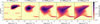 |
Fig. 1. Stacked temperature-density diagrams for all gas cells around galaxy clusters and groups in IllustrisTNG, considering different radial apertures from cluster central regions R[R200]< 1 up to 4 < R[R200]< 5. |
Moreover, according to Artale et al. (2022), who probed the large-scale distribution of ionised metals in IllustrisTNG, we can relate the gas density-temperature diagrams in Fig. 1 to their metal abundance, depending on the cluster-centric distance, and compare them with UV and optical wavelength observations. Recently, Artale et al. (2022) found that Mg II, C II, and Si IV are efficient tracers of the halo gas in dense environment, whereas Ne VIII, N V, O VI, and C IV are better tracers of warm hot and low-density gas (WHIM) inside filamentary structure at large scales (and z = 0). In particular, the small fraction of halo gas phase inside clusters (with T < 105 K and nH > 10−4 cm−3) is supposed to be condensed gas inside halos in high-density and low-temperature star-forming regions, as recently observed via Mg II absorption lines by Lee et al. (2021), Anand et al. (2022), and Mishra & Muzahid (2022). For example, Lee et al. (2021) showed that Mg II absorbers are more abundant inside clusters than outside them (> 2 R200).
We now probe the detailed radial profile of the different gas phases as a function of cluster-centric distance. Similarly to Galárraga-Espinosa et al. (2021), we define the mass fraction of a given gas phase as
with r being the 3D radial distance to the cluster centre,  the radial density of the ith gas phase, and
  the radial density of the total gas. The radial density of gas is computed by summing the mass of gas cells contained in spherical shells from a radius rk − 1 to rk, following Eq. (7):
with Nk being the number of gas cells and j contained in a spherical shell with a radius from rk − 1 to rk centred on the halo.
Following Eqs. (7) and (8), we computed the mass fraction of the five gas phases around each halo of our cluster sample. The mean radial profile of gas phases is presented in Fig. 2 by averaging over our halo sample, only considering galaxy clusters (M200 > 1014 M⊙ h−1) and only considering galaxy groups (M200 = [5−10] × 1013 M⊙ h−1), respectively, in the top, middle, and bottom panels. Figure 2 shows that the hot-gas phase is strongly dominating the interior of all halos (top panel). As expected, the gas must be strongly heated inside the deep gravitational potential wells of clusters, and thus it appears in the form of a hot plasma. Beyond the cluster region, the fraction of hot gas decreases, such that the gas becomes warmer and less dense (WHIM gas phase). The warm diffuse gas starts to dominate at distances larger than ∼0.9 R200 on average. However, we can see that the transition radius from hot to WHIM gas phase strongly differs for galaxy clusters and galaxy groups (middle and bottom panels). To illustrate this, we highlight the radius for which the hot-gas phase is no longer dominant in grey vertical lines in Fig. 2. The hot plasma extends up to 1.2 R200 inside galaxy clusters, whereas it is only dominant up to ∼0.6 R200 for galaxy groups. In addition, the hot gas mass fraction inside 1 R200 is about 93% for galaxy clusters, whereas it is only 68% for the galaxy groups. While hot plasma is largely extended and represents almost all of the gas inside galaxy clusters; gas in galaxy groups is a mixture of hot and warm dense gas.
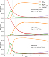 |
Fig. 2. Mean gas mass fraction profiles (see Eq. (7)) of the five different gas phases around all halos in our sample (top), only galaxy clusters (middle), and only galaxy groups (bottom). The radial boundary at which the hot gas phase is no longer dominant is shown by grey vertical lines and is about RHOT ∼ 0.91, 1.20 and 0.61 for the all groups and clusters, only clusters, and only groups, respectively. |
The bottom panel of Fig. 2 shows that the transition from the hot to WHIM gas phase is different in galaxy groups because it implies a third gas phase, the warm circum-galactic medium (WCGM), which has a similar temperature to the WHIM but is denser (see Fig. 1). The shallower gravitational potential of galaxy groups is not deep enough to heat the gas up to 107 K beyond the core region (> 0.6 × R200). At a greater distance, the gas temperature decreases first, with the gas transiting to the warm dense phase (WCGM), and then density decreases at 0.8 R200, transforming the gas in a diffuse and warm phase (WHIM). According to Martizzi et al. (2019), a WCGM gas phase must be created by shock heating and feedback of massive galaxies, and is located mostly in the vicinity of massive galaxies and inside galaxy groups. We confirm here that the WCGM phase is one of the dominant phases inside galaxy groups accounting for 23% of the mass within R < R200, with a peak contribution at around 0.7 R200.
Outside groups and clusters, typically beyond a distance of ≳1 R200, the WHIM gas phase largely dominates and tends to smoothly peak at around 2 R200. These radial distances are typically the infalling regions around clusters where gas is expected to be located inside the cosmic filamentary pattern connected to clusters (see e.g. Eckert et al. 2015, for observational evidence). In this region, the fraction of hot gas remains non-negligible, with about 13% of the total mass of gas from 1 to 3 R200. In fact, this small fraction of hot gas is expected to be in the form of small massive clumps located in cosmic filaments (Zhuravleva et al. 2013; Angelinelli et al. 2021). Far from the group and cluster centres (> 3 R200), the warm diffuse gas remains the dominated phase. Indeed, WHIM gas is supposed to be the dominant phase in the Universe with a mass fraction of around 46% according to Martizzi et al. (2019). We note that in our case, at distances of 5 × R200, the mass fraction of WHIM is quite high, with a value of 70%. This is consistent with the findings of Galárraga-Espinosa et al. (2021), who show that a WHIM gas phase slowly decreases up to 20 Mpc away from the spine of denser filaments. We can thus expect similar behaviour for a radial WHIM fraction profile around clusters.
We finally notice that, far from cluster centres at around 2.5 R200, the WHIM gas phase starts to decrease in favour of diffuse IGM. It is related to the presence of cold diffuse gas in galaxies. The increase of diffuse IGM at around 2 R200 from cluster centres is in agreement with results from Mostoghiu et al. (2021), who show that cold gas in infalling galaxies is completely depleted at 1.7 R200 from cluster centres (see also Arthur et al. 2019; Singh et al. 2020; Zhu et al. 2021a; Song et al. 2021, on the impact of filaments and cluster environments on the depletion of cold gas in infalling galaxies).
3.2. The gas dynamics
Beyond the temperature-density gas phases, it is also of prime importance to probe gas motions in order to investigate their infall from large-scale environments to clusters. The dynamics of the gas is explored in phase-space coordinates (velocity, position) following the definitions presented by Oman et al. (2013). Considering the 3D vector position, r, and 3D vector velocity, v, of each gas cell, we can identify all gas cells by their 6D coordinates (rx, ry, rz, vx, vy, vz). At the same time, each cluster is characterised by its central position, rc, and its 3D velocity, vc (the halo velocity is computed as the sum of the mass-weighted velocities of all particles/cells in the halo, pre-computed by the IllustrisTNG collaboration). Considering these phase-space coordinates, we can define the radial velocity of each gas cell relatively to their associated host cluster environment, such as:

Note that the sign of v3D allows us to distinguish between the infalling gas (v3D < 0) and the outgoing gas (v3D > 0) around a given cluster. In order to stack gas radial velocities for all cluster environments, we normalise them by the overall velocity dispersion σ3D, which is the root-mean-square of the radial gas velocity v3D within R200 of each cluster.
The velocity-position diagram is commonly used to probe the infall of galaxies into clusters (Dacunha et al. 2022). We can typically consider three different dynamical regimes in the velocity-position diagram: (i) infalling material with v3D < 0 and R > R200, (ii) backsplash material with v3D > 0 and R > R200, and (iii) virialised material inside clusters with R < R200 characterised by shell crossing caustics in velocity-position diagrams. In this frame, galaxies start their infall far from the cluster centre and increase their velocity as they approach the cluster. When they are close to the cluster, they first infall and then move away from the cluster (to form the backsplash population), and then they transit between infall and backsplash, until they are captured by the gravitational potential wells of the cluster, forming the virialised population (R < R200) (see Fig. 2 of Arthur et al. 2019, for a schematic view of the phase-space plane).
In Fig. 3, we present a phase-space diagram for gas in cluster environments. They are obtained by stacking all gas cells (left panels), only hot gas (middle panels), and only WHIM gas (in right panels) for the 415 halos of our sample (top panels), only the 149 galaxy clusters with M200 > 1014 M⊙ h−1 (middle panels), and only the galaxy groups with M200 = [5−10] × 1013 M⊙ h−1 (bottom panels). In the top left panel, the stacked phase-space diagram of all gas cells in all cluster environments shows the three dynamical regimes: virialised gas inside clusters, infalling gas with high infalling velocity, and a splashback gas component with positive velocity outside clusters (identically to Mostoghiu et al. 2019; Dacunha et al. 2022 for galaxy distribution). In more detail, we see that the virialised gas inside clusters (R < R200) is the hot-gas phase, as shown in the top middle panel. This hot plasma is virialised, i.e. there is an equal balance between inflow and outflow motions with low velocity values of −2.5σ < vWHIM < 2.5σ. Focusing on the WHIM gas phase in the top right panel, we can distinguish two distinct dynamical behaviours. At cluster peripheries, from ∼1 to ∼2 R200, the WHIM gas is a combination of slowly infalling and backsplash gas (−2σ < vWHIM < 2σ). In contrast to hot gas, the WHIM inflow and outflow motions are not balanced, and infalling gas is significantly dominant. This means that this WHIM gas is accumulating at cluster peripheries by slowly infalling inside clusters and with a minor fraction that is ejected outside clusters. Beyond the cluster peripheries, at distances from 1.5 to 5 R200, the WHIM gas is also rapidly infalling on clusters with high velocity values, typically −5σ < vWHIM < −2σ < v3D. According to Rost et al. (2021), gas is entering clusters with turbulent motions. This might explain why the WHIM gas phase is accumulated and ejected at cluster peripheries (∼1 R200). Moreover, Rost et al. (2021) also show that gas is preferentially infalling from filaments. Therefore, one can suppose that fast infalling WHIM (R > R200 and vWHIM < −2σ) must be inside cosmic filaments, whereas the WHIM backsplash material (∼R200 and vWHIM > 0) should leave the cluster centre outside filaments.
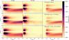 |
Fig. 3. Stacked phase-space diagrams for all gas cells (left panels), only hot gas (middle panels), and warm-hot intergalactic medium (right panels). All groups and clusters are considered in top panels, only galaxy clusters (with M200 > 1014 M⊙ h−1) in the middle panels, and only galaxy groups (with M200 = [5−10] × 1013 M⊙ h−1) in the bottom panels. |
Regarding the halo mass dependency, we can compare middle and bottom panels showing clusters and groups of galaxies, respectively. Focusing on all gas cells, there are no significant differences between clusters and groups. However, considering hot and WHIM gas phases separately, we can see that galaxy groups and clusters show different dynamical behaviour. The hot gas is more spatially extended inside galaxy clusters compared to groups, as already found in the radial gas phase profile (Fig. 2). Also, we can notice that only galaxy clusters present residual hot-gas distribution beyond R200. This small fraction of infalling hot gas must be associated with dense clumps of matter inside cosmic filaments, as proposed by Angelinelli et al. (2021). Regarding the WHIM velocity-position diagram, we can see that the warm gas dynamics is different for groups and clusters. While the WHIM gas phase is mostly in the form of fast infalling gas (high velocity and low velocity dispersion) outside galaxy clusters, WHIM gas around groups is strongly accumulating at their outskirts (with a large scatter in velocity and a backsplashing motion from 1 to 2 R200). This suggests that the WHIM gas phase is mostly inside filaments at cluster peripheries, whereas WHIM gas around groups is infalling and ejected at cluster peripheries.
We conclude that the hot gas is the dominant phase inside cluster halos (R < R200), mostly governed by the low velocity dispersion of well-balanced inflow and outflow motions (|vWHIM|≲2.5σ). In contrast, outside of groups and clusters (R > R200), the gas is mainly in the form of warm diffuse gas. The WHIM gas phase outside halos can be separated into two distinct dynamical regimes: accumulating gas slowly infalling from ∼1 to ∼2 R200 and fast infalling gas at distances over 1.5 R200. Cluster peripheries are thus crucial places to probe the transition between hot and warm gas and to probe the complex dynamics of infalling WHIM gas. In fact, it is in these regions that the gas is expected to flow from filaments into clusters, with turbulent motions (Rost et al. 2021; Vallés-Pérez et al. 2021), and where accretion shocks might arise (Shi et al. 2020; Zhang et al. 2020, 2021a; Zhu et al. 2021b). Following these findings on the radial gas properties, we focused the rest of our exploration of the azimuthal gas distribution on the cluster environment, concentrating on two main gas phases in two different radial apertures: the hot medium up to 1 R200 and the WHIM from 1 to 2 R200.
4. Azimuthal distribution as a proxy of structural properties of clusters
In this section, we define the aperture multipole formalism and use this technique on gas azimuthal distribution to statistically highlight angular-dependent features in comparison to the ‘reference’ DM distribution. This technique focuses on 2D spatial distribution and has already been applied to weak lensing maps (Dietrich et al. 2005) and projected photometric galaxy distribution (Gouin et al. 2020). In this study, the azimuthal symmetries of gas and DM were explored as a function of cluster structural properties (defined in Sect. 2) to probe if they are good tracers of the structural features of cluster halos.
In this section and the next one, a general colour and style code is used in the plots: (i) hot gas, WHIM, and dark matter are, respectively, in red, orange, and blue or black; (ii) the mean profiles are shown by solid lines, and the error bars are the mean errors computed by bootstrap re-sampling; (iii) the number of objects used to compute the average in each bin (of the x-axis) is written above the figures in grey; (iv) the Spearman rank correlation coefficient ρSP(X, βm) is written on the figure, with X being the cluster property and βm the multipolar ratio at the multipole order, m, as defined below. The p value of the correlation coefficient remains lower than 10−3 for each plot.
4.1. Formalism of multipole moments, Qm
The aperture multipole moments of 2D density fields were first introduced by Schneider & Bartelmann (1997) for weak lensing map application. It consists of a multipole decomposition of a surface density in harmonics modes, m, integrated over a given radial aperture, such as
where Σ(R, ϕ) is the 2D matter distribution in polar coordinates centred on the cluster centre. The 2D radial aperture ΔR = (Rmax, Rmin) is also centred on the cluster centre with Rmin and Rmax the radii delimitating the circular shell. For illustration, we show the different azimuthal symmetries quantified by the multipole moments, Qm, in Fig. 4, with monopole (m = 0), dipole (m = 1), quadrupole (m = 2), and so on. Using the multipolar expansion of 2D matter distribution around galaxy clusters, this technique succeeded in highlighting both the elliptical shape of clusters (see e.g. Clampitt & Jain 2016; Shin et al. 2018), and filamentary patterns at cluster outskirts (Dietrich et al. 2005; Mead et al. 2010; Gouin et al. 2017; Codis et al. 2017) from a 2D-projected DM distribution.
 |
Fig. 4. Illustration of different azimuthal symmetries as a function of harmonic orders, m. |
In order to assess the relative weight of one azimuthal symmetry traced by the order m relatively to the circular one, we define the multipolar ratio βm as

with |Qm| being the modulus of the aperture multipole moment at the order m. By decomposing surface mass density in harmonic expansion terms, Schneider & Weiss (1991) showed that  for a matter distribution Σ(θ)∝cos(2θm). Therefore, the value of the multipolar ratio βm varies between 0 and 1/2, such that βm = 0 for a circular matter distribution and βm = 1/2 for a matter distribution describing the azimuthal symmetry at the order m (see also Vallés-Pérez et al. 2020, for a similar definition).
We aim to probe different aspherical features from the dipolar signature traced by m = 1, to large harmonic orders (small angular scale patterns) up to m = 9. Indeed, Gouin et al. (2020) showed that azimuthal matter distribution away from the cluster centres can be described by the sum of multipolar moments from m = 1 to m ∼ 9, tracing multi-angular scale filamentary patterns. In Fig. A.1, we present the evolution of the different multipolar ratio, βm, as a function of radial distance for m = 1 to 9. As expected, the multipolar ratio increases with the radial distance, similarly to the more commonly used azimuthal scatter technique (Eckert et al. 2015). Indeed, anisotropy of matter distribution is expected to increase with the radial distance from the halo centre, as also detailed in Despali et al. (2017) for the ellipticity term.
From Eqs. (10) and (11), we computed the multipolar ratio βm for m from 1 to 9, in both (hot and WHIM) gas and DM distribution for each cluster. We projected the matter distribution enclosed inside a sphere of radius R3D = 5 R200 centred on each cluster considering the three different projection axes (along x-, y- and z- axis) of the simulation box. Therefore, the cluster sample increases from 415 clusters to 1245 2D-projected maps of cluster mass distribution. In Fig. 5, we show an example of the DM, the hot medium, and the WHIM 2D-projected distribution around a simulated cluster. As discussed in Sect. 3, the hot gas is mostly located inside the cluster halo (typically < R200), whereas WHIM traces the infalling gas outside the cluster. In the following, we thus focus on the hot medium to explore the gas inside clusters, and the WHIM to probe the gas filamentary pattern outside clusters.
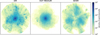 |
Fig. 5. Illustration of dark matter (left), hot gas (middle), and WHIM (right) 2D projected distribution up to 5 R200 of one simulated galaxy cluster. The cyan ellipse on dark matter traces the ellipticity of the DM halo ( |

4.2. Impact of cluster structural properties
We now explore the azimuthal symmetries traced by hot gas and DM distribution inside clusters and see if they are related to the structural properties of cluster halos. To do so, we focus on different angular properties of matter distribution by considering the multipolar ratio, βm, at a different multipolar order, m. Following the description in Sect. 2, the structural properties we considered are the halo ellipticity, ϵ, the centre offset, Roff, and the mass fraction of substructures, fsub.
In Fig. 6, we show the multipolar ratio, βm, and its mean, considering different radial apertures R, and as a function the structural properties of cluster halo. The multipolar moments and their ratios have been computed for both DM (at different radial apertures) and hot gas (with radial aperture R < R200); these are shown in blue and red, respectively.
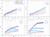 |
Fig. 6. Distribution of βm parameter as a function of structural halo properties. Top left panel: distribution of βm dipole contribution (m = 1) as a function of the centre-of-mass offset. Top right panel: distribution of βm quadrupole contribution (m = 2) as a function of the 2D ellipticity of DM. Bottom left panel: distribution of βm quadrupole contribution (m = 2) as a function of the 3D ellipticity of DM. Bottom right panel: high azimuthal symmetries’ βm contribution (summing contributions from m = 3, 4, 5, 6, 7, 8, 9) as a function of the mass fraction of sub-structures. The mean profiles of β are shown by solid lines, and the error bars are the mean errors computed by bootstrap re-sampling. The β values for the DM distribution with apertures R < 0.5 × R200, R < 1 × R200 and R < 2 × R200, are, respectively, plotted in light, medium, and dark blue. The β values for 2D hot-gas distribution with R < R200 are plotted in red. In each panel, the number of objects used to compute the average in each x-axis bin (shown in grey dotted lines) is written above the figures in grey. |
In the top left panel, we show the possible correlation between the centre offset and the dipolar symmetry traced by β1. We focus on m = 1, because the dipolar symmetric excess must in principle reflect the mis-centring of mass distribution, whereas the offset centre parameter directly quantifies differences between the peak centre and centre of mass. We find that the dipolar symmetries of DM and hot gas trace the centre offset of clusters well, with a correlation coefficient between β1 and Roff larger than ρSP > 0.5. We note that, as expected when taking into account larger mass distribution up to 2 R200, we increase the correlation between dipolar ratio, β1, and centre offset.
The top right panel shows the level of quadrupolar symmetry (with m = 2) as a function of the 2D ellipticity of DM halos. In agreement with previous studies (Clampitt & Jain 2016; Shin et al. 2018), we confirm that the quadrupolar decomposition of the DM density field is strongly correlated with the elliptical shapes of the halo with ρSP ∼ 0.8. We note that increasing the radial aperture above R200 does not significantly increase the correlation coefficient, suggesting that the halo shape information is mostly contained inside R200. We also found a good correlation between the quadrupolar symmetry of hot gas and the DM ellipsoidal shape. In fact, Okabe et al. (2018) showed that the gas distribution follows the elliptical shape of DM but tends to be more circular due to the dissipative baryonic processes (see also Velliscig et al. 2015). In the present study, we find that the hot gas quadrupolar signature is smaller than the DM ( ), confirming that the hot gas distribution tends to be more circular than the DM one. This is also illustrated in Fig. B.1 and confirms relations between both hot gas and DM ellipticity and their quadrupoles.
In the bottom left panel of Fig. 6, we extend our investigation to the 3D elliptical halo shape. As expected, the correlation between ellipticity and quadrupole remains strong, even if high 3D ellipticity (ϵ3D > 0.15) is degenerate with the 2D quadrupolar ratio. Due to projection effects, a strongly elliptical halo shape can produce a low quadrupolar signature. This degeneracy is reduced by considering larger radial apertures, such that for a radial aperture of 2 R200, the quadrupolar ratio and 3D ellipticity are strongly correlated with a Spearman coefficient: ρSP ∼ 0.5.
In the bottom right panel of Fig. 6, we finally probe the amount of mass inside sub-halos via the fraction of sub-structures. To quantify this last structural property, the best choice is to consider larger harmonic orders, meaning small angular-scale decomposition. We directly sum multipolar ratios βm from m = 3 to 9 to obtain the overall level of azimuthal symmetries for small angular scales and compare it to the fraction of substructures. Multipolar ratio and fsub tend to correlate well for both hot gas and DM with correlation coefficients around ρSP ∼ 0.4. In particular, we can distinguish between low (fsub < 0.1) and high sub-structure fractions (fsub > 0.1), which is an important criterion to separate dynamically relaxed and non-relaxed clusters as proposed by Cui et al. (2017). As for 3D ellipticity, by considering large radial apertures (R < 2 R200) we significantly increase the correlation between the fraction of sub-structures and the level of azimuthal symmetries up to ρSP ∼ 0.6.
As illustrated in Fig. 4, the multipole moment at each order, m, represents different azimuthal symmetries. By probing the multipolar ratio, βm (defined in Eq. (11)), we computed the excess of one azimuthal symmetry at the order, m, relative to the circular symmetry (m = 0). At each harmonic order, m, the multipolar ratio highlights a different angular feature. They are by nature powerful tracers of distinct structural properties of cluster halos (as shown in Fig. 6). Considering m = 1, the monopolar ratio reflects the mis-centring of cluster mass distribution, whereas for m = 2 the quadrupolar excess correlates with the elliptical shape of clusters (as also discussed in Gouin et al. 2017, 2020). Moreover, as we increase the multipole order, m, the physical size of the angular pattern decreases, and thus we characterise small-scale structures. This explains why multipole modes from m = 3 to 9 are a good probe of the sub-structure fraction.
Even when considering 2D matter distribution, the correlation with its 3D structural properties is strong and can be further improved by integrating matter distribution beyond R200. Moreover, the azimuthal hot plasma distribution appears to follow the azimuthal DM distribution well, as shown via its significant correlation with the halo properties. The hot-gas plasma distribution remains smoother and more circular than DM, with lower values of the multipolar ratio, βm, for almost all orders, m.
5. Azimuthal distribution related to cluster physical properties
In this section, we do not attempt to distinguish between the different angular features in the 2D mass distribution, but we assess whether the overall departure from circular symmetry can be related to cluster physical properties. We thus focus on a single variable, β, to estimate the amount of azimuthal symmetries in excess compared to the circular one:

This azimuthal symmetric excess, β, is defined as the sum of all the azimuthal symmetry contributions up to the order N. As discussed in Appendix A, we chose N = 4 because adding larger orders (from 5 to 9) does not alter the conclusions of this section. Indeed, each multipole order from m = 5 to 9 contributes less than 10% to the matter multipolar expansion, and thus they constitute minor harmonic orders to represent matter distribution (as shown in Fig. A.1).
Based on the analysis of the radial gas distribution discussed in Sect. 3, we focus on two radial apertures and two gas phases. First, we consider the interior of clusters (R < R200) and we investigate the azimuthal symmetric excess β of both hot plasma and DM distributions. Secondly, we consider the cluster peripheries (1 < R[R200]< 2) and investigate the filamentary patterns in the WHIM and DM azimuthal distributions via the β variable. We also studied the azimuthal matter distribution for larger radial apertures from 2 to 5 R200. We found a weak correlation between the cluster physical properties and the azimuthal gas distribution for apertures 2 < R[R200]< 3, and the two quantities become uncorrelated beyond radial distances of 3 R200.
5.1. Mass and connectivity dependency
We first discuss the relation between departures from circular symmetry and the cluster mass inside (R < R200) and at the cluster outskirts (1 < R[R200]< 2), as shown in the top and bottom panels of Fig. 7, respectively. Focusing on the dark matter distribution inside halos (R < R200), we note that the azimuthal symmetric excess slowly increases with the cluster mass, on average. In fact, the non-circularity quantified by β is strongly dominated by the quadrupole (m = 2) inside clusters, and it traces the elliptical halo shape, as discussed in Sect. 4 and illustrated in Appendix B. Therefore, the increase of the azimuthal symmetric excess with the halo mass must reflect the increase of the DM halo ellipticity, in agreement with Despali et al. (2014). Nevertheless, we found that the correlation between the DM azimuthal symmetric excess and halo mass is low, with ρSP ∼ 0.1.
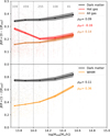 |
Fig. 7. Distribution of azimuthal symmetric excess β (as defined in Eq. (12)) as a function of the halo mass, inside clusters (R < R200) in the top panel and at cluster peripheries in (1 < R[R200]< 2) in the bottom panel. The mean profiles of β and their errors are shown in solid lines. The colours of points and lines represent different matter components: dark matter (black), hot gas (red), WHIM (orange), and all gas (light brown). In each panel, the number of objects used to compute the average in each bin of the x-axis (shown as grey dotted lines) is written above the figures in grey. |
Focusing on the hot gas inside clusters, we found that the anisotropy of hot gas distribution tends to decrease with the halo mass. Hot gas in galaxy groups (M200 < 1014 M⊙ h−1) appears more asymmetric than in massive clusters, on average. This might be explained by the fact that, as detailed in Sect. 3, hot gas is not the dominant component in groups (representing only 68% of all gas) and is concentrated in the core of galaxy groups (hot gas is only dominant up to R ∼ 0.6). In contrast, the ICM of massive clusters is almost exclusively in the form of hot plasma and spatially extends up to R ∼ 1.2. One can thus interpret that behaviour by the fact that hot gas material inside massive clusters is mostly gravitationally heated, whereas in galaxy groups the hot gas distribution might be governed by anisotropic accretion processes, and thus it appears highly asymmetric. In agreement with this interpretation, we found that considering all gas cells inside group and cluster halos, the anti-correlation between azimuthal symmetry of gas component and halo mass is removed. It means that only the hot plasma medium is strongly anisotropic inside galaxy groups.
Focusing on cluster peripheries from 1 to 2 R200 in the bottom panel of Fig. 7, we show that the anisotropic signatures of DM and WHIM are increasing with the cluster mass. The small increase of DM azimuthal symmetric excess with halo mass must be induced by the amount of filamentary structures that are expected to be more massive and more numerous around massive objects compared to low-mass ones (Aragón-Calvo et al. 2010b; Codis et al. 2018; Sarron et al. 2019; Kraljic et al. 2020; Gouin et al. 2021). Regarding the azimuthal level of WHIM gas, there is a strong mass dependency: WHIM distribution around massive clusters is significantly more asymmetric than around low-mass groups. In fact, we see in Fig. 3 that WHIM gas from 1 to 2 R200 is rapidly infalling into massive clusters, whereas WHIM in galaxy group environments is slowly infalling and back-splashing. In agreement with this dynamical picture, one can expect that WHIM gas is strongly asymmetric around massive objects because it is infalling along filamentary structures. This is consistent with Rost et al. (2021), who found that gas preferentially enters into massive clusters funneled by filaments. In contrast, WHIM around groups is more isotropically distributed because it is accumulating (and ejected) at the group peripheries, and thus it must trace filaments more faintly.
To confirm if WHIM anisotropic distribution outside clusters is, in general, the result of filamentary pattern surrounding them, in Fig. 8 we show the azimuthal symmetric excess, β, as a function of the connectivity of halos. As we can see, the number of cosmic filaments that are connected to clusters and the departure from spherical symmetry are significantly correlated for both the DM and the WHIM gas phase. In agreement with Galárraga-Espinosa et al. (2021), who found that WHIM gas phase is strongly dominant in cosmic filaments, we conclude that the azimuthal distribution of WHIM tends to follow DM by tracing cosmic filamentary structures connected to clusters at their peripheries.
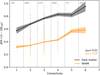 |
Fig. 8. Distribution of azimuthal symmetric excess β (as defined in Eq. (12)) computed at cluster peripheries in (1 < R[R200]< 2) as a function of the halo connectivity, for DM (black) and WHIM (orange). The mean profiles of β and their errors are shown as solid lines. The number of objects used to compute the average in each bin of the x-axis (shown with grey dotted lines) is written above the figures in grey. |
5.2. Accretion history dependency
We see that the hot plasma traces the halo properties of clusters well, whereas the WHIM azimuthal distribution correlates with filamentary patterns connected to clusters. Given these findings, one can ask oneself whether the gas azimuthal distribution can also trace the overall cluster dynamics and its recent mass-assembly history, as well as DM. We refer the reader to Sect. 2 for details on the definitions of the mass-accretion rate Γ (see Eq. (1)) and the formation redshift zform (see Eq. (2)), which are two proxies of cluster mass-assembly history, and the relaxedness parameter χDS used to estimate the cluster dynamical state (see Eq. (6)).
In Fig. 9, we show the dependency of azimuthal symmetric excess, β, with the different cluster properties: relaxedness (left panels), mass-accretion rate (middle panels), and formation redshift (right panels). The azimuthal symmetric excess of hot gas and DM inside clusters (R < R200) is presented in the top panels, whereas the bottom ones show the WHIM and DM anisotropic level at cluster peripheries (1 < R[R200]< 2).
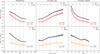 |
Fig. 9. Distribution of azimuthal symmetric excess, β (as defined in Eq. (12)), computed inside clusters (R < R200) in top panels and at cluster peripheries (1 < R[R200]< 2) in bottom panels, as a function of different halo properties: level of relaxation on the left, mass-accretion rate in the middle, and formation redshift on the right. The mean profiles of β and their errors are shown in solid lines. The number of objects used to compute the average in each bin of the x-axis (shown with grey dotted lines) is written above the figures in grey. |
The departure from circular symmetry is first analysed as a function of the relaxation level of clusters (left panels). We found that the more circular the matter distribution (β → 0), the more dynamically relaxed the cluster halo (χDS > 1). Inside clusters, halo relaxedness and asymmetry are strongly correlated for both DM and hot gas, with ρSP ∼ 0.5, showing that the azimuthal distribution of hot plasma is a powerful probe of cluster dynamics. This result is in agreement with previous investigations on ICM asymmetry to probe the cluster dynamical state (Vazza et al. 2011; Eckert et al. 2012; Capalbo et al. 2021). Moreover, at cluster peripheries the azimuthal distribution of WHIM and DM also traces the cluster relaxation level well. This can be explained by the fact that the cluster dynamical state must be affected by the number of cosmic filaments connected to clusters, as shown in Gouin et al. (2021).
Secondly, the influence of the cluster’s mass-assembly history on the azimuthal matter distribution is investigated by considering two variables: the mass-accretion rate and the formation redshift of clusters in the middle and right panels, respectively. Both cluster accretion history proxies are correlated with gas and DM azimuthal symmetry excess, in particular inside cluster halos, with ρSP ∼ 0.6. The faster the cluster accretes material and the more recently formed, the more asymmetric its hot medium distribution. This is coherent with the result of Chen et al. (2020), who show that the ellipticity of the ICM seems to be an imprint of the mass-assembly history of clusters. Besides the ICM, we found that WHIM and DM inside the filamentary structure at the cluster periphery show a similar trend. Indeed, Gouin et al. (2021) show that the cosmic filaments connected to clusters affect cluster assembly history. Nevertheless, the correlation between the azimuthal symmetry and mass-assembly history decreases up to ρSP ∼ 0.3 at cluster peripheries, suggesting that the mass distribution in the inner regions is more sensitive to the cluster past accretion history.
6. Discussion
In this study, we applied the azimuthal decomposition technique to the spatial distribution of a simulated group and cluster gas phases defined using temperature-density-selected gas cells projected in 2D. We show that the 2D azimuthal gas distribution is related to the 3D cluster mass distribution from their shape to their connected filaments. The correlation between azimuthal symmetric excess (in 2D) and the connectivity of clusters shows that considering only the main contribution of harmonic decomposition successfully traces the filamentary patterns (see also Vallés-Pérez et al. 2020). However, we can expect that the 3D spherical harmonics must be more correlated with 3D ellipticity and 3D connectivity than 2D harmonics one, due to the small corrections provided by the full spherical harmonic decomposition.
The next step in the use of the multipolar analysis will be to apply 2D multipole moment formalism to 2D mock X-ray and SZ images to accurately evaluate the efficiency of such a technique on future data by taking into account observational effects such as finite angular resolution due to instrumental beam, noise, and so on (see e.g. Green et al. 2019; De Luca et al. 2021; Comparat et al. 2020; Gianfagna et al. 2021 for mock X-ray images of clusters). This approach could be a powerful tool to highlight patterns in current and upcoming observations of the cosmic gas at the peripheries of galaxy clusters, such as those of X-COP (Tchernin et al. 2016), Cluster Heritage (CHEX-MATE Collaboration 2021), and eROSITA (Predehl et al. 2021; Comparat et al. 2022). Indeed, the eROSITA mission is expected to provide the necessary resolution to statistically probe connected gas filaments around clusters with the harmonic decomposition technique, as it has already allowed the discovery of a long WHIM filament (Reiprich et al. 2021; Veronica et al. 2022; Brüggen et al. 2021; Biffi et al. 2022). Moreover, on a much smaller scale than the galaxy clusters (at a few kpc), the multipole decomposition might also be a powerful tool for other applications, such as quantifying the anisotropic distribution of a circumgalactic medium around black holes, as predicted by Truong et al. (2021), to constrain supermassive black hole feedback from X-ray observations.
7. Conclusions
In this study, we explored how gas and DM components are distributed in galaxy cluster environments from their cores to their connection to cosmic filaments. We focused on the matter distribution in 415 galaxy cluster environments, defined as the regions extending up to 5 R200, extracted from the IllustrisTNG simulation. Their gas phases, defined thanks to the temperature-density diagram, and their motions were first investigated as a function of the cluster-centric distance and mass. This allowed us to identify the most relevant gas phases and radial apertures to further study the azimuthal distribution of the gas in clusters. By decomposing the matter distribution in harmonic space, we statistically explored the angular features, also called azimuthal symmetries, in gas and DM distributions around clusters. Previous multipolar expansion of dark matter (Gouin et al. 2017) and galaxy (Gouin et al. 2020) distributions in cluster environments have revealed the usefulness of this approach to statistically probe the cosmic filamentary pattern outside clusters. In the present extension to the studies by Gouin et al. (2017, 2020), we focused on gas distribution to explore how azimuthal symmetries of gas in different phases trace cluster physical and dynamical properties as well as the ‘reference’ dark matter distribution. The radial and azimuthal gas distribution from cluster inner regions to their connection to filaments lead us to the conclusions described as follows.
-
(1)
Galaxy cluster environments are key regions where the warm diffuse gas is infalling into clusters and heated to become the hot plasma inside cluster cores (as also discussed by Martizzi et al. 2019; in the large cosmic-web picture). In detail, the hot-gas phase is dominant inside clusters, up to around 1 R200, and it is well virialised with an equal balance between slow inflow and outflow motions. In contrast, the gas outside clusters (R > R200) is mainly in the form of WHIM and presents two distinct dynamical regimes: the accumulating gas at cluster peripheries from ∼1 to ∼2 R200 with both slowly ejected and infalling gas motions, and the rapidly infalling gas at a distance from the centre of R > 1.5 R200. These findings can be likened to those of Rost et al. (2021), who found that cosmic gas is fast infalling into clusters along filaments and leaves the cluster outside filaments.
-
(2)
Groups and clusters show different radial transitions from hot-to-warm gas phases. While galaxy clusters present an extended core of hot plasma up to 1.2 R200, the galaxy groups contain different gas phases with a core of hot plasma (up to 0.6 R200), a shell of warm dense gas (WCGM phase), and diffuse warm gas (WHIM phase) beyond R > 0.8 R200. Groups and clusters also show different WHIM motions at their outskirts. While the WHIM gas phase is mostly rapidly infalling outside clusters, it is accumulating and slowly infalling at the peripheries of groups.
-
(3)
The azimuthal symmetric features of gas and DM distributions are strongly correlated with distinct structural properties of the cluster halos. In particular, the dipolar symmetry reflects the halo centre offset, the quadrupolar symmetry describes the halo ellipticity, and larger harmonic decomposition orders trace the amount of halo sub-structures. The azimuthal hot plasma distribution appears to follow the DM one well, tracing the structure of the cluster halo, even if the hot gas tends to be smoother and more circular than the DM distribution (as expected from the ellipsoidal shape of DM and hot gas found by Okabe et al. 2018).
-
(4)
Focusing on mass dependency, we found that the hot gas is more asymmetric inside galaxy groups than in clusters. We relate this to the fact that the hot gas does not represent the overall gas distribution inside groups, but is rather concentrated in group cores and must be subject to distortion by anisotropic accretion processes. In contrast, the ICM of massive clusters is almost exclusively composed of gravitationally heated gas inside R200 (at 93%), which can thus explain its more isotropic shape.
-
(5)
At cluster peripheries, the WHIM and DM azimuthal symmetries increase with cluster mass, in agreement with the expected increase of the cosmic filamentary signature with mass in harmonic space (Gouin et al. 2020). WHIM at peripheries of massive clusters better traces cosmic filament patterns than in the low-mass clusters and groups. This can be explained according to our dynamical analysis of WHIM gas and results from Rost et al. (2021) due to the fact that WHIM around groups is both slowly infalling in filaments and outflowing from groups out of filaments.
-
(6)
At cluster peripheries, the asymmetric signatures of WHIM and DM distributions increase significantly with the number of connected filaments, showing that the matter azimuthal symmetric excess in cluster infalling regions (from 1 to 2 R200) is an imprint of cluster filamentary patterns. Therefore, the WHIM gas phase, as it follows the DM distribution, appears to trace connections to the cosmic filaments well. We also confirm that gas in filaments outside clusters is mostly in the form of a WHIM phase, in agreement with Galárraga-Espinosa et al. (2021).
-
(7)
We found that the gas azimuthal distribution is affected by the past assembly history of clusters and that it is a good tracer of its current dynamical state, as good as the ‘reference’ DM distribution. In agreement with previous ICM investigations in simulations (see e.g. Vazza et al. 2011), we confirm that by using this azimuthal decomposition technique, departures from circular symmetry in hot-gas distribution are stronger for more dynamically unrelaxed, faster-accreting, and later formed clusters. Beyond these findings, we show that these relations between gas distribution and cluster properties can be extended to the warm diffuse gas phase located in cosmic filaments at cluster peripheries.
By probing both the radial and azimuthal gas distribution in galaxy cluster environments, we describe the radial transition from hot gas, dominant in the inner regions, to WHIM gas, dominant at the peripheries, during their infall along cosmic filaments. We found that gas properties and their distribution are strongly affected by cluster environments up to about 2 R200. Beyond a radial distance of 4 R200, the cluster environments no longer impact gas azimuthal distribution. Moreover, by using this novel reliable technique based on multipolar decomposition, we statistically probed azimuthal symmetric features in the gas distribution up to the connection with filaments at cluster peripheries. Our study constitutes a first attempt to statistically explore azimuthal gas distribution in 2D-projected gas maps in its main phases, comparably to gas observations in galaxy cluster environments (Eckert et al. 2015). In real data, this approach might require high angular resolution (similarly to Vallés-Pérez et al. 2021; Capalbo et al. 2021) and could be a powerful tool to highlight patterns in current and future observations of the cosmic gas at the peripheries of galaxy clusters (Tchernin et al. 2016; Barcons et al. 2017; XRISM Science Team 2020; CHEX-MATE Collaboration 2021; Simionescu et al. 2021).
Acknowledgments
We thank the anonymous referee for his/her report and helpful comments and suggestions. This research was supported by the funding for the ByoPiC project from the European Research Council (ERC) under the European Union’s Horizon 2020 research and innovation program grant agreement ERC-2015-AdG 695561 (ByoPiC, https://byopic.eu). The authors thank the very useful comments and discussions with all the members of the ByoPiC team. We thank the IllustrisTNG collaboration for providing free access to the data used in this work. C.G. is supported by a KIAS Individual Grant (PG085001) at Korea Institute for Advanced Study (KIAS). She is grateful to Professor Changbom Park for stimulating discussions.
References
- Akamatsu, H., Fujita, Y., Akahori, T., et al. 2017, A&A, 606, A1 [NASA ADS] [CrossRef] [EDP Sciences] [Google Scholar]
- Anand, A., Kauffmann, G., & Nelson, D. 2022, MNRAS, 513, 3210 [NASA ADS] [CrossRef] [Google Scholar]
- Angelinelli, M., Vazza, F., Giocoli, C., et al. 2020, MNRAS, 495, 864 [NASA ADS] [CrossRef] [Google Scholar]
- Angelinelli, M., Ettori, S., Vazza, F., & Jones, T. W. 2021, A&A, 653, A171 [NASA ADS] [CrossRef] [EDP Sciences] [Google Scholar]
- Ansarifard, S., Rasia, E., Biffi, V., et al. 2020, A&A, 634, A113 [NASA ADS] [CrossRef] [EDP Sciences] [Google Scholar]
- Aragón-Calvo, M. A., Platen, E., van de Weygaert, R., & Szalay, A. S. 2010a, ApJ, 723, 364 [Google Scholar]
- Aragón-Calvo, M. A., van de Weygaert, R., & Jones, B. J. T. 2010b, MNRAS, 408, 2163 [CrossRef] [Google Scholar]
- Artale, M. C., Haider, M., Montero-Dorta, A. D., et al. 2022, MNRAS, 510, 399 [Google Scholar]
- Arthur, J., Pearce, F. R., Gray, M. E., et al. 2019, MNRAS, 484, 3968 [Google Scholar]
- Barcons, X., Barret, D., Decourchelle, A., et al. 2017, Astron. Nachr., 338, 153 [NASA ADS] [CrossRef] [Google Scholar]
- Biffi, V., Dolag, K., Reiprich, T. H., et al. 2022, A&A, 661, A17 [Google Scholar]
- Bond, J. R., & Myers, S. T. 1996, ApJS, 103, 63 [NASA ADS] [CrossRef] [Google Scholar]
- Bonjean, V., Aghanim, N., Salomé, P., Douspis, M., & Beelen, A. 2018, A&A, 609, A49 [NASA ADS] [CrossRef] [EDP Sciences] [Google Scholar]
- Bonnaire, T., Aghanim, N., Decelle, A., & Douspis, M. 2020, A&A, 637, A18 [NASA ADS] [CrossRef] [EDP Sciences] [Google Scholar]
- Bonnaire, T., Decelle, A., & Aghanim, N. 2021, arXiv e-prints [arXiv:2106.09035] [Google Scholar]
- Brüggen, M., Reiprich, T. H., Bulbul, E., et al. 2021, A&A, 647, A3 [NASA ADS] [CrossRef] [EDP Sciences] [Google Scholar]
- Capalbo, V., De Petris, M., De Luca, F., et al. 2021, MNRAS, 503, 6155 [Google Scholar]
- Cautun, M., van de Weygaert, R., & Jones, B. J. T. 2013, MNRAS, 429, 1286 [NASA ADS] [CrossRef] [Google Scholar]
- Cautun, M., van de Weygaert, R., Jones, B. J. T., & Frenk, C. S. 2014, MNRAS, 441, 2923 [Google Scholar]
- Cen, R., & Ostriker, J. P. 1999, ApJ, 514, 1 [NASA ADS] [CrossRef] [Google Scholar]
- Cen, R., & Ostriker, J. P. 2006, ApJ, 650, 560 [Google Scholar]
- Chen, H., Avestruz, C., Kravtsov, A. V., Lau, E. T., & Nagai, D. 2019, MNRAS, 490, 2380 [NASA ADS] [CrossRef] [Google Scholar]
- Chen, Y., Mo, H. J., Li, C., et al. 2020, ApJ, 899, 81 [NASA ADS] [CrossRef] [Google Scholar]
- CHEX-MATE Collaboration (Arnaud, M., et al.) 2021, A&A, 650, A104 [NASA ADS] [CrossRef] [EDP Sciences] [Google Scholar]
- Christiansen, J. F., Davé, R., Sorini, D., & Anglés-Alcázar, D. 2020, MNRAS, 499, 2617 [NASA ADS] [CrossRef] [Google Scholar]
- Cialone, G., De Petris, M., Sembolini, F., et al. 2018, MNRAS, 477, 139 [Google Scholar]
- Clampitt, J., & Jain, B. 2016, MNRAS, 457, 4135 [Google Scholar]
- Codis, S., Pichon, C., & Pogosyan, D. 2015, MNRAS, 452, 3369 [Google Scholar]
- Codis, S., Gavazzi, R., Pichon, C., & Gouin, C. 2017, A&A, 605, A80 [NASA ADS] [CrossRef] [EDP Sciences] [Google Scholar]
- Codis, S., Pogosyan, D., & Pichon, C. 2018, MNRAS, 479, 973 [Google Scholar]
- Cole, S., & Lacey, C. 1996, MNRAS, 281, 716 [NASA ADS] [CrossRef] [Google Scholar]
- Comparat, J., Eckert, D., Finoguenov, A., et al. 2020, Open J. Astrophys., 3, 13 [Google Scholar]
- Comparat, J., Truong, N., Merloni, A., et al. 2022, A&A, submitted [arXiv:2201.05169] [Google Scholar]
- Cui, W., Power, C., Borgani, S., et al. 2017, MNRAS, 464, 2502 [NASA ADS] [CrossRef] [Google Scholar]
- Dacunha, T., Belyakov, M., Adhikari, S., et al. 2022, MNRAS, 512, 4378 [NASA ADS] [CrossRef] [Google Scholar]
- Darragh-Ford, E., Laigle, C., Gozaliasl, G., et al. 2019, MNRAS, 489, 5695 [NASA ADS] [CrossRef] [Google Scholar]
- Davé, R., Cen, R., Ostriker, J. P., et al. 2001, ApJ, 552, 473 [Google Scholar]
- Davis, M., Efstathiou, G., Frenk, C. S., & White, S. D. M. 1985, ApJ, 292, 371 [Google Scholar]
- de Graaff, A., Cai, Y.-C., Heymans, C., & Peacock, J. A. 2019, A&A, 624, A48 [NASA ADS] [CrossRef] [EDP Sciences] [Google Scholar]
- de Lapparent, V., Geller, M. J., & Huchra, J. P. 1986, ApJ, 302, L1 [Google Scholar]
- De Luca, F., De Petris, M., Yepes, G., et al. 2021, MNRAS, 504, 5383 [NASA ADS] [CrossRef] [Google Scholar]
- Despali, G., Giocoli, C., & Tormen, G. 2014, MNRAS, 443, 3208 [Google Scholar]
- Despali, G., Giocoli, C., Bonamigo, M., Limousin, M., & Tormen, G. 2017, MNRAS, 466, 181 [Google Scholar]
- Diemer, B., & Kravtsov, A. V. 2014, ApJ, 789, 1 [NASA ADS] [CrossRef] [Google Scholar]
- Diemer, B., More, S., & Kravtsov, A. V. 2013, ApJ, 766, 25 [NASA ADS] [CrossRef] [Google Scholar]
- Dietrich, J. P., Schneider, P., Clowe, D., Romano-Díaz, E., & Kerp, J. 2005, A&A, 440, 453 [NASA ADS] [CrossRef] [EDP Sciences] [Google Scholar]
- Donahue, M., Ettori, S., Rasia, E., et al. 2016, ApJ, 819, 36 [Google Scholar]
- Eckert, D., Vazza, F., Ettori, S., et al. 2012, A&A, 541, A57 [NASA ADS] [CrossRef] [EDP Sciences] [Google Scholar]
- Eckert, D., Jauzac, M., Shan, H., et al. 2015, Nature, 528, 105 [Google Scholar]
- Einasto, M., Deshev, B., Tenjes, P., et al. 2020, A&A, 641, A172 [NASA ADS] [CrossRef] [EDP Sciences] [Google Scholar]
- Galárraga-Espinosa, D., Aghanim, N., Langer, M., Gouin, C., & Malavasi, N. 2020, A&A, 641, A173 [EDP Sciences] [Google Scholar]
- Galárraga-Espinosa, D., Aghanim, N., Langer, M., & Tanimura, H. 2021, A&A, 649, A117 [Google Scholar]
- Galárraga-Espinosa, D., Langer, M., & Aghanim, N. 2022, A&A, 661, A115 [NASA ADS] [CrossRef] [EDP Sciences] [Google Scholar]
- Gheller, C., & Vazza, F. 2019, MNRAS, 486, 981 [NASA ADS] [CrossRef] [Google Scholar]
- Gianfagna, G., De Petris, M., Yepes, G., et al. 2021, MNRAS, 502, 5115 [NASA ADS] [CrossRef] [Google Scholar]
- Gouin, C., Gavazzi, R., Codis, S., et al. 2017, A&A, 605, A27 [NASA ADS] [CrossRef] [EDP Sciences] [Google Scholar]
- Gouin, C., Aghanim, N., Bonjean, V., & Douspis, M. 2020, A&A, 635, A195 [NASA ADS] [CrossRef] [EDP Sciences] [Google Scholar]
- Gouin, C., Bonnaire, T., & Aghanim, N. 2021, A&A, 651, A56 [NASA ADS] [CrossRef] [EDP Sciences] [Google Scholar]
- Green, S. B., Ntampaka, M., Nagai, D., et al. 2019, ApJ, 884, 33 [NASA ADS] [CrossRef] [Google Scholar]
- Haggar, R., Gray, M. E., Pearce, F. R., et al. 2020, MNRAS, 492, 6074 [NASA ADS] [CrossRef] [Google Scholar]
- Hahn, O. 2016, in The Zeldovich Universe: Genesis and Growth of the Cosmic Web, eds. R. van de Weygaert, S. Shandarin, E. Saar, & J. Einasto, 308, 87 [NASA ADS] [Google Scholar]
- Hahn, O., Carollo, C. M., Porciani, C., & Dekel, A. 2007, MNRAS, 381, 41 [NASA ADS] [CrossRef] [Google Scholar]
- Jing, Y. P., & Suto, Y. 2002, ApJ, 574, 538 [Google Scholar]
- Kraljic, K., Pichon, C., Codis, S., et al. 2020, MNRAS, 491, 4294 [Google Scholar]
- Kuchner, U., Aragón-Salamanca, A., Pearce, F. R., et al. 2020, MNRAS, 494, 5473 [NASA ADS] [CrossRef] [Google Scholar]
- Lee, J. C., Hwang, H. S., & Song, H. 2021, MNRAS, 503, 4309 [NASA ADS] [CrossRef] [Google Scholar]
- Mahajan, S., Singh, A., & Shobhana, D. 2018, MNRAS, 478, 4336 [NASA ADS] [Google Scholar]
- Malavasi, N., Aghanim, N., Tanimura, H., Bonjean, V., & Douspis, M. 2020, A&A, 634, A30 [NASA ADS] [CrossRef] [EDP Sciences] [Google Scholar]
- Martizzi, D., Vogelsberger, M., Artale, M. C., et al. 2019, MNRAS, 486, 3766 [Google Scholar]
- Mead, J. M. G., King, L. J., & McCarthy, I. G. 2010, MNRAS, 401, 2257 [CrossRef] [Google Scholar]
- Mishra, S., & Muzahid, S. 2022, ApJ, 933, 229 [NASA ADS] [CrossRef] [Google Scholar]
- Mohr, J. J., Fabricant, D. G., & Geller, M. J. 1993, ApJ, 413, 492 [Google Scholar]
- More, S., Diemer, B., & Kravtsov, A. V. 2015, ApJ, 810, 36 [Google Scholar]
- Mostoghiu, R., Knebe, A., Cui, W., et al. 2019, MNRAS, 483, 3390 [NASA ADS] [CrossRef] [Google Scholar]
- Mostoghiu, R., Arthur, J., Pearce, F. R., et al. 2021, MNRAS, 501, 5029 [Google Scholar]
- Nelson, D., Springel, V., Pillepich, A., et al. 2019, Comput. Astrophys. Cosmol., 6, 2 [Google Scholar]
- Nicastro, F., Kaastra, J., Krongold, Y., et al. 2018, Nature, 558, 406 [Google Scholar]
- Okabe, T., Nishimichi, T., Oguri, M., et al. 2018, MNRAS, 478, 1141 [NASA ADS] [CrossRef] [Google Scholar]
- Oman, K. A., Hudson, M. J., & Behroozi, P. S. 2013, MNRAS, 431, 2307 [Google Scholar]
- Pereyra, L. A., Sgró, M. A., Merchán, M. E., Stasyszyn, F. A., & Paz, D. J. 2020, MNRAS, 499, 4876 [Google Scholar]
- Pichon, C., Gay, C., Pogosyan, D., et al. 2010, in American Institute of Physics Conference Series, eds. J. M. Alimi, & A. Fuözfa, 1241, 1108 [Google Scholar]
- Planck Collaboration VIII. 2013, A&A, 550, A134 [NASA ADS] [CrossRef] [EDP Sciences] [Google Scholar]
- Planck Collaboration XXIV. 2016, A&A, 594, A24 [NASA ADS] [CrossRef] [EDP Sciences] [Google Scholar]
- Power, C., Knebe, A., & Knollmann, S. R. 2012, MNRAS, 419, 1576 [NASA ADS] [CrossRef] [Google Scholar]
- Predehl, P., Andritschke, R., Arefiev, V., et al. 2021, A&A, 647, A1 [EDP Sciences] [Google Scholar]
- Reiprich, T. H., Veronica, A., Pacaud, F., et al. 2021, A&A, 647, A2 [EDP Sciences] [Google Scholar]
- Rodriguez-Gomez, V., Genel, S., Vogelsberger, M., et al. 2015, MNRAS, 449, 49 [Google Scholar]
- Roncarelli, M., Ettori, S., Borgani, S., et al. 2013, MNRAS, 432, 3030 [NASA ADS] [CrossRef] [Google Scholar]
- Rost, A., Kuchner, U., Welker, C., et al. 2021, MNRAS, 502, 714 [Google Scholar]
- Santos, J. S., Rosati, P., Tozzi, P., et al. 2008, A&A, 483, 35 [NASA ADS] [CrossRef] [EDP Sciences] [Google Scholar]
- Sarron, F., Adami, C., Durret, F., & Laigle, C. 2019, A&A, 632, A49 [NASA ADS] [CrossRef] [EDP Sciences] [Google Scholar]
- Schade, D., Lilly, S. J., Crampton, D., et al. 1995, ApJ, 451, L1 [NASA ADS] [CrossRef] [Google Scholar]
- Schneider, P., & Bartelmann, M. 1997, MNRAS, 286, 696 [Google Scholar]
- Schneider, P., & Weiss, A. 1991, A&A, 247, 269 [NASA ADS] [Google Scholar]
- Sembolini, F., Elahi, P. J., Pearce, F. R., et al. 2016, MNRAS, 459, 2973 [Google Scholar]
- Shi, X., Nagai, D., Aung, H., & Wetzel, A. 2020, MNRAS, 495, 784 [NASA ADS] [CrossRef] [Google Scholar]
- Shim, J., Codis, S., Pichon, C., Pogosyan, D., & Cadiou, C. 2021, MNRAS, 502, 3885 [NASA ADS] [CrossRef] [Google Scholar]
- Shin, T.-H., Clampitt, J., Jain, B., et al. 2018, MNRAS, 475, 2421 [Google Scholar]
- Simionescu, A., Ettori, S., Werner, N., et al. 2021, Exp. Astron., 51, 1043 [NASA ADS] [CrossRef] [Google Scholar]
- Singh, A., Mahajan, S., & Bagla, J. S. 2020, MNRAS, 497, 2265 [Google Scholar]
- Song, H., Laigle, C., Hwang, H. S., et al. 2021, MNRAS, 501, 4635 [NASA ADS] [CrossRef] [Google Scholar]
- Sorini, D., Dave, R., Cui, W., & Appleby, S. 2021, MNRAS, submitted [arXiv:2111.13708] [Google Scholar]
- Sousbie, T. 2011, MNRAS, 414, 350 [NASA ADS] [CrossRef] [Google Scholar]
- Springel, V. 2010, MNRAS, 401, 791 [Google Scholar]
- Springel, V., White, S. D. M., Tormen, G., & Kauffmann, G. 2001, MNRAS, 328, 726 [Google Scholar]
- Suto, D., Kitayama, T., Nishimichi, T., Sasaki, S., & Suto, Y. 2016, PASJ, 68, 97 [NASA ADS] [CrossRef] [Google Scholar]
- Tanimura, H., Hinshaw, G., McCarthy, I. G., et al. 2019, MNRAS, 483, 223 [Google Scholar]
- Tanimura, H., Aghanim, N., Bonjean, V., Malavasi, N., & Douspis, M. 2020a, A&A, 637, A41 [NASA ADS] [CrossRef] [EDP Sciences] [Google Scholar]
- Tanimura, H., Aghanim, N., Kolodzig, A., Douspis, M., & Malavasi, N. 2020b, A&A, 643, L2 [EDP Sciences] [Google Scholar]
- Tchernin, C., Eckert, D., Ettori, S., et al. 2016, A&A, 595, A42 [NASA ADS] [CrossRef] [EDP Sciences] [Google Scholar]
- Tempel, E., Stoica, R. S., Kipper, R., & Saar, E. 2016, Astron. Comput., 16, 17 [NASA ADS] [CrossRef] [Google Scholar]
- Truong, N., Pillepich, A., & Werner, N. 2021, MNRAS, 501, 2210 [NASA ADS] [CrossRef] [Google Scholar]
- Tuominen, T., Nevalainen, J., Tempel, E., et al. 2021, A&A, 646, A156 [EDP Sciences] [Google Scholar]
- Vallés-Pérez, D., Planelles, S., & Quilis, V. 2020, MNRAS, 499, 2303 [CrossRef] [Google Scholar]
- Vallés-Pérez, D., Planelles, S., & Quilis, V. 2021, MNRAS, 504, 510 [CrossRef] [Google Scholar]
- Vazza, F., Roncarelli, M., Ettori, S., & Dolag, K. 2011, MNRAS, 413, 2305 [NASA ADS] [CrossRef] [Google Scholar]
- Velliscig, M., Cacciato, M., Schaye, J., et al. 2015, MNRAS, 453, 721 [Google Scholar]
- Veronica, A., Su, Y., Biffi, V., et al. 2022, A&A, 661, A46 [NASA ADS] [CrossRef] [EDP Sciences] [Google Scholar]
- Walker, S., Simionescu, A., Nagai, D., et al. 2019, Space Sci. Rev., 215, 7 [Google Scholar]
- XRISM Science Team 2020, arXiv e-prints [arXiv:2003.04962] [Google Scholar]
- Zel’Dovich, Y. B. 1970, A&A, 5, 84 [Google Scholar]
- Zhang, C., Churazov, E., Dolag, K., Forman, W. R., & Zhuravleva, I. 2020, MNRAS, 494, 4539 [NASA ADS] [CrossRef] [Google Scholar]
- Zhang, C., Zhuravleva, I., Kravtsov, A., & Churazov, E. 2021a, MNRAS, 506, 839 [NASA ADS] [CrossRef] [Google Scholar]
- Zhang, B., Cui, W., Dave, R., & De Petris, M. 2021b, arXiv e-prints [arXiv:2112.01909] [Google Scholar]
- Zhu, W., Zhang, F., & Feng, L.-L. 2021a, ApJ, 920, 2 [NASA ADS] [CrossRef] [Google Scholar]
- Zhu, Z., Simionescu, A., Akamatsu, H., et al. 2021b, A&A, 652, A147 [NASA ADS] [CrossRef] [EDP Sciences] [Google Scholar]
- Zhuravleva, I., Churazov, E., Kravtsov, A., et al. 2013, MNRAS, 428, 3274 [NASA ADS] [CrossRef] [Google Scholar]
Appendix A: Multipolar expansion of DM distribution
We provide here complementary information on multipolar decomposition of 2D mass distribution in harmonic space. As presented in Schneider & Bartelmann (1997), Gouin et al. (2017), Codis et al. (2017), and Gouin et al. (2020), matter distribution can be decomposed in different harmonic modes, m, to compute a multipole moment, Qm (see Eq. 10). We illustrate the different azimuthal symmetries in Fig. 4 as a function of the orders, m, such that one can see the monopole (m = 0), dipole (m = 1), quadrupole (m = 2), and so on.
To confirm the previous findings form Gouin et al. (2020) and Vallés-Pérez et al. (2020), in Fig. A.1 we plot the mean evolution of the multipolar ratio, βm for m = 1 to m = 9 as a function of the cluster radial distance (top panel). First, one can see that the level of azimuthal symmetry traced by βm increases with the radial distance for all orders m. In agreement with the azimuthal scatter technique, departure from spherical symmetries increases as a function of the radial-cluster distance, as measured in observations and hydrodynamical simulations (see Figs. 7 and 9 of Eckert et al. 2012). In the bottom panel of Fig. A.1, we show that the dominant azimuthal order is the quadrupole m = 2 (see also Vallés-Pérez et al. 2020), and the second most significant azimuthal symmetric orders are m = 1, 3, 4, with contributions higher than 10% (see also Gouin et al. 2020). In detail, the azimuthal matter distribution inside galaxy clusters (up to R200) is almost quadrupolar, whereas the matter distribution in cluster infalling regions (from R200 to 4 × R200) is mainly traced by the harmonic orders, m = 1, 2, 3, 4. At these distances from cluster centres, matter infalls from cosmic filaments that are connected to clusters (Rost et al. 2021). Therefore, in Sect. 5, we focus on these orders to analyse the relation between azimuthal matter distribution and cluster properties.
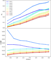 |
Fig. A.1. Mean evolution of βm parameter as a function of the cluster radial distance. Top panel: Mean evolution of βm for m = 1 to m = 9 as a function of the cluster radial distance. Bottom panel: Mean evolution of βm normalised by the sum of all order contributions |

Appendix B: Quadrupolar signature and ellipticity
As shown in the top right panel of Fig. 6, the quadrupole symmetry, β2, can be related to the ellipticity, ϵ. In Fig. B.1, we illustrate the distribution of quadrupolar ratios of hot gas and DM for all halos in the top panel and the distribution of their 2D ellipticities in the bottom panel. Both show similar behaviour and thus confirm that hot gas is more circular (less elliptical) than the DM distribution on average, in agreement with Velliscig et al. (2015), Donahue et al. (2016), and Okabe et al. (2018). Therefore, the quadrupolar ratio appears to be a good tracer of the ellipticity for both DM and hot gas components inside clusters.
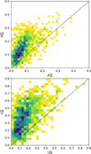 |
Fig. B.1. Distribution of quadrupolar ratio, β2 (top panel), and 2D ellipticity, ϵ (bottom panel), of dark matter and hot gas for our entire cluster sample. |
All Figures
|
Fig. 1. Stacked temperature-density diagrams for all gas cells around galaxy clusters and groups in IllustrisTNG, considering different radial apertures from cluster central regions R[R200]< 1 up to 4 < R[R200]< 5. |
| In the text | |
|
Fig. 2. Mean gas mass fraction profiles (see Eq. (7)) of the five different gas phases around all halos in our sample (top), only galaxy clusters (middle), and only galaxy groups (bottom). The radial boundary at which the hot gas phase is no longer dominant is shown by grey vertical lines and is about RHOT ∼ 0.91, 1.20 and 0.61 for the all groups and clusters, only clusters, and only groups, respectively. |
| In the text | |
|
Fig. 3. Stacked phase-space diagrams for all gas cells (left panels), only hot gas (middle panels), and warm-hot intergalactic medium (right panels). All groups and clusters are considered in top panels, only galaxy clusters (with M200 > 1014 M⊙ h−1) in the middle panels, and only galaxy groups (with M200 = [5−10] × 1013 M⊙ h−1) in the bottom panels. |
| In the text | |
|
Fig. 4. Illustration of different azimuthal symmetries as a function of harmonic orders, m. |
| In the text | |
|
Fig. 5. Illustration of dark matter (left), hot gas (middle), and WHIM (right) 2D projected distribution up to 5 R200 of one simulated galaxy cluster. The cyan ellipse on dark matter traces the ellipticity of the DM halo ( |
| In the text | |
|
Fig. 6. Distribution of βm parameter as a function of structural halo properties. Top left panel: distribution of βm dipole contribution (m = 1) as a function of the centre-of-mass offset. Top right panel: distribution of βm quadrupole contribution (m = 2) as a function of the 2D ellipticity of DM. Bottom left panel: distribution of βm quadrupole contribution (m = 2) as a function of the 3D ellipticity of DM. Bottom right panel: high azimuthal symmetries’ βm contribution (summing contributions from m = 3, 4, 5, 6, 7, 8, 9) as a function of the mass fraction of sub-structures. The mean profiles of β are shown by solid lines, and the error bars are the mean errors computed by bootstrap re-sampling. The β values for the DM distribution with apertures R < 0.5 × R200, R < 1 × R200 and R < 2 × R200, are, respectively, plotted in light, medium, and dark blue. The β values for 2D hot-gas distribution with R < R200 are plotted in red. In each panel, the number of objects used to compute the average in each x-axis bin (shown in grey dotted lines) is written above the figures in grey. |
| In the text | |
|
Fig. 7. Distribution of azimuthal symmetric excess β (as defined in Eq. (12)) as a function of the halo mass, inside clusters (R < R200) in the top panel and at cluster peripheries in (1 < R[R200]< 2) in the bottom panel. The mean profiles of β and their errors are shown in solid lines. The colours of points and lines represent different matter components: dark matter (black), hot gas (red), WHIM (orange), and all gas (light brown). In each panel, the number of objects used to compute the average in each bin of the x-axis (shown as grey dotted lines) is written above the figures in grey. |
| In the text | |
|
Fig. 8. Distribution of azimuthal symmetric excess β (as defined in Eq. (12)) computed at cluster peripheries in (1 < R[R200]< 2) as a function of the halo connectivity, for DM (black) and WHIM (orange). The mean profiles of β and their errors are shown as solid lines. The number of objects used to compute the average in each bin of the x-axis (shown with grey dotted lines) is written above the figures in grey. |
| In the text | |
|
Fig. 9. Distribution of azimuthal symmetric excess, β (as defined in Eq. (12)), computed inside clusters (R < R200) in top panels and at cluster peripheries (1 < R[R200]< 2) in bottom panels, as a function of different halo properties: level of relaxation on the left, mass-accretion rate in the middle, and formation redshift on the right. The mean profiles of β and their errors are shown in solid lines. The number of objects used to compute the average in each bin of the x-axis (shown with grey dotted lines) is written above the figures in grey. |
| In the text | |
|
Fig. A.1. Mean evolution of βm parameter as a function of the cluster radial distance. Top panel: Mean evolution of βm for m = 1 to m = 9 as a function of the cluster radial distance. Bottom panel: Mean evolution of βm normalised by the sum of all order contributions |
| In the text | |
|
Fig. B.1. Distribution of quadrupolar ratio, β2 (top panel), and 2D ellipticity, ϵ (bottom panel), of dark matter and hot gas for our entire cluster sample. |
| In the text | |
Current usage metrics show cumulative count of Article Views (full-text article views including HTML views, PDF and ePub downloads, according to the available data) and Abstracts Views on Vision4Press platform.
Data correspond to usage on the plateform after 2015. The current usage metrics is available 48-96 hours after online publication and is updated daily on week days.
Initial download of the metrics may take a while.