| Issue |
A&A
Volume 657, January 2022
|
|
|---|---|---|
| Article Number | A16 | |
| Number of page(s) | 17 | |
| Section | Stellar atmospheres | |
| DOI | https://doi.org/10.1051/0004-6361/202141623 | |
| Published online | 21 December 2021 | |
Variation of the stellar color in high-magnification and caustic-crossing microlensing events★
1
Department of Physics, Isfahan University of Technology,
Isfahan
84156-83111,
Iran
e-mail: s.sajadian@iut.ac.ir
2
Department of Physics, Chungbuk National University,
Cheongju
28644,
Republic of Korea
3
Centre for ExoLife Sciences (CELS), Niels Bohr Institute, University of Copenhagen,
Østervoldgade 5,
1350
Copenhagen,
Denmark
e-mail: uffegj@nbi.dk
Received:
24
June
2021
Accepted:
28
September
2021
Context. To a first approximation, the microlensing phenomenon is achromatic and great advancements have been achieved with regard to the interpretation of the achromatic signals, leading to the discovery and characterization of well above 100 new exoplanets. At a higher order accuracy in the observations, microlensing has a chromatic component (a color term) that has thus far been explored to a much lesser extent.
Aims. Here, we analyze the chromatic microlensing effect of four different physical phenomena, which have the potential to contribute key knowledge of the stellar properties that is not easily achievable with other methods of observation. Our simulation is limited to the case of main-sequence source stars.
Methods. Microlensing is particularly sensitive to giant and sub-giant stars near the Galactic center. While this population can be studied in short snapshots by the largest telescopes in the world, a general monitoring and characterization of the population can be achieved by use of more accessible medium-sized telescopes with specialized equipment via dual-color monitoring from observatories at sites with excellent seeing. We limit the results of this study to what will be achievable from the Danish 1.54 m telescope at La Silla observatory based on the use of the existing dual-color lucky imaging camera. Such potential monitoring programs of the bulge population from medium-sized telescopes include the characterization of starspots, limb-darkening, the frequency of close-in giant planet companions, and gravity darkening for blended source stars.
Results. We conclude our simulations with quantifying the likelihood of detecting these different phenomena per object where they are present to be ~60 and ~30% for the above-mentioned phenomena when monitored during both high-magnification and caustic crossings, respectively.
Key words: gravitational lensing: micro / instrumentation: photometers / methods: numerical / planets and satellites: general / starspots / stars: early-type
Full Table A.1 is only available at the CDS via anonymous ftp to cdsarc.u-strasbg.fr (130.79.128.5) or via http://cdsarc.u-strasbg.fr/viz-bin/cat/J/A+A/657/A16
© ESO 2021
1 Introduction
According to Einstein’s theory of general relativity, the light path of a background star (the source) is bent while passing through the gravitational field of a foreground object (the lens star, or any other massive object). The calculation of this bending angle is (Einstein 1936):
 (1)
(1)
where Ml is the mass of the lensing object, b is the impact parameter (i.e., the minimum distance of a light ray and the lensing object), G is the gravitational constant, and c is the speed of light. Hence, in a lensing phenomenon, the bending angle does not depend on the wavelength of the light. A gravitational red and blue shift of the light does occur, because of the component of the gravitational force parallel to the light path, but it is symmetric in direction while the light approaches and moves away from the lensing object, so the wavelength before and after the passage remains the same.
In a lensing phenomenon, two or more distorted images are formed and their angular distance depends on the physical lens and source distances from the observer and on the mass of the lens. When the lens and source stars are inside the Galactic disk and bulge, respectively, the angular distance of the images is less than a milliarcsecond, which is too small tobe resolved. This kind of lensing is known as gravitational microlensing (Liebes 1964; Chang & Refsdal 1979; Paczynski 1986).
One important quantity in microlensing events that can be inferred from observations is the magnification factor of the source flux relative to its value at the baseline, namely, A(t). In the point-sourceapproximation, it is given by (Einstein 1936):
 (2)
(2)
where, u(t) is the angular lens-source distance normalized to the angular Einstein radius θE, which is the angular radius of the ring of the images for perfect alignment (see, e.g., Schneider et al. 1992; Gaudi 2012).
In a more realistic treatment of the microlensing phenomenon, where the source star is considered to be of a finite size, rather than a point, each infinitesimally small area of the source star is usually treated as displaying the same color. This results in a realistic evaluation of A(t), but still results in an achromatic magnification factor. This approximation has been very successful for characterizing even the minute details of exoplanets orbiting the lensing stars, however, a real star certainly does not exhibit a single color over its surface; thus, during a lensing phenomenon various elements of the source star will be amplified with various strengths as a function of time, depending on their position on the source surface. In reality, the resulting magnification light curve will therefore be color-dependent (i.e., chromatic).
These variations are small compared to the general magnification, but they contain important information about the source stars that are not easily obtainable in other ways. In the text above, we mention various such systematic color variations and we show in the following sections that these are measurable for medium-sized ground-based telescopes. Of particular importance is the color variations due to close-in giant planets transiting the source star during the lensing. Generally, there are two main channels for detecting exoplanets through microlensing observations: (i) detecting gravitational perturbations on the source brightness due to exoplanets orbiting lens objects (see, e.g., Mao & Paczynski 1991; Gould & Loeb 1992; Tsapras 2018) and (ii) detecting perturbations on the source brightness profiles or their astrometric motions while lensing due to giant planets orbiting them (e.g., Graff & Gaudi 2000; Rahvar & Dominik 2009; Bagheri et al. 2019). Microlensing measured from dual-color instruments on medium-sized telescopes, such as the Danish 1.54 m telescope at ESO’s La Silla observatory in Chile (Harpsøe et al. 2012; Skottfelt et al. 2015), will (to the best of our knowledge) be the only viable way of obtaining statistics on the exoplanet population of stars near the Galactic center, thereby adding important new information to the search for answers about the dependence of exoplanetary frequencies on the galactic environment. Ongoing high-magnification (hereafter HM) and caustic-crossing (hereafter CC) microlensing events have been (and continue to be) followed up by the Danish telescope since 2008 (Dominik et al. 2008). In several cases, its observations made betterresolutions of the planet signatures and more precise characterizations of these planets (see, e.g., Udalski et al. 2018; Han et al. 2018; Ryu et al. 2018; Li et al. 2019; Street et al. 2019; Hirao et al. 2020; Kondo et al. 2021).
The chromatic change of limb-darkened source stars in HM microlensing events was first investigated by Valls-Gabaud (1998). At the time, the chromatic changes of limb-darkened source stars in HM and CC microlensing events were studied based on the blending (BL) effect, as described in Han et al. (2000a); Han & Park (2001); Pejcha & Heyrovský (2009). The chromatic variations of highly blended source stars during microlensing events can reveal their types (Tsapras et al. 2019). Such measurements are done by multiband follow-up microlensing observations with the ROME/REA project. More recently, the chromatic deviations in HM or CC microlensing events due to radially and non-radially pulsating source stars were studied extensively (Sajadian & Ignace 2020a,b; Sajadian et al. 2021). All of these studies emphasize the importance of detection and characterization of chromatic deviations during microlensing events.
In this work, we extend these previous studies by considering more realistic models for the limb-darkening (LD) effect for different types of source stars based on their atmospheric models and including the blending effect. Here, the chromatic effects are most accurately studied during HM, whereas CC features are best considered when the relative differences between the magnification of different parts of the source star is largest. We therefore simulated HM and CC microlensing events toward the Baade’s window of blended source stars with variable color over their surfaces and studied the resulted chromatic perturbations. Five causes for variable source star surface color studied below are the BL, LD, close-in giant planet companions (CGPs), stellar spots (SS), and finally gravity-darkening (GD) for hot stars, which are described separately in Sects. 2–6, respectively. In the last section of the paper (Sect. 7), we summarize our conclusions.
2 Blending effect
Microlensing observations have typically been done toward the Galactic bulge. In these directions, the column number density of stars is high, which leads to the source light being blended with other close stars in the so-called blending effect (see, e.g., Di Stefano & Esin 1995; Smith et al. 2007). To evaluate this effect, we determined the average cumulative number of stars in a given direction and distance, as follows:
 (3)
(3)
where, (lG, bG) specify the Galactic longitude and latitude, D is the distance which changes from zero to Ds (the source position with respect to the observer), and ΩPSF is angular size of the source PSF (point spread function). The summation is done over different Galactic structures including the Galactic thin and thick disks, the bulge, and the stellar halo. Here, ρi and  represent the stellar mass density and the average mass of these Galactic structures, respectively. Toward a given direction, the number of blending stars is
  , where δNb is determined from a normal distribution with the width
  . For each of these blending stars, we determine its flux in a given filter,
  , using the Galactic Besançon model (Robin et al. 2003, 2012). The index F refers to the adopted filter and F ∈ UBV RI. Further explanation can be found in Moniez et al. (2017); Sajadian & Poleski (2019); Sajadian (2021).
Accordingly, the observing magnification factor by considering the blending effect is evaluated by:
 (4)
(4)
where,  is called the blending parameter and
  is the total flux due to all blending stars. A(t) is the magnification factor of the source star. For point-like source stars in single microlensing events, the magnification factor is evaluated by Eq. (2). By considering finite-size of the source star, this magnification factor deviates from its simple model which will be studied in the next sections.
The blending parameter is unity if there are no blending stars. It also depends on the adopted filter. Hence, during a microlensing event, the blending effect makes chromatic perturbations. We measure the variation in the stellar color during a microlensing event via:
![\begin{eqnarray*}\Delta C_{FF\prime}\,{=}\,C(t)-C_{\textrm{base}}\,{=}\,-2.5 \log_{10}\left[\frac{A_{\textrm{b}, ~{F}}}{A_{\textrm{b}, ~{F}^{\prime}}}\right],\end{eqnarray*}](/articles/aa/full_html/2022/01/aa41623-21/aa41623-21-eq11.png) (5)
(5)
where  is the variation in the stellar color during a microlensing event with respect to the baseline, F, F′∈ UBV RI, and
  is the apparent stellar color, namely, the difference of the stellar apparent magnitude in filters F, F′. Here, we have
 ![$m_{F}\,{=}\,m_{\textrm{base},~{F}} -2.5 \log_{10}\left[A_{\textrm{b},~{F}}\right]$](/articles/aa/full_html/2022/01/aa41623-21/aa41623-21-eq14.png) and
and  .
.
In order to evaluate the above chromatic perturbations due to a blending effect, we simulate a large number of microlensing events toward the Galactic bulge. This is due to the fact that most of today’s microlensing observations are done in these directions, namely, toward the Baade’s window, for instance (e.g., Paczynski et al. 1999). Yet in real observations, highly blended microlensing events are eliminated (see, e.g., Mróz et al. 2017, 2019), because the high blending effect makes for a more severe degeneracy when modeling microlensing events (see, e.g., Smith et al. 2007; Mróz et al. 2020; Sajadian 2021). Hence, in the simulations, we excluded the highly blended events with bI < 0.2. By simulating microlensing events toward the Baade’s window with the coordinate (lG, bG) = (1°, − 4°), the average blending parameters in different filters are estimated as  , respectively. Thus, the blending parameter depends, in fact, on the observing directions.
In considering these blending parameters, variations in the stellar colors V -I and B-R are plotted in Fig. 1 versus the magnification factor. Based on this plot, we list some key points here.
- (i)
The blending-induced chromatic variations increase according to the enhancement of the magnification factor. For a magnification factor higher than ≳40, their increasing slopes decrease and tend toward zero. However, the maximum chromatic perturbations take place at the magnification peak.
- (ii)
The time scale of the chromatic perturbations due to blending effect is on the order of tE (the Einstein crossing time that determines the time scale of a microlensing event). This is because when the magnification factor is enhanced from unity, the chromatic perturbations increase as well.
- (iii)
For transit microlensing events, the magnification factor (by considering the finite-source effect) remains almost constant as the lens object is passing over the source disk, which results in constant chromatic perturbations.
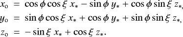
In Fig. 2, we show four examples of HM and CC microlensing light curves considered with the blending effect. In these plots, the magnification factors in the filters UBV RI are plotted with magenta, blue, green, orange, and red colors, respectively. In order to calculate the magnification factor in binary microlensing events, we used the RT -model1 developed by V. Bozza (Bozza et al. 2018; Bozza 2010; Skowron & Gould 2012). In these light curves, the time of closest approach defines time zero. The residual parts show the variation in the stellar colors V -I (black solid curves) and B-R (gray solid curves) in unit of magnitude (Eq. (5)). In the top panels, the right-hand insets show the source disk (blue circles) and the lens trajectory (black lines), both projected on the lens plane. In the bottom panels (binary CC microlensing events), the right-hand insets represent the caustic (brown curve) and the source trajectory projected onto the lens plane (black line). As mentioned above, the variation in these chromatic perturbations around the magnification peak is very gradual.
In order to study the detectability of the resulted chromatic perturbations, we generated synthetic data points corresponding to observations with the lucky imaging (LI) camera at the Danish 1.54 m telescope at ESO’s La Silla observatory in Chile. In Fig. 2, the data points in the I-band are shown as red points on the magnification light curves (top parts) and the resulting perturbations in the stellar color V -I (given by Eq. (5) and in magnitude units) are plotted as cyan points on the residual parts.
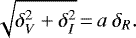
Some scatters were added to the data points given in filter F by using a Gaussian distribution with a width equal to the error bars, δF. In Appendix, we explain how to determine the error bars of the synthetic data points taken with the LI camera. Subtracting the two magnitudes, in the F, F′-bands, from each other results in the following change in the error bar in the stellar color:  . The cadence between data points from on-going microlensing events, taken by this camera, depends on the magnification factor and can change in the range τ ∈ [2 min, 2 h], as explainedin Dominik et al. (2010); Sajadian et al. (2016).
The parameters of these light curves are given in Table 1. In this table, in the last column, the value of Δχ2 is given as  , which is the difference between the χ2 values from fitting the real models and the baseline measurement for the source color versus time.
Comparing Figs. 2a,b, it can be seen that the higher blending effects lead to greater chromatic deviations. However, the blending effect decreases maximum magnification factors and, effectively, restricts the achievable S/N. Hence, detecting these chromatic perturbations in highly blended microlensing events is difficult, unless the source star at the baseline is very bright.
In order to evaluate the detectability and properties of the chromatic perturbations in HM microlensing events with the LI camera, we generated a sizable ensemble of these (HM and CC) events. For simulating HM events, we choose the lens impact parameter uniformly from the following range: [0, 0.01] (which constitutes around one per cent of all microlensing events). We simulate their light curves over a two-day time interval around their peaks. The start time of simulating data points is chosen uniformly from the range of [0, 24] h and we assume that the observations can be done over 6.5 h in a day. For simulating binary microlensing events, we only simulated the CC features and generate the synthetic data points in a two-day time interval around them.
We considered Δχ2 > 100, 200 as the detectability criterion for the chromatic perturbations with low and high sensitivities in the simulated light curves. The results from this Monte-Carlo simulation and other simulations, which will be explained in next sections, are summarized in Table 2. In this table, ϵh and ϵl are the LI efficiencies for detecting chromatic perturbations with high and low sensitivities. These chromatic perturbations are potentially generated due to different physical effects or their combination (identified with the symbol &), as specified in different rows of the table. Two next columns of this table also represent average values of maximum chromatic deviations in detectable (simulated) microlensing events. The next column reports the average of the lens impact parameter of detectable microlensing events. In addition, f100, f200, and f500 represent the fraction of the simulated events with detectable chromatic perturbations, and with the maximum magnification factor higher than 100, 200, and 500, respectively. The last column, marked No., declares the number of simulated events with detectable perturbations.
Accordingly, the chromatic deviations attributed to the blending effect can be detected rather in HM microlensing events (with the maximum magnification higher than 100) than CC binary events. In the next section, we add another source for chromatic perturbations which is the LD effect.
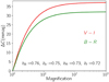 |
Fig. 1 Variation in the stellar colors V -I (red) and B-R (green) versus the magnification factor due to the BL effect. The adopted blending parameters, given in the figure, are the average of blending parameters for simulated microlensing events toward the Baade’s window, with the coordinate (lG = 1°, bG = − 4°), by excludinghighly blended events with bI < 0.2. |
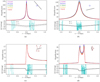 |
Fig. 2 HM and CC microlensing light curves of blended source stars in the passband filters UBV RI, are shown by magenta, blue, green, orange, and red colors, respectively. The perturbations in stellar colors V -I and B-R during the lensing effect are shown in the residual parts by solid (black and gray) curves, respectively. The source star parameters are listed in Table 1. The synthetic data points by the LI camera at the Danish telescope in the I-band are shownwith red filled circles. The corresponding data points over the residual parts (related to the V -I color) are plotted by cyan filled points. In the two top panels, each right-hand inset shows the source star (blue circle) and the lenstrajectory (black line) both projected on the lens plane. In the bottom panels, each right-hand inset shows the caustic curve (brown curve) and the source trajectory (black line) projected onto the lens plane. |
LI efficiencies for detecting chromatic perturbations in HM single and CC binary microlensing events and the properties of these events.
3 Limb-darkening effect
The gradual decrease in brightness of the stellar disks from center to limb, as seen by the observer, is called limb-darkening. The line of sight through the atmosphere is larger on the limb than at the center of the disk and, hence, the light from the limb is dominated by higher layers in the atmosphere than the light reaching the observer from the center of the disk. Since the higher layers are generally cooler than the deeper layers in the atmosphere, the light from the limb is generally more redder than the light from the center. In other words, photons can escape the stellar photosphere when the optical thickness is about one for a given wavelength, so photons observed in the center of a stellar disk come from a deeper layer of the stellar atmosphere than photons observed toward the limbs.
The detailed calculation of this dependency requires the modeling of the stellar atmospheres and a numerical solution to the transfer equations (Code 1950; Chandrasekhar 1960). Such simulations were done by P. Harrington in 20172 (Harrington 1970, 2015, 2017), who considered several models of the stellar atmospheres, such as the MARCS models for cool stars with an effective temperaturerange of [2500, 8000] K and log[g] = 3, 3.5, 4, 4.5, 5 (Gustafsson et al. 2008; Van Eck et al. 2017), the TLUSTY models for hot stars (Lanz & Hubeny 2003, 2007) and the STERNE and KURUCZ models for stars within the temperature range [8000, 15000] K (Kurucz 1993; Castelli & Kurucz 2003). Accordingly, he offered the polarized and total emergent continuum radiation at different wavelengths versus  , where ρ = R∕R*, R is the radial distance over the source disk from its center and R* is the stellar radius.
Using his output, we integrate the emergent radiation, B(μ, λ), over the wavelength by considering the transmission function for the standard filters F ∈ UBV RI, as follows:
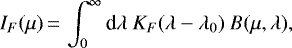 (6)
(6)
where KF(λ − λ0) is the transmission function for the filter under consideration. For four stars with effective temperatures of 3000, 6000, 12000, and 30000 K, we plot their normalized intensities in the different filters UBV RI with magenta, blue, green, orange, and red colors versus μ in Fig. 3. These plots show the dependence of the stellar radiation on the used filters. All of these curves have a similar trend, with their largest value at the source center and decreasing slowly from center to limb. For hotter stars the higher emergent intensities occur at shorter wavelengths. In order to study for what kind of stars the contrast of stellar radiation in different filters is highest, we fit linear functions to the stellar radiation and compare their coefficients.
Generally, for the emergent radiation versus μ, a very simple and known function is considered, which is:
![\begin{eqnarray*}I_{F}(\mu)\,{=}\,I_{0,~F} \Big[1- \Gamma_{F} (1- \mu) \Big],\end{eqnarray*}](/articles/aa/full_html/2022/01/aa41623-21/aa41623-21-eq21.png) (7)
(7)
where ΓF is the so-called LD coefficient which depends on the adapted filter. We estimate ΓF for the standard filters UBV RI for the differenttypes of stars with different effective temperature and surface gravity and plot the results in Fig. 4. The LD coefficients in the UBV RI filters are shown by magenta, blue, green, orange, and red colors, respectively.
The emergent radiation curves do not behave in a linear fashion, especially for μ ≲ 0.1 (see Fig. 3). Hence, the linear function given by Eq. (7) mostly describes the emergent radiation for μ ≳ 0.1. The largest contrast between the LD coefficients in different filters happens for stars with intermediate temperatures around T ~ 4000–5000 K. Changes in surface gravity do not have a significant impact on the emergent radiation contracts between different filters due to the corresponding low sensitivity of the absorption coefficients on gravity.
Dependence of the emergent radiation in the different filters under consideration causes the stellar color to change in microlensing events, while the lens is passing over (or close to) the disk of the source star. In order to study the variation in the stellar color, we inset the lensing magnification factor in the stellar flux integration over the source disk as:
 (8)
(8)
where, (x, y) is the location of each element over the surface of the source star, so that  , (ux, uy) is the location of that element with respect to the lens position projected on the lens plane and normalized to the Einstein radius. If there is no blending effect, the magnification factor of a limb-darkened source star in the adopted filter F is given by:
 (9)
(9)
where,  is the stellar flux measured in the filter F at the baseline. We expect that the largest variation in the stellar colors due to LD effects occurs during HM microlensing events (especially when the lens is directly transiting the source disk) and in CC binary microlensing events. This is due to the fact that when the lens impact parameter is larger than the source radius, or the source is far from the caustic line, the finite-source effect is small and all elements over the source disk have almost the same magnification factor. By including the blending effect, the magnification factor becomes:
 (10)
(10)
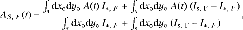
Four examples of HM and CC microlensing light curves from limb-darkened and blended source stars are plotted in Fig. 5. Some details about these plots can be found in the caption of Fig. 2. In these light curves, the right-hand colored schemes represent the stellar surface brightness. In the residual parts, the perturbations in stellar colors V -I (black) and B-R (gray) during the lensing effect, due to LD and BL effects are shown by dashed curves, respectively. The corresponding chromatic perturbations due to only the BL effect are shown by solid curves. The parameters of the source stars responsible for the light curves are listed at Table 3.
We see from these plots that the peak and width of the microlensing light curves depend on the LD coefficients and, as a result, also the filter under consideration. When the lens is passing very close to the source center (u0 ≃ 0), the value of the magnification peak is:
 (11)
(11)
where, ρ* is the projected source radius normalized to the Einstein radius. The level of variation in the magnification peak in different filters is scaled by  , namely, the smaller the projected radii of the source stars, the larger the variations in the magnification factor in the different filters. This magnification peak is an increasing function of ΓF. We see from Fig. 4 that for a given source star, the coefficient of ΓF is smaller at longer wavelengths, which results in more flattened light curves. However, if the lens is crossing close to the source edge, for instance, in a non-transiting event, the magnification peak is maximized in the I-band.
In addition to the magnification peak, the width of the light curve depends on the passband filter as well. The full width at half maximum (FWHM) of a microlensing light curve (Δt) is given by
 (12)
(12)
![\begin{eqnarray*}D\,{=}\,\frac{4-A_{\textrm{m}}^{2} + A_{\textrm{m}}\sqrt{A_{\textrm{m}}^{2}-4}}{A_{\textrm{m}}^{2}/2-2}. \\[-13pt] \nonumber\end{eqnarray*}](/articles/aa/full_html/2022/01/aa41623-21/aa41623-21-eq30.png)
Here, D decreases with increasing value of the magnification peak. Therefore, in transit microlensing events, the magnification peak decreases and its width increases (i.e., the light curve is more flattened) in longer wavelengths. These two factors cause the chromatic perturbations of LD effects on microlensing light curves to be symmetric with respect to the time of closest approach, t0, and also to maximize the perturbation at the time of closest approach.
The LD-induced chromatic perturbations are highlighted during CC features as well. We note that during caustic crossings these chromatic perturbations have the same tendency as during the high magnification peak (see the residual part of 5d); but during the caustic crossing, the perturbations are not symmetric (with respect to the time the source center passes the caustic curve) unless the source trajectory passes from the binary axis normally. The maximum perturbation happens when the source edge is on the caustic curve and the source center is beyond it (i.e., while the magnification factor is sharply increasing). At that time, the magnification factor at longer wavelengths is higher than at shorter wavelength.
The time scale of the LD-induced chromatic perturbations is on the order of t* = tE ρ*, namely, the source radius crossing time. From simulations, we note that the events with the shortest t* are least suitable for measurements of their chromatic perturbations.
The timescale of BL-induced chromatic deviations is of order tE, which is longer than t*. Additionally, these BL-induced deviations remain approximately constant while the lens is crossing the source disk. As a result, in the residual parts of Fig. 5, the difference between solid and dashed curves are highlighted only when either the lens is crossing the source disk or the source disk is passing the caustic lines. So, the BL-induced chromatic deviations can be subtracted from the chromatic curves. This helps us to study the chromatic deviations due to any possible perturbations in the stellar brightness profiles. In this sense, the BL effect will not make degenerate chromatic perturbations with the LD effect.
For transit microlensing events, the chromatic perturbations due to only the LD effect can reach to 0.025–0.04 mag close to the peak of the light curve, which is detectable with LI camera at the Danish 1.54 m telescope. For non-transit HM (single) microlensing events in which the lens passes very close to the source edge, u0 ≃ ρ*, the LD-induced chromatic perturbation at the time of the closest approach can reach ~ 0.01 mag, which is, again, detectable with the LI camera (see Fig. 5b).
When CC features are seen, the LD-induced chromatic perturbations can reach to 0.05–0.1 mag (see Fig. 5c), but the duration of such high signal is generally too short (it happens when the source edge is entering the caustic and its center is out of it). If the source star is moving parallel to the caustic curve or when the source size is comparable with the caustic size, the timescale of the chromatic perturbations increases and their chromatic perturbations can be measured. Another way to detect such short-duration perturbations is improving the observing cadence. From our simulation of HM and CC microlensing events, we note that the LD-induced perturbations in B-R are always larger than those in V -I.
We perform a Monte-Carlo simulation from HM and CC microlensing events from limb-darkened and blended source stars toward the Baade’s window. We find that for the HM events, the probabilities of detecting the chromatic perturbations with low and high sensitivities are 62 and 50%, respectively.For CC binary microlensing events, the probabilities of detecting the chromatic perturbations with the LI camera are 31% (low sensitivity) and 22% (high sensitivity) in each CC feature (as reported in the rows of Table 2 labeled by BL & LD). Generally, during CC, magnification factors are not as high as for HM microlensing events. That causes larger error bars for data taken during CC than those taken in HM events. The dependence of error bars to the stellar apparent magnitudes is shown in Fig. A.1.
Accordingly, if the Danish 1.54 m telescopein each observing season covers the magnification peaks of ~ 10 HM microlensing events (withu0 < 0.01) and ~10 CC features in binary events during two-day time intervals around their peaks3, we can therefore expect to be able to detect the chromatic perturbations for about seven events per observing season even within our standard priority of events.
Generally, the brighter source stars in longer microlensing events are the most suitable candidates for measuring their chromatic perturbations (see, Fig. 5a), for instance, the events of red giant source stars with large ρ* values. These stars are intrinsically bright and because of their large radii, their t* values increase. In out simulations, we in fact used the emergent radiations for cool stars with log [g] ≥ 3.0 as developed by P. Harrington, corresponding to main-sequence stars. For red giant stars, the LD effect is stronger (see, e.g., Zub et al. 2011), which makes them the most suitable candidates for chromatic measurements.
An important conclusion from our simulations is that if there are several sets of data points for a given microlensing event taken by different telescopes with different filters, then for these sets of data, the resulting light curves will be slightly different because the related LD coefficients and blending parameters are different. Considering the same LD coefficients for all data sets generates some extra noise in the data (around the peaks) with respect to the best-fitted model. We note that the conversion of the magnitudes of the different telescopes and filters to a common filter system (before finding the best-fitted model) does not solve this problem because the discrepancy is time-dependent between the magnified magnitudes in different filters, whereas the conversion relations for the magnitudes in different filters are applicable to the unperturbed baseline data. In the next section, we study another source for chromatic perturbations, namely, close-in giant planet companions around the microlensing source stars.
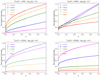 |
Fig. 3 Emergent radiation intensities for four stars with different temperature and the surface gravity values versus μ in the standard filters, UBV RI, as shown with magenta, blue, green, orange, and red curves. |
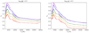 |
Fig. 4 LD coefficients, ΓF, in different filters F, ∈ UBV RI (shown with magenta, blue, green, orange and red colors, respectively), for stars with different effective surface temperatures and two values of the surface gravity (given at the top of the plots). |
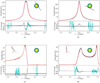 |
Fig. 5 HM and CC microlensing light curves of limb-darkened and blended source stars are plotted. Details are similar to those in Fig. 2. The lensing parameters are listed in Table 3. In the residual parts, the perturbations in stellar colors V -I and B-R during the lensing effect due to LD and BL effects are shown by dashed (black and gray) curves, respectively. The corresponding chromatic BL-induced perturbations are shown by solid curves. The right-hand insets (colored schemes) represent brightness profiles over limb-darkened source disks. |
4 Close-in planetary systems
Close-in giant planet companions (CGPs), or so-called hot Jupiters, have been discovered in abundance during the Kepler mission and through transit or radial velocity measurements from the ground (Borucki et al. 2010). Hot Jupiters are Jupiter-like planets located at the distance range [0.01, 0.1] au from their parent stars. Their orbits are most often tidally locked and their orbital periods are ~ 3–10 days. These objects perturb their host star brightness but also their color. These faint and small color distortions are optimally observable at long wavelengths, that is, the infrared, in HM or CC microlensing events through photometric or polarimetric observations (Graff & Gaudi 2000; Sajadian & Rahvar 2010; Sajadian & Hundertmark 2017). This channel of exoplanet detection is parallel to the main channel of planet detection in microlensing events where the gravitational effect of a planet in the lensing system affects the light path of an image of the source star (see, e.g., Mao & Paczynski 1991; Beaulieu et al. 2006; Gaudi 2012). In this section, we study how CGPs orbiting the source star can make detectable chromatic perturbations in HM and CC microlensing events.
For simulating close-in planetary systems as microlensing sources, we applied the following assumptions: (i) the planet orbit is circular (its eccentricity is zero); (ii) the planet temperature is uniform over its surface; (iii) each source star is orbited by a CGP (such that the statistics becomes per CGP); (iv) the source star acts as a black body and its radiation is thermal and specified according toits effective temperature.
For projection of the planetary orbit onto the plane of the sky, we use an inclination angle, i, which is the angle between the orbital plane and the plane of the sky. If i = 0 the planetary orbit will be circular as seen by the observer. The phase angle, β, that is, the angle between line of sight to the observer and the host source star as seen by the planet, indicates the position of the planet with respect to the source center. If 90° < β < 180°, the planet is transiting in front of the source surface and can block the source brightness and for 0 < β < 90° the planet is passing behind its host star and its light can be blocked by host star. To estimate the planet radiation, we consider two components, thermal and reflected ones. All details about calculating these radiations can be found in Sajadian & Hundertmark (2017).
In Fig. 6, four examples of HM and CC microlensing events of close-in planetary systems are shown. The insets represent the planetary orbits projected onto the sky plane (green curves), the host stars and planets (blue and red circles), and the lenstrajectory (black solid lines). For the host stars we consider the LD and BL effects as well. The chromatic perturbation in the source colors by considering only LD and BL effects are shown by solid (black and gray) curves in the residual parts. The total chromatic perturbations due to the source stars and their CGPs are shown by dashed (black and gray) curves. The parameters of these light curves are reported in Table 4. We note some key points from these light curves.
- (i)
The CGPs make small extra perturbations in the stellar color curves which mostly happens when the lens is passing very close to planets (e.g., Figs. 6a,b).
- (ii)
The planet-induced perturbations are strongest in the I-band. Hence, the planet-induced perturbations are larger in the stellar color V -I than B-R (e.g., see Fig. 6b).
- (iii)
The edge-on planetary orbits, with the inclination angle is i ~ 90°, create greater chromatic perturbations, namely, the main source for chromatic perturbation for the source star in these systems is the occultation of the stellar brightness by the planet transit.
By assuming Δχ2 > 100, 200 as the detectability criteria with low and high sensitivities, we conclude that the detection probabilities for chromatic perturbations in HM microlensing of close-in planetary systems is 64 and 53%, respectively. We note that by considering only LD and BL effects for the source star this probability is 50–62%, thus, CGPs improve the detection probability of chromatic perturbations by ~ 2%. In binary CC microlensing events, the probability of detecting CGPs is 23–32% and reported in Table 2. In the next section, we consider one stellar spot for each source star which are highly magnified and study the characteristic and statistic of the resulting chromatic perturbations.
5 Stellar spots
The effects of stellar spots (SS) in microlensing light curves have been studied extensively in several references. Here, we offer a brief review. The detection of stellar spots in single and binary microlensing events was studied by Heyrovský & Sasselov (2000); Han et al. (2000b) and they reported the spot-induced deviations for spots with radii smaller than 0.2 R* can reach up to 2%. Detecting stellar spots in different wavebands as a function of the spot temperature was also investigated in Hendry et al. (2002). Additionally, Hwang & Han (2010) has also studied the detection and characterization of stellar spots in the next generation of microlensing observations with short cadence and concluded the size and the location of the stellar spots are measurable through such observations. Polarimetry follow-up observation from HM microlensing events of red giant source stars is an alternative approach for illuminating stellar spots and even measuring the stellar magnetic field. In that case, stellar spotsperturb the polarimetry curves (Sajadian 2015). Intrinsic rotation of the source star around its axis causes the location of its stellar spot to vary while the lens is transiting the source surface in HM microlensing events. Accordingly, stellar rotation alters the spot-induced perturbations on microlensing light curves (Giordano et al. 2015).
Here, we study the chromatic perturbations due to stellar spots in HM and CC microlensing events. For simulating stellar spots, we follow the approach introduced in Sajadian (2015) and consider four relevant parameters. Here, fV is the ratio of the stellar brightness over the spot to its value at the source center in V -band without spot, θ0 is the enclosing angle to the stellar spot as measured from the source center and with respect to the axis passing from the spot center. It determines the spot area. We also need two angles, ξ and ϕ, to project the stellar spot on the sky plane. In the projection process, there are two coordinate systems: the stellar coordinate system (x*, y*, z*) and the observer one (xo, yo, zo). We set the spot on the stellar pole (in the stellar coordinate system) with θ* < θ0. One can convert the first coordinate system to the second one by two consecutive rotations, around y* -axis by the angle ξ and then around z*-axis by the angle ϕ, as:
 (14)
(14)
The points with zo > 0 are detectable by the observer and make the projected stellar disk on the sky plane. We consider only one spot foreach source star. For each spot the enclosing angle is chosen uniformly from the range [5, 20] deg. The fraction fV is also taken randomly as fV ∈ [0.1, 0.7]. Two projection angles are selected randomly from the range [5, 85] deg. We consider the LD and BL effects for each source star and add one spot in a random place over the source surface.
The overall magnification factor of the spotted source star in the adopted filter,  , can be given by:
 (15)
(15)
where the indexes s and * refer to the disks of the spot and the source star (both projected on the sky plane), respectively. I*, F and Is, F are the intensities of the source star considering the LD effect and its spot in the fiter F, respectively. A(t) is the magnification factor of each element with the coordinate (xo, yo). If we assume constant values for the intensities, I*, F and Is, F, and ignore the LD effect, the overall magnification factor can be simplified as follows:
 (16)
(16)
where, A*(t) and As(t) are the magnification factors of the whole source star and its spot, respectively, α is the ratio of the spot area to the source area (both projected on the sky plane). We note that although fF ∈ [0, 1], α has very small values, which makes the factor α(1 − fF) be very small. fF depends on the waveband and therefore generates SS-induced chromatic perturbations in HM and CC microlensing events, evenif we ignore the LD effect of the source star. By adding the BL effect, the magnification factor is:
 (17)
(17)
Four examples of the microlensing light curves from spotted source stars are shown in Fig. 7. The parameters of these light curves are given in Table 5. For the source stars, the LD and BL effects are considered as well. In the residual parts, we plot the perturbations in the source color V -I (black) and B-R (grey) due to the LD and BL effects (solid curves) and LD, BL plus stellar spots (dashed curves). The spot size depends on both projection angles and the enclosing angle. Right-hand insets represent the brightness profiles of the spotted source star and the lens trajectories projected on the source plane (solid black lines). We note the following key points from the figures.
- (i)
Spots make asymmetric chromatic perturbations with respect to time of the closest approach, unless the spot is exactly on the source center (which is rare) or the lens-spot distance minimizes at t0. We note that the LD and BL effects itself causes symmetric perturbations.
- (ii)
If the lens is crossing the spot disk, then generally the whole magnification decreases, but at the same time the spot acts as an extra, faint and cooler source star, which affects the I-band, so that the spot significantly perturbs the light curve in the I-band filter. In that case, a significant perturbation is made in the V -I color, whereas the LD effect of the source star is mostly higher in B-R band, see Fig. 7a. In these cases (i.e., when the lens transits the spot surface), the chromatic perturbations in the V -I stellar color can reach 0.07 mag.
- (iii)
If the lens passes close to the stellar spot but not over its surface, the spots make perturbations in the chromatic curves due to limb-darkened and blended source stars. These perturbations for the spots located at the source edges are too short to be observed.
- (iv)
Generally, the spot makes the chromatic perturbations in V -I and B-R take different forms and their symmetry with respect to the time of the closest approach is thus broken.
- (v)
As seen from Fig. 7a, the spot-induced perturbations in microlensing light curves can be similar to planetary ones. In that case, one possible test to resolve these degenerate solutions is to measure the stellar color. If it changes with time, the perturbation source should be a stellar spot, otherwise it is likely to be a planet around the lens object.
- (vi)
If the position of the stellar spot is projected on the center of the source disk, it can make similar and degenerate magnification curves and chromatic perturbations to that made by a transiting giant planet. Because they make similar perturbations for the stellar brightness profile.
- (vii)
The time and duration of the perturbation depends on the spot location. If the spot is on the stellar edge, its size after projection on the source disk will usually be very small, which will result in a very short-duration perturbation. We note that if the observing cadence is improved during caustic crossing, the probability for detecting such perturbations increases significantly.
In order to study the detectability of the chromatic perturbations in HM microlensing events of the limb-darkened, blended, and spotted source stars, we simulated an ensemble of these events and assumed that when Δχ2 > 100, 200 the chromatic perturbations are detectable with low and high sensitivities. We conclude that these perturbations are measurable in ~ 62.7, 51.0% of the events when observed by the LI camera near their peaks. One example is shown in Fig. 7a. In binary CC events, these probabilities are 36, 27%.
According to the results of the simulation in the previous section, the spot-induced perturbations improve the detectability by ~ 0.5, 5.0% in HM and CCevents, respectively. The stellar spots most often pass from the caustic curves during CC features (see, bottom panels of Fig. 7), whereas the probability of crossing the spot disk by the lens in HM events is low.
In the next section, we assume the microlensing source stars are hot and early-type ones with gravity-darkening effects and we study their chromatic perturbations.
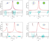 |
Fig. 6 HM and CC microlensing light curves of limb-darkened and blended source stars are plotted, but we additionally consider a close-in giant planet around each source star. Details are similar to those in Fig. 5. In each panel, the source star (blue circle), its planet (red circle), the planet orbit projected on the sky plane (green curve), and the lens trajectory (black solid line) are shown as insets in the figures. The chromatic perturbations in the V -I and B-R stellar colors by considering only the LD and BL effects (solid) and LD, BL plus a source star planet (dashed) are shown in the residual parts with black and gray curves. Their parameters are given in Table 4. |
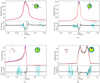 |
Fig. 7 HM and CC microlensing light curves of limb-darkened, blended, and spotted source stars are plotted in a similar way as in Figs. 5 and 6. In these plots, the brightness profiles over the source disks (by considering LD and stellar spots) and the lens trajectory (solid black lines) are shown in the right-hand inside parts. The chromatic perturbations in the V -I and B-R stellar colors by considering only LD, BL effects (solid) and LD, BL as well as stellar spots (dashed) are shown in the residual parts with black and gray curves. The parameters of the light curves are reported in Table 5. |
6 Gravity darkening
Early-type stars such as Be-stars usually rotate very fast and therefore have elliptical shapes. As a result, their surface brightness is not uniform and it increases from the stellar equator toward the poles via the so-called gravity-darkening (GD) effect (see, e.g., Lebovitz 1967; Maeder & Peytremann 1970).
Gravitational microlensing of elliptical source stars have been the subject of a number of works. The first semi-analytical formalism for deriving the magnification factor of elliptical source stars was offered by Heyrovský & Loeb (1997). The effect of ellipticity of the source stars in binary microlensing light curves and close to the caustic fold was also investigated by Gaudi & Haiman (2004); Alexandrov et al. (2018). The GD effect and elliptical shapes of early-type stars change the polarization curves of HM microlensing events and break its symmetry with respect to the time of the closest approach (Sajadian 2016).
The GD effect causes temperature variations over the source disk, such that the stellar temperature is highest at the poles and decreases toward the stellar equator. The temperature variations over the source surface depend on the effective surface gravity which is given by:
![\begin{eqnarray*}\bf{g}_{\textrm{eff}}(\omega, \theta_{\ast}) &\,{=}\,& \Big[-\frac{GM_{\ast}}{R_{\ast}^{2}(\theta_{\ast})} + \omega^{2} R_{\ast}(\theta_{\ast}) \sin^{2} \theta_{\ast}\Big]\bf{e}_{r} \nonumber\\&&+\Big[\omega^{2} R_{\ast}(\theta_{\ast}) \sin \theta_{\ast} \cos \theta_{\ast} \Big] \bf{e}_{\theta},\end{eqnarray*}](/articles/aa/full_html/2022/01/aa41623-21/aa41623-21-eq36.png) (18)
(18)
In this relation, M* is the mass of the source star, ω is the stellar angular velocity around its polar axis, and θ* is the polar angle in the stellar coordinate system. Also, er and eθ are the radial and polar unit vectors in the stellar coordinate system; R* is the stellar radius which for an ellipse depends on the polar angle θ* in the following way (Maeder & Meynet 2012):
![\begin{eqnarray*}R_{\ast}(\theta_{\ast})\,{=}\,\frac{3 R_{\textrm{p}}}{\Omega~\sin \theta_{\ast}} \cos \Big[\frac{\pi + \cos^{-1} (\Omega~\sin \theta_{\ast})}{3}\Big],\end{eqnarray*}](/articles/aa/full_html/2022/01/aa41623-21/aa41623-21-eq37.png) (19)
(19)
where, Rp is the stellar radius at its poles. Ω = ω∕ωc is the stellar angular velocity normalized to the critical (or break up) velocity, which is 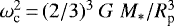 , namely, the velocity at which the gravitational force at the stellar equator equals the centrifugal force.
The effective temperature of an elliptical source star which rotates around its polar axis depends on θ* and can be given as (see, e.g., von Zeipel 1924; Chandrasekhar 1933):
![\begin{eqnarray*}T(\omega,\theta_{\ast})\,{=}\,T_{\textrm{pole}}\Big[~\frac{g_{\textrm{eff}}(\omega,\theta_{\ast})}{G~M_{\ast}/R_{\textrm{p}}^{2}} ~ \Big]^{1/4},\end{eqnarray*}](/articles/aa/full_html/2022/01/aa41623-21/aa41623-21-eq39.png) (20)
(20)
where geff(ω, θ*) is the valueof the effective gravity vector given by Eq. (18); Tpole is the surface temperature at the stellar poles.
In order to model an elliptical source star in the observer’s coordinate system, we use a inclination angle, i, which is the angle between the sky plane and the stellar polar axis. By rotating the source star around x* −axis (which is horizontal and toward right) by the angle − i, we can convert the stellar coordinate system to the observer one and project the source star onto the plane of the sky. The projection process changes the source shape and its eccentricity which can be given by:
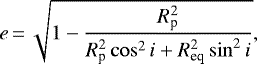 (21)
(21)
where the source radius Req at the equator in the stellar coordinate system is given by Eq. (19) when setting θ* = 90°, such that:
![\begin{eqnarray*}R_{\textrm{eq}}\,{=}\,\frac{3R_{\textrm{p}}}{\Omega} \cos \big[\frac{\pi+ \cos^{-1}\Omega}{3} \big].\\[-13pt] \nonumber\end{eqnarray*}](/articles/aa/full_html/2022/01/aa41623-21/aa41623-21-eq41.png) (22)
(22)
In the observer’s coordinate system, the stellar pole is on the vertical axis on the sky plane and at the position Rp cosi with respect to the source center. If i = 0, the observerwill see both stellar poles.
After simulating an early-type source star, we turn on the lensing effect. For evaluating the magnification factor, we integrate the stellar intensity over the projected source surface. The intensity of each element of the source surface depends on its temperature and is determined by the corresponding Planck function. We simulate a large ensemble of HM microlensing events of elliptical source stars by considering the BL and GD effects. In this regard, we chose the inclination angle and the normalized angular velocity uniformly from the following ranges: i ∈ [0, 90] deg and Ω ∈ [0.2, 0.9]. The stellar temperature at its poles Tpole is calculated according to its mass and using the Besançon model (Robin et al. 2003, 2012).
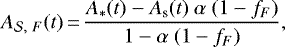
Four examples of these light curves are shown in Fig. 8. The brightness profile of the source star projected on the sky plane and the lens trajectory (solid black lines) are shown in the insets of each light curve panel. The parameters of these light curves are mentioned in Table 6. Some key points are given in the following.
- (i)
If the lens is passing over (or close to) the projected position of the stellar poles, the magnification in the U, B-bands enhances, whereas if the lens is crossing the stellar equator the magnification factor increases in longer wavelengths, for instance, the R, I-bands. As a result, the chromatic perturbations are most often greater in B-R than in V -I (e.g., Figs. 8a,b). This point can be inferred from two the rows (with the label GD) of Table 2.
- (ii)
The chromatic perturbations for these hot stars are asymmetric in time and include consecutive negative-positive deviations, unless either the lens trajectory is parallel with the stellar equator or i = 90°.
- (iii)
Unlike the chromatic perturbations due to the LD effect, the maximum threshold of the GD-induced perturbations does not take place at the time of the closest approach (unless i ~ 90 deg). Their maxima occur when the lens is passing over (or close to) the stellar pole and its equator.
- (iv)
According to the simulation, the amplitude in the chromatic perturbations are ΔCV I, max ~ 0.01, 0.03, 0.06 mag for stars with Ω ≃ 0.5, 0.8, 0.9, respectively. The perturbations will be best observable when the lens is passing very close to the stellar poles. One example light curve is shown in Fig. 8b.
- (v)
We note that the elliptical shape of the source star does not change its color while lensing and the gravity darkening effect does change it.
- (vi)
If the lens does not cross the source surface, the amplitude of the chromatic perturbation is very small and less than 0.02 mag. However, the amplitude depends on Ω.
- (vii)
For such early-type stars as source stars (which are intrinsically bright), the blending effect is very small.
By applying Δχ2 > 100, 200 as detectability criteria (with low and high sensitivities), we conclude that the resulting chromatic perturbations are detectable by the LI camera at the Danish telescope in 62, 54% of HM microlensing events of early-type source stars (with Ω ∈ [0.2, 0.9]). The main reason for such high detection efficiencies is the intrinsic brightness of early-type stars (see Table 6). During CC features, this probability is 41–48%. In these events, the chromatic signatures can reach to 0.4, 0.6 mag for stars with Ω ≃0.7, 0.9. On average, the maximum chromatic deviation in B-R is 0.02–0.03 mag. Measuring chromatic perturbations while lensing will give us some information about the projected location of stellar pole on the sky. However, there is a degeneracy between parameters, because their number is larger than the number of observable quantities.
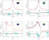 |
Fig. 8 Similar to Figs. 5–7, but for early-type source stars by considering the GD and BL effects. The parameters of the light curves are given in Table 6. The right-hand insets (colored schemes) represent brightness profiles over gravity-darkened source disks and the projected lens trajectory (black lines). In the residual parts, the perturbations in stellar colors due to the GD and BL effects are shown by dashed curves. The corresponding BL-induced chromatic perturbations are represented by solid curves. |
7 Summary and conclusions
The bending angle of light in a gravitational field does not depend on the wavelength of the light. If the brightness of the source star in a microlensing event is homogeneous over the surface and there is no blending effect, then the observed color of the source will not change during the lensing. One way to distinguish microlensing events from other astrophysical phenomena in which the stellar brightness changes with time is therefore to check whether the stellar color changes with the changing brightness. However, if the color of the source star is not identical all over its surface or the blending effect is considerable, the different magnification factors in different filters will cause the color of the lensing event to change as function of time. These chromatic variations are most pronounced in HM and binary CC microlensing events.
The surface brightness of the source stars may vary due to (i) the limb-darkening, (ii) close-in giant planet companions, (iii) stellar spots and (iv) gravity-darkening. In all of these situations, the stellar color changes as function of time during the lensing. Additionally, the BL effect in microlensing events leads to chromatic perturbations during lensing. In fact, the blending parameter depends on the adopted filter. In this work, we evaluated the resulting perturbations in the V -I and B-R stellar colors in HM and CC events by considering the aforementioned effects. Since HM and CC microlensing events are followed by use of the dual-color LI camera on Danish 1.54 m telescope by our team, we have in the present work estimated the probability of detecting these perturbations in the V -I stellar color by use of this camera, which are summarized in Table 2.
The importance of studying the chromatic perturbations are twofold: (i) since the perturbations are time-dependent, then different sets of data points taken for a microlensing event in different filters (often by different telescopes) cannot be converted to the same filter in order to determine a best-fitting model. The relations for converting magnitudes in different filters are applicable only when the lens-source distance is sufficiently large, such than the source radius does not give rise to a finite-source effect (i.e., near the baseline of the event). Ignoring these perturbations while modeling HM or CC microlensing events creates extra noise in the converted data points (especially the data around the magnification peaks). (ii) Dual-color instruments can potentially measure these chromatic perturbations and allow determination of the variation in the surface brightness and color of the source stars. That is another channel for probing the surface of Galactic bulge stars.
The BL effect in microlensing events makes chromatic variations for the source stars. The movement of source stars in the color-color diagram (due to the BL-induced chromatic perturbations) helps to determine the stellar types (Tsapras et al. 2019). The BL-induced chromatic perturbation enhances by increasing the magnification peak. Its increasing slope tends to zero for the magnification factor larger than 40. The time scale of these chromatic perturbations is of order tE (the time scale of the lensing effect). For transit microlensing events (with the considerable finite-source effect), the magnification factor remains almost constant while passing the source surface. Hence, in these events and around their peaks, the BL-induced chromatic perturbations are almost constant and can be subtracted from the chromatic variation curves.
By simulating HM microlensing events of source stars and including a LD effect, we concluded that for transit microlensing events, the light curves are more flattened in longer wavelength (lower peak and larger width) than at shorter wavelengths. In these events, the chromatic perturbations are maximized at the time of the closest approach and can even reach 0.04 mag (measurableby our LI camera). For non-transit microlensing events, the peaks of light curves are maximized in the I-band and the maximum chromatic perturbations reach 0.01 mag. DuringCC and when the source edge is passing from the caustic line and the source center is out of the caustic, these chromatic signals are higher, reaching 0.07 mag. We note that the level of chromatic perturbations due to LD effects in the B-R color is higher than in V -I. The probabilities of detecting LD and BD-induced perturbations in V -I by our LI camera are 50–60, 20–30% in HM and CC events, respectively. We considered Δχ2 > 200, 100 as the detectability threshold.
Close-in giant planets orbiting the source stars with an inclination angle ~ 90 deg (i.e., edge-on orbits) transit their host stars and make periodic changes in their brightness and color distribution over the surface. We studied whether this kind of variation in the stellar brightness can make significant chromatic perturbations during lensing. The probability for detecting planet-induced chromatic perturbations for face-on planetary orbits is low, because it would require that the lensing star passes very close to (or over) the planet surface, which is small. For edge-on orbits the probability is higher, because it is the change in color of the source star (where the planet transits) that is amplified by the lens, and causes the achromatic effects, and reveals the planet. By including both the LD, BL and CGPs orbiting the source stars, we concluded that the probabilities for detecting the chromatic perturbation in HM or CC events are 53–64, 23–32%, respectively. We note that CGPs improve the detection probability of chromatic perturbations by ~ 2%.
By adding the stellar spots for limb-darkened and blended source stars, these probabilities increase to 51–63, 27–36% in HM and CC events, respectively. In these events, if the lens transits the stellar spot, an extra bump appears in the V -I light curve of the source star which alters the stellar color up to 0.05 mag. The spot-induced perturbations in the V -I color are higher than in B-R. The SS-induced chromatic perturbations can be degenerate with those made by transiting CGPs.
Early-type source stars do not have constant surface brightness because of the gravity-darkening effect which comes from the elliptical shape of these stars. If the lens transits the source surface and passes close to (or over) the stellar poles, the chromatic perturbation maximizes and reaches 0.01, 0.03, 0.06 mag for stars with Ω ~ 0.5, 0.8, 0.9, respectively. Our LI camera can potentially discover these perturbations with a probability of 54–62, 41–48% when it is observing HM and CC events.
Acknowledgements
We acknowledge support from the European Union H2020-MSCA-ITN-2019 under Grant no. 860470 (CHAMELEON) and from the Novo Nordisk Foundation Interdisciplinary Synergy Program grant no. NNF19OC0057374. S.S. thanks the Department of Physics, Chungbuk National University and especially C. Han for hospitality. We thank M. Hundertmark, J. Scottfelt and D. Bramich for consultations. We appreciate the referee for the helpful comments and good suggestions.
Appendix A Photometric uncertainties of data taken by the Danish telescope
The error bars of data taken by LI camera on the Danish telescope in the Johnson R-band were well studied in Skottfelt et al. (2015). The authors have measured the root mean square (RMS) magnitude deviations, δR, versus the stellar apparent magnitudes in the R-band. The data-reduction of their images have been done using DanIDL4 pipeline (Bramich 2008; Bramich et al. 2013). We use their results to determine the error bars of synthetic data points taken by LI camera in our simulation. We show their measurements in Figure A.1 and fit a hybrid linear curve to the data. The equation of the fitted hybrid function is:
![\begin{eqnarray*}&&\hskip-7pt \log_{10}[\delta_{R}]=\nonumber \\&&\begin{cases}0.256({\pm}0.005)~m_{R} -6.282({\pm}0.09) & m_{R} \leq 18.5\\0.333({\pm}0.004)~m_{R} -7.707({\pm}0.09) & m_{R}>18.5.\end{cases}\end{eqnarray*}](/articles/aa/full_html/2022/01/aa41623-21/aa41623-21-eq42.png) (A.1)
(A.1)
In order to estimate error bars in standard Johnson filters V and I for synthetic data taken by LI, we use two relations between the photometric measurements in R and V, I-bands. These relations are explained in the following.
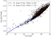 |
Fig. A.1 The scatter plot of RMS magnitude deviation versus mean R- band magnitude as measured by the LI camera on Danish telescope and reported in Skottfelt et al. (2015). The dashed lines represent the best-fitted linear curves to black data points and given by Equations 18. |
The best-fitted parameters of linear relation between mV + mI versus mR for different values of the stellar age and metalicity. A complete electronic version of this table is available at the CDS.
The stellar magnitude in the R-band is approximately the average of the corresponding magnitudes in the V and I-bands. However, the stellar age and metalicity change the stellar spectra somewhat. In order to find an accurate relation between the stellar magnitudes for any given values of stellar age and matelicity, we use the Dartmouth stellar Isochrones 5 (Dotter et al. 2008). For any given values of stellar age and matellicity and for different stars with different initial mass, we fit a linear relation between the R-band and V + I-band magnitudes, as mV + mI = a mR + b. In Table A.1, the slope and offset of these linear relations for different stellar age and metalicity values are given.
Another relation between these error bars is necessary to determine their contributions. In our simulation and for each given value of magnification factor, AF(t), we can determine the ratio of signal to noise ratio (S/N) in these two filters as follows:
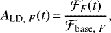
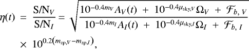 (A.3)
(A.3)
where 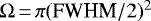 is the area of the stellar PSF. FWHM is the Full Width at Half Maximum of the stellar brightness profile. For LI camera on the Danish telescope FWHM ≃ 0.48, 0.46 arcs in V and I-bands (Skottfelt et al. 2015). The sky brightness at the La Silla observatory was reported as μsky = 21.75, 19.48 mag. arcs−2 in V and I-bands, respectively (Mattila et al. 1996). We do not need to include the exposure time in this ratio, because LI camera has the same exposure times for images taken in these two filters. This ratio, η(t), gives another relation between the photometric error bars in V and I-bands as follows:
 (A.4)
(A.4)
Using the relations A.2 and A.4, we determine photometric error bars for each couple of data points taken by LI camera on the Danish telescope in V and I-bands. We note that a similar method was used to estimate the error bars of data points taken by the Danish telescope in Evans et al. (2018, 2016).
References
- Alexandrov, A., Zhdanov, V., & Kuybarov, A. 2018, Bull. Taras Shevchenko National Univ. Kyiv Astron., 57, 10 [CrossRef] [Google Scholar]
- Bagheri, F., Sajadian, S., & Rahvar, S. 2019, MNRAS, 490, 1581 [NASA ADS] [CrossRef] [Google Scholar]
- Beaulieu, J. P., Bennett, D. P., Fouqué, P., et al. 2006, Nature, 439, 437 [NASA ADS] [CrossRef] [Google Scholar]
- Borucki, W. J., Koch, D., Basri, G., et al. 2010, Science, 327, 977 [Google Scholar]
- Bozza, V. 2010, MNRAS, 408, 2188 [NASA ADS] [CrossRef] [Google Scholar]
- Bozza, V., Bachelet, E., Bartolić, F., et al. 2018, MNRAS, 479, 5157 [Google Scholar]
- Bramich, D. M. 2008, MNRAS, 386, L77 [NASA ADS] [CrossRef] [Google Scholar]
- Bramich, D. M., Horne, K., Albrow, M. D., et al. 2013, MNRAS, 428, 2275 [NASA ADS] [CrossRef] [Google Scholar]
- Castelli, F., & Kurucz, R. L. 2003, IAU Symp., 210, A20 [Google Scholar]
- Chandrasekhar, S. 1933, MNRAS, 93, 462 [NASA ADS] [Google Scholar]
- Chandrasekhar, S. 1960, Radiative Transfer (New York: Dover Publications) [Google Scholar]
- Chang, K., & Refsdal, S. 1979, Nature, 282, 561 [Google Scholar]
- Code, A. D. 1950, ApJ, 112, 22 [NASA ADS] [CrossRef] [Google Scholar]
- Di Stefano, R., & Esin, A. A. 1995, ApJ, 448, L1 [NASA ADS] [CrossRef] [Google Scholar]
- Dominik, M., Jorgensen, U. G., Horne, K., et al. 2008, ArXiv e-prints [arXiv:0808.0004] [Google Scholar]
- Dominik, M., Jørgensen, U. G., Rattenbury, N. J., et al. 2010, Astron. Nachr., 331, 671 [NASA ADS] [CrossRef] [Google Scholar]
- Dotter, A., Chaboyer, B., Jevremović, D., et al. 2008, ApJS, 178, 89 [Google Scholar]
- Einstein, A. 1936, Science, 84, 506 [NASA ADS] [CrossRef] [Google Scholar]
- Evans, D. F., Southworth, J., Maxted, P. F. L., et al. 2016, A&A, 589, A58 [NASA ADS] [CrossRef] [EDP Sciences] [Google Scholar]
- Evans, D. F., Southworth, J., Smalley, B., et al. 2018, A&A, 610, A20 [NASA ADS] [CrossRef] [EDP Sciences] [Google Scholar]
- Gaudi, B. S. 2012, ARA&A, 50, 411 [Google Scholar]
- Gaudi, B. S., & Haiman, Z. 2004, ArXiv e-prints [arXiv:astro-ph/0401035] [Google Scholar]
- Giordano, M., Nucita, A. A., De Paolis, F., & Ingrosso, G. 2015, MNRAS, 453, 2017 [NASA ADS] [CrossRef] [Google Scholar]
- Gould, A., & Loeb, A. 1992, ApJ, 396, 104 [Google Scholar]
- Graff, D. S., & Gaudi, B. S. 2000, ApJ, 538, L133 [NASA ADS] [CrossRef] [Google Scholar]
- Gustafsson, B., Edvardsson, B., Eriksson, K., et al. 2008, A&A, 486, 951 [NASA ADS] [CrossRef] [EDP Sciences] [Google Scholar]
- Han, C., & Park, S.-H. 2001, MNRAS, 320, 41 [NASA ADS] [CrossRef] [Google Scholar]
- Han, C., Park,S.-H., & Jeong, J.-H. 2000a, MNRAS, 316, 97 [NASA ADS] [CrossRef] [Google Scholar]
- Han, C., Park,S.-H., Kim, H.-I., & Chang, K. 2000b, MNRAS, 316, 665 [NASA ADS] [CrossRef] [Google Scholar]
- Han, C., Calchi Novati, S., Udalski, A., et al. 2018, ApJ, 859, 82 [NASA ADS] [CrossRef] [Google Scholar]
- Harpsøe, K. B. W., Jørgensen, U. G., Andersen, M. I., & Grundahl, F. 2012, A&A, 542, A23 [NASA ADS] [CrossRef] [EDP Sciences] [Google Scholar]
- Harrington, J. P. 1970, Ap&SS, 8, 227 [NASA ADS] [CrossRef] [Google Scholar]
- Harrington, J. P. 2015, in IAU Symposium, 305, Polarimetry, eds. K. N. Nagendra, S. Bagnulo, R. Centeno, & M. Jesús Martínez González, 395–400 [NASA ADS] [Google Scholar]
- Harrington, J. P. 2017, Nat. Astron., 1, 657 [NASA ADS] [CrossRef] [Google Scholar]
- Hendry, M. A., Bryce, H. M., & Valls-Gabaud, D. 2002, MNRAS, 335, 539 [NASA ADS] [CrossRef] [Google Scholar]
- Heyrovský, D., & Loeb, A. 1997, ApJ, 490, 38 [CrossRef] [Google Scholar]
- Heyrovský, D., & Sasselov, D. 2000, ApJ, 529, 69 [CrossRef] [Google Scholar]
- Hirao, Y., Bennett, D. P., Ryu, Y.-H., et al. 2020, AJ, 160, 74 [NASA ADS] [CrossRef] [Google Scholar]
- Hwang, K.-H.,& Han, C. 2010, ApJ, 709, 327 [NASA ADS] [CrossRef] [Google Scholar]
- Kondo, I., Yee, J. C., Bennett, D. P., et al. 2021, AJ, 162, 77 [NASA ADS] [CrossRef] [Google Scholar]
- Kurucz, R. 1993, ATLAS9 Stellar Atmosphere Programs and 2 km/s grid, Kurucz CD-ROM No. 13. (Cambridge: Cambridge University Press), 13 [Google Scholar]
- Lanz, T., & Hubeny, I. 2003, ApJS, 146, 417 [NASA ADS] [CrossRef] [Google Scholar]
- Lanz, T., & Hubeny, I. 2007, ApJS, 169, 83 [CrossRef] [Google Scholar]
- Lebovitz, N. R. 1967, ARA&A, 5, 465 [NASA ADS] [CrossRef] [Google Scholar]
- Li, S. S., Zang, W., Udalski, A., et al. 2019, MNRAS, 488, 3308 [NASA ADS] [CrossRef] [Google Scholar]
- Liebes, S. 1964, Phys. Rev., 133, B835 [NASA ADS] [CrossRef] [Google Scholar]
- Maeder, A., & Meynet, G. 2012, Rev. Mod. Phys., 84, 25 [Google Scholar]
- Maeder, A., & Peytremann, E. 1970, A&A, 7, 120 [NASA ADS] [Google Scholar]
- Mao, S., & Paczynski, B. 1991, ApJ, 374, L37 [NASA ADS] [CrossRef] [Google Scholar]
- Mattila, K., Vaeisaenen, P., & Appen-Schnur, G. F. O. V. 1996, A&AS, 119, 153 [NASA ADS] [CrossRef] [EDP Sciences] [Google Scholar]
- Moniez, M., Sajadian, S., Karami, M., Rahvar, S., & Ansari, R. 2017, A&A, 604, A124 [NASA ADS] [CrossRef] [EDP Sciences] [Google Scholar]
- Mróz, P., Udalski, A., Skowron, J., et al. 2017, Nature, 548, 183 [Google Scholar]
- Mróz, P., Udalski, A., Skowron, J., et al. 2019, ApJS, 244, 29 [Google Scholar]
- Mróz, P., Poleski, R., Han, C., et al. 2020, AJ, 159, 262 [CrossRef] [Google Scholar]
- Paczynski, B. 1986, ApJ, 304, 1 [NASA ADS] [CrossRef] [Google Scholar]
- Paczynski, B., Udalski, A., Szymanski, M., et al. 1999, Acta Astron., 49, 319 [NASA ADS] [Google Scholar]
- Pejcha, O., & Heyrovský, D. 2009, ApJ, 690, 1772 [NASA ADS] [CrossRef] [Google Scholar]
- Rahvar, S., & Dominik, M. 2009, MNRAS, 392, 1193 [CrossRef] [Google Scholar]
- Robin, A. C., Reylé, C., Derrière, S., & Picaud, S. 2003, A&A, 409, 523 [NASA ADS] [CrossRef] [EDP Sciences] [Google Scholar]
- Robin, A. C., Marshall, D. J., Schultheis, M., & Reylé, C. 2012, A&A, 538, A106 [NASA ADS] [CrossRef] [EDP Sciences] [Google Scholar]
- Ryu, Y. H., Yee, J. C., Udalski, A., et al. 2018, AJ, 155, 40 [Google Scholar]
- Sajadian, S. 2015, MNRAS, 452, 2587 [CrossRef] [Google Scholar]
- Sajadian, S. 2016, ApJ, 825, 152 [NASA ADS] [CrossRef] [Google Scholar]
- Sajadian, S. 2021, MNRAS, 506, 3615 [NASA ADS] [CrossRef] [Google Scholar]
- Sajadian, S., & Hundertmark, M. 2017, ApJ, 838, 157 [NASA ADS] [CrossRef] [Google Scholar]
- Sajadian, S., & Ignace, R. 2020a, MNRAS, 494, 1735 [NASA ADS] [CrossRef] [Google Scholar]
- Sajadian, S., & Ignace, R. 2020b, MNRAS, 498, 223 [NASA ADS] [CrossRef] [Google Scholar]
- Sajadian, S., & Poleski, R. 2019, ApJ, 871, 205 [NASA ADS] [CrossRef] [Google Scholar]
- Sajadian, S., & Rahvar, S. 2010, MNRAS, 407, 373 [NASA ADS] [CrossRef] [Google Scholar]
- Sajadian, S., Rahvar, S., Dominik, M., & Hundertmark, M. 2016, MNRAS, 458, 3248 [NASA ADS] [CrossRef] [Google Scholar]
- Sajadian, S., Ignace, R., & Neilson, H. 2021, MNRAS, 507, 5177 [NASA ADS] [CrossRef] [Google Scholar]
- Schneider, P., Ehlers, J., & Falco, E. E. 1992, Gravitational Lenses [Google Scholar]
- Skottfelt, J., Bramich, D. M., Hundertmark, M., et al. 2015, A&A, 574, A54 [NASA ADS] [CrossRef] [EDP Sciences] [Google Scholar]
- Skowron, J., & Gould, A. 2012, ArXiv e-prints [arXiv:1203.1034] [Google Scholar]
- Smith, M. C., Woźniak, P., Mao, S., & Sumi, T. 2007, MNRAS, 380, 805 [NASA ADS] [CrossRef] [Google Scholar]
- Street, R. A., Bachelet, E., Tsapras, Y., et al. 2019, AJ, 157, 215 [NASA ADS] [CrossRef] [Google Scholar]
- Tsapras, Y. 2018, Geosciences, 8, 365 [NASA ADS] [CrossRef] [Google Scholar]
- Tsapras, Y., Street, R. A., Hundertmark, M., et al. 2019, PASP, 131, 124401 [NASA ADS] [CrossRef] [Google Scholar]
- Udalski, A., Ryu, Y. H., Sajadian, S., et al. 2018, Acta Astron., 68, 1 [NASA ADS] [Google Scholar]
- Valls-Gabaud, D. 1998, MNRAS, 294, 747 [CrossRef] [Google Scholar]
- Van Eck, S., Neyskens, P., Jorissen, A., et al. 2017, A&A, 601, A10 [NASA ADS] [CrossRef] [EDP Sciences] [Google Scholar]
- von Zeipel, H. 1924, MNRAS, 84, 665 [NASA ADS] [CrossRef] [Google Scholar]
- Zub, M., Cassan, A., Heyrovský, D., et al. 2011, A&A, 525, A15 [NASA ADS] [CrossRef] [EDP Sciences] [Google Scholar]
For instance, the Danish telescope has densely followed 68 anomalous and highly-magnified microlensing events alarmed by the ARTEMiS system in 2008 with high photometric precisions (Dominik et al. 2010).
All Tables
LI efficiencies for detecting chromatic perturbations in HM single and CC binary microlensing events and the properties of these events.
The best-fitted parameters of linear relation between mV + mI versus mR for different values of the stellar age and metalicity. A complete electronic version of this table is available at the CDS.
All Figures
|
Fig. 1 Variation in the stellar colors V -I (red) and B-R (green) versus the magnification factor due to the BL effect. The adopted blending parameters, given in the figure, are the average of blending parameters for simulated microlensing events toward the Baade’s window, with the coordinate (lG = 1°, bG = − 4°), by excludinghighly blended events with bI < 0.2. |
| In the text | |
|
Fig. 2 HM and CC microlensing light curves of blended source stars in the passband filters UBV RI, are shown by magenta, blue, green, orange, and red colors, respectively. The perturbations in stellar colors V -I and B-R during the lensing effect are shown in the residual parts by solid (black and gray) curves, respectively. The source star parameters are listed in Table 1. The synthetic data points by the LI camera at the Danish telescope in the I-band are shownwith red filled circles. The corresponding data points over the residual parts (related to the V -I color) are plotted by cyan filled points. In the two top panels, each right-hand inset shows the source star (blue circle) and the lenstrajectory (black line) both projected on the lens plane. In the bottom panels, each right-hand inset shows the caustic curve (brown curve) and the source trajectory (black line) projected onto the lens plane. |
| In the text | |
|
Fig. 3 Emergent radiation intensities for four stars with different temperature and the surface gravity values versus μ in the standard filters, UBV RI, as shown with magenta, blue, green, orange, and red curves. |
| In the text | |
|
Fig. 4 LD coefficients, ΓF, in different filters F, ∈ UBV RI (shown with magenta, blue, green, orange and red colors, respectively), for stars with different effective surface temperatures and two values of the surface gravity (given at the top of the plots). |
| In the text | |
|
Fig. 5 HM and CC microlensing light curves of limb-darkened and blended source stars are plotted. Details are similar to those in Fig. 2. The lensing parameters are listed in Table 3. In the residual parts, the perturbations in stellar colors V -I and B-R during the lensing effect due to LD and BL effects are shown by dashed (black and gray) curves, respectively. The corresponding chromatic BL-induced perturbations are shown by solid curves. The right-hand insets (colored schemes) represent brightness profiles over limb-darkened source disks. |
| In the text | |
|
Fig. 6 HM and CC microlensing light curves of limb-darkened and blended source stars are plotted, but we additionally consider a close-in giant planet around each source star. Details are similar to those in Fig. 5. In each panel, the source star (blue circle), its planet (red circle), the planet orbit projected on the sky plane (green curve), and the lens trajectory (black solid line) are shown as insets in the figures. The chromatic perturbations in the V -I and B-R stellar colors by considering only the LD and BL effects (solid) and LD, BL plus a source star planet (dashed) are shown in the residual parts with black and gray curves. Their parameters are given in Table 4. |
| In the text | |
|
Fig. 7 HM and CC microlensing light curves of limb-darkened, blended, and spotted source stars are plotted in a similar way as in Figs. 5 and 6. In these plots, the brightness profiles over the source disks (by considering LD and stellar spots) and the lens trajectory (solid black lines) are shown in the right-hand inside parts. The chromatic perturbations in the V -I and B-R stellar colors by considering only LD, BL effects (solid) and LD, BL as well as stellar spots (dashed) are shown in the residual parts with black and gray curves. The parameters of the light curves are reported in Table 5. |
| In the text | |
|
Fig. 8 Similar to Figs. 5–7, but for early-type source stars by considering the GD and BL effects. The parameters of the light curves are given in Table 6. The right-hand insets (colored schemes) represent brightness profiles over gravity-darkened source disks and the projected lens trajectory (black lines). In the residual parts, the perturbations in stellar colors due to the GD and BL effects are shown by dashed curves. The corresponding BL-induced chromatic perturbations are represented by solid curves. |
| In the text | |
|
Fig. A.1 The scatter plot of RMS magnitude deviation versus mean R- band magnitude as measured by the LI camera on Danish telescope and reported in Skottfelt et al. (2015). The dashed lines represent the best-fitted linear curves to black data points and given by Equations 18. |
| In the text | |
Current usage metrics show cumulative count of Article Views (full-text article views including HTML views, PDF and ePub downloads, according to the available data) and Abstracts Views on Vision4Press platform.
Data correspond to usage on the plateform after 2015. The current usage metrics is available 48-96 hours after online publication and is updated daily on week days.
Initial download of the metrics may take a while.