| Issue |
A&A
Volume 655, November 2021
|
|
|---|---|---|
| Article Number | A54 | |
| Number of page(s) | 28 | |
| Section | Cosmology (including clusters of galaxies) | |
| DOI | https://doi.org/10.1051/0004-6361/202040140 | |
| Published online | 19 November 2021 | |
Theoretical and numerical perspectives on cosmic distance averages
1
Aix Marseille Univ., CNRS, CNES, LAM, Marseille, France
e-mail: This email address is being protected from spambots. You need JavaScript enabled to view it.
2
Instituto de Física Teórica UAM-CSIC, Universidad Autónoma de Madrid, Cantoblanco, 28049 Madrid, Spain
e-mail: This email address is being protected from spambots. You need JavaScript enabled to view it.
Received:
16
December
2020
Accepted:
15
August
2021
Abstract
The interpretation of cosmological observations relies on a notion of an average Universe, which is usually considered as the homogeneous and isotropic Friedmann-Lemaître-Robertson-Walker (FLRW) model. However, inhomogeneities may statistically bias the observational averages with respect to FLRW, notably for distance measurements, due to a number of effects such as gravitational lensing and redshift perturbations. In this article, we review the main known theoretical results on average distance measures in cosmology, based on second-order perturbation theory, and we fill in some of their gaps. We then comprehensively test these theoretical predictions against ray tracing in a high-resolution dark-matter N-body simulation. This method allows us to describe the effect of small-scale inhomogeneities deep into the non-linear regime of structure formation on light propagation up to z = 10. We find that numerical results are in remarkably good agreement with theoretical predictions in the limit of super-sample variance. No unexpectedly large bias originates from very small scales, whose effect is fully encoded in the non-linear power spectrum. Specifically, the directional average of the inverse amplification and the source-averaged amplification are compatible with unity; the change in area of surfaces of constant cosmic time is compatible with zero; the biases on other distance measures, which can reach slightly less than 1% at high redshift, are well understood. As a side product, we also confront the predictions of the recent finite-beam formalism with numerical data and find excellent agreement.
Key words: large-scale structure of Universe / distance scale / cosmology: theory / methods: numerical
© M.-A. Breton and P. Fleury 2021
 Open Access article, published by EDP Sciences, under the terms of the Creative Commons Attribution License (https://creativecommons.org/licenses/by/4.0), which permits unrestricted use, distribution, and reproduction in any medium, provided the original work is properly cited.
1. Introduction
On very large scales, our Universe seems to be well described by a spatially homogeneous and isotropic Friedmann-Lemaître-Robertson-Walker (FLRW) model (Green & Wald 2014). This model allows us to predict the dynamics of cosmic expansion as a function of the Universe’s content, and of the laws of gravitation. Furthermore, the FLRW model constitutes a rather efficient framework to interpret the observation of remote light sources; in particular, it provides the relation between their redshift z and their angular or luminosity distance D.
The distance-redshift relation D(z) is prominent in cosmology, as it is involved in the interpretation of various observables. Its first derivative today defines the Hubble-Lemaître constant, dD/dz|0 = c/H0, whose exact value is still subject to a lively debate (Planck Collaboration VI 2020; Riess et al. 2019; Wong et al. 2019; Freedman et al. 2019). More generally, D(z) constitutes the essence of the Hubble diagram of type-Ia supernovae (SNe, Scolnic et al. 2018; Abbott et al. 2019), which historically revealed the acceleration of cosmic expansion (Perlmutter & Aldering 1998; Riess et al. 1998), as well as the Hubble diagram of gravitational-wave standard sirens in the near future (Holz & Hughes 2005; Caprini & Tamanini 2016). The D(z) relation is also essential in the analysis of the anisotropies of the cosmic microwave background (CMB, Planck Collaboration VI 2020), or in the baryon-acoustic oscillation signal observed in galaxy, Lyman-α or quasar surveys (Alam et al. 2021), because it converts the observed angular size of the sound horizon θ* into a physical distance rs = D(z*)θ* that may be predicted by theory.
In the actual inhomogeneous Universe, however, the D(z) relation is affected by various effects, such as gravitational lensing (Schneider et al. 1992) which tends to focus and distort light beams, thereby changing the apparent size and brightness of light sources; it is also affected by the peculiar velocities of the sources and the observer, which correct the observed redshift via the Doppler effect (Hui & Greene 2006; Davis et al. 2011). Such effects make D(z) line-of-sight dependent, but it is generally assumed that the FLRW prediction is recovered on average.
The fundamental question of whether the average D(z) is the same as the D(z) of the average Universe goes back more than 50 years, when Zel’dovich (1964) and Feynman (in a colloquium given at Caltech the same year)1 suggested the following: if the Universe is lumpy, then a typical light beam should mostly propagate through under-dense regions, and thereby be de-focussed with respect to FLRW; this should imply that D(z) is actually biased up. Many developments and counter-arguments followed from that seminal idea; we refer the interested reader to the introduction of Kaiser & Peacock (2016, hereafter KP16) and the comprehensive review by Helbig (2020) for details.
In that debate, a significant step was made by Weinberg (1976), who showed that in a Universe sparsely filled with point masses, the average flux ∝⟨1/D2(z)⟩ is the same as if the matter in those lenses were homogeneously distributed in space. Importantly, Weinberg’s calculation was made at first order in the small projected density of the lenses2. As such, it also implies that ⟨D(z)⟩ is unaffected by inhomogeneities at that order, because the difference between ⟨1/D2⟩ and 1/⟨D⟩2 only appears at second order. Weinberg nevertheless conjectured, on the basis of flux conservation, that the invariance of ⟨1/D2(z)⟩ may be exact and hold for any matter distribution. As noted by Ellis et al. (1998), this general flux-conservation argument is, in fact, incomplete because it implicitly assumes that the area of surfaces of constant redshift are unaffected by inhomogeneities, which is a mere reformulation of the whole problem.
For a long period of time, all this discussion remained mostly centred on the observation of individual sources, with the aim of predicting possible biases on the Hubble diagram; it became a somewhat marginal topic from the end of the 1980s, presumably because the precision of cosmological measurements was not sufficient to be sensitive to the expected biases on ⟨D(z)⟩. Interest in that matter was nevertheless revived by Clarkson et al. (2014), who made the rather surprising claim that lensing affects the distance to the last-scattering surface (LSS) at percent level, which would be dramatic for the standard interpretation of the CMB. This claim was then retracted by (almost) the same team in Bonvin et al. (2015a), who with KP16 clarified that: (i) the average distance to the LSS is not relevant to the standard CMB analysis; and (ii) one must distinguish between the concepts of directional averaging, source-averaging, or ensemble-averaging, which may yield different results (Bonvin et al. 2015b). Such considerations on cosmological averages were actually elaborating on an earlier work by Kibble & Lieu (2005).
In the end, for the CMB just as for the Hubble diagram, the whole problem boils down to the validity of Weinberg’s conjecture which states that the area of LSS, A*, or the area of constant-redshift surfaces, A(z), are not significantly affected by inhomogeneities. KP16 undertook the difficult task to explicitly check this conjecture in the framework of cosmological perturbations at second order. With a rather intuitive approach, KP16 identified several key effects such as the shortening of the radius reached by rays due to their deflection, or the increase in A* due to its wrinkles, and eventually reached the conclusion that A* cannot be biased by more than a part in a million. They identified that the relevant structures responsible for such a bias are rather large in size, of the order of 50 h−1 Mpc.
Most of the theoretical work depicted above was done using cosmological perturbation theory on an FLRW background (see also Sasaki 1987; Bonvin et al. 2006; Ben-Dayan et al. 2012; Umeh et al. 2014; Yoo & Scaccabarozzi 2016). However, this theoretical framework is not guaranteed to provide a good representation of the Universe, as it does not access the highly non-linear regime of structure formation. That is why one may prefer to rely on numerical simulations and ray-tracing methods, in order to accurately describe the propagation of light in a realistic picture of the cosmos.
As a first step, a significant research endeavour was dedicated to ray tracing and distance measurements in cosmological toy-models, such as Swiss-cheese models (Brouzakis et al. 2007, 2008; Marra et al. 2008; Biswas & Notari 2008; Vanderveld et al. 2008; Valkenburg 2009; Clifton & Zuntz 2009; Bolejko 2009, 2011; Bolejko & Célérier 2010; Szybka 2011; Flanagan et al. 2013; Fleury et al. 2013; Fleury 2014; Troxel et al. 2014; Peel et al. 2014; Lavinto & Rasanen 2015; Koksbang 2017, 2019a,b, 2020a), plane-parallel Universes (Di Dio et al. 2012), or lattice models (Clifton & Ferreira 2009a,b, 2011; Clifton et al. 2012; Liu 2015; Bruneton & Larena 2013; Bentivegna et al. 2017; Sanghai et al. 2017; Koksbang 2020b). These works generally agreed with the relevant theoretical predictions. Using N-body simulations, Odderskov et al. (2016) showed that at low redshift (z < 0.1), the averaged luminosity distance is very close from its value in an FLRW background. Within the field of numerical relativity, Giblin et al. (2016) showed that ⟨log D⟩ (or averaged magnitude) was not affected by inhmogeneities, at least until z = 1.5. However, both studies used simulations with rather low resolution, which might be subject to large variance and therefore could not highlight second-order effects. More recently, Adamek et al. (2019) used the general-relativistic simulation gevolution (Adamek et al. 2016), and accurate ray tracing to find null geodesics between sources and observer and produce realistic halo catalogues. They found that when averaging over sources, ⟨1/D2(z)⟩ is very close to its value from a homogeneous Universe, until z = 3, thereby confirming Weinberg’s conjecture, while ⟨D(z)⟩ is slightly biased as expected. Albeit a high-resolution, gevolution remains a particle-mesh code without adaptive-mesh refinement, which thus cannot access very small scales.
In the present article, we propose a short theoretical review, and a detailed numerical study of the bias in the distance-redshift relation with respect to the standard FLRW prediction. The theory part builds upon KP16 and fills minor conceptual gaps therein. In the main, numerical, part we use a high-resolution N-body simulation part of the ‘Raygal’ suite and propagate photons on null geodesics to infer distance measures, accounting for gravitational lensing and redshift perturbations. Taking advantage of very large statistics and wide redshift range (up to z = 10), we investigate the different averaging procedures and study the statistics to the related observables. Furthermore, we numerically estimate the area bias depending on the choice of light-cone slicing.
The article is organised as follows. Section 2 presents the formalism for light propagation and the bias on statistical quantities with respect to the homogeneous case, depending on the averaging procedure; we connect these notions to the area of slices of the light cone. The numerical simulation, ray-tracing methods, and analysis techniques, are presented in Sect. 3, while the results are exposed in Sect. 4. We conclude in Sect. 5.
Notation and conventions. Greek indices (μ, ν, …) run from 0 to 3 and Latin indices (i, j, …) from 1 to 3. Bold symbols denote Euclidean two-dimensional or three-dimensional vectors, and matrices. Over-barred symbols denote quantities computed in a homogeneous-isotropic FLRW model. We adopt units in which the speed of light is unity, c = 1.
2. Theory
This section gathers a number of already-established theoretical results about light propagation in the inhomogeneous Universe, as well as a few novel elements, such as the distinction between lensing magnification and amplification and its interpretation. We shall focus on the statistical averages of distance measures, and how they relate to the area of light-cone slices.
2.1. Light propagation in a perturbed FLRW Universe
We consider a cosmological space-time described by a spatially flat FLRW model with scalar perturbations. The associated line element reads, in the Newtonian gauge
![Mathematical equation: $$ \begin{aligned} \mathrm{d} s^2 = a^2(\eta )\left[-(1+2\phi )\mathrm{d} \eta ^2 + (1-2\phi )\mathrm{d} \boldsymbol{x}^2\right], \end{aligned} $$](/articles/aa/full_html/2021/11/aa40140-20/aa40140-20-eq1.gif) (1)
(1)
where η denotes the conformal time (hereafter simply referred to as time), xi are comoving coordinates, a(η) the scale factor describing cosmic expansion, and ϕ the Bardeen potential (Bardeen 1980) caused by inhomogeneities in the matter density field. We assume that anisotropic stress is negligible so that this potential is unique. Except in the vicinity of compact objects, ϕ ≪ 1 can be treated as a perturbation. The time at the observation event (here and now) is denoted η0, where the scale factor is conventionally set to unity, a0 = a(η0) = 1.
Light propagates along null geodesics of the space-time geometry. In the absence of perturbations (that is, for ϕ = 0), such geodesics are straight lines in comoving coordinates, travelled with unit coordinate speed. In the presence of perturbations, light rays are bent and the coordinate speed of light effectively varies (Schneider et al. 1992). These effects are encoded in the null geodesic equation kν∇νkμ = 0, with kμ ≡ dxμ/dλ and λ denotes a past-oriented affine parameter for the light ray. The temporal and spatial components of the geodesic equation read
 (2)
(2)
 (3)
(3)
where ℋ ≡ a−1da/dη is the conformal expansion rate. Equation (2) rules the evolution of light’s frequency in the cosmic frame; combined with the latter, Eq. (3) describes light bending.
2.2. Gravitational lensing
Light bending implies that the images of light sources are displaced and distorted when seen through the inhomogeneous Universe. Let θ denote the position of such an image of a point source, and β its FLRW counterpart, that is, the position where the image would be seen in the absence of cosmological perturbations. It is customary to refer to β as the source position.
2.2.1. Geometric distortions of infinitesimal images
The distortions of an infinitesimal image are then fully encoded in the Jacobi matrix of the mapping θ ↦ β, also called distortion matrix. This matrix may be parameterised as
 (4)
(4)
with κ, γ = γ1 + iγ2, and ω are respectively called the convergence, complex shear, and rotation. As a rule of thumb, κ, γ are typically first order in cosmological perturbations, while ω is second order (see for example Fleury 2015, Sect. 2.3.2).
We define the signed geometric magnification of an image as
 (5)
(5)
By definition of the determinant of a matrix, its absolute value |μ|=d2θ/d2β is the ratio of the angular size of an infinitesimal image, d2θ, and the angular size of the underlying source, d2β.
As indicated by its name and definition, the signed magnification of an image can be either positive or negative, which indicates its orientation relative to the source. An image at θ is said to have positive parity if μ(θ) > 0, and negative parity otherwise. In a Universe made of transparent lenses, any source has an odd total number 2n + 1 of images, with n ≥ 0 images of negative parity and n + 1 images of positive parity (Burke 1981; Schneider et al. 1992).
The total geometric magnification of a source β is the sum of the absolute magnifications of its 2n + 1 images θi(β),
![Mathematical equation: $$ \begin{aligned} \mu _{\mathrm{tot} }(\boldsymbol{\beta }) \equiv \sum _{i=1}^{2n+1} |{\mu [\boldsymbol{\theta }_i(\boldsymbol{\beta })]}|. \end{aligned} $$](/articles/aa/full_html/2021/11/aa40140-20/aa40140-20-eq6.gif) (6)
(6)
It represents the total increase in apparent size of a source relative to is unlensed counterpart.
2.2.2. Geometric-magnification integrals
In a transparent Universe, the map θ ↦ β(θ), which to an image associates its source, is a well-defined surjective function of 𝕊2 onto 𝕊2. In other words, any image has one and only one source, and every source has at least one image. These properties imply
 (7)
(7)
 (8)
(8)
which we refer to as the geometric-magnification integrals.
We note that in the absence of multiple imaging, θ ↦ β(θ) is a diffeomorphism of 𝕊2, so that Eqs. (7) and (8) are merely changes of variables in an integral. The true interest of the magnification integrals is that they hold even in the presence of strong lensing and multiple images.
The total magnification integral (8) is the full generalisation of the result found by Weinberg (1976) at linear order and with point lenses. To the best of our knowledge, it was first formulated by Wucknitz (2008). The proof goes as follows. For each source element d2β, d2θtot = μtot(β) d2β is the total solid angle occupied by the associated images. As one sums over d2β, the image sphere gets progressively covered. On the one hand, the whole sphere is eventually covered, because any image has a source – for any θ, there is always a corresponding β. On the other hand, every image point θ is covered only once, because an image cannot have more than one source.
The inverse-magnification integral (7) can be found in Kibble & Lieu (2005). Its proof relies on the relative number of positive- and negative-parity images, mentioned in Sect. 2.2.1. For each element d2θ of the image sphere, d2β = |μ−1(θ)| d2θ is the corresponding solid angle in the source sphere. As one sums over d2θ, the entire source sphere is covered, again because every source has at least one image. Multiple imaging implies, however, that some regions of the source sphere may be covered several times. When this occurs, since a source β always has 2n + 1 images θi(β), n of which having negative parity, their contributions cancel two by two but one,
![Mathematical equation: $$ \begin{aligned} \sum _{i=1}^{2n+1} \mu ^{-1}[\boldsymbol{\theta }_i(\boldsymbol{\beta })] \, \mathrm{d} ^2\boldsymbol{\theta }_i = \sum _{i=1}^{2n+1} (-1)^i \, \mathrm{d} ^2\boldsymbol{\beta } = \mathrm{d} ^2\boldsymbol{\beta }. \end{aligned} $$](/articles/aa/full_html/2021/11/aa40140-20/aa40140-20-eq9.gif) (9)
(9)
Therefore, each source element is eventually covered once and only once, which leads to Eq. (7). As pointed out by KP16, albeit correct the inverse-magnification integral has little practical interest, because it is difficult to observe the parity of an image.
2.2.3. Observable magnification: shift and tilt corrections
The geometric magnification μ = ±d2θ/d2β is a well-defined theoretical notion, but it is not the most observationally relevant one. This is because d2β represents the coordinate solid angle associated with an image, rather than the unlensed apparent size  of its source. There are two reasons why these quantities differ, namely the ‘shift’ and ‘tilt’, which we elaborate on below.
Observable magnification. We consider an infinitesimal source at redshift z with physical area d2A. Let d2θ be the apparent size of an image of that source, and  its unlensed counterpart, that is the solid angle under which d2A would be seen at the same redshift in FLRW. The observable magnification is defined as
 (10)
(10)
where the ± sign indicates the image parity. By definition, the absolute observable magnification thus quantifies the change of the area distance DA to an image due to cosmological perturbations,
![Mathematical equation: $$ \begin{aligned} |{\tilde{\mu }(z,\boldsymbol{\theta })}| = \left[ \frac{\bar{D}_{\mathrm{A} }(z)}{D_{\mathrm{A} }(z,\boldsymbol{\theta })}\right]^2\cdot \end{aligned} $$](/articles/aa/full_html/2021/11/aa40140-20/aa40140-20-eq13.gif) (11)
(11)
We note that the above relies on a notion of area distance associated with individual images θ.
Shift and tilt. We now relate the observational magnification  to the geometric magnification μ. For simplicity, we identify the source with an infinitesimal patch of the surface of constant redshift. However, the results obtained in this paragraph are much more general; in particular, we refer the reader to Appendix A for an alternative approach based on a spherical source.
Let d2β be the coordinate solid angle covered by the source. We may multiply and divide the expression (11) of  by d2θ/d2β to get
 (12)
(12)
where  is the physical area sub-tended by the coordinate solid angle d2β in the absence of perturbations.
As illustrated in Fig. 1,  differs from d2A for two reasons. First, for a given redshift z, the time and radial position of the source event are not necessarily the same in the background
  as in the perturbed Universe (η, r); the coordinates of that event are shifted. We call d2A⊥ the area sub-tended by d2β at the shifted event; we have
![Mathematical equation: $$ \begin{aligned} \mathrm{d} ^2 A_\perp = a^2[\eta (z)]\, r^2(z)\,\mathrm{d} ^2\boldsymbol{\beta } \ne a^2[\bar{\eta }(z)]\, \bar{r}^2(z)\,\mathrm{d} ^2\boldsymbol{\beta } = \mathrm{d} ^2\bar{A}. \end{aligned} $$](/articles/aa/full_html/2021/11/aa40140-20/aa40140-20-eq20.gif) (13)
(13)
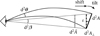 |
Fig. 1. Illustrating the difference between the geometrical magnification μ = d2θ/d2β and the observable magnification |
![Mathematical equation: $ \tilde{\mu}(z)=[\bar{D}{_{\text{ A}}}(z)/D{_{\text{ A}}}(z)]^2=({\text{ d}}^2\bar{A}/{\text{ d}}^2 A)\times({\text{ d}}^2{\boldsymbol{\theta}}/{\text{ d}}^2{\boldsymbol{\beta}}) $](/articles/aa/full_html/2021/11/aa40140-20/aa40140-20-eq21.gif)

Second, because of light deflection, the orientation of the source is tilted by an angle ι with respect to how it would be seen in FLRW. Because they are sub-tended by the same solid angle d2β, the tilted area d2A is larger than its untilted counterpart d2A⊥ = d2A × cos ι.
Summarising, the observable and geometrical magnifications are related as
![Mathematical equation: $$ \begin{aligned} \frac{\tilde{\mu }(z,\boldsymbol{\theta })}{\mu (z,\boldsymbol{\theta })} = \underbrace{\frac{\mathrm{d} ^2 \bar{A}}{\mathrm{d} ^2 A_\perp }}_{\mathrm{shift} } \underbrace{\frac{\mathrm{d} ^2 A_\perp }{\mathrm{d} ^2 A}}_{\mathrm{tilt} } = \frac{a^2[\bar{\eta }(z)] \, \bar{r}^2(z)}{a^2[\eta (z)]\, r^2(z)} \, \cos \iota . \end{aligned} $$](/articles/aa/full_html/2021/11/aa40140-20/aa40140-20-eq23.gif) (14)
(14)
We generally expect the shift to be the main driver of the difference between μ and  , because the tilt cos ι ≈ 1 − ι2/2 is a second-order quantity. Specifically, in the numerical results discussed in Sect. 4.1, the effect of tilt will always be sub-dominant; it will be precisely quantified in Sect. 4.3.
Physical origin of the shift. While μ is a pure-lensing quantity,  depends on other phenomena, such as time delays, Sachs-Wolfe (SW) and integrated Sachs-Wolfe (ISW) effects, or peculiar velocities. The latter in particular may lead to significant differences between μ(z) and
  at low redshift. If a source has, for instance, a centripetal peculiar velocity with respect to the observer, then its redshift is smaller compared to a comoving source at the same position. Thus, for a given redshift z its comoving distance must be slightly larger than the one that it would have if it were comoving,
  . Because the source event belongs to the observer’s past light cone, this also means that it happens slightly earlier,
  . At low z, this typically results in
  , implying that
  . The conclusion would be opposite if the peculiar velocity were centrifugal.
To be more specific, at first order in the peculiar velocities of the source, vs and of the observer, vs, the shift3 reads (Kaiser 1987; Sasaki 1987)
 (15)
(15)
where β is the unit vector in the background direction of the source. The 1/(ℋr) term in Eq. (15) shows that for sources at small distances,  may reach large values.
The quantity  is sometimes called ‘Doppler convergence’ (Bonvin 2008; Bolejko et al. 2013; Bacon et al. 2014), although it is unrelated to lensing. This expression and notation originate from the fact that we may define an observable distortion matrix
  , which is to the distortion matrix 𝒜 what
  is to μ. Namely, if
 (16)
(16)
where 𝒟 is the Jacobi matrix of the Sachs formalism (for example Fleury 2015, Sect. 2.2), then  . We may then introduce a convergence-shear decomposition of
  similarly to Eq. (4), thereby defining
  , to which
  is an important contribution.
Fixing other parameters. In the above, we have defined the observable magnification  at fixed redshift. This choice was made for concreteness, but the definition of
  could be adapted if we were to fix another parameter, such as the comoving radius, the emission time, or the affine parameter. A little intellectual challenge would consist in determining which light-cone slicing may ensure
  . To our knowledge, there is currently no answer to that particular question.
2.2.4. Amplification and luminosity distance
Small or remote sources, such as SNe or quasars, are generally unresolved by telescopes. In that context, the key observable is the observed flux, that is the total power received from the source per unit of telescope area, rather than the apparent size of images. We may define the amplification of a source β at z as the ratio of the observed flux S(z, β) with its unlensed counterpart  . By virtue of Etherington’s reciprocity law (Etherington 1933), and assuming a transparent Universe, the amplification is nothing but the total observable magnification,
![Mathematical equation: $$ \begin{aligned} \frac{S(z,\boldsymbol{\beta })}{\bar{S}(z)} = \tilde{\mu }_{\mathrm{tot} }(z,\boldsymbol{\beta }) \equiv \sum _{i=1}^{2n+1} |{\tilde{\mu }[z,\boldsymbol{\theta }_i(\boldsymbol{\beta })]}|. \end{aligned} $$](/articles/aa/full_html/2021/11/aa40140-20/aa40140-20-eq45.gif) (17)
(17)
By definition of the luminosity distance DL, we also have
![Mathematical equation: $$ \begin{aligned} \tilde{\mu }_{\mathrm{tot} }(z,\boldsymbol{\beta }) = \left[\frac{\bar{D}_{\mathrm{L} }(z)}{D_{\mathrm{L} }(z,\boldsymbol{\beta })}\right]^2\cdot \end{aligned} $$](/articles/aa/full_html/2021/11/aa40140-20/aa40140-20-eq46.gif) (18)
(18)
This could seem to be at odds with Eq. (11) and the well-known distance-duality relation DL = (1 + z)2DA. This apparent paradox is due to the fact that we have defined DA for a single image, while DL accounts for all the images of a given source. The two approaches are reconciled if we consistently distinguish between image-based definitions and source-based definitions. For example, we could define the area distance of a multiply imaged source DA(z, β) from the total apparent area occupied by all its images. In that case ![Mathematical equation: $ [\bar{D}{_{\text{ A}}}(z)/D{_{\text{ A}}}(z,{\boldsymbol{\beta}})]^2=\tilde{\mu}{_{\text{ tot}}}(z,{\boldsymbol{\beta}}) $](/articles/aa/full_html/2021/11/aa40140-20/aa40140-20-eq47.gif) consistently with distance duality.
consistently with distance duality.
Finally, we note that Eq. (17) is only valid if one compares the background and perturbed fluxes at the same redshift z. Had we compared the two situations, for instance, at fixed affine parameter, the background and perturbed redshift would have differed, which would have affected fluxes through the energy and the reception rate of individual photons.
2.3. Averaging in cosmology
The interpretation of cosmological observations, and their confrontation with theoretical predictions, involve various notions of averaging, which are non-trivially related in the presence of gravitational lensing. We review here the relevant definitions and properties of cosmological averages, elaborating on Bonvin et al. (2015b), Kaiser & Peacock (2016), Fleury et al. (2017a).
Importantly, from now on we shall neglect multiple imaging, except explicitly stated otherwise. Thus, the lens mapping θ ↦ β is assumed to be a diffeomorphism of 𝕊2, and the resulting magnifications are positive. In that context, there is no difference between signed, absolute, and total magnifications any more. We may also treat observable magnification and amplification as synonyms, both denoted  . This assumption is justified by the relatively rare occurrence of strong lensing from a cosmological perspective, and by the huge gain of simplicity that it brings to the discussions of this section.
2.3.1. Directional averaging
Let X(θ) be an observable in the direction θ on the observer’s celestial sphere, such as the temperature anisotropies of the cosmic microwave background, or the apparent surface density of galaxies. Directional averaging ⟨…⟩d corresponds to a statistical average of X(θ) where all the observation directions θ have the same statistical weight; the average is thus weighted by the image solid angle d2θ,
 (19)
(19)
One may ask how lensing affects directional averages, in particular for distance measurements. We first note that, by virtue of Eq. (7), the directional average of the inverse geometric magnification is unity,
 (20)
(20)
This property is exact and applies to any slicing of the light-cone. However, as pointed out in Sect. 2.2.3, Eq. (20) has only little observational relevance, because the actually observable quantity is  , which differ from μ by the shift and tilt described in Fig. 1. Despite that concern, we may still conclude that
 (21)
(21)
in the limit where the tilt/shift corrections are sub-dominant compared to the most relevant gravitational-lensing effects.
Unlike Eq. (20), the accuracy of Eq. (21) depends on which parameter is fixed in the definition of  . For instance, Kibble & Lieu (2005) argued that
  was accurate for sources at fixed affine parameter λ; this was checked numerically with ray tracing in post-Newtonian cosmological modelling (Sanghai et al. 2017). However, we shall see in Sect. 4.2.5 that the use of the affine parameter is quite risky at very high redshift. If instead the redshift is kept fixed, then significant departures from
  are expected at low z due to peculiar velocities.
2.3.2. Source-averaging and areal averaging
We now consider an observable Y which is associated with a specific population of sources, such as the distance to type-Ia supernovae or the Lyman-α absorption in quasar spectra. The natural averaging procedure associated with such an observable is called source averaging ⟨…⟩s, and is defined as
 (22)
(22)
where N denotes the number of observed sources, and in the second equality we took the continuous limit. The difference with directional averaging is that the sky is not necessarily homogeneously sampled. Clearly, if the sources are not homogeneously distributed in the Universe, then their projected density N−1d2N/d2θ tends to favour some regions of the sky more than others, thereby breaking the apparent statistical isotropy.
But even if sources are homogeneously distributed in space, gravitational lensing implies that they do not evenly sample the observer’s sky. Indeed, lensing tends to make light beams ‘avoid’ over-dense regions of the Universe, thereby favouring under-dense regions in source-averages. This specific effect may be captured in the notion of areal averaging. For example, if all the sources are observed at the same redshift z, we may define the areal average of Y as
 (23)
(23)
with Σ(z) the surface of constant redshift z and A(z) its total proper area. The definition must be adapted if the sources are observed on other slices of the light cone, for instance all at the same emission time η or affine parameter λ.
Using the area distance,  , we may convert areal averages in terms of directional averages as follows,
 (24)
(24)
from which we immediately conclude, substituting  , that
 (25)
(25)
by virtue of Eq. (21). Areal averaging exactly coincides with source-averaging if the sources are homogeneously distributed on Σ(z), because then the number of observed sources scales as the area that they occupy, so that  . If not, corrections arise from the correlation between the fluctuations of the density of sources and the amplification; further corrections such as redshift-space distortions, must also be accounted for if the sources are observed in redshift bins (Fleury et al. 2017a; Fanizza et al. 2020). Such discrepancies between source-averaging and areal averaging typically remain below 10−5, and hence they may be neglected. Combining this approximation with Eq. (25) then yields
 (26)
(26)
Equation (26) was shown to be accurate at the 10−3 level up to z = 3 by Adamek et al. (2019).
2.3.3. Ensemble averaging and cosmic variance
We shall close this discussion with the notion of ensemble averaging. Within the standard lore, we envisage all cosmological structures as originating from quantum fluctuations in the primordial Universe (Peter & Uzan 2013). From that point of view, ϕ(η, x) is a particular realisation of an intrinsically stochastic field, which is believed to be initially Gaussian. In that framework, the ensemble average of any field Z(η, x) that depends on ϕ, which we may simply denote as ⟨Z(η, x)⟩, would be its expectation value over an infinite number of realisations the Universe.
Contrary to directional, areal, or source-averages, ensemble-averaging is thus a strictly theoretical procedure, which is nevertheless used in any cosmological prediction. Ensemble averaging may be connected to other averaging procedures via the ergodicity principle. Which observable averaging is mimicked by ensemble averaging then depends on which quantities are kept fixed when making multiple realisations of the Universe as illustrated in Fig. 2. For example, if the observed direction of light θ and redshift z are kept fixed, then we get directional averaging,
 (27)
(27)
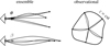 |
Fig. 2. Correspondence between ensemble averaging and observational averaging procedure depends on which quantity is kept fixed. |
because any θ is virtually affected the same statistical weight. In this scenario, the source position β may change from one cosmic realisation to another. An alternative scenario would consist, on the contrary, in fixing β while allowing θ to vary from one realisation to another; this yields
 (28)
(28)
We may divide the above with ⟨μ−1⟩d if directional average is taken on a fraction of the sky only. Other possibilities would consist in fixing another parameter than the redshift, such as time or affine parameter, which would correspond to averaging across other slices of the light cone.
Importantly, ergodicity is sensible only if the region of the Universe over which an observational averaging is performed is statistically homogeneous. In other words, there should not be super-sample inhomogeneity modes. Such an assumption is not satisfied in the standard lore, which predicts inhomogeneity modes at all scales. Thus, any observational average is subject to an irreducible source of uncertainty, called cosmic variance. Equations (27) and (28) only hold up to cosmic variance.
2.4. Biased distance measurements
Equations (21) and (26) show than only very specific quantities are (almost) unbiased by cosmic inhomogeneities; in particular, most distance measurements happen to be biased. We describe here the nature and amplitude of these biases.
We introduce for convenience the dimension-less distance
 (29)
(29)
Because d is a non-linear function of  , it exhibits a statistical bias for both directional and source-averaging. For directional averaging we may expand d at second order in
  and use Eq. (21) to get
![Mathematical equation: $$ \begin{aligned} \langle {d(z)}\rangle _{\mathrm{d} }-1 \approx -\frac{1}{8} \left\langle {[\tilde{\mu }^{-1}(z)-1]^2}\right\rangle _{\mathrm{d} } < 0. \end{aligned} $$](/articles/aa/full_html/2021/11/aa40140-20/aa40140-20-eq69.gif) (30)
(30)
Similarly, for areal or source-averaging we may expand d in terms of  which, together with Eq. (26) yields
![Mathematical equation: $$ \begin{aligned} \langle {d(z)}\rangle _{\mathrm{s} }-1 \approx \frac{3}{8} \left\langle {[\tilde{\mu }(z)-1]^2}\right\rangle _{\mathrm{s} } > 0. \end{aligned} $$](/articles/aa/full_html/2021/11/aa40140-20/aa40140-20-eq71.gif) (31)
(31)
The biases appearing in Eqs. (30) and (31) are not independent, and are usually expressed in terms of the convergence. Indeed, if the amplification is expressed in terms of some convergence and shear similarly to Eq. (5), that is, ![Mathematical equation: $ \tilde{\mu}=[(1-\tilde{\kappa})^2-|\tilde{\gamma}|^2]^{-1} $](/articles/aa/full_html/2021/11/aa40140-20/aa40140-20-eq72.gif) , then at second order in
, then at second order in  ,
,
 (32)
(32)
Since  is a second-order quantity, the difference between its directional, source-, or ensemble-average would be of higher order, and hence it should not matter much which averaging procedure is considered when substituting
  in Eqs. (30) and (31). Furthermore, if we neglect again the shift and tilt corrections4 and write
  , then we simply have
 (33)
(33)
 (34)
(34)
If Eq. (34) is applied at the redshift of the CMB, z* ≈ 1100, and κ(z) is computed from linear perturbation theory, then the corresponding bias reaches the percent level. This is how Clarkson et al. (2014) concluded that the standard analysis of the CMB, which does not account for such a bias, might be flawed. That conclusion was shown to be incorrect by Bonvin et al. (2015a), Kaiser & Peacock (2016), because the analysis of the CMB is in fact not sensitive to ⟨d(z*)⟩s. However, supernova cosmology is. In supernova surveys, it is customary to use the distance modulus rather than the luminosity distance as a distance measure; its perturbation due to inhomogeneities reads Δm = 5log10d, and hence its source-averaged bias is
![Mathematical equation: $$ \begin{aligned} \langle {\Delta m(z)}\rangle _{\mathrm{s} } \approx \frac{5}{4\ln 10} \left\langle {[\tilde{\mu }(z)-1]^2}\right\rangle _{\mathrm{s} } \approx \frac{5}{\ln 10} \left\langle {\kappa ^2(z)}\right\rangle . \end{aligned} $$](/articles/aa/full_html/2021/11/aa40140-20/aa40140-20-eq80.gif) (35)
(35)
For z < 2, this bias remains below 10−3 and hence is negligible in current SN surveys, except for reconstructions of the evolution of the dark-energy equation of state (Fleury et al. 2017a). It would be easily removed if next-generation surveys were using  instead of magnitude as a distance indicator.
We finally note that all the above only holds in a transparent Universe. If this assumption is relaxed, then distance measurements may be further biased by selection effects. For instance, in a Universe made of opaque matter lumps, observed light beams do not evenly sample the density field – they experience an effectively under-dense Universe. This result in an effective de-focussing of light as originally described by Zel’dovich (1964), later generalised by Dashevskii & Slysh (1966) and Dyer & Roeder (1974) on the basis of Einstein-Straus Swiss-cheese models (Kantowski 1969; Fleury 2014). The resulting bias on luminosity distance measurements typically reaches 10% at z = 1 for very lumpy models (Fleury et al. 2013). In Okamura & Futamase (2009), the authors made an attempt to determine the fraction of such opaque lumps based on the halo model of Sheth & Tormen (1999). To date, however, there is no compelling evidence of any large effect of opaque lumps on distance measurements in our Universe (Helbig 2020).
2.5. Reformulation: the area of light-cone slices
We may now rephrase the average-amplification rules (21) and (26) in terms of the area of light-cone slices, such as surfaces of constant redshift. We consider for instance the directional average of the inverse amplification:
 (36)
(36)
where in the last equality we introduced the area A(z) of the surface of constant redshift, Σ(z), as well as its background counterpart  . Equation (36) thus tells us that
  would be equivalent to
  ; meaning that the area of iso-z surfaces is mostly unaffected by inhomogeneities.
Although it may seem quite natural, the last equality of Eq. (36) is, in fact, not obvious. In the background FLRW space-time,  is a sphere (in comoving coordinates) at constant cosmic time; hence its proper area is clearly
  . But things are less clear in the inhomogeneous Universe, where Σ(z) is wrinkly and is not limited to a constant-time hypersurface. The definition of its proper area A(z) is then subject to several questions about its uniqueness, if it is frame-dependent and how it relates to the angular distance. We propose to clarify these subtleties below.
2.5.1. Surfaces of constant redshift and their area
Surfaces of constant redshift, Σ(z), correspond to a particular slicing of the light cone 𝒞 of the observation event O, as illustrated in Fig. 3. We note that this slicing is generally not performed at constant time, η(z)≠ const. This last property raises the question of how to actually define the proper area of Σ(z).
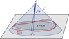 |
Fig. 3. Surface of constant redshift, Σ(z) (red), is a particular slicing of the light cone 𝒞 (blue) that is not included in constant-time hyper-surfaces (grey). We represented light rays as straight lines for simplicity. |
Let d2x be the element of Σ(z) subtended by the solid angle d2θ at O. For causality reasons, d2x must be space-like; thus, there exists a frame such that d2x is strictly spatial. We shall call it the ‘natural frame’5 of d2x, and define the area d2Az of d2x in that frame. Applying that construction to all elements d2x of Σ(z) and integrating over them then defines its total area A(z).
Now that we have defined the area of an iso-z surface, we shall see how it relates to the angular distance DA(z). For that purpose, we note that d2x is orthogonal to direction of light propagation in its natural frame. We shall now prove this point. We may see 𝒞 as the hyper-surface defined by all the events that are in phase with O, for a spherical wave converging at the observer. If w denotes the phase of that wave and kμ = ∂μw is the associated wave four-vector, then any displacement dxμ across 𝒞 satisfies kμdxμ = dw = 0. This applies, in particular, to any dxμ ∈ d2x ⊂ Σ(z)⊂𝒞. In the natural frame of d2x, this four-dimensional orthogonality becomes three-dimensional because dx0 = 0; in other words, k ⋅ dx = 0, where k is the wave-vector in the natural frame.
The spatial orthogonality between k and d2x implies that d2x forms a Sachs screen space in its natural frame. Thus, d2Az is not only the proper area of d2x, but also the cross-sectional area of the light beam subtended by d2θ in that frame. By virtue of Sachs’ shadow theorem (Sachs 1961, see also Sect. 2.1.2 of Fleury 2015), the area of a beam is independent of the frame in which it is evaluated, as long as it is projected on a Sachs screen. This unique notion of a beam’s cross-sectional area then defines the angular distance according to
 (37)
(37)
This confirms that the area of Σ(z) is indeed related to the angular distance as  , thereby validating the last equality of Eq. (36).
We finally note that the above reasoning actually applies to any slice of the light cone. In other words, for any parameter p such that the iso-p surface Σ(p) is space-like (p may stand, for instance, for the affine parameter λ, time η, the comoving radius r, etc.) the area of the element d2x subtended by the solid angle d2θ reads  and the total area of the iso-p surface is
 (38)
(38)
2.5.2. The photon-flux conservation argument
In the spirit of the second part of Weinberg (1976), we may also connect the area-averaged amplification to A(z) on the basis of photon conservation. Let F0 be the total number of photons received per unit time by an observer. If the photon number is conserved, then the same photons crossed Σ(z) at a rate Fz = (1 + z)F0, where the (1 + z) factor accounts for time dilation. Importantly, the latter relation holds regardless of the geometry of Σ(z); in other words,  .
.
Now, the photon flux may be written as
 (39)
(39)
where n is the outgoing normal to Σ(z), J is the photon flux density vector, and in the second equality we used that in its natural frame n is aligned with k and hence to J. Since J = Π/(ℏω), where  is the Poynting vector, we conclude that
  . Combining this with
  then yields
 (40)
(40)
Therefore, Eq. (25) is equivalent to stating that inhomogeneities do not affect the area of iso-z surfaces. We stress again here that Weinberg’s photon-flux-conservation argument does not imply that  , but rather shows that such an equality is equivalent to
  .
.
2.5.3. CMB and the area of the last-scattering surface
Hitherto, our discussion has been focused on surfaces of constant redshift because of their connection with observational averages. The archetypal application would be the analysis of the Hubble diagram in a non-homogeneous Universe, which involves the source-averaged distance modulus. However, shall we be more interested in the analysis of the CMB than in SNe, more relevant would be the last-scattering surface (LSS) and its area A*.
The area of the LSS is a relevant quantity indeed. As illustrated in Fig. 4, A* essentially drives how many sound horizons rs the observer may count in the CMB, and hence their average angular size θ* which is one of the main direct CMB observables. The problem is then to estimate to which extent is A* affected by the inhomogeneities of our Universe. Following KP16, we shall approximate the LSS as a surface of constant time6, Σ(η*). By virtue of Eq. (38) for p = η*, we have  where the departure from strict equality stems from the difference between
  and μ(η*), that is from the small shift and tilt effects emphasised in Sect. 2.2.3.
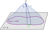 |
Fig. 4. Last scattering surface, approximated as a constant-time slice Σ(η*) of the light cone 𝒞. Its area is connected to the number of sound horizons rs that appear on the observer’s CMB, and hence to its average apparent size θ*. |
From a pedagogical point of view, surfaces of constant time Σ(η) are very attractive because their natural frame (in the sense of Sect. 2.5.1) is the comoving frame. Indeed, for any displacement dxμ ∈ Σ(η) we have by definition dx0 = 0 in comoving coordinates. Because of this, the shift and tilt corrections to the area A* of the LSS can be made particularly explicit. Expressing A* as the area of a polar surface, we have indeed
 (41)
(41)
 (42)
(42)
where  is the comoving radial coordinate of the point of LSS with angular coordinates β, which is generally shifted with respect to its background counterpart
  . The angle ι*(β) is the tilt between the normal to the LSS and the radial direction; it encodes the wrinkles of the LSS which tend to increase its area. Recall that β denotes the ‘true’ angular position of a point of the LSS, not to be confused with the direction θ in which that point would be observed.
In order to get a theoretical prediction for  , we may expand Eq. (41) at second order in cosmological perturbations, and assume ergodicity to turn integrations over β into ensemble averages (see Sect. 2.3.3). This yields
 (43)
(43)
with  .
.
KP16 proposed a quite intuitive analysis of the shift term, δr*; we shall paraphrase their idea here, while further details and minor corrections are given in Appendix C. The first effect of inhomogeneities is the presence of the gravitational potential ϕ, which changes the effective (coordinate) speed of light as
 (44)
(44)
As a consequence, during a fixed travel time η0 − η, the comoving distance travelled7s is slightly changed, s(η) = η0 − η + δs(η). At the LSS, this reads
![Mathematical equation: $$ \begin{aligned} \delta s_*(\boldsymbol{\beta }) = \int _{\eta _*}^{\eta _0} \mathrm{d} \eta \; 2\phi [\eta , \boldsymbol{x}(\eta )], \end{aligned} $$](/articles/aa/full_html/2021/11/aa40140-20/aa40140-20-eq110.gif) (45)
(45)
where x(η) is the photon trajectory connecting the observer to the point β of the LSS. We note that this is nothing but the usual Shapiro time delay seen from a different point of view.
Second, because of gravitational lensing, light rays are wiggly, and hence the comoving radius r that they reach after travelling a comoving distance s is slightly smaller than s. At the LSS we may write r* = s* + δrgeo, with
![Mathematical equation: $$ \begin{aligned} \delta r_{\mathrm{geo} }(\boldsymbol{\beta }) = \int _0^{s_*} \mathrm{d} s \; [\cos \iota (s)-1] \approx -\frac{1}{2}\int _0^{\bar{r}_*} \mathrm{d} r \; \iota ^2(r), \end{aligned} $$](/articles/aa/full_html/2021/11/aa40140-20/aa40140-20-eq111.gif) (46)
(46)
at second order in perturbations, and where ι is the angle made between the instantaneous photon propagation direction and the axis spanned by β. It coincides with ι* at the LSS.
When both effects (time delay and wiggles) are taken into account, the radial shift of the LSS with respect to its background counterpart reads
 (47)
(47)
We note that δs* is first-order, while δrgeo is second-order in cosmological perturbations. It is thus essential to go beyond the Born approximation when evaluating δs* for consistency. Because of that hierarchy, δs* may also be considered the main driver of the wrinkles ι* of the LSS.
Once ensemble average is taken, Eq. (43) yields
 (48)
(48)
 (49)
(49)
where Pϕ denotes the power spectrum of the gravitational potential. More details can be found in Appendix C. Equation (48) agrees with Eq. (A.44) of KP16, albeit obtained via a slightly different path.
2.6. Summary and goal of the remainder of this article
Inhomogeneities may bias cosmological observations, notably via the effect of gravitational lensing on distance measurements. Biases depend on the notion of averaging that is involved. By virtue of the inverse-magnification integral ⟨μ−1⟩d = 1, some specific observables are expected to be almost unbiased: ⟨d2(z)⟩d ≈ 1/⟨d−2(z)⟩s ≈ 1. Other combinations of d, such as the magnitude, generally exhibit a potentially much larger bias, on the order of ⟨κ2⟩. Departures from the exact ⟨d2(z)⟩d = 1 stem from  and may be interpreted as being due to shifts and tilts of iso-z surfaces with respect to their background counterpart. Apart from these shift and tilt effects, the area of iso-z surfaces is unaffected by inhomogeneities. An equivalent reasoning may be applied to other slices of the light cone, such as surfaces of constant time whose area is relevant for CMB observations.
In the remainder of this article, we propose to numerically evaluate: (i) the accuracy of ⟨d2(z)⟩d ≈ 1/⟨d−2(z)⟩s ≈ 1; (ii) the amplitude of the 𝒪(⟨κ2⟩) bias on other observables; (iii) the performance of the prediction (48) for the area of iso-η surfaces. Our investigation will be based on accurate ray tracing in a high-resolution N-body simulation, so as to fully capture non-linear effects which are difficult to control in a pure-theory approach.
3. Numerical methods
In this section, we present the numerical set-up and the various tools that are used to obtain the results reported in Sect. 4.
3.1. Simulation
We use the N-body code RAMSES (Teyssier 2002; Guillet & Teyssier 2011) with dark matter (DM) only. RAMSES uses a Particle-Mesh with Adaptive-Mesh-Refinement (PM-AMR) method, which computes the evolution of the gravitational potential and density field from particles and gravity cells. AMR allows one to probe high-density regions and hence the highly non-linear regime of structure formation.
The simulation’s box comoving length is 2625 h−1 Mpc with 40963 particles in a ΛCDM cosmology with WMAP-7 best-fit parameters (Komatsu et al. 2011), namely h = 0.72, total-matter density Ωm = 0.25733, baryon density Ωb = 0.04356, radiation density Ωr = 8.076 × 10⁻⁵, spectral index ns = 0.963 and power-spectrum normalisation σ8 = 0.801. The corresponding DM-particle mass is 1.88 × 10¹⁰ h−1 M⊙. The initial power spectrum is computed with CAMB (Lewis et al. 2000). Initial conditions are generated using a 2LPT version of MPGRAFIC (Prunet et al. 2008) to avoid transients (Scoccimarro 1998), which allows us to start the simulation at z = 46.
Fidler et al. (2015, 2016) showed that Newtonian N-body simulations, such as the one used in this article, yield physical quantities computed in the so-called N-body gauge. In principle, a small relativistic correction must be applied to translate such results into the Newtonian gauge (Chisari & Zaldarriaga 2011). We choose to neglect these corrections, and hence we identify the coordinates and the gravitational potential computed from the simulation with the coordinates and metric perturbation ϕ in Eq. (1).
3.2. Light cones
To produce light cones from our simulation we use the onion-shell method (Fosalba et al. 2008; Teyssier et al. 2009). At each synchronisation (coarse) time step of the simulation, we output a thin spherical shell whose mean radius is the comoving distance to a central observer at the snapshot time. The shells contain all the required information about the particles (positions and velocities) and about the grid cells (gravitational potential and acceleration). Furthermore, the shells are produced with a non-zero thickness, in the sense that every spatial cell appears at different times, which allows us to compute time derivatives.
We produce three different light cones for a given observer at the centre of the simulation, which correspond to three different depths and sky coverage. The simulation box size allows us to build a full-sky cone up to a radius equal to half the box length, corresponding to z ≲ 0.5. Going further would imply that some parts of the cone would repeat due to the periodic boundary conditions of the simulation. Such replication effects are suppressed by reducing the angular width of the light cone beyond z ≈ 0.5. An intermediate narrow cone is built up to z = 2 with a sky coverage of 2500 deg2, while our deep narrow cone goes up to z = 10 covering 400 deg2. The cones are oriented so that light rays do not cross the same structures at different times.
Haloes on the light cones are identified using the parallel Friend-of-Friend (PFoF) code (Roy et al. 2014) with linking length b = 0.2 and at least 100 DM particles. A halo’s position is defined from its centre of mass, while its velocity is defined as the mean velocity of the particles that it contains. The properties of the DM haloes of the present simulation have been studied in the appendix of Corasaniti et al. (2018).
We choose to model neither the haloes’ intrinsic luminosity, nor the luminosity threshold for their detection by the observer. Thus, the results presented in this article exploit all the available data within the redshift ranges of interest.
3.3. 3D relativistic ray tracing
Observables are extracted from the light cones using a fully relativistic ray-tracing procedure based on the MAGRATHEA library (Reverdy 2014). Ray-tracing is performed backwards, that is, towards the past starting from the observation event where λ = 0. Initial conditions are fixed by the observation direction n and by setting k0 = 1. This means that the affine parameter coincides with conformal time at O. The observer is chosen to be comoving, meaning that its peculiar velocity is set to zero, vo = 0. This implies that ki ∝ ni, where the proportionality factor is such that kμkμ = 0.
From these initial conditions, the geodesic Eqs. (2) and (3) are integrated numerically with a fourth-order Runge-Kutta integrator. Specifically, photon trajectories are computed within the 3D AMR structure with four steps per AMR cell. Since the underlying N-body code uses a Triangular Shaped Cloud (TSC) interpolation scheme, we use an inverse TSC to estimate the gravitational potential and acceleration at the exact position of a photon. Using another interpolation method may lead to inconsistencies, such as self-accelerating particles.
The 3D TSC scheme requires 27 cells with the same refinement level to interpolate the value of a field at a position x. In practice, we start with the finest level, that is, the level of the smallest cell that contains x; if there are less than 27 neighbouring cells with the same refinement level, then we try again with the next coarser level, and so on.
We stop the ray tracing if (and only if) that operation is impossible even at the coarse level, which means that the ray reaches the limits of our numerical background light-cones (described in Sect. 3.2) and there is no more data available to pursue its propagation. Importantly, we save all the information about every integration step of each ray’s trajectory. Besides, rays are traced irrespective of the structures that they encounter; in other words, matter is assumed to be transparent.
3.4. Infinitesimal beams
The most common way to numerically evaluate the distortion matrix 𝒜 is based on the multi-plane lensing formalism (Blandford & Narayan 1986), where the matter distribution near the line of sight (LOS) is projected onto various planes which are then treated as thin lenses (Jain et al. 2000; Hilbert et al. 2009). Here we want to fully exploit the 3D information of the RAMSES AMR octree. For that purpose, a first option consists in integrating the projected Hessian matrix ∇a∇aϕ of the gravitational potential along the actual trajectories of light rays,
![Mathematical equation: $$ \begin{aligned} \mathcal{A} _{ab} = \delta _{ab} - \frac{2}{c^2}\int ^{r_{\mathrm{s} }}_0 \mathrm{d} r\;\frac{(r_{\mathrm{s} }-r)r}{r_{\mathrm{s} }}\nabla _a\nabla _b\phi [\eta (r),\boldsymbol{x}(r)], \end{aligned} $$](/articles/aa/full_html/2021/11/aa40140-20/aa40140-20-eq116.gif) (50)
(50)
where rs is the comoving distance to the source, a, b take the values 1, 2, and the two-dimensional gradient ∇a is transverse to n (to the LOS). In practice, the 3D Hessian ∂i∂jϕ is computed on the mesh, and then converted in spherical coordinates to extract its angular (transverse) part ∇a∇bϕ.
We shall refer to this approach as the ‘infinitesimal-beam method’, because it describes the distortions of an infinitesimal light source. We note that this way of computing 𝒜 is comparable to the method used in RAY-RAMSES (Barreira et al. 2016), except that here ∇a∇bϕ is evaluated on the actual ray trajectory rather than on the background trajectory. In other words, we do not resort to the Born approximation.
3.5. Ray bundles and finite-beam effect
The second option to compute the distortion matrix 𝒜 is based on a bundle of rays (a minima three), which may be seen as a finite light beam subtended by an extended light source (Fluke et al. 1999; Fluke & Lasky 2011). In that ‘ray-bundle method’, each ray is accompanied with four auxiliary rays making an angle ε with the central one, as depicted in Fig. 5. The components of 𝒜 are then computed from finite coordinate differences between the rays, rather than from gradients.
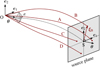 |
Fig. 5. Ray-bundle method. A central light ray (dotted line) is accompanied with four auxiliary rays A, B, C, D (red solid lines). Each auxiliary ray makes an angle ε at O with respect to the central ray. The distortion matrix is estimated by comparing the relative positions of the auxiliary rays in a plane orthogonal to the line of sight θ. |
More precisely, our method goes as follows: First, stop the central ray when the relevant parameter (such as redshift, time or comoving distance) has reached the desired value; this defines the fiducial source event S. Second, stop the auxiliary rays at the same affine parameter λ as the central ray’s at S. This criterion is arbitrary and other possibilities are implemented in the code. Third, project the relative positions of the auxiliary rays on some source plane. For simplicity, we chose it to be orthogonal to the LOS8θ. This defines the transverse separation ξ between the auxiliary rays and the central one.
Our estimator  for the distortion matrix is then motivated by the fact that if two rays separated by a small Δθ at O should have angular coordinates differing by
  ,
,
 (51)
(51)
where r is the radial position where the central ray was stopped, and e1, e2 are unit vectors defining the initial separation of the auxiliary rays with respect to the central ray.
We note that the choices made in step 2 and 3 induce a spurious tilt in our estimate of the distortion matrix. We have checked that the effect of this tilt is negligible in all the results involving  in this article. The specific analysis of the tilt in Sect. 3.8, which require a better accuracy, will rely on a different method.
The finite separation of the rays in the bundle method may cause some discrepancies with the infinitesimal-beam approach. Those may be quantified using the finite-beam formalism developed by Fleury et al. (2017b, 2019a,b)9. In particular, the finite-beam corrections to the angular power spectrum of convergence, Pκ, and shear, Pγ, are found to read
 (52)
(52)
 (53)
(53)
where Pκ, γ(ℓ; 0) denote the power spectra computed with the infinitesimal-beam approach described in Sect. 3.4.
The complete derivation of Eqs. (52) and (53) is provided in Appendix B; it relies on the weak-lensing, flat-sky, and Limber approximations. We note that Eqs. (52) and (53) differ from the results highlighted in Fleury et al. (2019a, Eqs. (120) and (121)), because they correspond to different beam geometries. The latter were computed from the distortions of circular beams, while the former correspond to square-shaped beams as depicted in Fig. 5.
Figure 6 compares the predictions of Eqs. (52) and (53) with ray tracing. Three different beam semi-apertures are considered: ε = 35 arcmin, 3.5 arcmin and 0.35 arcmin, to which we may add ε = 0 corresponding to infinitesimal beams. For each value of ε but 0, we compute the convergence and shear using the ray-bundle method, at z = 1.95 on the intermediate narrow light cone, and for LOS dictated by HEALPIX (Górski et al. 2005). Power spectra are extracted using POLSPICE (Szapudi et al. 2001; Chon et al. 2004), so as to correctly allow for the angular selection function associated with the narrow cone’s geometry.
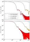 |
Fig. 6. Finite-beam corrections to the angular power spectrum of convergence (top panel) and shear (bottom panel) at z = 1.95, for different semi-aperture sizes. Black lines indicate the theoretical predictions of Eqs. (52) and (53), while coloured lines indicate ray-tracing results. |
Power-spectrum estimates from HEALPIX turn out to be robust until ℓ ≈ nside10 Since finite-beam effects typically kick in from ℓ ∼ ε−1, we set nside = 4096 for ε = 35arcmin and ε = 3.5 arcmin, while we set nside = 8192 for the smallest beam size ε = 0.35 arcmin, so as to ensure that the power spectra are reliable at the scales of interest.
The excellent agreement between Eqs. (52) and (53) and ray tracing, as shown in Fig. 6, is the first numerical evidence of the accuracy of the finite-beam formalism. This confirms that the finite-beam corrections that may arise in the present work are well understood and under control. In particular, the damping of Pκ(ℓ; ε) Pγ(ℓ; ε) is expected to slightly reduce the variance of convergence and shear, which are involved in distance biases. Such effects will not change the conclusions of our analysis.
Except otherwise stated, in the remainder of this article we set ε = 0.35 arcmin. Smaller beam sizes are excluded because they would exceed the resolution of the simulation.
3.6. Producing observables for statistical averages
We now turn to the generation of observables, for the purpose of computing statistical averages. As seen in Sect. 2, directional averaging and source averaging are distinct operations for which different numerical techniques must be applied.
3.6.1. HEALPIX maps for directional averages
Directional averaging consists in affecting equal weights to all directions of the observer’s sky. This condition is easily satisfied by dividing the sky into pixels of equal area, which is the purpose of HEALPIX. In order to estimate the directional average ⟨X⟩d of an observable X, we thus shoot a ray bundle in each direction θ dictated by HEALPIX, compute X(θ), and take their average.
3.6.2. Halo catalogues for source averaging
Source averaging gives the same statistical weight to each source on the observer’s light cone. Thus, computing source averages requires to produce a source catalogue, and to determine the null geodesic that connects each source to the observer.
In this work, sources are identified with the DM haloes, which are extracted from the simulation as described in Sect. 3.2. Geodesic identification, besides, follows Breton et al. (2019) (see also Adamek et al. 2019). In a nutshell, a photon is shot towards the comoving direction of a source; due to gravitational lensing the photon generally misses the source, so that LOS must be corrected and the operation iterated upon convergence at the source (for an illustration, see Fig. 1 in Breton et al. 2019). This procedure eventually yields the full trajectory of light for each source, as well as its observed position. We note that we do not account for multiple images of the same source, meaning that we stop the geodesic-finding algorithm as soon as one valid ray is found.
From the N-body code we also know the gravitational potential and velocity of each source in the catalogue. This data notably allow us to accurately compute the redshift, accounting for all the special- and general-relativistic effects at first order in the metric perturbation. The quantitative features of the mocks11 used in this work are summarised in Table 1.
Three light cones are used for the present work.
3.7. Surfaces on the light cone
In this article, we shall consider various ways to slice the observer’s past light cone, depending on which parameter is fixed; namely: Surfaces of constant redshift (iso-z), constant time (iso-η), constant comoving distance travelled (iso-s), and constant affine parameter (iso-λ). In the background FLRW model, all these surfaces are spherical and correspond to each other following specific one-to-one relations. These are denoted with an over-bar; for instance,  is the background redshift on the background iso-η surface. In practice, we determine these background relations by shooting a single ray in the simulation with ϕ = 0.
In the inhomogeneous case, the surfaces are determined by shooting rays in directions θ set by HEALPIX. Since all the properties of the ray and its location are saved at each integration step, it is straightforward to determine the perturbed surfaces, such as iso-η surfaces x(η), as well as the value of all the other parameters across the surfaces, so that  . The comoving distance travelled s is computed at each integration step according to si + 1 = si + |xi + 1 − xi|.
Subtleties arise in the case of iso-z surfaces. The significant contribution of peculiar velocities to the observed redshift raises two issues: First, since velocities are only defined for particles, interpolation on the grid is necessary to estimate z at each time step. For that purpose, we use a TSC interpolation using all the DM particles in the redshift range of interest with a buffer zone. Second, it may happen that a light ray meets the same redshift multiple times during its propagation. In other words, the function λ ↦ z(λ, θ) is not one-to-one in the inhomogeneous Universe; iso-z surfaces are not uniquely defined. In this work we restrict the analysis to the two extremal iso-z surfaces, namely the closest to the observer {x[rmin(z, θ),θ]}, and the farthest from the observer {x[rmax(z, θ),θ]}. We denote these surfaces Σ−(z) and Σ+(z) respectively.
3.8. Computing the area of wrinkly iso-η surfaces
In order to check the theoretical predictions of Sect. 2.5.3 regarding the area of the LSS, and more generally of the iso-η surfaces, we need to numerically evaluate the expression
 (54)
(54)
where β denotes the ‘true’ position of a point of the iso-η surface, as opposed to the direction θ in which it would be observed. Such a computation thus requires the numerical determination of r(η, β) and its gradient ∂r/∂β.
In practice, however, we have a more direct access to r(η, θ) because the iso-η surface is determined by ray shooting (see Sect. 3.7), which yields r(η, θ) and β(η, θ) for each θ of a HEALPIX map. One could in principle compute r(η, β) by finding the null geodesics between the observer and the direction β at each iso-η surface, but this procedure would be computationally expensive. Another option consists in directly building a lower-resolution HEALPIXβ-map, such that in each pixel r(η, β) is the average of the r(η, θ) for which β(η, θ) falls into that pixel.
An even cheaper possibility consists in using the fact that the conversion between θ and β is dictated by lensing quantities, which we do compute for each ray. We shall adopt this method here. Specifically, in terms of θ, Eq. (54) reads
 (55)
(55)
 (56)
(56)
The quantities r, 𝒜, μ are indeed evaluated in each direction θ of our HEALPIX maps, thereby making the computation of A(η) much easier. In fact, the corrections due to the presence of μ and 𝒜, that is, the difference between integrating over θ or β, turn out to be very small – about 1% of  ; these corrections could thus be neglected in first approximation.
We use two different methods to compute the gradient ∂r/∂θ from the map r(η, θ) so as to better control numerical artefacts: First, the ‘finite differences’ method, where we estimate derivatives from finite differences between pixels. Second, the ‘spherical harmonics’ method, where we first decompose the map into spherical harmonics, r(η, θ) = ∑ℓ, mrℓm(η)Yℓm(θ) and then compute gradients from the gradients of spherical harmonics. The same procedure is applied to the mask (with zero padding), which so as to normalise the gradient of the original map. We use healpy routines (Zonca et al. 2019).
In practice, the spherical-harmonics method requires a smoothing beforehand to ensure that we recover the initial map through the operation map →rℓm→ map. The smoothing scale must be as small as possible but larger than pixel size; we thus adopt a Gaussian beam with FWHM = 5 arcmin. Although smoothing is not needed in the finite-difference method, we apply it as well to ensure that their results are comparable.
3.9. Uncertainties on numerical averages
When computing the (source or directional) average ⟨X⟩ of an observable X from mock data, the result generally differs from theoretical predictions; in other words, the ergodicity principle is not exactly satisfied. This may happen for two reasons: First, the number of mock observations in the sample is finite; this leads to a Poisson uncertainty on the estimation of any average quantity. Second, there may be super-sample inhomogeneity modes (Hui & Greene 2006), which may bias the estimator of ⟨X⟩. This is particularly relevant to the mock data extracted from the narrow cones, which may be, for example, slightly over-dense or under-dense with respect to the simulation box.
We shall account for this uncertainty by adding error bars on any numerical average presented in the next section. The size of such error bars, that is, the uncertainty σ on ⟨X⟩, is computed as
 (57)
(57)
In Eq. (57), the first term represents the Poisson uncertainty due to the finite sample size;  denotes the ℓth multipole of X, and N is the number of mock observations – the number of pixels in the map for directional average, or the number of sources for source-averaging. When N ≫ 1, this first term may be neglected.
The second term in Eq. (57),  , is the super-sample variance. This contribution may be understood as a generalisation of the cosmic variance mentioned in Sect. 2.3.3. Suppose that we compute the directional average of X within a cone with half angle α at the observer,
 (58)
(58)
with θ = (ϑ, φ), and where
![Mathematical equation: $$ \begin{aligned} W(\boldsymbol{\theta }) \equiv \frac{[\vartheta < \alpha ]}{2\pi (1-\cos \alpha )}, \end{aligned} $$](/articles/aa/full_html/2021/11/aa40140-20/aa40140-20-eq133.gif) (59)
(59)
is the cone’s window function. We note that ⟨X⟩α = π = ⟨X⟩d by definition. ⟨X⟩α is a random variable, because it depends on the actual orientation of the cone. Its variance is the super-sample variance  that we are looking for,
 (60)
(60)
Decomposing the window function X and observable W in spherical harmonics, for which
 (61)
(61)
where Pℓ are Legendre polynomials, we find
 (62)
(62)
![Mathematical equation: $$ \begin{aligned}&= \frac{1}{4\pi } \left[C_0^X + \sum _{\ell =1}^\infty \frac{C_\ell ^X}{2\ell +1} \left|\frac{P_{\ell -1}(\cos \alpha )-P_{\ell +1}(\cos \alpha )}{1-\cos \alpha }\right|^2\right]\cdot \end{aligned} $$](/articles/aa/full_html/2021/11/aa40140-20/aa40140-20-eq138.gif) (63)
(63)
In the full-sky limit (α = π), the uncertainty on ⟨X⟩α is expectedly dictated by the monopole only,  .
.
3.10. Variance within a finite simulation box
The variance derived in Sect. 3.9 depends on  , which ultimately depends on the matter density power spectrum P(k). As such, it would seem natural to use the information from all the wavelengths available in P(k). However there is a subtlety when estimating the variance from N-body simulations: these are usually cubic boxes with periodic boundary conditions, with a mean density equal to zero inside the cubic volume by definition. This means that, unlike the real Universe, there can be no inhomogeneity modes with wavelengths larger that the box itself.
To mimic this effect, Gelb & Bertschinger (1994) imposed a cut-off in the matter power spectrum at kmin = 2π/L with L the comoving size of the box. This approach has been widely studied either to estimate 3D statistics (Bagla & Ray 2005; Power & Knebe 2006) or 2D weak-lensing analysis (Harnois-Déraps & van Waerbeke 2015). To go further, one may convolve the power spectrum with the appropriate cubic window function in real space (Pen 1997; Sirko 2005); we found that this last correction was negligible because our box is large enough.
Finite-box corrections effectively change the low-k behaviour of the power spectrum of any quantity that depends on the gravitational potential or on the density contrast. As a consequence, the angular power spectrum  of any related observable ℓ is modified at low ℓ compared to its theoretical predictions in an infinite Universe. Depending on the shape of
  , this effect may be more or less pronounced; in particular, we expect a strong impact when most of the power is carried by large scales. In that case, it is crucial to carefully account for finite-box effects as well as evaluating power spectra beyond Limber’s approximation. See Kilbinger et al. (2017) and references therein for a review about low-ℓ corrections in weak-lensing studies.
We finally mention that, besides the aforementioned low-k corrections, there are high-k corrections due to mass assignment, shot noise and aliasing. These are already well known (Hockney & Eastwood 1981) and negligible in the present study.
3.11. Constrained Gaussian random field and ensemble averaging
The ergodic principle does not hold when averaging over a small volume. For example, the ensemble average of the gravitational potential vanishes by definition, ⟨ϕ⟩ = 0; yet, its average over a small spatial region around the observer should be almost equal to ϕ0, which in general is non-zero. This mis-match, due to small-scale correlations, may lead to spurious discrepancies between ensemble averages and numerical averages at low redshift.
It is possible to smoothly transition from the constraint at the observer to the expectation from ensemble average through the constrained random field formalism (Hoffman & Ribak 1991; van de Weygaert & Bertschinger 1996; Mitsou et al. 2020). Take again the example of the gravitational potential ϕ near the observation event, which is subject to the constraint ϕ(0) = ϕ0. Following Desjacques et al. (2021), the constrained ensemble average of ϕ then reads
 (64)
(64)
where ξϕ(r) is the unconstrained two-point correlation function of the gravitational potential and  its variance at z = 0. We implicitly assume that all quantities are evaluated on the light cone to alleviate notation, ξϕ(r)≡ξϕ(η0 − r, r). For numerical applications, ξϕ(r) is estimated from the linear power spectrum with an infrared cutoff at kmin = 2π/L, as per Sect. 3.10.
The constraint ϕ(0) = ϕ0 also impacts the two-point correlation function of ϕ. Indeed, since its value is fixed at 0, we expect the variance of ϕ to vanish as we approach that point. The constrained two-point correlation function reads
 (65)
(65)
 (66)
(66)
Equations (64) and (66) are particularly useful for fields that are mostly correlated on large scales, such as the gravitational potential whose power spectrum scales as P(k)/k4.
4. Results
In this section, we confront the theoretical predictions of Sect. 2 with numerical results obtained with the methods described in Sect. 3. Directional averages and source-averages of cosmological distance indicators are considered in Sect. 4.1. In the next sub-sections, we then focus on the rather subtle shift (Sect. 4.2) and tilt (Sect. 4.3) corrections to the amplification  , that is, to the area of various light-cone slices.
4.1. Directional and source averages
4.1.1. Directional averaging
We analyse here the statistical properties of the HEALPIX maps generated as described in Sect. 3.6.1 for directional averages. To avoid numerical uncertainties due to short light propagation, we focus on data with z ≥ 0.2.
Figure 7 shows how much the directional average of the inverse geometric and observable magnifications depart from unity. Dots indicate numerical averages, while error bars account for both Poisson and super-sample variance as described in Sect. 3.9; an exception is the full-sky estimate of ⟨μ−1⟩d for z < 0.5, which is only affected by Poisson variance. The exact expressions that we use are provided in Appendix D.1.
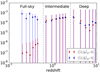 |
Fig. 7. Departures from 1 of the directional average of the inverse geometric magnification ⟨μ−1(z)⟩d and of the inverse observable magnification |

First of all, we note that we do not recover exactly ⟨μ−1(z)⟩d = 1, which yet should be exactly satisfied. For the full-sky cone (z < 0.5) the discrepancy is extremely small ( < 10−6) and is attributed to the discretisation of the full-sky map: averages are performed over a large but finite number of points. This interpretation is supported by the fact that ⟨μ−1(z < 0.5)⟩d is consistent with unity within the Poisson uncertainty. For the two other cones (z > 0.5), the discrepancy is larger ( ∼ 10−4). This should not come as a surprise, because ⟨μ−1⟩d = 1 is exact on the full sky only. The intermediate and deep narrow cones are simply slightly under-dense or over-dense with respect to the average box. Again, this interpretation is supported by the fact that ⟨μ−1(z)⟩d − 1 falls well into the error bars accounting for super-sample variance.
The direction-averaged inverse amplification  departs from 1 by almost 10−3 even for the full-sky data. We may note that, unlike μ,
  is subject to super-sample variance even on a full sky; however, the main reason for which
  at low z is the shift effect due to peculiar velocities (see Sect. 2.2.3). For the other two cones
  is mostly due to the super-sample variance as the one affecting ⟨μ−1(z)⟩d − 1.
Our results show that the approximation  is accurate up to 10−3 up to z = 10. They also indicate that incomplete sky coverage in actual observations may in the end be the main cause of any departure from
  at high redshift.
We now turn to the bias of angular or luminosity distance. For directional averaging, we expect d(z) to be negatively biased according to ⟨d(z)⟩d ≈ 1 − ⟨κ2(z)⟩/2. We evaluate ⟨κ2⟩ from the data directly as ⟨κ2⟩d, and we have checked that a pure-theory estimate based on the matter power spectrum gives the same results. As shown in Fig. 8, that theoretical prediction is in good agreement with numerical results within the error bars dominated by super-sample variance. Again, low-redshift departures are due to peculiar velocities whose shift effect is not accounted for in κ2. While ⟨μ−1(z)⟩d and  remains unity within error bars, ⟨d(z)⟩d − 1 clearly departs from zero for z > 1.
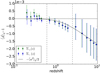 |
Fig. 8. Bias on the distance-redshift relation when averaged over directions, compared with the theoretical prediction ⟨d(z)⟩d = 1 − ⟨κ2(z)⟩/2. Since the iso-z surface is not unique, we indicated results for the closest surface Σ−(z) and farthest surface Σ+(z) from the observer. Expressions for the error bars may be found in Appedix D.1. |
We finally evaluate the accuracy of the expansion that allowed us to express all distance biases in terms of ⟨κ2(z)⟩ in Sect. 2.4. We shall take the direction-averaged magnification in order to illustrate that point. Taylor-expanding μ at order n in μ−1 − 1 yields
![Mathematical equation: $$ \begin{aligned} \mu = \left[1-(1-\mu ^{-1})\right]^{-1} = \underbrace{ \sum _{k=0}^n (1-\mu ^{-1})^k }_{\mu _{(n)}} + \mathcal{O} (1-\mu ^{-1})^{n+1}. \end{aligned} $$](/articles/aa/full_html/2021/11/aa40140-20/aa40140-20-eq156.gif) (67)
(67)
Figure 9 confronts ⟨μ⟩d with its Taylor-expansion ⟨μ(n)⟩d for n = 2, 3, 4, where all these quantities are evaluated numerically. The error bars only allow for Poisson errors, because super-sample variance affects μ and μ(n) in the same way. We see that the quadratic expansion ⟨μ(2)⟩d provides a good approximation of the exact result for z < 1. Beyond that, we observe discrepancies reaching about 10% at z = 10. These are due to departures from the weak-lensing regime (|μ−1 − 1|≪1), which are more likely to happen as the redshift increases. Figure 9 also illustrates the convergence of the series expansion of Eq. (67).
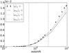 |
Fig. 9. Accuracy of the second-order expansion for the direction-averaged magnification. The error bars are only due to Poisson variance. |
4.1.2. Source averaging
We now analyse the mock halo catalogues produced for the three light cones (full sky, intermediate narrow and deep narrow) as described in Sect. 3.6.2. We arrange the haloes in tomographic bins of width Δz = 0.08, 0.2 and 1.5 for the full sky, intermediate and deep light cones, respectively.
We have seen in Sect. 2.3.2 that the source-average of the geometric and observable magnifications are expected to be almost unity  12. Unlike directional averaging, departures from equality may be caused by the non-trivial clustering of sources in addition to the shift and tilt corrections responsible for
  . Numerical results for
  are depicted in Fig. 10. Again, error bars account for both Poisson and super-sample (cosmic variance) whose expressions are given in Appendix D.1. Since the number of mock haloes per bin is smaller than the number of pixels of the maps used in Sect. 4.1.1, Poisson variance is larger here, especially at high redshift where it exceeds super-sample variance.
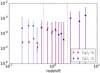 |
Fig. 10. Departures from 1 of the source-average of the geometric magnification ⟨μ(z)⟩s and of the observable magnification |

For the full-sky data (z < 0.5), we observe that |⟨μ(z)⟩s − 1|≈10−5, which is about 100 times larger than what was found for |⟨μ−1(z)⟩d − 1|. This discrepancy, which goes beyond the estimated uncertainty, is due to the fact that the latter does not properly account for the spatial clustering of haloes. Halo clustering is present in the d2N/d2θ kernel in the definition (22) of source averaging. The correlation between spatial clustering and lensing convergence was predicted to be on the order of 10−5 in Fleury et al. (2017a), Fanizza et al. (2020), which agrees with the present results. As for  , just as in Fig. 7 the numerical results are in agreement with unity within the error bars dominated by peculiar velocities.
The interpretation of the results for the intermediate (0.5 < z < 2) cone is similar to the directional-averaging case. The relative effect of the shift, that is, the main difference between μ and  , reduces as the impact of super-sample variance increases. As for the deep cone, Poisson variance dominates due to the small number of haloes per tomographic bin. In both cases, ⟨μ⟩s and
  are compatible with unity within error bars, so that no unexpected bias arises.
We now turn to more observationally relevant biases. For SN surveys, the common practice consists in fitting the magnitude-redshift relation m(z) with the FLRW prediction (Scolnic et al. 2018). Such a method is thus biased by ⟨Δm(z)⟩s = 5⟨log10d(z)⟩s. For standard-siren Hubble diagrams, it may be more common to fit the luminosity distance-redshift relation, which would be biased by ⟨d(z)⟩s. Numerical results on these biases are reported in Fig. 11, and compared with the theoretical predictions presented in Sect. 2.4. Similarly to Sect. 4.1.1, we estimate the variance of the convergence from the data itself. We note that ⟨κ2(z)⟩s slightly differs from ⟨κ2(z)⟩d; their relation is essentially given by Eq. (24).
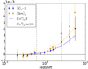 |
Fig. 11. Bias of the source-averaged distance-redshift ⟨d(z)⟩s (blue) and magnitude-redshift ⟨m(z)⟩s (yellow) relations. The associated solid lines are the theoretical predictions for these quantities as presented in Sect. 2.4. Error bars account for Poisson and super-sample variance; their expressions can be found in Appendix D.1. |
Again, our results agree with theoretical predictions within the error bars. We note that ⟨d(z)⟩s reaches a few 10−3 at high redshift, which may become non-negligible for the standard-siren Hubble diagrams of the future LISA mission (Caprini & Tamanini 2016). Such a bias would be easily removed by fitting  instead of DL(z), as pointed out by Fleury et al. (2017a).
We finally mention that, since d and m are non-linear functions of μ, theoretical predictions on their bias based on a second-order Taylor expansion are subject to the same small inaccuracies as displayed in Fig. 9. These inaccuracies are however much smaller than the uncertainty on those quantities, and hence may be safely neglected.
4.2. Focus on the shift correction
In Sect. 4.1, we have analysed the statistical biases to distance measures for both directional and source averaging. In particular, we have found no unexpected violation of  within numerical uncertainties. As seen in Sect. 2.5, this relation may be understood in terms of the area of iso-z surfaces, namely
  – the area is unaffected by inhomogeneities.
We now propose to further focus on the two subtle corrections that are making the above ‘≈’ differ from equality, namely the shift and tilt effects (see Fig. 1). We start, in the sub-section, with the analysis of the shift, that is, the discrepancy between the mean radius of a given light-cone slice (such as iso-z or iso-η) and its value in the FLRW background.
4.2.1. Wiggly ray effect: Mean distance reached at fixed distance travelled
We first consider the mean comoving distance that is reached by a photon after it travelled over a given comoving distance. As briefly described in Sect. 2.5.3, because light rays do not travel in straight lines, the radius reached for a distance travelled s is shorter than  . We may thus write
  , where δrgeo encodes this wiggly-ray effect. This is illustrated with a HEALPIX map of
  at z = 0.2 in Fig. 12. We see that the fluctuations are very small, on the order of 10−8, and vary on relatively small angular scales.
 |
Fig. 12. Map of wiggly-ray effect, that is, the relative fluctuations of the comoving distance reached at fixed distance travelled, |

On average, the wiggly-ray correction is found to read (see Appendix C.1.2)
 (68)
(68)
It may be noted, however, that Eq. (68) was obtained with the help of a few approximations, among which is Limber’s. A slightly more accurate computation, in the spirit of Eq. (A.26) in KP16, would yield
 (69)
(69)
with g(r)≡D+(η0 − r)/a(η0 − r) where D+ is the linear growth factor, ξϕ is the two-point correlation function of the gravitational potential at z = 0, and  is its derivative.
These theoretical predictions are successfully confronted with numerical results in Fig. 13. Error bars allow for both Poisson and correlated variance, whose expression is given in Appendix D.2. We note that the predictions of Eqs. (68) and (69) are very similar, but only the latter falls within error bars for the full-sky (z < 0.5) and intermediate cones (0.5 < z < 2).
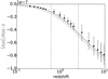 |
Fig. 13. Wiggly ray effect: Mean fractional reduction |

4.2.2. Shapiro effect: Mean distance reached at fixed time
We now investigate the mean comoving distance reached at constant time ⟨r(η)⟩; in other words, we consider the shift of iso-η surfaces, which would be relevant for CMB-like observations. A HEALPIX map of  is given in Fig. 14 for illustration. Compared to Fig. 12, we note that fluctuations are much larger (of order 10−4) and take place on much larger angular scales.
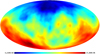 |
Fig. 14. Map of the relative fluctuations of the comoving distance reached at fixed time, |

As discussed in Sect. 2.5.3, in theory this shift may be decomposed in two components: (i) the wiggly-ray effect δrgeo considered above; and (ii) the Shapiro time-delay effect. The latter indeed changes the comoving distance travelled s(η) during a given time, compared to its background counterpart  , depending on the path-integrated gravitational potential experienced by light. Summarising,
 (70)
(70)
and as shown in Appendix C we expect
 (71)
(71)
because of the post-Born corrections to δs which turn out to be minus twice the geometrical contribution.
Numerical results are confronted with theory in Fig. 15. The first striking feature is perhaps that error bars are about two orders of magnitude larger than the ones of Fig. 13. This is because the time-delay contribution δs(η) is a first-order quantity, while δrgeo(η) is second-order. Thus, the corresponding super-sample variance is much larger. As such, the prediction (71) naturally falls in the error bars, which is not particularly informative.
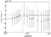 |
Fig. 15. Mean comoving distance reached at fixed time, ⟨r(η)⟩, compared to its background counterpart |


We may add an extra layer of refinement since we know the exact value of the gravitational potential in the simulation at the observer, ϕ0 ≈ −7 × 10⁻⁶ (which is about −2 km s−1). This information may be used to improve our prediction of δs(η) at low redshift. Precisely, following the method outlined in Sect. 3.11, we find that the average Shapiro contribution under the constraint ϕ(0) = ϕ0 totally overwhelms the geometrical and post-Born terms13, yielding
 (72)
(72)
The corresponding prediction is indicated by a solid line in Fig. 15, and is observed to reproduce the behaviour of numerical results at low redshift.
The fact that Fig. 15 is dominated by super-sample variance makes it a priori impossible to check the unconstrained prediction (71), which yet would be the most relevant at high redshift, where the effect of ϕ0 becomes negligible. However, we may apply the following trick to numerically extract the second-order contribution of ⟨δs(η)⟩. We consider the following estimator
 (73)
(73)
By construction, this combination eliminates the wiggly-ray and first-order Shapiro contributions to δr(η), while preserving the post-Born term of δs; see Appendix C.2.2 for details. Thus, we expect  . This is indeed roughly what is observed in Fig. 16, although the error bars seem to be under-estimated. This confirms our understanding of the subtle behaviour of r(η).
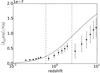 |
Fig. 16. Second-order (post-Born) contribution to δs(η). Dots indicate the numerical estimate from Eq. (73), while the solid line is the theoretical prediction −2⟨δrgeo(η)⟩. Error bars are twice those of Fig. 13. |
4.2.3. Doppler effect of peculiar velocities: Spatio-temporal shift at fixed observed redshift
We now turn to observations performed at fixed redshift z. In the inhomogeneous Universe, several phenomena may affect the observed redshift of a source at a given position: Doppler effect due to peculiar velocities, Sachs-Wolfe (SW) and ISW effects. These imply that for a given redshift, light may have been emitted slightly closer to the observer (and later), or slightly further (and earlier) compared to the background FLRW case. In other words, we have  and
and  , with δr = −δη the associated spatio-temporal shift of Σ(z).
The Doppler effect of peculiar velocities is expected to dominate, especially at low-z. Assuming that the observer is comoving (vo = 0), which is the case in the simulation, the shift due to the source’s peculiar velocity v reads
 (74)
(74)
at first order. We note that, combined with the (opposite) temporal shift, we find that the corresponding area perturbation reads ![Mathematical equation: $ \delta[a^2(\eta) r^2]/[a^2(\bar{\eta})\bar{r}^2]=2\tilde{\kappa}_{\mathit{v}} $](/articles/aa/full_html/2021/11/aa40140-20/aa40140-20-eq191.gif) , in agreement with Eq. (15).
, in agreement with Eq. (15).
Numerical results for ⟨δr(z)⟩d are shown in Fig. 17. Two values of δr(z) are provided for each z. This is because the fluctuations of peculiar velocities may be important on the light cone, so that several events may have the same redshift: Σ(z) is not unique. We plotted here the smallest one, ⟨minδr(z)⟩d, and the largest one, ⟨maxδr(z)⟩d. Numerical values for ⟨δr(z)⟩d account for all the redshift components at first order in metric perturbations; however, the super-sample variance contribution to the error bars only account for peculiar velocities, which are highly dominant. See Appendix D.3 for their expression.
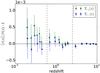 |
Fig. 17. Radial shift of surfaces of constant redshift. Dots indicate numerical results for |

The mean shift is compatible with zero within the large error bars, which is why we did not work on a more elaborate theoretical prediction for ⟨δr(z)⟩. We also note that the two extremal surfaces Σ−(z),Σ+(z) that we have considered differ more as we get closer to the observer. We shall now explain this point: at high redshift there are few virialised objects, and hence velocity dispersion is small next to such objects; thus, at high z, Σ(z) = Σ−(z) = Σ+(z) is typically unique. As z decreases, more haloes form, which implies that more regions have high velocity dispersion14, thereby de-multiplying Σ(z) and spreading its occurrences. The  factor in Eq. (74) further enhances that spread.
4.2.4. Affine parameter at constant time
While surfaces of constant redshift Σ(z) or time Σ(η) are observationally relevant, we may also consider surfaces of constant affine parameter Σ(λ), whose interest is strictly theoretical. Such light-cone slices have the advantage of being defined regardless of any specific model for the space-time metric. The analysis of Kibble & Lieu (2005) was indeed conducted on Σ(λ). We shall examine the time (or equivalently radial) shift at fixed affine parameter, δη(λ), in the next sub-section. Before that, we propose to first consider the converse shift δλ(η) for pedagogical reasons.
In the background FLRW model, the 0th component of the geodesic Eq. (2) is integrated as
 (75)
(75)
In the presence of perturbations, this becomes
![Mathematical equation: $$ \begin{aligned} \lambda (\eta ) = \int _{\eta }^{\eta _0} \mathrm{d} \eta^\prime \; a^2(\eta^\prime ) \left[1+2(\phi -\phi _0) - 2\int _0^{\eta^\prime } \mathrm{d} \eta^{\prime \prime }\; \frac{\partial \phi }{\partial \eta^{\prime \prime }}\right]\cdot \end{aligned} $$](/articles/aa/full_html/2021/11/aa40140-20/aa40140-20-eq195.gif) (76)
(76)
at first order (higher-order terms are negligible here). We note that since ⟨ϕ⟩ = 0, the mean correction to the affine parameter is simply  . However, we may account for the fact that, in our simulation just as in observations, the gravitational potential at the observer is fixed, and estimate ⟨δλ(η)⟩d with the following constrained ensemble average
![Mathematical equation: $$ \begin{aligned} \langle {\delta \lambda (\eta )|\phi _0}\rangle = -2\phi _0\int _0^{\bar{r}(\eta )} \mathrm{d} r \; a^2(\eta _0-r)\left[1-\frac{\xi _\phi (r)}{\xi _\phi (0)}\right] \not = 0, \end{aligned} $$](/articles/aa/full_html/2021/11/aa40140-20/aa40140-20-eq197.gif) (77)
(77)
where we chose to neglect the small ISW term of Eq. (76). In the high-z limit, this result may be approximated as
 (78)
(78)
with
 (79)
(79)
As shown in Fig. 18, the numerical results do follow the theoretical prediction of Eq. (77) within the error bars, although the unconstrained prediction  at first order would also be validated by the data. In particular,
  is indeed observed to converge to a constant at high z. For the deep cone (z > 2) the error bars are dominated by super-sample variance, but it seems that by chance the mean gravitational potential in these 400 deg2 is very close to zero.
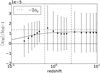 |
Fig. 18. Perturbation of the affine parameter at fixed time η. Dots are numerical results obtained by directional averaging; the solid line indicates the theoretical prediction (77); the dashed line shows −2ϕ0. Hence, the fractional difference between the dashed line and the asymptote of the solid line indicates Ξ∞. Error bars account for Poisson variance and constrained super-sample variance; see Appendix D.4 for details. |
We stress that error bars of Fig. 18 were computed in configuration space to account for the constraint ϕ(0) = ϕ0 on the variance (see Appendix D.4). For comparison, we also computed the variance in harmonic space using Eq. (63). Results were similar for the intermediate and deep cones, while for the full-sky cone the unconstrained error bars were twice larger than the constrained one. Had we disposed of full-sky data up to z = 10, the error bars at high-z would have been smaller than the bias of ⟨λ(η)⟩. In other words, ⟨δλ(η)⟩ = 0 would have been excluded.
4.2.5. Spatio-temporal shift at constant affine parameter
We now consider the time and radial shifts δη(λ) = − δr(λ) at fixed affine parameter, which is the converse of the above. For that operation, one would typically adopt a linearised approach and write  . However, since
  , this derivative can become quite large as the redshift increases, so that δλ may actually get out of the linear behaviour of
  . We may thus adopt a more accurate inversion that could be extrapolated up to the LSS. Specifically, we use
![Mathematical equation: $$ \begin{aligned} \eta (\lambda )&= \bar{\eta }\left\{ \bar{\lambda }[\eta (\lambda )]\right\} , \end{aligned} $$](/articles/aa/full_html/2021/11/aa40140-20/aa40140-20-eq205.gif) (80)
(80)
![Mathematical equation: $$ \begin{aligned}&= \bar{\eta }\left\{ \lambda [\eta (\lambda )]-\delta \lambda [\eta (\lambda )]\right\} , \end{aligned} $$](/articles/aa/full_html/2021/11/aa40140-20/aa40140-20-eq206.gif) (81)
(81)
![Mathematical equation: $$ \begin{aligned}&\approx \bar{\eta }\left\{ \lambda -\delta \lambda [\bar{\eta }(\lambda )]\right\} , \end{aligned} $$](/articles/aa/full_html/2021/11/aa40140-20/aa40140-20-eq207.gif) (82)
(82)
which we shall refrain from further expanding.
We have checked numerically that the fluctuations of λ(η) about its mean are much smaller than its bias ⟨δλ(η)⟩. This allows us to express the average emission time at λ as
![Mathematical equation: $$ \begin{aligned} \langle {\eta (\lambda )}\rangle \approx \bar{\eta }\left\{ \lambda -\langle {\delta \lambda [\bar{\eta }(\lambda )]}\rangle \right\} \equiv \bar{\eta }(\lambda )+\langle {\delta \eta (\lambda )}\rangle , \end{aligned} $$](/articles/aa/full_html/2021/11/aa40140-20/aa40140-20-eq208.gif) (83)
(83)
where ⟨δλ⟩ is given by Eq. (77).
As shown in Fig. 19, the prediction (83) interpreted as a radial shift ⟨δr(λ)⟩= − ⟨δη(λ)⟩ is in excellent agreement with the simulation data ⟨δr(λ)⟩d, although again 0 remains within the error bars dominated by super-sample variance at high-z. As expected, the amplitude of the shift blows up as λ increases.
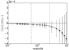 |
Fig. 19. Radial (or equivalently temporal) shift ⟨δr(λ)⟩= − ⟨δη(λ)⟩ at fixed affine parameter λ. Dots indicate numercal results from directional averaging; the solid line shows the theoretical prediction (83), while the dashed line indicates |
![Mathematical equation: $ \bar{r}[(1-2\phi_0)\lambda]-\bar{r}(\lambda) $](/articles/aa/full_html/2021/11/aa40140-20/aa40140-20-eq209.gif)
In fact, a linear expansion of Eq. (77) would also match our numerical results, whose redshift range is not large enough for the non-linear prescription to be critical. However, it does matter for the surface λ = λ*, that is the surface of constant affine parameter dictated by the background affine parameter of the LSS. In that case the linearised version of Eq. (77) would highly over-estimate the mean shift, which is already very large,  with ϕ0 = −2 km s−1 of our simulation.
We now need to investigate the consequences of such a large shift on the area A(λ*) of the surface of affine parameter λ*. Just as for iso-z surfaces, the time and radial shifts of iso-λ surfaces both contribute to the perturbation of their area, or equivalently to  . Accounting for that shift only (the tilt being second-order, it would be sub-dominant), we have
![Mathematical equation: $$ \begin{aligned} \frac{\delta A(\lambda _*)}{\bar{A}(\lambda _*)} = \left\langle {\frac{\delta \left\{ a^2[\eta (\lambda _*)] r^2(\lambda _*)\right\} }{a^2[\bar{\eta }(\lambda _*)]\bar{r}^2(\lambda _*)}}\right\rangle \approx \frac{a^2[\langle {\eta (\lambda _*)}\rangle ] -a^2[\bar{\eta }(\lambda _*)]}{a^2[\bar{\eta }(\lambda _*)]}, \end{aligned} $$](/articles/aa/full_html/2021/11/aa40140-20/aa40140-20-eq212.gif) (84)
(84)
which is dominated by the difference in scale factor15. Again, we shall refrain from linearising Eq. (84) because the time shift is large enough to invalidate a first-order Taylor expansion of a(η).
We illustrate the behaviour of Eq. (84) in Fig. 20 (black solid line) as a function of the observer’s potential. Even for reasonable values of that quantity, such as ϕ0 ∼ −10 km s−1, which is the order of magnitude expected within galaxy clusters (Wojtak et al. 2011, 2015), we find an astonishing δA(λ*)/ . We note that the black solid line of Fig. 20 is only plotted for negative values of ϕ0. This is because for ϕ0 > 0, ⟨δη(λ*)⟩< 0 quickly diverges as ϕ0 increases; since
  , it may not even be defined.
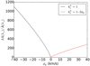 |
Fig. 20. Fractional change of the area A(λ*) of the surface of constant affine parameter λ = λ*, as a function of the gravitational potential ϕ0 at the observer. The black and red lines correspond to two different normalisations for the affine parameter. |
At that point, we may note that the affine parameter is defined up to an arbitrary normalisation. Here, this normalisation has been chosen so that  at the observer, hence λ coincides with cosmic time at that point. Another sensible choice consists in setting the observed frequency to unity,
  . This corresponds to a re-normalisation λ ↦ λ′ = (1 + 2ϕ0)λ, where now λ′ represents proper time at the observer. This alternative normalisation eliminates the ϕ0 term in Eq. (76) and yields
  instead of Eq. (78). However, the bias on the area
  remains huge, as seen with the red line of Fig. 2016, which corresponds to that alternative normalisation for the affine parameter. The only way to avoid such a huge bias would be to define λ″ with the quite un-natural normalisation
  .
.
The perhaps surprising results reported in this section must be attributed to the fact that  when η → −∞, so that
  flattens out and saturates in the early Universe. This makes η extremely sensitive to even tiny changes in λ. All in all, this indicates that the affine parameter is a rather dangerous quantity to be used in theoretical analyses of light propagation down to the early Universe. The huge bias on A(λ) shown in Fig. 20 must be considered a theoretical hiccup with no observational consequences.
4.3. Focus on the tilt correction
We may close this section on numerical results by evaluating the tilt, or wrinkly-surface effect, which tends to increase the inverse amplification  and the area of light-cone slices. As outlined in Sect. 2.2.3 and illustrated in Fig. 1, the tilt is defined as the angle ι between the radial direction β of a point and the local direction of light propagation at that point.
The contribution of the tilt to the area A(p) of an iso-p surface, or equivalently to the directional average of the inverse amplification  , where p is any relevant parameter, goes as ι2(p); it is always a second-order quantity. As such, it does not matter much which parameter p is actually considered here. Indeed, for any two parameters p, q (which can stand for z, η, λ, …) we have ι(p)/ι(q)−1 ∼ |shift(p)−shift(q)| ≪ 1. In other words, the tilt can be considered universal in first approximation.
In light of the above discussion, we shall consider the tilt over surfaces of constant time, keeping in mind that the result would equally apply to other ways to slice the light cone. The choice of iso-η surfaces is also motivated by the fact that, in this case17, ι coincides with the angle formed by the normal n to the surface and the radial direction β, as seen in Sect. 2.5.3. Thus,
![Mathematical equation: $$ \begin{aligned} \cos \iota (\eta ,\boldsymbol{\beta }) = \boldsymbol{\beta }\cdot \boldsymbol{n}(\eta ,\boldsymbol{\beta }) = \left[1 + \left| \frac{1}{r(\eta ,\boldsymbol{\beta })} \frac{\partial r}{\partial \boldsymbol{\beta }} \right|^2 \right]^{-1/2}\cdot \end{aligned} $$](/articles/aa/full_html/2021/11/aa40140-20/aa40140-20-eq224.gif) (85)
(85)
At second order, the area increase due to the tilt is predicted to be (see Appendix C.4 for details),
 (86)
(86)
with J(r) given in Eq. (49).
This prediction is successfully confronted with numerical results following Sect. 3.8 in Fig. 21. This ends our series of numerical checks of the remarkably accurate predictions of KP16.
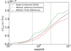 |
Fig. 21. Wrinkly-surface effect: relative increase of the area of surfaces of constant time due to their non-sphericity. The black solid line indicates the theoretical prediction (86) as originally found by KP16. The green and red lines indicate numerical results obtained from the two different methods outlined in Sect. 3.8. |
5. Conclusion
The general topic of this article was the effect of inhomogeneities on cosmological observables, notably the average result of cosmic distance measurements. In the theoretical part (Sect. 2), we started by emphasising the subtle difference between the notions of geometric magnification μ and observable magnification  . We interpreted that difference in terms of shifts and tilts associated with light propagation in the inhomogeneous Universe. We then reviewed and compared various notions of averaging involved in cosmology, in particular directional averaging ⟨⋯⟩d and source-averaging ⟨⋯⟩s.
We argued that, because of the exact identity ⟨μ−1⟩d = 1, one may expect the approximate relations  . Departures from the exact
  are due to the shift and tilt effects. We rigorously showed that such statements may be reformulated in terms of the area A of slices of the light cone; namely A should be almost unaffected by cosmological inhomogeneities, which is the conjecture of Weinberg (1976). Finally, we have reviewed how
  allows one to predict the statistical bias of any distance measure, such as the magnitude in SN surveys.
Most of the above theoretical considerations had been investigated in the past, notably in KP16, within the framework of cosmological perturbation theory at second order. The main addition of this article is their thorough analysis via ray tracing in a high-resolution N-body simulation up to z = 10. This tool (Sect. 3) allowed us to account for the inhomogeneity of the Universe down to very small scales, where the perturbation theory fails. We produced HEALPIX maps and halo catalogues to generate direction-averaged and source-averaged mock observations respectively. Our main results are the following:
-
(i)
At all redshifts, we confirmed that
 within our error bars, which account for both Poisson and super-sample variance. Source-averaged quantities were found to be more biased due to real-space clustering.
 -
(ii)
Still within error bars, the bias on the direction-averaged distance is ⟨δd(z)⟩d = −⟨κ2⟩/2, while the source-averaged distance and distance modulus are biased as ⟨δd(z)⟩s = 3⟨κ2⟩/2 and ⟨Δm(z)⟩s = 5⟨κ2⟩/ln10. All these numerical results thus agree very well (within error bars) with theoretical predictions. A large scatter is observed at low redshift due to peculiar velocities.
-
(iii)
In order to further test the accuracy of Weinberg’s conjecture, we investigated in detail the discrepancy between geometric and observable magnifications
 , that is, the effects of shift and tilt. We found that the fractional area perturbations of Σ(η) are well recovered by the predictions of KP16, of the order of order 10−7. However, this bias turned out to be much smaller than the super-sample variance on time delays, which is on the order of 10−5. Furthermore, we checked that propagating light rays on a coarse grid (rather than the AMR grid) does not impact the discrepancy between μ and
  , which shows that the latter is relatively insensitive to very small scales.
Summarising, our results show no unexpectedly large bias for source and direction-averaged observables. They also confirm Weinberg’s conjecture that the area of surfaces of constant redshift, or constant time, are almost unaffected by inhomogeneities, with corrections remaining below a part in a million for the latter (while the former might be slightly larger at low z due to peculiar velocities, but so is the associated variance).
As a theoretical curiosity, we also considered the area bias of surfaces of constant affine parameter, Σ(λ). We found that at very high redshift, the bias grows quickly and eventually diverges, because η ↦ λ(η) reaches a flat asymptote for η → −∞. In practice, this leads to absurdly large corrections to A(λ), and shows that one should avoid the use of the affine parameter to describe light rays in the early Universe.
For the present analysis we used finite ray bundles to compute the lensing distortion matrix 𝒜. This allowed us, as a side product, to test the predictions of the finite-beam formalism developed by Fleury et al. (2017b, 2019a,b). Specifically, we checked that the convergence and shear power spectrum for finite ray bundles were suppressed for scales smaller than the bundle’s width, in excellent agreement with Fleury et al. (2019a). Last, we found that treating the gravitational potential field ϕ as a constrained field near the observer, improves the agreement between numerical data and theoretical predictions.
Several extensions are possibles for this work: at very large scale it could be interesting to see the impact of a fully general relativistic treatment, either by correcting the results from a Newtonian N-body code (Chisari & Zaldarriaga 2011; Fidler et al. 2015) or by directly using GR simulations (Adamek et al. 2016; Barrera-Hinojosa & Li 2020). At smaller scales, one could investigate the effect of strong lensing, allowing for multiple images for a single source. Also, we studied the bias on the distance-redshift relation within the ΛCDM framework. One could perform a similar analysis using different cosmologies, for example by changing the nature of the dark sector or departing from GR, to see how such new physics may be degenerate with observational biases.
This talk was mentioned in the introduction of Gunn (1967).
In a more modern language, we may say that the calculation was made at first order in the micro-lensing optical depth τ, which coincides with the convergence κ if the density of the lenses were smoothed out; see, for instance, Sect. II.C of Fleury & García-Bellido (2020).
In fact, Eq. (15) not only allows for the shift of the iso-z surface, but also for the optical aberration effect due to the observer’s velocity. If the observer moves towards the source ( ), then the source appears smaller to them,
  .
.
This approximation fails at low-z, where peculiar velocities generate Malmquist bias (Ben-Dayan et al. 2014; Kaiser & Hudson 2015).
The natural frame is not unique; there is in fact a class of natural frames which are all related by Lorentz boosts in the local direction of light propagation. The area of d2x is invariant under such boosts, as long as they go from one natural frame to another one.
This is of course a gauge-dependent statement, see for example Ellis & Durrer (2018) for a discussion.
In KP16 that same quantity is denoted λ. We adopt s instead in order to avoid confusions with the affine parameter.
We have also implemented another prescription where the screen is orthogonal to the photon direction.
This formalism was initially developed to tackle the Ricci-Weyl paradox in the gravitational-lensing theory. It was later applied to determining the effect of the finite size of light sources in weak-lensing surveys.
The total number of pixels in a full-sky HEALPIX map is given by Npix = 12 × nside2.
The halo catalogues, as well as convergence and magnification HEALPIX maps are available at http://cosmo.obspm.fr/raygalgroupsims-relativistic-halo-catalogs
In principle these (approximate) relations should apply to the total absolute magnification rather than to the signed magnification. As mentioned in Sect. 2.3, they coincide in the absence of multiple imaging, which is a good approximation here. In fact, no negative-parity image was found in our halo catalogue. This is mostly due to the source-averaging procedure, which is expected to give less strong-lensing events that the directional averaging one, coupled with the fact that there are less sources at high redshift. Another reason is the use of ray bundles, which tend to smooth out the matter inhomogeneities on very small scales and thereby reduce the occurrence of strong lensing.
This finding does not contradict the conclusions of Hall (2020) that the impact of our local gravitational potential is negligible in current weak-lensing and galaxy-clustering surveys, because they concern very different cosmological quantities.
This is known as the Finger-of-God effect in galaxy clustering and redshift-space distortions analysis.
This is because the surface λ = λ* is very far from the observer. For closer surfaces the radial shift would dominate.
This red line is only plotted for ϕ0 ≥ 0 for the same reason as the black line is only plotted for ϕ0 ≤ 0. Namely,  quickly diverges and may not even exist when ϕ0 < 0.
This property would apply to other surfaces in their natural frame, which is not necessarily the comoving frame.
Anisotropic emission would bring additional effects that go beyond the problematic of this article.
The cautious reader may note that our definition of δrgeo differs from (A21) of KP16. Specifically, our approach involves the angle ι between the photon direction and β, while KP16 consider instead the angle between photon propagation and the instantaneous photon position β + ξ(r)/r. Our methods yield the same final result for δrgeo.
Acknowledgments
This paper is the continuation of a work that started during Vincent Reverdy’s PhD thesis (Reverdy 2014). MAB thanks Sylvain de la Torre for pointing out the paper of Desjacques et al. (2021). We thank the referee John Peacock for many relevant comments which significantly improved the quality of this manuscript, especially in Sect. 2. This work was granted access to HPC resources of TGCC through allocations made by GENCI (Grand Equipement National de Calcul Intensif) under the allocations A0050402287 and A0070402287. PF received the support of a fellowship from “la Caixa” Foundation (ID 100010434). The fellowship code is LCF/BQ/PI19/11690018.
References
- Abbott, T., Allam, S., Andersen, P., et al. 2019, ApJ, 872, L30 [NASA ADS] [CrossRef] [Google Scholar]
- Adamek, J., Daverio, D., Durrer, R., & Kunz, M. 2016, JCAP, 7, 053 [CrossRef] [Google Scholar]
- Adamek, J., Clarkson, C., Coates, L., Durrer, R., & Kunz, M. 2019, Phys. Rev. D, 100, 021301 [NASA ADS] [CrossRef] [Google Scholar]
- Alam, S., Aubert, M., Avila, S., et al. 2021, Phys. Rev. D, 103, 083533 [NASA ADS] [CrossRef] [Google Scholar]
- Bacon, D. J., Andrianomena, S., Clarkson, C., Bolejko, K., & Maartens, R. 2014, MNRAS, 443, 1900 [NASA ADS] [CrossRef] [Google Scholar]
- Bagla, J. S., & Ray, S. 2005, MNRAS, 358, 1076 [CrossRef] [Google Scholar]
- Bardeen, J. M. 1980, Phys. Rev. D, 22, 1882 [NASA ADS] [CrossRef] [Google Scholar]
- Barreira, A., Llinares, C., Bose, S., & Li, B. 2016, JCAP, 5, 001 [NASA ADS] [Google Scholar]
- Barrera-Hinojosa, C., & Li, B. 2020, JCAP, 01, 007 [CrossRef] [Google Scholar]
- Ben-Dayan, I., Marozzi, G., Nugier, F., & Veneziano, G. 2012, JCAP, 11, 045 [CrossRef] [Google Scholar]
- Ben-Dayan, I., Durrer, R., Marozzi, G., & Schwarz, D. J. 2014, Phys. Rev. Lett., 112, 221301 [NASA ADS] [CrossRef] [Google Scholar]
- Bentivegna, E., Korzyński, M., Hinder, I., & Gerlicher, D. 2017, JCAP, 03, 014 [CrossRef] [Google Scholar]
- Biswas, T., & Notari, A. 2008, JCAP, 0806, 021 [CrossRef] [Google Scholar]
- Blandford, R., & Narayan, R. 1986, ApJ, 310, 568 [Google Scholar]
- Bolejko, K. 2009, Gen. Rel. Grav., 41, 1737 [NASA ADS] [CrossRef] [Google Scholar]
- Bolejko, K. 2011, JCAP, 2, 25 [Google Scholar]
- Bolejko, K., & Célérier, M.-N. 2010, Phys. Rev. D, 82, 103510 [NASA ADS] [CrossRef] [Google Scholar]
- Bolejko, K., Clarkson, C., Maartens, R., et al. 2013, Phys. Rev. Lett., 110, 021302 [NASA ADS] [CrossRef] [Google Scholar]
- Bonvin, C. 2008, Phys. Rev. D, 78, 123530 [NASA ADS] [CrossRef] [Google Scholar]
- Bonvin, C., Durrer, R., & Gasparini, M. A. 2006, Phys. Rev. D, 73, 023523 [Google Scholar]
- Bonvin, C., Clarkson, C., Durrer, R., Maartens, R., & Umeh, O. 2015a, JCAP, 06, 050 [Google Scholar]
- Bonvin, C., Clarkson, C., Durrer, R., Maartens, R., & Umeh, O. 2015b, JCAP, 07, 040 [CrossRef] [Google Scholar]
- Breton, M.-A., Rasera, Y., Taruya, A., Lacombe, O., & Saga, S. 2019, MNRAS, 483, 2671 [NASA ADS] [CrossRef] [Google Scholar]
- Brouzakis, N., Tetradis, N., & Tzavara, E. 2007, JCAP, 2, 13 [Google Scholar]
- Brouzakis, N., Tetradis, N., & Tzavara, E. 2008, JCAP, 0804, 008 [NASA ADS] [Google Scholar]
- Bruneton, J.-P., & Larena, J. 2013, Class. Quant. Grav., 30, 025002 [NASA ADS] [CrossRef] [Google Scholar]
- Burke, W. L. 1981, ApJ, 244, L1 [NASA ADS] [CrossRef] [Google Scholar]
- Caprini, C., & Tamanini, N. 2016, JCAP, 10, 006 [Google Scholar]
- Chisari, N. E., & Zaldarriaga, M. 2011, Phys. Rev. D, 83, 123505 [NASA ADS] [CrossRef] [Google Scholar]
- Chon, G., Challinor, A., Prunet, S., Hivon, E., & Szapudi, I. 2004, MNRAS, 350, 914 [Google Scholar]
- Clarkson, C., Umeh, O., Maartens, R., & Durrer, R. 2014, JCAP, 11, 036 [Google Scholar]
- Clifton, T., & Ferreira, P. G. 2009a, Phys. Rev. D, 80, 103503 [NASA ADS] [CrossRef] [Google Scholar]
- Clifton, T., & Ferreira, P. G. 2009b, JCAP, 10, 026 [Google Scholar]
- Clifton, T., & Ferreira, P. G. 2011, Phys. Rev. D, 84, 109902 [NASA ADS] [CrossRef] [Google Scholar]
- Clifton, T., & Zuntz, J. 2009, MNRAS, 400, 2185 [NASA ADS] [CrossRef] [Google Scholar]
- Clifton, T., Ferreira, P. G., & O’Donnell, K. 2012, Phys. Rev. D, 85, 023502 [NASA ADS] [CrossRef] [Google Scholar]
- Corasaniti, P. S., Ettori, S., Rasera, Y., et al. 2018, ApJ, 862, 40 [CrossRef] [Google Scholar]
- Dashevskii, V. M., & Slysh, V. I. 1966, Sov. Astron., 9, 671 [NASA ADS] [Google Scholar]
- Davis, T. M., Hui, L., Frieman, J. A., et al. 2011, ApJ, 741, 67 [NASA ADS] [CrossRef] [Google Scholar]
- Desjacques, V., Ginat, Y. B., & Reischke, R. 2021, MNRAS, 504, 5612 [NASA ADS] [CrossRef] [Google Scholar]
- Di Dio, E., Vonlanthen, M., & Durrer, R. 2012, JCAP, 02, 036 [CrossRef] [Google Scholar]
- Dyer, C. C., & Roeder, R. C. 1974, ApJ, 189, 167 [CrossRef] [Google Scholar]
- Ellis, G. F. R., & Durrer, R. 2018, ArXiv e-prints [arXiv:1806.09530] [Google Scholar]
- Ellis, G. F. R., Bassett, B. A. C. C., & Dunsby, P. K. S. 1998, Class. Quant. Grav., 15, 2345 [NASA ADS] [CrossRef] [Google Scholar]
- Etherington, I. M. H. 1933, Phil. Mag., 15, 761 [NASA ADS] [CrossRef] [Google Scholar]
- Fanizza, G., Gasperini, M., Marozzi, G., & Veneziano, G. 2020, JCAP, 02, 017 [Google Scholar]
- Fidler, C., Rampf, C., Tram, T., et al. 2015, Phys. Rev. D, 92, 123517 [NASA ADS] [CrossRef] [Google Scholar]
- Fidler, C., Tram, T., Rampf, C., et al. 2016, JCAP, 9, 031 [Google Scholar]
- Flanagan, E. E., Kumar, N., & Wasserman, I. 2013, Phys. Rev. D, 88, 043004 [NASA ADS] [CrossRef] [Google Scholar]
- Fleury, P. 2014, JCAP, 06, 054 [CrossRef] [Google Scholar]
- Fleury, P. 2015, PhD Thesis, Paris U., VI, IAP [Google Scholar]
- Fleury, P., & García-Bellido, J. 2020, Phys. Dark Univ., 29, 100567 [NASA ADS] [CrossRef] [Google Scholar]
- Fleury, P., Dupuy, H., & Uzan, J.-P. 2013, Phys. Rev. D, 87, 123526 [NASA ADS] [CrossRef] [Google Scholar]
- Fleury, P., Clarkson, C., & Maartens, R. 2017a, JCAP, 3, 062 [CrossRef] [Google Scholar]
- Fleury, P., Larena, J., & Uzan, J.-P. 2017b, Phys. Rev. Lett., 119, 191101 [NASA ADS] [CrossRef] [Google Scholar]
- Fleury, P., Larena, J., & Uzan, J.-P. 2019a, Phys. Rev. D, 99, 023525 [NASA ADS] [CrossRef] [Google Scholar]
- Fleury, P., Larena, J., & Uzan, J.-P. 2019b, Phys. Rev. D, 99, 023526 [NASA ADS] [CrossRef] [Google Scholar]
- Fluke, C. J., & Lasky, P. D. 2011, MNRAS, 416, 1616 [NASA ADS] [CrossRef] [Google Scholar]
- Fluke, C. J., Webster, R. L., & Mortlock, D. J. 1999, MNRAS, 306, 567 [NASA ADS] [CrossRef] [Google Scholar]
- Fosalba, P., Gaztañaga, E., Castander, F. J., & Manera, M. 2008, MNRAS, 391, 435 [NASA ADS] [CrossRef] [Google Scholar]
- Freedman, W. L., Madore, B. F., Hatt, D., et al. 2019, ApJ, 882, 34 [Google Scholar]
- Gelb, J. M., & Bertschinger, E. 1994, ApJ, 436, 491 [NASA ADS] [CrossRef] [Google Scholar]
- Giblin, J. T., Jr., Mertens, J. B., & Starkman, G. D. 2016, ApJ, 833, 247 [NASA ADS] [CrossRef] [Google Scholar]
- Górski, K. M., Hivon, E., Banday, A. J., et al. 2005, ApJ, 622, 759 [Google Scholar]
- Green, S. R., & Wald, R. M. 2014, Class. Quant. Grav., 31, 234003 [NASA ADS] [CrossRef] [Google Scholar]
- Guillet, T., & Teyssier, R. 2011, J. Comput. Phys., 230, 4756 [Google Scholar]
- Gunn, J. E. 1967, ApJ, 150, 737 [NASA ADS] [CrossRef] [Google Scholar]
- Hall, A. 2020, Phys. Rev. D, 101, 043519 [CrossRef] [Google Scholar]
- Harnois-Déraps, J., & van Waerbeke, L. 2015, MNRAS, 450, 2857 [Google Scholar]
- Helbig, P. 2020, Open J. Astrophys., 3, 1 [CrossRef] [Google Scholar]
- Hilbert, S., Hartlap, J., White, S. D. M., & Schneider, P. 2009, A&A, 499, 31 [NASA ADS] [CrossRef] [EDP Sciences] [Google Scholar]
- Hockney, R. W., & Eastwood, J. W. 1981, Computer Simulation Using Particles (New York: McGraw-Hill) [Google Scholar]
- Hoffman, Y., & Ribak, E. 1991, ApJ, 380, L5 [NASA ADS] [CrossRef] [Google Scholar]
- Holz, D. E., & Hughes, S. A. 2005, ApJ, 629, 15 [Google Scholar]
- Hui, L., & Greene, P. B. 2006, Phys. Rev. D, 73, 123526 [NASA ADS] [CrossRef] [Google Scholar]
- Jain, B., Seljak, U., & White, S. 2000, ApJ, 530, 547 [NASA ADS] [CrossRef] [Google Scholar]
- Kaiser, N. 1987, MNRAS, 227, 1 [Google Scholar]
- Kaiser, N., & Hudson, M. J. 2015, MNRAS, 454, 280 [Google Scholar]
- Kaiser, N., & Peacock, J. A. 2016, MNRAS, 455, 4518 [NASA ADS] [CrossRef] [Google Scholar]
- Kantowski, R. 1969, ApJ, 155, 89 [NASA ADS] [CrossRef] [Google Scholar]
- Kibble, T. W. B., & Lieu, R. 2005, ApJ, 632, 718 [NASA ADS] [CrossRef] [Google Scholar]
- Kilbinger, M., Heymans, C., Asgari, M., et al. 2017, MNRAS, 472, 2126 [Google Scholar]
- Koksbang, S. M. 2017, Phys. Rev. D, 95, 063532 [NASA ADS] [CrossRef] [Google Scholar]
- Koksbang, S. M. 2019a, Class. Quant. Grav., 36, 185004 [NASA ADS] [CrossRef] [Google Scholar]
- Koksbang, S. M. 2019b, Phys. Rev. D, 100, 063533 [NASA ADS] [CrossRef] [Google Scholar]
- Koksbang, S. 2020a, JCAP, 11, 061 [Google Scholar]
- Koksbang, S. M. 2020b, MNRAS, 498, L135 [NASA ADS] [CrossRef] [Google Scholar]
- Komatsu, E., Smith, K. M., Dunkley, J., et al. 2011, ApJS, 192, 18 [Google Scholar]
- Lavinto, M., & Rasanen, S. 2015, JCAP, 10, 057 [CrossRef] [Google Scholar]
- Lepori, F., Adamek, J., Durrer, R., Clarkson, C., & Coates, L. 2020, MNRAS, 497, 2078 [NASA ADS] [CrossRef] [Google Scholar]
- Lewis, A., Challinor, A., & Lasenby, A. 2000, ApJ, 538, 473 [Google Scholar]
- Liu, R. G. 2015, Phys. Rev. D, 92, 063529 [NASA ADS] [CrossRef] [Google Scholar]
- Marra, V., Kolb, E. W., & Matarrese, S. 2008, Phys. Rev. D, 77, 023003 [NASA ADS] [CrossRef] [Google Scholar]
- Mitsou, E., Yoo, J., Durrer, R., Scaccabarozzi, F., & Tansella, V. 2020, Phys. Rev. Res., 2, 033004 [CrossRef] [Google Scholar]
- Odderskov, I., Koksbang, S. M., & Hannestad, S. 2016, JCAP, 2, 001 [NASA ADS] [Google Scholar]
- Okamura, T., & Futamase, T. 2009, Prog. Theor. Phys., 122, 511 [CrossRef] [Google Scholar]
- Peel, A., Troxel, M. A., & Ishak, M. 2014, Phys. Rev. D, 90, 123536 [NASA ADS] [CrossRef] [Google Scholar]
- Pen, U.-L. 1997, ApJ, 490, L127 [NASA ADS] [CrossRef] [Google Scholar]
- Perlmutter, S., Aldering, G., della Valle, M., et al. 1998, Nature, 391, 51 [CrossRef] [Google Scholar]
- Peter, P., & Uzan, J.-P. 2013, Primordial Cosmology. Oxford Graduate Texts (Oxford: Oxford University Press) [Google Scholar]
- Planck Collaboration VI. 2020, A&A, 641, A6 [NASA ADS] [CrossRef] [EDP Sciences] [Google Scholar]
- Power, C., & Knebe, A. 2006, MNRAS, 370, 691 [NASA ADS] [Google Scholar]
- Prunet, S., Pichon, C., Aubert, D., et al. 2008, ApJS, 178, 179 [NASA ADS] [CrossRef] [Google Scholar]
- Reverdy, V. 2014, PhD Thesis, Laboratoire Univers et Théories [Google Scholar]
- Riess, A. G., Filippenko, A. V., Challis, P., et al. 1998, AJ, 116, 1009 [Google Scholar]
- Riess, A. G., Casertano, S., Yuan, W., Macri, L. M., & Scolnic, D. 2019, ApJ, 876, 85 [Google Scholar]
- Roy, F., Bouillot, V. R., & Rasera, Y. 2014, A&A, 564, A13 [NASA ADS] [CrossRef] [EDP Sciences] [Google Scholar]
- Sachs, R. 1961, Proc. R. Soc. London Ser. A, 264, 309 [NASA ADS] [CrossRef] [Google Scholar]
- Sanghai, V. A. A., Fleury, P., & Clifton, T. 2017, JCAP, 7, 028 [CrossRef] [Google Scholar]
- Sasaki, M. 1987, MNRAS, 228, 653 [Google Scholar]
- Schneider, P., Ehlers, J., & Falco, E. E. 1992, Gravitational Lenses (Berlin: Springer-Verlag) [Google Scholar]
- Scoccimarro, R. 1998, MNRAS, 299, 1097 [NASA ADS] [CrossRef] [Google Scholar]
- Scolnic, D. M., Jones, D. O., Rest, A., et al. 2018, ApJ, 859, 101 [NASA ADS] [CrossRef] [Google Scholar]
- Sheth, R. K., & Tormen, G. 1999, MNRAS, 308, 119 [Google Scholar]
- Sirko, E. 2005, ApJ, 634, 728 [NASA ADS] [CrossRef] [Google Scholar]
- Smith, R. E., Peacock, J. A., Jenkins, A., et al. 2003, MNRAS, 341, 1311 [Google Scholar]
- Szapudi, I., Prunet, S., Pogosyan, D., Szalay, A. S., & Bond, J. R. 2001, ApJ, 548, L115 [Google Scholar]
- Szybka, S. J. 2011, Phys. Rev. D, 84, 044011 [NASA ADS] [CrossRef] [Google Scholar]
- Takahashi, R., Sato, M., Nishimichi, T., Taruya, A., & Oguri, M. 2012, ApJ, 761, 152 [Google Scholar]
- Teyssier, R. 2002, A&A, 385, 337 [NASA ADS] [CrossRef] [EDP Sciences] [Google Scholar]
- Teyssier, R., Pires, S., Prunet, S., et al. 2009, A&A, 497, 335 [NASA ADS] [CrossRef] [EDP Sciences] [Google Scholar]
- Troxel, M. A., Ishak, M., & Peel, A. 2014, JCAP, 3, 40 [Google Scholar]
- Umeh, O., Clarkson, C., & Maartens, R. 2014, Class. Quant. Grav., 31, 202001 [CrossRef] [Google Scholar]
- Valkenburg, W. 2009, JCAP, 0906, 010 [Google Scholar]
- van de Weygaert, R., & Bertschinger, E. 1996, MNRAS, 281, 84 [NASA ADS] [CrossRef] [Google Scholar]
- Vanderveld, R. A., Flanagan, E. E., & Wasserman, I. 2008, Phys. Rev. D, 78, 083511 [CrossRef] [Google Scholar]
- Weinberg, S. 1976, ApJ, 208, L1 [NASA ADS] [CrossRef] [Google Scholar]
- Wojtak, R., Hansen, S. H., & Hjorth, J. 2011, Nature, 477, 567 [NASA ADS] [CrossRef] [Google Scholar]
- Wojtak, R., Davis, T. M., & Wiis, J. 2015, JCAP, 07, 025 [CrossRef] [Google Scholar]
- Wong, K. C., Suyu, S. H., Chen, G. C. F., et al. 2019, MNRAS, 498, 1420 [Google Scholar]
- Wucknitz, O. 2008, MNRAS, 386, 230 [NASA ADS] [CrossRef] [Google Scholar]
- Yoo, J., & Scaccabarozzi, F. 2016, JCAP, 9, 046 [CrossRef] [Google Scholar]
- Zel’dovich, Y. B. 1964, Sov. Astron., 8, 13 [Google Scholar]
- Zonca, A., Singer, L., Lenz, D., et al. 2019, J. Open Sour. Softw., 4, 1298 [Google Scholar]
Appendix A: Alternative approach to the shift and tilt corrections
In Sect. 2.2.3 we have presented the shift and tilt corrections to the magnification by assuming that the source was an infinitesimal element of the iso-z surface. This choice of formulation was justified by its tight connection with the subsequent considerations on the area of light-cone slices. Having said that, the curious reader may wonder about the generality of the shift and tilt corrections as defined therein. We may now consider an individual source instead of an element of iso-z surface. This appendix aims to show that the results of Sect. 2.2.3 equally applies to this case.
We assume, for simplicity, that the source at redshift z is spherical with isotropic emission18. Recall that the geometric and observational magnifications are respectively defined as
 (A.1)
(A.1)
 (A.2)
(A.2)
where d2θ is the angular size of an image, d2β the coordinate solid angle covered by the source, and  the apparent size of that source if it were placed at the same redshift in an FLRW universe (see Fig. A.1). The difference between μ and
  lies in the subtle difference between d2β and
  .
.
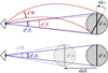 |
Fig. A.1. Illustration of the shift and tilt effects, implying that the observable magnification differs from the geometric magnification, in the case of an isotropic spherical source. |
Since the source is spherical, it is equivalent to a disk of area d2A orthogonal to the direction of light propagation at emission. However, due to light deflection, this disk is tilted with respect to the radial direction. As a consequence, the disk covers a smaller coordinate solid angle d2β than its non-tilted counterpart d2β⊥ (top of Fig. A.1). Both are related by d2β = d2β⊥ cos ι.
Besides, due to redshift corrections in the inhomogeneous Universe (peculiar velocities, Sachs-Wolfe effect, etc.) the time and radial coordinates of the source are shifted with respect to their background counterparts. As a result, a source with a given size is seen under a different solid angle in both cases (bottom of Fig. A.1), namely
![Mathematical equation: $$ \begin{aligned} \frac{\mathrm{d} ^2\bar{\boldsymbol{\theta }}}{\mathrm{d} ^2\boldsymbol{\beta }_\perp } = \frac{a^2[\eta (z)]\, r^2(z)}{a^2[\bar{\eta }(z)] \, \bar{r}^2(z)}\cdot \end{aligned} $$](/articles/aa/full_html/2021/11/aa40140-20/aa40140-20-eq241.gif) (A.3)
(A.3)
Summarising, the geometric and observational magnifications are related by
![Mathematical equation: $$ \begin{aligned} \frac{\tilde{\mu }(z, \boldsymbol{\theta })}{\mu (z, \boldsymbol{\theta })} = \frac{\mathrm{d} ^2\boldsymbol{\beta }}{\mathrm{d} ^2\bar{\boldsymbol{\theta }}} = \underbrace{\frac{\mathrm{d} ^2\boldsymbol{\beta }_\perp }{\mathrm{d} ^2\bar{\boldsymbol{\theta }}}}_{\mathrm{shift} } \underbrace{\frac{\mathrm{d} ^2\boldsymbol{\beta }}{\mathrm{d} ^2\boldsymbol{\beta }_\perp }}_{\mathrm{tilt} } = \frac{a^2[\bar{\eta }(z)] \, \bar{r}^2(z)}{a^2[\eta (z)]\, r^2(z)} \, \cos \iota , \end{aligned} $$](/articles/aa/full_html/2021/11/aa40140-20/aa40140-20-eq242.gif) (A.4)
(A.4)
which is indeed equivalent to Eq. (14).
Appendix B: Finite-beam corrections
In this appendix we derive the finite-beam corrections (52), (53) to the power spectra of convergence and shear. The computation will follow the general philosophy of Fleury et al. (2017b, 2019a,b), but it will differ in the details, due to the specific four-ray set-up used to compute κ and γ in this article.
B.1. Estimators of convergence and shear
As shown by Fleury et al. (2019a), finite-beam corrections to cosmic convergence and shear occur on very small scales. Thus, we can safely work in the flat-sky approximation in the following. In that context, the lens equation reads
 (B.1)
(B.1)
where β is the position of a point source, θ the position of its image, and α the displacement angle. An infinitesimal image is a collection of points θ whose separation is much smaller than the typical angular scale over which α(θ) varies appreciably. In that case, one Taylor-expands α(θ) at first order and gets
 (B.2)
(B.2)
which defines the convergence κ and shear γ. We note that we neglected the rotation ω ∼ |γ|2 [see Fleury (2015)] for simplicity. Since α(0) could be absorbed in a re-definition of the origin of the source plane, we set it to zero for convenience, α(0) = 0.
In the following calculation, it will be very convenient to associate a complex number  with any 2-dimensional vector θ = θxex + θyey. The lens equation then reads
  , and for infinitesimal images
 (B.3)
(B.3)
where a star denotes complex conjugation, and γ = γ1 + iγ2 is the complex shear.
In this article, as explained in Sect. 3.5, the distortion matrix, and hence convergence and shear, are estimated using a four-ray-bundle method. About a direction θ, four rays are shot in the directions θ ± εex, θ ± εey, and traced to get the associated four source positions. With complex notations, the corresponding estimators of convergence and shear are found to read
![Mathematical equation: $$ \begin{aligned}&\kappa (\underline{\theta };\varepsilon ) = \frac{1}{4\varepsilon ^2}\sum _{p=0}^3 \mathfrak{R} \left[\underline{\varepsilon }_p^* \underline{\alpha }(\underline{\theta }+\underline{\varepsilon }_p) \right],\end{aligned} $$](/articles/aa/full_html/2021/11/aa40140-20/aa40140-20-eq248.gif) (B.4)
(B.4)
 (B.5)
(B.5)
where
 (B.6)
(B.6)
are the four shifts with respect to the central ray  used here.
We note that the infinitesimal-beam case is recovered as ε → 0,
 (B.7)
(B.7)
 (B.8)
(B.8)
where we introduced the complex derivative
 (B.9)
(B.9)
B.2. Fourier transform
Before moving to the actual computation of the power spectra if κ, γ, it is useful to express their Fourier transforms, as a function of their infinitesimal-beam counterparts. We use the convention
 (B.10)
 (B.11)
In the infinitesimal beam case, this implies
 (B.12)
 (B.13)
We start with convergence. Taking the Fourier transform of Eq. (B.4), and using ![Mathematical equation: $ \tilde{\kappa}(-{\boldsymbol{\ell}};0)=[\tilde{\kappa}({\boldsymbol{\ell}};0)]^* $](/articles/aa/full_html/2021/11/aa40140-20/aa40140-20-eq259.gif) , we find
, we find
 (B.14)
with the finite-beam filter
![Mathematical equation: $$ \begin{aligned} C(\boldsymbol{\ell };\varepsilon ) \equiv \frac{1}{2\varepsilon ^2} \sum _{p=0}^3 \mathfrak{I} \left[ \frac{\underline{\varepsilon }_p}{\underline{\ell }} \right] \mathrm{e} ^{\mathrm{i} \boldsymbol{\varepsilon }_p\cdot \boldsymbol{\ell }}. \end{aligned} $$](/articles/aa/full_html/2021/11/aa40140-20/aa40140-20-eq261.gif) (B.15)
(B.15)
Similarly, the Fourier transform of shear reads
 (B.16)
with the finite-beam filter
 (B.17)
B.3. Power spectra
We are now ready to compute the power spectra of κ(θ; ε),γ(θ; ε), and in particular to evaluate how the results of the four-ray set-up may differ from the theoretical predictions with infinitesimal beams. The convergence power spectrum can be defined via
 (B.18)
from which we deduce that
 (B.19)
We note that, contrary to Pκ(ℓ; 0), Pκ(ℓ; ε) depends on the orientation of ℓ. This is due to the anisotropic square-like geometry of the four-beam set-up. However, in practice we effectively calculate the isotropic part from ray tracing,
 (B.20)
where ψ denotes the polar angle of ℓ = ℓ (cos ψ, sin ψ). After a tedious but straightforward calculation, we finally get
 (B.21)
 (B.22)
The calculation for shear is slightly different but technically simpler. The power spectrum can be defined via
 (B.23)
so that
 (B.24)
Taking the isotropic part then yields
 (B.25)
 (B.26)
As we can see in Fig. B.1, similarly to resolution effects on simulations (Lepori et al. 2020), the finite-beam effect acts as a smoothing on weak lensing maps.
 |
Fig. B.1. Convergence maps at z = 0.2 using HEALPIX with nside = 2048. Top right panel: coarse grid and ε = 0.35 arcmin. Top left panel: AMR grid and ε = 35 arcmin. Bottom left panel: AMR grid and ε = 3.5 arcmin. Bottom right panel: AMR grid and ε = 0.35 arcmin. |
Appendix C: Details on the area of constant-time surfaces: shift and tilt
In this appendix, we derive the theoretical predictions for the perturbation of the area of surfaces of constant time. As shown in Sect. 2.5.3, at second order, we have
![Mathematical equation: $$ \begin{aligned} \frac{\delta A(\eta )}{\bar{A}(\eta )} = \int _{\mathbb{S} ^2} \frac{\mathrm{d} ^2\boldsymbol{\beta }}{4\pi } \left[ \frac{2\delta r(\eta ,\boldsymbol{\beta })}{\bar{r}(\eta )} + \frac{\delta r^2(\eta ,\boldsymbol{\beta })}{\bar{r}^2(\eta )} + \frac{1}{2} \iota ^2(\eta ,\boldsymbol{\beta }) \right], \end{aligned} $$](/articles/aa/full_html/2021/11/aa40140-20/aa40140-20-eq273.gif) (C.1)
(C.1)
where  is the radial perturbation of the iso-η surface, which may be decomposed into a geometrical and a time-delay (Shapiro) contribution as δr = δrgeo + δs; ι denotes the tilt between the normal iso-η surface and the radial direction.
We compute the ensemble average of δrgeo, δs, ι in the spirit of KP16. Although our final result (48) agrees with KP16, our derivations slightly differ. We also derive the angular correlation functions for δrgeo and δs, which is necessary to estimate their super-sample variance, and hence to allow a consistent confrontation of theory and numerical results.
C.1. Comoving radius reached at fixed comoving distance travelled
Due to gravitational lensing, light rays are wiggly, and hence the comoving radius that they reach is smaller than their comoving distance travelled. For a given comoving distance travelled s, the radius thus reads  with
with  . Here we carefully derive the expression of δrgeo < 0 and its statistical properties.
C.1.1. Expression of δrgeo
We consider a photon observed in the direction θ from a source in the direction β; we may write its trajectory as x(r) = rβ + ξ(r), where ξ ⊥ β is the transverse displacement with respect to the axis spanned by β. If the source is located at rs, then by definition ξ(0) = ξ(rs) = 0 and  in the limit of small angles, where a dot denotes a derivative with respect to r.
With such conditions, the equation of motion  is solved as
 (C.2)
(C.2)
 (C.3)
(C.3)
The condition ξ(rs) = 0 then implies the familiar
 (C.4)
(C.4)
We note that the presence of α in Eqs. (C.2) and (C.3) comes from our definition of ξ as the transverse displacement with respect to the β-axis; had we considered, as KP16, transverse displacement with respect to the θ-axis, α would not be present. Our convention is more adapted (i) to the geometry of the problem, and (ii) to the fact that we will eventually consider ensemble averages where β is fixed.
The total path length depends on the local inclination  of the ray with respect to the axis spanned by β. Specifically, we have, at second order,
 (C.5)
(C.5)
which defines the wiggly-ray correction δrgeo < 0 to the radius reached after travelling s19. Substituting the expression (C.2) of  then yields
 (C.6)
(C.6)
 (C.7)
(C.7)
We may now simplify this expression by playing with the order of integration. We recommend the reader to draw the various integration domains in order to make sense of the following operations. The integrals in the second term of Eq. (C.7) read
 (C.8)
(C.8)
 (C.9)
(C.9)
 (C.10)
so that the whole second term is simply rs|α|2. As for the third term of Eq. (C.7), we may perform the following operations, aiming at moving the integration over r to the right. The first step is identical as above, and reads
 (C.11)
The second inversion is more involved because it features an integration region made of right-angled triangle and a rectangle. A possible operation is
 (C.12)
so that after a couple of additional manipulations we have
 (C.13)
Gathering all three terms of Eq. (C.7) and using the symmetry of the double integration in |α|2, we finally obtain
 (C.14)
in agreement with the third line of (A21) in KP16.
C.1.2. Ensemble average of δrgeo
For δA(η) we need to evaluate the average of δrgeo over β. Following Sect. 2.3.3, we apply the ergodicity principle to translate this into an ensemble average,
 (C.15)
which holds up to super-sample variance.
Introducing the Fourier transform  of ϕ, we have
 (C.16)
and using Limber’s approximation we may proceed as
 (C.17)
 (C.18)
 (C.19)
where we introduced the power spectrum Pϕ of the gravitational potential, which is evaluated down the background light cone with η = η0 − r. In the last line we adopted the notation of KP16 and identified the integral
 (C.20)
 (C.21)
 (C.22)
where 𝒫φ denotes the dimensionless power spectrum of ϕ, which is related to the standard one by 2π2k−3𝒫ϕ(k) = Pϕ(k).
Substituting the above in the expression of δrgeo, we find
 (C.23)
Importantly, during that last step a factor 1/2 appears, due to the integration of a Dirac delta on half of its domain:
 (C.24)
C.2. Distance travelled at fixed time
We now turn to the effect of time delays, which implies that during a time η0 − η, a photon travels a comoving distance s = η0 − η + δs, with
![Mathematical equation: $$ \begin{aligned} \delta s(\eta ) = \int _{\eta }^{\eta _0} \mathrm{d} \eta \; 2\phi [\eta , \boldsymbol{x}(\eta )]. \end{aligned} $$](/articles/aa/full_html/2021/11/aa40140-20/aa40140-20-eq305.gif) (C.25)
(C.25)
Combined with the wiggly-ray effect, this implies that the radius reached at fixed time reads  .
.
C.2.1. Post-Born expansion of δs
We note that δs is a first-order quantity evaluated on the perturbed trajectory x of the photon. Since it is involved in δr together with δrgeo which is a second-order quantity, we must account for post-Born corrections for consistency. These will turn out to be exactly minus twice δrgeo.
Just as in Sect. C.1, we write the perturbed photon path as x(r) = rβ + ξ(r), so that δs becomes
 (C.26)
where we changed to an integration over comoving radius without any loss of generality. The second term, δspB, in Eq. (C.26) encodes post-Born corrections. Substituting the expression (C.3) of ξ we may rewrite it as
 (C.27)
 (C.28)
 (C.29)
 (C.30)
C.2.2. Ensemble average of δs
The ensemble average of ϕ being zero, the only contribution from the ensemble average of δs comes from the post-Born term,
 (C.31)
The expression of ⟨δrgeo⟩ is given in Eq. (C.23).
In Sect. 4.2.2 we find that numerical estimates of ⟨δs⟩ are overwhelmed by the super-sample variance of its first-order contribution. In order to check Eq. (C.31) numerically, it would be convenient to extract its post-Born term. This can actually be done with the following estimator for the average of δspB:
 (C.32)
A calculation along the same lines as before indeed shows that the post-Born contribution drops from ⟨δs(θ)⟩, that is when ensemble averaging is taken whilst θ is kept fixed. Since, however, the Born contribution to both ⟨δs(β)⟩,⟨δs(θ)⟩ is identical, their difference eliminates it from the final result.
C.2.3. Ensemble average of δs2
Since δs is a first-order quantity, we must also evaluate its mean square as a contribution to the term  in Eq. (C.1). The computation is straightforward and yields
 (C.33)
in Limber’s approximation, where ξϕ is the two-point correlation function of ϕ.
C.3. Total effect of the shift
Gathering the geometric and time-delay effects, we conclude that, at second order
 (C.34)
 (C.35)
 (C.36)
In practice, the second term is negligible with respect to the first one and it can be discarded.
C.4. Tilt or wrinkly-surface effect
We now turn to the increase of the area due to its wrinkles. As seen in Eq. (C.1), this effect is controlled by the angle  formed by the normal to the iso-η surface and the direction spanned by β. Specifically,
 (C.37)
From the expression (C.2) of  , we find
 (C.38)
and hence, in Limber’s approximation,
 (C.39)
in agreement with Eq. (A41) of KP16.
Combining this wrinkly surface contribution with the total contribution of the shift then yields the final result
 (C.40)
up to the negligible δs2 term.
Appendix D: Variance calculations
For any statistical quantity X, its variance is given by Eq. (57), which depends on the angular power spectra of X. In what follows, we give  for the quantities in Sect. 4.
D.1. Variance for source and directional averages
The quantities of interest for source and directional averages are functions of μ and  , which can be rewritten in terms of κ and
  . Their angular power spectra can be rewritten as
 (D.1)
(D.1)
 (D.2)
(D.2)
 (D.3)
(D.3)
![Mathematical equation: $$ \begin{aligned}&C_\ell ^{\Delta m} = \left[5/\ln 10\right]^2 C_\ell ^{\tilde{\kappa }}. \end{aligned} $$](/articles/aa/full_html/2021/11/aa40140-20/aa40140-20-eq331.gif) (D.4)
(D.4)
Therefore, to estimate the variance we need to compute the angular power spectra of κ and  .
.
As discussed in Eq. (15),  may be approximated as
 (D.5)
(D.5)
where the contribution from redshift perturbations  only contain the effect of peculiar velocities. For simplicity, we only account for the auto-correlation of κ and
  , so that
 (D.6)
(D.6)
We generate  with NICAEA (Kilbinger et al. 2017) which uses the non-linear prescription from HALOFIT (Smith et al. 2003; Takahashi et al. 2012).
The angular power spectrum of  is simply
 (D.7)
(D.7)
with Pv(k) the peculiar-velocity power spectrum.
We only consider the variance from κ and  for simplicity. In principle, one should also account for cross-terms as well as additional variance terms, for example due to real-space clustering for source-averaged quantities, see (Fleury et al. 2017a).
We note that we do not account for the constraint at the observer (see Sect. 3.11), because this effect is only relevant when the field of interest is very correlated at large scales, such as the gravitational potential whose power spectrum scales as P(k)/k4. This is not the case for the quantities investigated here, hence we do not need to account for the constraint at the observer.
D.2. Angular power spectrum of δrgeo
The geometrical shift δrgeo at fixed distance travelled is a second-order quantity, which depends on the power spectrum of ϕ. Hence its own angular power spectrum will depend on the four-point function of ϕ. In that context, a full spherical-harmonic computation would be rather involved; furthermore, expect most of the power to be held by small scales. Hence, we choose to compute a flat-sky power spectrum Pgeo(ℓ)≈Cℓ[δrgeo].
We start from the definition of the two-point correlation function as
 (D.8)
(D.8)
with θ ≡ |θ1 − θ2|. We note that since δrgeo is second-order, it does not really matter whether we are considering observed or ‘true’ angular positions here.
Substituting the expression (C.14) of δrgeo in the first term of Eq. (D.8) and using its Fourier transform yields
![Mathematical equation: $$ \begin{aligned}&\left\langle {\delta r_{\mathrm{geo} }(\boldsymbol{\theta }_1)\, \delta r_{\mathrm{geo} }(\boldsymbol{\theta }_2)}\right\rangle = 16 \int _0^{r_{\mathrm{s} }} \mathrm{d} r_1 \int _0^{r_1} \mathrm{d} r^\prime _1 \int _0^{r_{\mathrm{s} }} \mathrm{d} r_2 \int _0^{r_2} \mathrm{d} r^\prime _2 \nonumber \\&\quad \times \left[\frac{(r_{\mathrm{s} }-r_1)r_1^\prime }{r_{\mathrm{s} }} \right] \left[\frac{(r_{\mathrm{s} }-r_2)r_2^\prime }{r_{\mathrm{s} }} \right] \int \frac{\mathrm{d} ^3\boldsymbol{k}_1}{(2\pi )^3} \frac{\mathrm{d} ^3\boldsymbol{k}_1^\prime }{(2\pi )^3} \frac{\mathrm{d} ^3\boldsymbol{k}_2}{(2\pi )^3} \frac{\mathrm{d} ^3\boldsymbol{k}_2^\prime }{(2\pi )^3} \nonumber \\&\quad \times \exp \mathrm{i} \left[ (r_1\boldsymbol{k}_1 + r^\prime _1\boldsymbol{k}^\prime _1)\cdot \boldsymbol{\theta }_1 + (r_2\boldsymbol{k}_2 + r^\prime _2\boldsymbol{k}^\prime _2)\cdot \boldsymbol{\theta }_2 \right]\nonumber \\&\quad \times (\boldsymbol{k}_{\perp 1}\cdot {\boldsymbol{k}_{\perp 1}}^{\prime }) (\boldsymbol{k}_{\perp 2}\cdot {\boldsymbol{k}_{\perp 2}}^{\prime })\, \left\langle {\tilde{\phi }(\boldsymbol{k}_1) \tilde{\phi }({\boldsymbol{k}^{\prime }}_1) \tilde{\phi }(\boldsymbol{k}_2) \tilde{\phi }({\boldsymbol{k}^{\prime }}_2)}\right\rangle , \end{aligned} $$](/articles/aa/full_html/2021/11/aa40140-20/aa40140-20-eq343.gif) (D.9)
(D.9)
which raises the difficulty of computing the four-point correlation  . Assuming that ϕ is reasonably modelled by a Gaussian random field, we may neglect the tri-spectrum and apply Wick’s theorem as
 (D.10)
Each of the three terms leads to a different contribution. The first one exactly compensates ⟨δrgeo⟩2 in Eq. (D.8); the third one vanishes in Limber’s approximation; the second one holds the interesting correlation and we eventually get
![Mathematical equation: $$ \begin{aligned} \xi _{\mathrm{geo} }(\theta )&= 16\int _0^{r_{\mathrm{s} }} \mathrm{d} r \int _0^{r} \mathrm{d} r^\prime \left[\frac{(r_{\mathrm{s} }-r)r^\prime }{r_{\mathrm{s} }} \right]^2 \frac{1}{(rr^\prime )^4} \nonumber \\&\quad \times \int \frac{\mathrm{d} ^2\boldsymbol{\ell }}{(2\pi )^2} \frac{\mathrm{d} ^2\boldsymbol{\ell }^\prime }{(2\pi )^2} \; (\boldsymbol{\ell }\cdot \boldsymbol{\ell }^\prime )^2 \mathrm{e} ^{\mathrm{i} (\boldsymbol{\ell }+\boldsymbol{\ell }^\prime )\cdot (\boldsymbol{\theta }_1-\boldsymbol{\theta }_2)} P_\phi \left(\frac{\ell }{r}\right) P_\phi \left(\frac{\ell \prime }{r^\prime }\right)\cdot \end{aligned} $$](/articles/aa/full_html/2021/11/aa40140-20/aa40140-20-eq346.gif) (D.11)
(D.11)
The power spectrum Pgeo(L) must satisfy
 (D.12)
Thus, introducing the variable L ≡ ℓ + ℓ′ and performing the change of variable (ℓ, ℓ′) ↦ (ℓ, L) in Eq. (D.11), we immediately identify
![Mathematical equation: $$ \begin{aligned} P_{\mathrm{geo} }(L)&= 16\int _0^{r_{\mathrm{s} }} \mathrm{d} r \int _0^{r} \mathrm{d} r^\prime \left[\frac{(r_{\mathrm{s} }-r)r^\prime }{r_{\mathrm{s} }} \right]^2 \frac{1}{(rr^\prime )^4} \int \frac{\mathrm{d} ^2\boldsymbol{\ell }}{(2\pi )^2} \nonumber \\&\quad \times [(\boldsymbol{L}-\boldsymbol{\ell })\cdot \boldsymbol{\ell }]^2 \, P_\phi \left(\eta _0-r,\frac{\ell }{r}\right) P_\phi \left(\eta _0-r^\prime , \frac{|\boldsymbol{L}-\boldsymbol{\ell }|}{r^\prime }\right)\cdot \end{aligned} $$](/articles/aa/full_html/2021/11/aa40140-20/aa40140-20-eq348.gif) (D.13)
(D.13)
In the last integral, the direction of the vector L does not matter, because integration over ℓ makes everything isotropic. In practice, one may take L to be aligned with ex. With that convention, the two-dimensional integral over ℓ becomes
![Mathematical equation: $$ \begin{aligned}&\int \frac{\mathrm{d} ^2\boldsymbol{\ell }}{(2\pi )^2} \; [(\boldsymbol{L}-\boldsymbol{\ell })\cdot \boldsymbol{\ell }]^2 \, P_\phi \left(\eta _0-r,\frac{\ell }{r}\right) P_\phi \left(\eta _0-r^\prime , \frac{|\boldsymbol{L}-\boldsymbol{\ell }|}{r^\prime }\right)\nonumber \\&\quad = \int _0^\infty \frac{\ell \mathrm{d} \ell }{2\pi } \; P_\phi \left(\eta _0-r,\frac{\ell }{r}\right) \int _0^{2\pi }\frac{\mathrm{d} \psi }{2\pi } \; [\ell (L\cos \psi -\ell )]^2 \nonumber \\&\qquad \quad \times P_\phi \left(\eta _0-r^\prime , \frac{\sqrt{L^2+\ell ^2-2L\ell \cos \psi }}{r^\prime }\right)\cdot \end{aligned} $$](/articles/aa/full_html/2021/11/aa40140-20/aa40140-20-eq349.gif) (D.14)
(D.14)
Introducing the integration variable k ≡ ℓ/r, and then making the change L → ℓ, we get the final result
![Mathematical equation: $$ \begin{aligned} P_{\mathrm{geo} }(\ell )&= 16 \int _0^{r_{\mathrm{s} }}\mathrm{d} r\int _0^{r}\mathrm{d} r^\prime \left[ \frac{(r_0-r)}{r_0 r^\prime } \right]^2\nonumber \\&\quad \times \int _0^\infty \frac{k^3\mathrm{d} k}{2\pi } \int _0^{2\pi } \frac{\mathrm{d} \psi }{2\pi } \; (\ell \cos \psi -kr)^2\nonumber \\&\quad \times P_\phi (\eta _0-r, k) \, P_\phi \left(\eta _0-r^\prime , \frac{\sqrt{\ell ^2+(kr)^2-2\ell kr\cos \psi }}{r^\prime } \right)\cdot \end{aligned} $$](/articles/aa/full_html/2021/11/aa40140-20/aa40140-20-eq350.gif) (D.15)
(D.15)
D.3. Angular power spectrum of δr(z)
Regarding the relative perturbations on the comoving distance at constant observed redshift, since we only account for the Doppler effect, the prediction is proportional to the velocity field. We therefore compute its angular power spectrum similarly to Eq. (D.7) but with the pre-factor 1/ℋr instead of (1 − 1/ℋr).
D.4. Constrained variance
All the other quantities that we investigate in Sect. 4.2, that is δr(η), δλ(η) and δr(λ), are obtained by line-of-sight integrations of the gravitational potential. As such, these are particularly impacted by the constraint at the observer (see Sect. 3.11). Here we show how to compute the variance for such quantities.
We consider a scalar quantity X that is a line-of-sight projection of the potential ϕ, with
 (D.16)
where 𝒦X is the kernel associated with X. To estimate the variance given the constrained field ϕ(r) it is easier to work in configuration space and compute the variance using (see Sect. 3.9)
 (D.17)
In Eq. (60) we used a window function for a cone-shaped geometry with circular base for simplicity. Actually, our narrow cones are pyramid-shaped (we expect the difference to be negligible compared to the circular case). To compute Eq. (D.17), we set the integration boundaries to φ = [ − Δ/2, Δ/2], ϑ = [π/2 + Δ/2, π/2 − Δ/2], where (φ, ϑ) are the angles in spherical coordinates. For the intermediate and deep cones, Δ = 50 and 20 degrees respectively.
Assuming that ⟨X(θ)X(θ′)⟩=ωX(|θ − θ′|) is statistically isotropic, we find
 (D.18)
Then, to compute the relevant variance for Sect. 4.2, we used the functions shown in Table D.1.
Expressions used in Eq. (D.18) for various quantities studied in Sect. 4.2, with 𝒦X ≡ 𝒦X(r) and HX ≡ HX(rθ, r′θ′). For HX we use the relations in Sect. 3.11.
All Tables
Expressions used in Eq. (D.18) for various quantities studied in Sect. 4.2, with 𝒦X ≡ 𝒦X(r) and HX ≡ HX(rθ, r′θ′). For HX we use the relations in Sect. 3.11.
All Figures
|
Fig. 1. Illustrating the difference between the geometrical magnification μ = d2θ/d2β and the observable magnification |
| In the text | |
|
Fig. 2. Correspondence between ensemble averaging and observational averaging procedure depends on which quantity is kept fixed. |
| In the text | |
|
Fig. 3. Surface of constant redshift, Σ(z) (red), is a particular slicing of the light cone 𝒞 (blue) that is not included in constant-time hyper-surfaces (grey). We represented light rays as straight lines for simplicity. |
| In the text | |
|
Fig. 4. Last scattering surface, approximated as a constant-time slice Σ(η*) of the light cone 𝒞. Its area is connected to the number of sound horizons rs that appear on the observer’s CMB, and hence to its average apparent size θ*. |
| In the text | |
|
Fig. 5. Ray-bundle method. A central light ray (dotted line) is accompanied with four auxiliary rays A, B, C, D (red solid lines). Each auxiliary ray makes an angle ε at O with respect to the central ray. The distortion matrix is estimated by comparing the relative positions of the auxiliary rays in a plane orthogonal to the line of sight θ. |
| In the text | |
|
Fig. 6. Finite-beam corrections to the angular power spectrum of convergence (top panel) and shear (bottom panel) at z = 1.95, for different semi-aperture sizes. Black lines indicate the theoretical predictions of Eqs. (52) and (53), while coloured lines indicate ray-tracing results. |
| In the text | |
|
Fig. 7. Departures from 1 of the directional average of the inverse geometric magnification ⟨μ−1(z)⟩d and of the inverse observable magnification |
| In the text | |
|
Fig. 8. Bias on the distance-redshift relation when averaged over directions, compared with the theoretical prediction ⟨d(z)⟩d = 1 − ⟨κ2(z)⟩/2. Since the iso-z surface is not unique, we indicated results for the closest surface Σ−(z) and farthest surface Σ+(z) from the observer. Expressions for the error bars may be found in Appedix D.1. |
| In the text | |
|
Fig. 9. Accuracy of the second-order expansion for the direction-averaged magnification. The error bars are only due to Poisson variance. |
| In the text | |
|
Fig. 10. Departures from 1 of the source-average of the geometric magnification ⟨μ(z)⟩s and of the observable magnification |
| In the text | |
|
Fig. 11. Bias of the source-averaged distance-redshift ⟨d(z)⟩s (blue) and magnitude-redshift ⟨m(z)⟩s (yellow) relations. The associated solid lines are the theoretical predictions for these quantities as presented in Sect. 2.4. Error bars account for Poisson and super-sample variance; their expressions can be found in Appendix D.1. |
| In the text | |
|
Fig. 12. Map of wiggly-ray effect, that is, the relative fluctuations of the comoving distance reached at fixed distance travelled, |
| In the text | |
|
Fig. 13. Wiggly ray effect: Mean fractional reduction |
| In the text | |
|
Fig. 14. Map of the relative fluctuations of the comoving distance reached at fixed time, |
| In the text | |
|
Fig. 15. Mean comoving distance reached at fixed time, ⟨r(η)⟩, compared to its background counterpart |
| In the text | |
|
Fig. 16. Second-order (post-Born) contribution to δs(η). Dots indicate the numerical estimate from Eq. (73), while the solid line is the theoretical prediction −2⟨δrgeo(η)⟩. Error bars are twice those of Fig. 13. |
| In the text | |
|
Fig. 17. Radial shift of surfaces of constant redshift. Dots indicate numerical results for |
| In the text | |
|
Fig. 18. Perturbation of the affine parameter at fixed time η. Dots are numerical results obtained by directional averaging; the solid line indicates the theoretical prediction (77); the dashed line shows −2ϕ0. Hence, the fractional difference between the dashed line and the asymptote of the solid line indicates Ξ∞. Error bars account for Poisson variance and constrained super-sample variance; see Appendix D.4 for details. |
| In the text | |
|
Fig. 19. Radial (or equivalently temporal) shift ⟨δr(λ)⟩= − ⟨δη(λ)⟩ at fixed affine parameter λ. Dots indicate numercal results from directional averaging; the solid line shows the theoretical prediction (83), while the dashed line indicates |
| In the text | |
|
Fig. 20. Fractional change of the area A(λ*) of the surface of constant affine parameter λ = λ*, as a function of the gravitational potential ϕ0 at the observer. The black and red lines correspond to two different normalisations for the affine parameter. |
| In the text | |
|
Fig. 21. Wrinkly-surface effect: relative increase of the area of surfaces of constant time due to their non-sphericity. The black solid line indicates the theoretical prediction (86) as originally found by KP16. The green and red lines indicate numerical results obtained from the two different methods outlined in Sect. 3.8. |
| In the text | |
|
Fig. A.1. Illustration of the shift and tilt effects, implying that the observable magnification differs from the geometric magnification, in the case of an isotropic spherical source. |
| In the text | |
|
Fig. B.1. Convergence maps at z = 0.2 using HEALPIX with nside = 2048. Top right panel: coarse grid and ε = 0.35 arcmin. Top left panel: AMR grid and ε = 35 arcmin. Bottom left panel: AMR grid and ε = 3.5 arcmin. Bottom right panel: AMR grid and ε = 0.35 arcmin. |
| In the text | |
Current usage metrics show cumulative count of Article Views (full-text article views including HTML views, PDF and ePub downloads, according to the available data) and Abstracts Views on Vision4Press platform.
Data correspond to usage on the plateform after 2015. The current usage metrics is available 48-96 hours after online publication and is updated daily on week days.
Initial download of the metrics may take a while.