| Issue |
A&A
Volume 663, July 2022
|
|
|---|---|---|
| Article Number | A170 | |
| Number of page(s) | 13 | |
| Section | Interstellar and circumstellar matter | |
| DOI | https://doi.org/10.1051/0004-6361/202039474 | |
| Published online | 02 August 2022 | |
Turbulent magnetic field in the H II region Sh 2–27
1
Department of Astrophysics/IMAPP, Radboud University,
PO Box 9010,
6500 GL
The Netherlands
e-mail: This email address is being protected from spambots. You need JavaScript enabled to view it.
2
Department of Physics and Astronomy, The University of Calgary,
2500 University Drive NW,
Calgary, Alberta
T2N 1N4, Canada
3
Dunlap Institute for Astronomy and Astrophysics,
50 St. George Street,
Toronto, ON
M5S 3H4, Canada
4
School of Physics and Astronomy, Yunnan University,
Kunming
650500, PR China
5
CAS Key Laboratory of FAST, NAOC, Chinese Academy of Sciences,
Beijing
100101, PR China
6
School of Astronomy, University of Chinese Academy of Sciences,
Beijing
100049, PR China
7
INAF Istituto di Radioastronomia,
via Gobetti 101,
40129
Bologna, Italy
Received:
19
September
2020
Accepted:
17
May
2022
Abstract
Context. Magnetic fields in the turbulent interstellar medium (ISM) are a key element in understanding Galactic dynamics, but there are many observational challenges. One useful probe for studying the magnetic field component parallel to the line of sight (LoS) is Faraday rotation of linearly polarized radio synchrotron emission, combined with Hα observations. H ii regions are the perfect laboratories to probe such magnetic fields as they are localized in space, and are well-defined sources often with known distances and measurable electron densities. We chose the H ii region Sharpless 2–27 (Sh 2–27) as it is located at intermediate latitudes (b ~ 23°), meaning that it suffers from little LoS confusion from other sources. In addition, it has a large angular diameter (~10°), enabling us to study the properties of its magnetic field over a wide range of angular scales.
Aims. By using a map of the magnetic field strength along the LoS (B‖)for the first time, we investigate the basic statistical properties of the turbulent magnetic field inside Sh 2–27. We study the scaling of the magnetic field fluctuations, compare it to the Kolmogorov scaling, and attempt to find an outer scale of the turbulent magnetic field fluctuations.
Methods. We used the polarized radio synchrotron emission data from the S-band Polarization All-Sky Survey (S-PASS) at 2.3 GHz, which allowed us to test the impact of Sh 2–27 on diffuse Galactic synchrotron polarization. We estimated the rotation measure (RM) caused by the H ii region, using the synchrotron polarization angle. We used the Hα data from the Southern Hα Sky Survey Atlas to estimate the free electron density (ne) in the H ii region. Using an ellipsoid model for the shape of Sh 2–27, and with the observed RM and emission measure (EM), we estimated the LoS averaged B‖for each LoS within the ellipsoid. To characterize the turbulent magnetic field fluctuations, we computed a second-order structure function of B‖ We compared the structure function to Kolmogorov turbulence, and to simulations of Gaussian random fields processed in the same way as the observations.
Results. We present the first continuous map of B‖ computed using the diffuse polarized radio emission in Sh 2–27. We estimate the median value of ne as 7.3 ± 0.1 cm−3, and the median value of B‖ as −4.5 ± 0.1 µG, which is comparable to the magnetic field strength in diffuse ISM. The slope of the structure function of the estimated B‖-map is found to be slightly steeper than Kolmogorov, consistent with our Gaussian-random-field B‖simulations revealing that an input Kolmogorov slope in the magnetic field results in a somewhat steeper slope in B‖.These results suggest that the lower limit to the outer scale of turbulence is 10 pc in the H ii region, which is comparable to the size of the computation domain.
Conclusions. The structure functions of B‖ fluctuations in Sh 2–27 show that the magnetic field fluctuations in this H ii region are consistent with a Kolmogorov-like turbulence. Comparing the observed and simulated B‖ structure functions results in the estimation of a lower limit to the outer scale of the turbulent magnetic field fluctuations of 10 pc, which is limited by the size of the field of view under study. This may indicate that the turbulence probed here could actually be cascading from the larger scales in the ambient medium, associated with the interstellar turbulence in the general ISM, which is illuminated by the presence of Sh 2–27.
Key words: HII regions / ISM: magnetic fields / techniques: polarimetric / turbulence
© N. C. Raycheva et al. 2022
 Open Access article, published by EDP Sciences, under the terms of the Creative Commons Attribution License (https://creativecommons.org/licenses/by/4.0), which permits unrestricted use, distribution, and reproduction in any medium, provided the original work is properly cited.
This article is published in open access under the Subscribe-to-Open model. This email address is being protected from spambots. You need JavaScript enabled to view it. to support open access publication.
1 Introduction
Understanding Galactic magnetism is crucial as it plays an important role in the physical properties of the interstellar medium (ISM). Through the electrical conductivity of magnetized astrophysical plasma, magnetic field fluctuations are coupled with turbulence in the ISM. Therefore, studying magnetic field properties will help to shed light on interstellar turbulence, for example through its outer scale of fluctuations (see reviews in Elmegreen & Scalo 2004; Lazarian & Cho 2004; McKee & Ostriker 2007; Lazarian 2009). For decades it has been known that turbulence is important to many astro-physical processes, such as cosmic ray propagation (e.g. Chevalier & Fransson 1984; Minter & Spangler 1996; Giacalone 2017), amplification of magnetic fields (e.g. De Young 1980; Brandenburg & Subramanian 2005; Martin-Alvarez et al. 2018), modelling of molecular clouds (e.g. Mestel & Spitzer 1956; Ostriker et al. 2001; King 2019), star formation (e.g. Ferrière 2001; Li 2009; Wurster & Li 2018), and heating of the ISM (e.g. Minder & Balser 1997; Spangler 2007; Pan & Padoan 2009).
Turbulence in the ISM induces coherent fluctuations on many scales (Scalo 1984), and its non-linear dynamical behaviour indicates that its characteristics cannot be expressed easily, although they can be studied statistically (Miville-Deschenes et al. 1995). To quantify turbulence fluctuations in the ISM through Faraday rotation1, structure functions are commonly used (e.g. Haverkorn et al. 2004, Haverkorn et al. 2006b; Mao et al. 2010; Stil et al. 2011). ISM turbulence studies through Faraday rotation are generally difficult to interpret. One of the reasons for this is that the Faraday rotation involves an integration over an unknown path length; it is weighted by electron density, which is calculated from integrated measurements along a path length that is not necessarily the same. One way to study turbulence in a confined region where both path length and local electron density are fairly well defined is to probe an H ii region. Within the context of this work, local Faraday rotation and electron density measurements are possible by subtracting the foreground and background. In addition, the path length can be accurately estimated if the distance to the H ii region is known, as this paper aims to show. Although in principle, this probes turbulent properties inside the H ii region, Spangler (2021) argues that magnetic fields in H ii regions carry information from the general interstellar magnetic field. Thus, although we are only investigating magnetic fields inside an H ii region, the results may well be significant to the general ISM.
Magnetic fields in H ii regions have been studied using polarized synchrotron emission and their Faraday rotation. Magnetic field strengths have been derived from depolarization by H ii regions (Gray et al. 1999; Sun et al. 2007; Gao et al. 2010; Xiao et al. 2011) or from measurements of Faraday rotation of extra-galactic background sources (Whiting et al. 2009; Stil et al. 2011; Harvey-Smith et al. 2011). The latter studies show enhanced rotation measure (RM) in H ii regions, but conclude that the calculated magnetic field values are barely larger than interstellar values. This leads to the conclusion that it is primarily an increase in electron density, rather than an enhanced magnetic field, that causes high RMs (Costa et al. 2016).
Faraday rotating regions that do not significantly radiate synchrotron emission by themselves but change the angle of the polarized emission passing through them are known as Faraday screens (Haverkorn et al. 2003; Shukurov & Berkhuijsen 2003). In particular, H ii regions are Faraday screens to background continuum radiation passing through them (e.g. Sun et al. 2007; Gao et al. 2010; Harvey-Smith et al. 2011).
This study aims to contribute to understanding turbulent fluctuations in the magnetic field of an H ii region by using structure functions of second order on a B‖-map. We use polarize radio emission from the S-band Polarization All-Sky Survey2 (S-PASS) at 2.3 GHz (Carretti et al. 2019) to determine RMs. These are converted into B‖ using Hα density data from the Southern Hα Sky Survey Atlas3 (SHASSA, Gaustad et al. 2001) as a tracer of electron density, and corrected for dust reddening from extinction maps4 (Schlegel et al. 1998; Schlafly & Finkbeiner 2011). This results in the first-ever continuous magnetic field map of an H ii region, based on diffuse emission. With the structure functions, we endeavour to derive the turbulent slope and outer scale of fluctuations.
The paper proceeds as follows. We give the basic properties of the H ii region we studied in Sect. 2. We introduce the data used in this study in Sect. 3. We present our methods and applications in Sect. 4. In Sect. 5, we introduce the radio polarization observations used in this study, which led us to estimate B‖. We study the statistical characteristics of the turbulence in Sect. 6 with observed and simulated data. We discuss the results in Sect. 7, and present our conclusions in Sect. 8.
2 Properties of Sh 2–27
The Galactic H ii region Sharpless 2–27 (Sh 2–27) was discovered by Sharpless (1959). It is ionized by the runaway star ζ Oph (Blaauw 1961) located at (l, b) = (6°.3, +23°.6). The distance from the Sun to Sh 2–27 has been estimated as 180 pc (Gaia Collaboration 2016, Gaia Collaboration 2018). Sh 2–27 is a Faraday screen (Iacobelli et al. 2014; Robitaille et al. 2017, 2018) and a good object to study as it is considerably off the Galactic plane (centred at b ~ 23°); it thus suffers little from line of sight (LoS) confusion from other sources, and provides an attainable wide range of angular scales, allowing us to investigate its polarization properties. Here we use its Faraday screen property to probe B‖ in Sh 2–27 by estimating a diffuse RM. Some dark clouds (Lynds 1962) are located in the foreground, which might overlap with the H ii region (Sivan 1974; Tachihara et al. 2012; Choi et al. 2015). The CO contours of these dark clouds from Dame et al. (2001) can be seen in Fig. 1, and we explain how we treat them in Sect. 4.2.
Using Faraday rotation of polarized radio sources in the background from Taylor et al. (2009) and SHASSA data, Harvey-Smith et al. (2011) found a median  as ~6.1 µG in Sh 2–27. However, since they only had 57 polarized background sources behind Sh 2–27, they constructed neither structure functions nor turbulence properties in this H ii region. Using the polarization gradient technique on S-PASS data, Iacobelli et al. (2014) suggested the presence of turbulent fluctuations in Sh 2–27. They interpreted the high gradients in the linear polarization vector in Sh 2–27 as strong turbulent fluctuations or weak shocks, but could not characterize this turbulence any further. Robitaille et al. (2017) also computed the gradient of linearly polarized synchrotron emission with the S-PASS data, and discussed the foreground Faraday fluctuations in Sh 2–27, as well as E- and B-mode maps, but did not use RMs and could not determine any magnetic field strengths. Thomson et al. (2019) used polarized radio observations at 300–480 MHz from the low-band Southern Global Magneto-Ionic Medium Survey (Wolleben et al. 2019). These low frequencies allowed them to estimate the B‖ of the H ii region’s foreground and of the Local Bubble because the diffuse polarized emission from the H ii region itself is completely depolarized at these low frequencies.
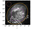 |
Fig. 1 Selected regions and the dark clouds (this work) overlaid on the IHαmap of Sh 2–27. The dashed circle with a radius of 1°.2 is chosen to estimate the off-region used in RMsh2–27estimation (see Sect. 5.3). The dashed box is used for the SF calculations. Each side of the box is ~6°. Contours from the CO emission map of Dame et al. (2001) are overlaid on the H II region to display the structure of the dark clouds. The plus sign represents the location of ζ Oph at (l, b) = (6°.3, +23°.6). The greyscale range is 0–2000 dR. |
3 Data
3.1 Radio polarization
This work is based on the data from S-PASS, a highly sensitive single-dish polarimetric survey of the entire southern sky at 2.3 GHz. The main observational details can be found in Table 1 of Carretti et al. (2019). S-PASS was performed with the Parkes 64 m Radio Telescope Murriyang and S-band (13 cm) receiver. Its angular resolution is 8′.9 and the pixel size is 3′.4. We used the Stokes Q and U maps produced by this survey to estimate polarization angles, which can lead us to calculate B‖-map. The de-biased linear polarized radio intensity of Sh 2–27 is calculated as  (Wardle & Kronberg 1974; Vaillancourt 2006). The associated noise, σQU, was taken from the sensitivity map of S-PASS, assuming that σQ and σU are identical (see Appendix A).
3.2 Ha intensity
As a probe for the electron density, we used the smoothed continuum-subtracted map of Hα surface brightness (IHα) data from SHASSA, which has a noise of ~0.7 Rayleigh (1 R = 106/4π photons cm−2 s−1 sr−1) and an angular resolution of 4′. The map was additionally smoothed to the S-PASS resolution, and resampled onto the S-PASS pixel size using the Python package REPROJECT5. The typical error in IHα after adapting it to S-PASS is 0.6 R.
3.3 Dust reddening
The Galactic dust reddening towards Sh 2–27 was gathered from the Galactic Dust Reddening and Extinction map of Schlegel et al. (1998), and corrected according to the updated estimates by Schlafly & Finkbeiner (2011) (see Sect. 4.2). This map calculates the total dust reddening along the LoS. We used it to correct for the intervening dust extinction along the LoS at the coordinates of Sh 2–27. Similar to the SHASSA map, we smoothed and resampled the map as a final dust extinction map before combining it with other datasets.
4 Method
As the 3D structure of the H II region has an impact on the understanding of its LoS-integrated polarization properties, we modelled the geometrical shape of Sh 2–27 as an ellipsoid to estimate the path length. In the following sections, we introduce our methods of using IHα to estimate ne by calculating emission measure (EM), and using polarization angles to obtain B‖ by estimating RM.
4.1 The ellipsoid model
To estimate the path length through the H II region (the LoS thickness), we modelled Sh 2–27 to be an ellipsoid, which matches its observed shape both in S-PASS and SHASSA.
We applied the general ellipsoid equation rewritten as  in Cartesian coordinates and applied a basic coordinate transformation, where the semi-axes have lengths of a (semi-major radius), b (semi-minor radius), and s (LoS radius or LoS thickness); x and y are in the plane of the sky; and z is along the LoS. Even though the LoS thickness of the H II region is unknown, a reasonable estimate is that s must be between the values of the plane-of-sky axes a and b, hence ne and B‖ are zero for
  We assume a = s here, but we discuss the ramifications of this choice for ne and B‖ in Sect. 7.
At the distance of 180 pc, the corresponding semi-minor axis is 15pc and the semi-major axis is 19 pc. The resulting elliptical region can be seen in Fig. 1. The ellipsoidal shape is geometrically obtained by revolving its surface about its major axis with a central position in (l, b) = (6°.3, +23°.6), and a major axis inclination angle of 45°.8 with respect to the direction of the Galactic longitude. In that way, ζ Oph is in the geometric centre of the H II region. The resulting LoS thickness values can be seen in Fig. 2. As expected from an ellipsoidal shape, the LoS values gradually decrease farther away from the centre.
4.2 Emission measure
The EM is related to ne via the equation
 (2)
(2)
EM can also be derived from the intensity of the Hα line due to recombination transitions of neutral hydrogen atoms, according to (Reynolds et al. 1988):
 (3)
(3)
In the following paragraphs we explain Te, IHα, and eτ.
The electron temperature, Te, is assumed to be ~7000 K for this H ii region6.
The surface brightness values, IHα, from SHASSA are in deci-Rayleigh (dR), and Fig. 3a shows the Hα map of Sh 2–27. Next to the patches of bright Hα emission, the most conspicuous structures are filaments of low Hα emission towards the south of the image. These low-intensity features are caused by the absorption of Hα emission by the dark clouds in front of or partially overlapping with Sh 2–27 (Tachihara et al. 2000; Choi et al. 2015). Figure 1 shows the projected locations of these clouds in CO emission (Dame et al. 2001). As seen in Fig. 3b, the high dust reddening in these clouds is rather pronounced. As the anti-correlation between the Hα emission and the dust extinction indicates, some Hα emission throughout Sh 2–27 is also absorbed by the intervening dust.
We correct for the dust extinction, eτ, by including the optical depth (τ) in the computation of EM in Eq. (3) as follows. To correct for the intervening dust along the LoS, we include an optical depth estimation, τ = 2.44 × E(B – V) (Finkbeiner 2003). The reddening in magnitudes E(B – V) is given in the dust reddening map of Schlegel et al. (1998), corrected by the Schlafly & Finkbeiner (2011) term as E(B – V)S &F = 0.86 × E(B – V)sfd, where S &F symbolizes the Schlafly & Finkbeiner (2011) values derived by Schlegel et al. (1998) values (SFD). Here we assume that the dust is in front of the H ii region and is not mixed in. The maps of E (B – V) and τ are presented in Figs. 3b and 3c, respectively, and as seen, the dust reddening is higher towards the dark clouds, especially towards L204.
Based on the simplifying assumptions on the extinction correction, the absorption by the foreground dark clouds, clearly visible in Fig. 3a, has lessened after dust correction. Likewise, the imprint of the dust map on the EM map has diminished significantly (see Fig. 3d). We assume that the effect of the dust extinction on the EM map is negligible after correction. Moreover, we do not include any background or foreground Hα emission correction as we assume that the EM signal is caused by the H ii region itself due to the lack of the background EM signal surrounding Sh 2–27, as seen in Fig. 3d.
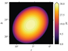 |
Fig. 2 Colour-coded LoS values for each pixel represented by the projected elliptical shape chosen for Sh 2–27. The maximum path length through the H ii region (z-axis) is equal to the major axis of the ellipsoid (38 pc). |
4.3 Electron density
Since the ionized medium of an H ii region is inhomogeneous, the term f stands for a fraction of the volume of dense gas (clumps) to a total volume of an H ii region that is occupied by the clumps. Different approaches to estimate f in H ii regions can be found in earlier studies (e.g. Herter et al. 1982; Kassim et al. 1989; Giammanco et al. 2004). To account for inhomo-geneities of the ISM through the H ii region, we assumed f of the Faraday-rotating gas to be 0.2 (Harvey-Smith et al. 2011), and outside a clump ne is zero. Equation (4) can be used to evaluate the variations in the electron density averaged along the LoS as (Ocker et al. 2020)
 (4)
(4)
We found a median value of  inside the elliptical area to be 7.3 ± 0.1 cm−3, and the resulting map can be seen in Fig. 3e; for the map of
  see Fig. 3f. The high ne values in the extension of L204 at (l, b) ~ (5°, +19°) show the highest dust (Fig. 3b) and the highest uncertainties (Fig. 3f). These values are likely caused by a possible imperfect correction for the dust extinction. Nevertheless, this region falls outside the area where we perform the quantitative analysis of the turbulence (Sect. 6); thus, we do not attempt any further corrections. Figure 4 shows the distribution of ne, as well as the distribution of ne found inside the box in Fig. 1.
5 Analysis of the polarized radio observations
In what follows we briefly introduce the total radio and the polarized radio intensities and describe how we estimate the polarization angles that we used to calculate RMSh2–27 to derive a map of B‖.
5.1 Total radio and polarized radio intensities in Sh 2–27
Figure 5 presents the total radio and polarized radio intensities in Sh 2–27. The total intensity denotes a combination of free-free emission and synchrotron emission, while the polarization only occurs in synchrotron emission. In total intensity the free-free emission may come from where the Stokes I map correlates with the Hα map. In addition, there are three noticeable features in the polarized intensity, which we will discuss in turn: (a) the polarized intensity does not show emission correlating with the total intensity; (b) depolarization canals are visible; (c) there is a highly polarized filament diagonally crossing the H ii region.
Firstly, if there were significant synchrotron radiation emitted by Sh 2–27, there would be accompanying polarized emission. As this is not seen in Fig. 5, synchrotron emission from Sh 2–27 is negligible, supporting the assumption that Sh 2–27 is a Faraday screen, as discussed in Sect. 2.
Secondly, depolarization canals are elongated structures of one beam-width depolarization, without counterparts in total radio intensity (e.g. Haverkorn et al. 2000; Gaensler et al. 2001). They are ubiquitous in radio polarization maps (e.g. Gray et al. 1999; Uyaniker et al. 1999; Haverkorn et al. 2000; Gaensler et al. 2001; Shukurov & Berkhuijsen 2003; Haverkorn & Heitsch 2004; Fletcher & Shukurov 2007). Depolarization canals can be caused by beam depolarization and depth depolarization (Fletcher & Shukurov 2007). Beam depolarization occurs if structures in the Faraday rotating medium give rise to significant gradients in polarization angle within the telescope beam. Depth depolarization occurs when a medium along a LoS is mixed with both a synchrotron-emitting medium and a thermal medium, which causes different polarization angles at different depths in the medium, reducing the observed polarization. We note that this is not the case for Sh 2–27, which does not produce a significant amount of polarized emission itself (see Sect. 2). The observed depolarization canals point towards sharp gradients in Faraday rotation in the H ii region within the S-PASS beam, as might be expected from small-scale structures in the magnetic field and/or electron density.
Lastly, the polarized filament crossing Sh 2–27 is not part of the H ii region, but belongs to a larger configuration of radio-filaments and loops. It can be seen in the WMAP K-band polarization maps of Vidal et al. (2015), where it appears between the filament IX and the Galactic Centre spur (in their Fig. 2), and extends towards the north Galactic pole along with the large-scale magnetic field direction (in their Fig. 1 panel top left). It is not visible either in the lower-frequency radio polarization maps of Thomson et al. (2019) in 300–480 MHz or in the 1.4 GHz all-sky polarization map combined by Reich & Reich (2009). It might be unresolvable because of the low resolution. As there are no depolarization canals across the polarized filament, it has to be in the foreground of the H ii region. The non-zero polarized intensity of the filament contributes to the background intensity, and therefore can still influence the observed polarization angles (Kumazaki et al. 2014), as well as the RM measurements. There may be a hint of the filament in the RM maps (see Fig. 6). However, as these data do not allow quantification or correction of this slight influence, we assume that it is negligible.
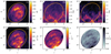 |
Fig. 3 Efficacy of the extinction correction, as described in Sect. 4. (a) IHα; (b) E(B – V); (c) τ; (d) EM (colour-scale saturated to 1000 cm−6 pc, the maximum is 2251 cm−6 pc); (e) ne (colour-scale saturated to 15 cm−3, the maximum is 57.6 cm−3); |

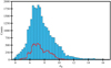 |
Fig. 4 Distribution of ne in the elliptical area selected for Sh 2–27. The overlaid red histogram shows the distribution gathered from the box region shown in Fig. 1. |
5.2 Polarization angle
H ii regions as Faraday screens alter the polarization angle of a traversing electromagnetic wave on the plane of the sky. The polarization angle, χ, can be calculated by using Stokes Q and U:
 (5)
(5)
Following the estimation of the polarization angle, we de-rotated the relevant data in nπ-ambiguity between adjacent data points (i, j) to check if a jump in the angle occurred, caused by a polarization vector that revolved multiple times (n). Hence, we determined the most probable angle relative to a surrounding reference point in the consideration of ∆χ = χ(i+1,j) − χ(i,j) (Brown et al. 2003; Haverkorn et al. 2003; Brentjens & de Bruyn 2005).
The de-rotation is made according to the following equation:
 (6)
(6)
We note that employing this algorithm row by row may result in the nπ-ambiguity being unresolvable in some sequential pixels (only 6 out of 47 073 pixels), which are centred at the following locations (they are left uncorrected): (l, b) = (5°.5, +19°.9), (5°.5, +20°.0), (5°.7, +19°.8), (5°.7, +19°.9), (8°.3, +25°.3), (8°.4, +25°.4). These pixels are in the highest depolarization regions seen in Fig. 5b. The resulting map can be seen in Fig. 6a along with its uncertainty for each data point in Fig. 6b. Additionally, as seen in Fig. 6b, σχ resembles the reverse of Fig. 5b, since σχ ∝ P−1 in Eq. (A.12) of Brentjens & de Bruyn 2005.
To see how the elliptical area that we choose is related to the polarization angle variations, and to the IHα variations, we show a basic model fitting in Fig. 7. This figure shows cuts from the H ii region on both axes of the polarization angle map (Fig. 6a). The ellipsoid parameters that we mention in Sect. 4.1 are fitted to these data. They roughly demonstrate how reasonably the size of the ellipse is determined for the maximum LoS thickness of the H ii region, which is essential for ne and B‖ estimations. Consequently, they can be interpreted as small-scale fluctuations in the magnetic field and/or the electron density, as also indicated by the presence of the depolarization canals.
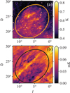 |
Fig. 5 Radio synchrotron emission in the direction of Sh 2–27. Top: total radio intensity (colour-scale saturated to 0.80 K, the maximum is 0.95 K). Bottom: polarized radio intensity. |
5.3 Rotation measure
For a single-frequency polarization measurement of Sh 2–27, we can estimate RMSh2–27 as long as we can treat the H ii region as a Faraday screen (as shown in e.g. Iacobelli et al. 2014; Robitaille et al. 2017, Robitaille et al. 2018, and in Sect. 5.1). Here, we initially assume that the background and foreground RMs are constant (Sun et al. 2007; Xiao et al. 2011; Thomson et al. 2018). This is a reasonable assumption relative to the high RM in the H ii region itself. Each pixel within the elliptic boundary of Sh 2–27 holds that the polarization angle
 (7)
(7)
where λS = 0.13 m is the observing wavelength, RMSh2–27(x, y) is the position-dependent RMSh2–27 of the H ii region itself, RMback is the position-independent background RM, and χ0 is the intrinsic polarization angle assumed to be constant. The polarization angle just off the H ii region is then
 (8)
(8)
hence, RMSh2–27 can be calculated as
 (9)
(9)
where χoff = −1.8 rad. By choosing χoff as the polarization angle value just outside the ellipsoid, which is de-rotated to the value closest to the polarization angle at the edge (as in Sect. 5.2), we avoid the nπ-ambiguity problem here, as χon and χoff individually have an nπ-ambiguity, but χon − χoff does not.
The off-region was chosen as the region close to the edge of Sh 2–27 with the least contaminating emission from other sources. Firstly, on the right side of Fig. 6a there is another H ii region (Sh 2–7) (see Iacobelli et al. 2014). Secondly, an off-region from the bottom left part of Fig. 6a is also not ideal, considering the high errors in the polarization angle (Fig. 6b). However, the off-region as drawn in Fig. 1 seems to be representative because, if we vary the radius or position of the circle in the vicinity, the off-region level does not vary significantly.
The resulting RMSh2–27 map together with its uncertainty can be seen in Figs. 6c and d, respectively. The median RMSh2–27 inside the elliptical area is −126.0 ± 3.1 rad m−2. We estimated  using Eq. (A.2). This approach differs slightly from that of Harvey-Smith et al. (2011), who used RMs of polarized extragalactic point sources from the catalogue of Taylor et al. (2009), and subtracted a small linear gradient in extrinsic RM computed from a region around Sh 2–27. Their
  values are roughly in the range from 75 to 300 rad m−2, and ours in the range of 59 rad
  rad m−2 within the elliptical boundary of the H ii region. These values are generally consistent with each other, although our
  values show a higher maximum than their results. These high values are in regions where Harvey-Smith et al. (2011) do not have coverage of background sources, which makes it impossible to detect these values with their method.
5.4 Magnetic field parallel to the LoS
We derived By for each pixel (i.e. for each LoS) using Eq. (10), which is rewritten from Eq. (1) under the assumption that ne and B‖ are constant along the LoS:
 (10)
(10)
This equation is also strictly valid if ne and B‖ are uncorrelated. Figure 8 displays the result of B‖ along with its uncertainty  using the relation in Eq. (A.5). We estimated B‖ with a median
  of −4.5 ± 0.1 µG inside the elliptical area. We note that the extreme B‖values at the edges of the ellipse are likely caused by overestimation due to the small LoS values.
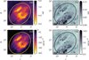 |
Fig. 6 Polarization angle and the rotation measure properties of Sh 2–27. (a)χ; (b) σχ (colour-scale saturated to 0.15 rad, the maximum is 0.70 rad); |

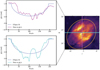 |
Fig. 7 Comparison of the elliptical model to the polarization angle variations in Sh 2–27. Left: nπ-ambiguity corrected polarization angle variations along 1D image slices. Right: colour-coded lines show the data taken from the polarization angle map. A slice of the data in the xy-plane is considered, passing through l = 6° for χ(x) and b = 23° for χ(y), where (l, b) = (6°, 23°) is the centre of the ellipse. |
6 Statistical analysis of turbulence with structure functions
The energy of incompressible and homogeneous turbulence cascades from the largest scales, where energy is deposited to the smallest scales through a dissipation process. If there is no energy input or loss in intermediate scales, this is called Kolmogorov turbulence (Kolmogorov 1941), which represents the turbulence with a basic scaling relation. This scaling is a power law, which can be characterized by a power spectrum (PS) or a structure function (SF). The theory of Kolmogorov (1941) predicts a power spectrum of 3D turbulence with a power-law slope of −11/3. Likewise, SF associated with the predicted 3D Kolmogorov turbulence is scaled by the power-law slope of 5/3 (for a comprehensive summary, see e.g. Thompson et al. 2001, Table 13.2). In 2D, power-law indices of PS and SF are also expected to be consistent with 2D Kolmogorov turbulence with a scaling of −8/3 and 2/3 in the magnetized ISM, respectively (Goldreich & Sridhar 1995; Minter & Spangler 1996; Haverkorn et al. 2004, 2006b; Mao et al. 2010). We note that for other theories of turbulence, the relation between the power-law slopes of PS and SF may be different (e.g. Cho & Lazarian 2009). Structure functions rise as fluctuations increase with larger scales. The scale where a structure function starts to flatten out is the largest scale.
Since PS and SF give the same information (Thompson et al. 2001), to ease comparison with earlier studies we present only SFs here. We also calculated PS of our data, and it gave equivalent results in the slopes. The reliability of SF requires a high-resolution observation as discussed in the study of Lee et al. (2016), which is the case for S-PASS.
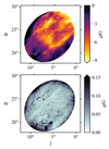 |
Fig. 8 By estimated in Sh 2–27 (top), and its uncertainty (bottom) in the ellipsoid path-length model of Sh 2–27. The colour-scale of B‖ is limited between –9 µG and 0 µG; the minimum is around −18 µG and the maximum is around 3.5 µG. The colour-scale of |

6.1 Structure function
We estimate SFs as follows. The angular separation between two source components is binned with equal lags in logarithmic intervals of a separation by averaging the squares of the differences between the pairs, that is, a radial averaging was made to calculate a 1D SF from the 2D SF. Thereby, a second-order SF is calculated as
 (11)
(11)
where r = (x, y) denotes a 2D position vector on the plane of the sky; δrn is a certain angular separation between the two points; 〈⋯〉r implies an ensemble averaging over all positions with δrn in the relevant interval; and ɡ stands for any function of a field, in our case B‖. We binned these data into bins of 25 pixels. Assuming Gaussian noise, we subtracted the error of the structure function of the noise (SFσ) from  , as done in Haverkorn et al. (2004) and Stil et al. (2011).
One issue to take into consideration in the calculation of  is that the pixel sizes in longitude and latitude are not equal due to the projection, which might be offset by including a factor cos(latitude) to the longitude coordinate. As Sh 2–27 is centred at a latitude of ~23°, the distortion is not as extreme, but it is expanded by ~9% with respect to the latitude. A correction for this effect is included in our estimations, although it did not make any significant change in the
  slopes.
The  is determined within the box region in Fig. 1. The resulting
  can be seen in Fig. 9. We note that the error bars of
  are smaller than the plot symbols. Because small-scale structures are smoothed out below the beam-size,
  is reliable down to the S-PASS resolution (8′.9). Additionally, in a box inside the H ii region’s projected area,
  is reliable up to about half the box, that is, below ~180′. Consequently, any fluctuations on scales larger than this are unreliable.
The  shows a power-law behaviour with a power-law slope of 1.4 that fits the data between 10′ and 50′. On scales larger than that the power-law slope decreases to a flat
  on a scale of ~10 pc, which corresponds roughly to half of the box. On the largest scales,
  seems to turn up again, which is an artefact due to the poor sampling of very large scales in the box. It is tempting to interpret the turnover scale of ~ 10 pc as the outer scale of the turbulence. However, since this scale is comparable to the size of the box, we cannot be sure whether the turnover is due to the finite box size. The power-law slope of 1.4 is indeed higher than the Kolmogorov slope. Hence, to test the dependency of the slope of the estimated turbulent B‖on the actual magnetic field
  , and to investigate whether the turnover scale is due to the outer scale of the turbulence or due to the box size, we designed simulations of an ellipsoidal H ii region containing an input ne and an input turbulent magnetic field. We describe the details of these simulations in the next section.
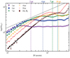 |
Fig. 9 Structure functions of the observed (black) and the simulated B‖ with different outer scales. The outer scales (top) are related to each SF, coded in the same colour. The teal line represents half of the box size. The black line shows the power-law slope of 1.4. The grey line shows the 2/3 Kolmogorov scaling. |
6.2 Synthetic models
Synthetic models with Kolmogorov scaling can give us an idea of the observed turbulence in the presence of Sh 2–27. In that sense, introducing different outer scales to the synthetic models is useful to test the scale where the observed  flattens.
We calculated the  of the simulated fields within the same elliptical area as the observations by focusing on the data inside the same box region shown in Fig. 1. More specifically, the simulations were conducted in a cubic domain that encloses the ellipsoid with a numerical resolution of 2563 (δx ≃ 0.2 pc), which gives the grid the same size as that of the observation: (major axis in pc)/(major axis in pixels) = 19/104 ~ 0.18 pc. We note that we show the angular values in the final results.
Initially, we built the synthetic models with a turbulent magnetic field represented by a 3D PS according to two power laws as
 (12)
(12)
where the wave number of the turnover kinner is associated with the outer scale Louter as Louter ≡ 2π/kinner. We note that a LoS averaging for ne and B‖can also mimic a 3D spectrum (Sridhar & Goldreich 1994); in other words, for 3D Kolmogorov turbulence the power-law scaling slope is −11/3 as PS3D(k)dk ∝ k−11/3. The full 3D magnetic field may indeed have a Kolmogorov spectrum, but we only probe B‖ here. However, according to Chepurnov (1998), if the original magnetic field has a 3D Kolmogorov signature, the parallel component may be expected to show a 3D Kolmogorov-like spectrum as well. Integrating this quantity over the LoS would then result in a 2D Kolmogorov spectrum in PS with a power-law slope of −8/3, and a 2D SF power-law slope of 2/3.
Another significant aspect of turbulent B‖ in this study to be noted is that it is derived from the RMSh2–27 map (Fig. 6c), and it is a LoS integration of 3D By weighted by ne and path length. Therefore, Eq. (10) only holds if ne and B‖are not correlated along any LoS. In the case of a correlation (either positive or negative), this equation will generate overestimated or underestimated B‖ (see Beck et al. 2003). Consequently, if the SF of ne has a Kolmogorov scaling, we can assume that Kolmogorov turbulence in B‖ will result in Kolmogorov turbulence in the SF of RM.
The initial ne is set to be constant (7.3 cm−3) across the H ii region (ne = 0 outside the ellipse). We note that we also tested a turbulent ne under the same conditions; however, since it gave the same  slopes, we continue our analysis with the constant ne.
The simulated turbulent B‖ follows a power law with random phases, according to Eq. (12). The root mean square of B‖ is set to be 6.0 µG. The value of Louter is set to be between 2 pc and 10 pc with a step size of 1 pc. We also computed a separate Louter (20 pc) to test the effect of a larger scale than the computational domain on the flattening. Therefore, the Fourier components of B‖ are drawn from a 3D Gaussian random field in Fourier space with different outer scales. The simulated B‖ follows a PS, where α is fixed as 2 (for k ≤ kinner) and −9/3 ≤ β ≤ −5/3, where β = −5/3 corresponds to the Kolmogorov slope (for k > kinner). By following the same procedure as for the observations, we determined EM and RM, and subsequently used Eq. (10) to calculate the synthetic B‖.
After setting up all the parameters mentioned above, we ran different tests to determine the outer scale, and to test the reliability of the simulations. Their key steps are as follows: (i) testing the effect of various outer scales on the flattening of  on large scales; (ii) taking into consideration the flattening of
  on small scales; (iii) addressing the effect of the different realizations of the turbulence; (iv) testing the effect of the different input slopes on the flattening. The results are the described below.
In step (i), we computed the simulated  with different outer scales to test the starting point of the flattening under different scenarios. In addition to the observed
  , Fig. 9 shows the simulated
  computed with different outer scales up to 20 pc, an input B‖ (–4.5 µG), and the Kolmogorov slope (β = −5/3). The amplitudes of the simulated SFs were set arbitrarily such that the observed
  and simulated
  are distinguishable in the presentation.
In step (ii), the turnovers on scales smaller than 10 pc in the  slopes (Fig. 9) start flattening on scales smaller than the input outer scales. In addition, turnovers at 10 pc and 20 pc are not distinguishable since the computational domain is limited to the size of the box.
In step (iii), we test whether the different behaviours of the flattening on the large angular scales in Fig. 9 is due to different realizations of the turbulence. We made ten representative realizations using 10 pc as the outer scale, and with an input magnetic field (−4.5 µG) and Kolmogorov slope (β = −5/3) as seen in Fig. 10. The results show that the slopes are consistent with each other on the small scales, but above the angular scale of ~50′ the structure functions start to flatten in some realizations. Moreover, the structures on large scales (>50′) are different from each other, confirming our earlier point that they are due to inadequate sampling of the largest scales.
In step (iv), as seen in Fig. 9, the power-law indices of the observed and simulated  are slightly steeper than the Kolmogorov slope (2/3), up to a scale of ~50′. A 1D PS Kolmogorov slope of −5/3 in the input magnetic field spectrum, therefore, results in a steeper output slope of
  . Figure 11 shows the simulations with various input magnetic field slopes (− 9/ 3 ≤ β ≤ − 5/3), which points out that the output slopes of the simulated SFs slightly increase with the increasing input magnetic field slopes.
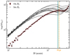 |
Fig. 10 Structure functions of the observed and simulated B‖. Each simulated |

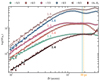 |
Fig. 11 Structure functions of the observed (black) and simulated B‖. Each simulated |


7 Discussion
In this section we interpret the results of the measured magnetic field fluctuations. In Sect. 7.1, we discuss the apparent fluctuations in the magnetic field. In Sect. 7.2, the SFs of the magnetic field are discussed.
7.1 ne and B‖
Several parameters affect the estimation of ne and B‖. We made an assumption of the LoS path length through Sh 2–27, and the filling factor is very uncertain. The initial assumption on the LoS path length is that it is equal to the major axis of the ellipse instead of the minor axis. Then,  and
and  are estimated as 8.2 ± 0.1 cm−3 and −4.8 ± 0.1 µG, respectively. This means that selecting a different path length can affect the results as
  µG. Similarly, to see the changes when adopting different f values, variations in both ne and B‖ can be taken into account in proportion to f−1/2 (see Eqs. (4) and (10)), given that f may not be uniform across the region.
As seen in Fig. 8 in the blob-shaped extension of L204, B‖ values are the lowest and  values are the highest when E(B − V) is mostly high (see Fig. 3b). This relationship may be explained by the high values of τ leading to high
  . Additionally, it can be clearly seen that
  in the low polarized intensity regions (Fig. 6b) is higher than in polarized regions. Hence, by evaluating Eq. (A.6), the analogy between
  and the depolarization canals can be shown, which points out that weak polarization signals cause the high uncertainties of B‖ (see Fig. 8b).
In Fig. 8, multiscale structures in B‖ are visible, possibly indicative of a turbulent magnetic field. Another filament-shaped structure is noticeably oriented from north-west to south-east, which is roughly parallel to the foreground polarized filament that is mentioned in Sect. 5. We only see this filament in the B‖-map. Even though it is not visible in the EM or RMSh2–27 maps, it has to be present in one or both of these, as B‖ is created by these maps. As its orientation is similar to the orientation of the foreground polarized filament mentioned in Sect. 5.1, it is likely that this filament is aligned with some type of large-scale magnetic field (see Vidal et al. 2015) in and around the H ii region. The filament might be connected to the H ii region or might be located in the foreground. If the latter were the case, the filament would be located in a lower-density environment, which would indicate an unrealistically high magnetic field strength to attain the observed RM (Eq. (10)). Therefore, we conclude that the filament of enhanced magnetic field strength is associated with the H ii region, and pointed in a direction of a large-scale magnetic field piercing the H ii region.
Comparison to previous studies
Our result of  broadly supports the previous research in Sh 2–27. Reynolds & Ogden (1982) estimated ne in Sh 2–27 as ~3.8 cm−3 using the lines of Hα and [N ii] λ6584, which is higher than our average electron density along the LoS, ~1.5 cm−3 (〈n〉 = f ne). Moreover, Wood et al. (2005) found ne ~ 2 cm−3 for Sh 2–27, and our result of 〈n〉 is compatible with their result. Additionally, 7.3 ± 0.1 cm−3 is consistent with the value derived by Harvey-Smith et al. (2011) within 1σ (ne = 10.6 ± 2.8 cm−3). The slight difference is likely to be related to the estimated path length that depends on the assumed geometry of the H ii region, the volume filling factor, and the method used to account for the contribution of the dust reddening. They assumed that Sh 2–27 is spherical and that the volume filling factor is 0.1, and they employed a mean dust reddening value (0.47) from Schlegel et al. (1998).
Our resulting  lies well within the ranges of previous studies (see Table 1) that used Faraday rotation of the polarized radio synchrotron emission observations in some H ii regions. Using Faraday rotation of the extragalactic background sources, Heiles & Chu (1980) and Heiles et al. (1981) estimated
  from 1 to 20 µG in the Galactic H ii regions S117, S119, S232, and S264. Mitra et al. (2003) found
  of Sh 2–205 as ~5.7 µG, using RM and dispersion measure of the pulsars PSR J2337+6151 and PSR J0357+5236. The study of the W3/W4/W5/HB3 complex by Gray et al. (1999) specified an average upper limit for the H ii region W4 as ~20 µG. Sun et al. (2007) found
  ~3.9 µG and ~6.4 µG for the H ii regions G124.9+0.1 and G125.6–1.8, respectively. Harvey-Smith et al. (2011) used RMs from the Taylor et al. (2009) catalogue, and obtained
  from 2 to 6 µG in the five Galactic H ii regions (Sh 2–27, Sh 2–264, Sivan 3, Sh 2–171, and Sh 2–220). However, H ii regions of unusually high ne (~350 cm−3) may have higher magnetic field, for example By ~36 µG, as observed in NGC 6334A (Rodrígez et al. 2012). Another point worth noting is that the Taylor et al. (2009) catalogue is missing some sources of high RMs in this region, which may cause biased results, and the real RM for Sh 2–27 that is calculated from the extragalactic sources might be higher than these results (see Stil & Taylor 2007).
The value of  found in Sh 2–27 is in agreement with the diffuse ISM magnetic field (see Crutcher 2007), which may be detected by the high ne in the H ii region, as also previously pointed out by Harvey-Smith et al. (2011).
Values of  estimated in other H ii regions by using Faraday rotation of the polarized radio synchrotron emission observations.
7.2 Structure functions
In this section we discuss the outer scales of fluctuations obtained and compare them to synthetic models (Sect. 7.2.1), and we compare these results to previous studies (Sect. 7.2.2).
7.2.1 Outer scales and turbulent power-law slope
In the observed  the flattening occurs almost at the maximum scale of the data (~180′), which corresponds to a scale of ~10 pc (assuming a distance to the H ii region of 180 pc). The question of whether this turnover scale corresponds to the outer scale of turbulence can be answered with the help of the results of the numerical simulations in Sect. 6.2. The turbulent (input) outer scales smaller than 10 pc can be seen to have smaller (output) turnover scales. In addition, no clear distinction can be made between the turnover scales for the turbulent outer scales of 10 pc and higher; see result ii) in Sect. 6.2. This means that we can only give a lower limit of ~10 pc to the observed maximum scale of fluctuations. If the turbulence inside the H ii region is a continuation of general interstellar turbulence in the ionized environment around a massive star, the outer scale of the fluctuations may be even larger than the H II region itself.
Result iii) in Sect. 6.2 shows that at scales larger than ~50′, the effect of different realizations of the turbulence becomes noticeable, indicating that to determine the  slopes, we should not take scales >50′ into account.
Result iv) shows that an input 3D Kolmogorov slope (−11/3) of the magnetic field in the simulations gives an output slope of 1.4, which is slightly steeper than the 2D Kolmogorov value (>2/3). Figure 11 shows that for steeper input magnetic field spectra the output  slopes also return slightly steeper values. As we stated in Sect. 6.2, the input of the constant ne and turbulent ne in the simulations did not change the resulting
  slope, thus the density weighting of Eq. (10) is not likely to be responsible for not retrieving the 2/3 slope. Therefore, the reason is likely to be related to the shape of the object including an additional source of structure from the varying path length through the object, which would increase at larger scales. Nevertheless, the
  slope calculated from the observations is consistent with the
  slope of the simulations for a Kolmogorov-like input spectrum of the magnetic field. Therefore, we conclude that our observations are consistent with a turbulent magnetic field with a Kolmogorov slope inside Sh 2–27.
We note that even if the SF slopes are consistent with the Kolmogorov turbulence, complexities still remain in translating these slopes to physical quantities such as the magnetic field. In our calculations, the following approximations induce uncertainties: (a) that the integration over the path length is approximated by f s; (b) that a uniform Te and f across the region are adopted; (c) that spatial irregularities in the observed quantities of EM and RMSh2–27, and in the LoS dependency of B‖ (B‖ ∝ s−1/2) may occur.
These results suggest that SFs of observed B‖ -maps that are computed via polarization observations can be used to characterize turbulence inside H II regions. However, this method must be approached with some caution as the size of the computational domain, adopted geometry, and stochasticity may play a significant role in the interpretation of slopes and outer scales.
7.2.2 Comparison to previous studies
As mentioned in Sect. 6.2, we find a Kolmogorov-slope, and a lower limit to the outer scale of about 10 pc in Sh 2–27. If the observed turbulent magnetic field in Sh 2–27 is affiliated with the turbulence in the general warm ionized ISM, as argued before, it is useful to compare it to earlier studies of turbulence in this medium, considering turbulent slopes and outer scales. Stil et al. (2011) mapped out SFRM across the northern sky and found a slope of ~1.3 towards Sh 2–27, which is very close to our scaling.
The analysis of turbulent velocity structure in ionized gas is likely connected to its gas density and magnetic field fluctuations. Power spectra of velocity fluctuations in H II regions can show Kolmogorov-like spectra (Roy & Joncas 1985; Miville-Deschenes et al. 1995), although not necessarily (O'Dell & Castaneda 1987; Medina-Tanco et al. 1997; Chakraborty & Anandarao 1999; Lagrois & Joncas 2009; Melnick et al. 2021).
Previous works (e.g. Medina-Tanco et al. 1997) have also attempted to find an outer scale in an H II region by focusing on large scales. They found an outer scale of 10 pc in the extra-galactic H II region NGC 604, which was attributed to a possible stellar formation event.
In the literature, Kolmogorov-like turbulence was found in the ISM in electron density fluctuations (e.g. Armstrong et al. 1981; Higdon 1984; Armstrong et al. 1990; Wang et al. 2005; Chepurnov & Lazarian 2010). Spangler & Gwinn (1990) inspected the interstellar electron density PS in radio scattering measurements, and found consistency with the predicted Kolmogorov slope of −11/3. Minter & Spangler (1996) examined EM and RM fluctuations transitioned from 3D Kolmogorov-like turbulence to 2D Kolmorogov-like turbulence at large scales, and conjectured that this was due to a stratified environment of a massive star.
Even though the measured SF slopes here are compatible with Kolmogorov-like turbulence, the turbulence in H II regions is compressible (Miville-Deschenes et al. 1995), which indicates that in reality the turbulence is more complex than the Kolmogorov theory.
Thus far, the previous studies on H II regions (e.g. Miville-Deschenes et al. 1995; Arthur et al. 2016) typically studied turbulent fluctuations on much smaller scales than the scales probed here. If the outer scale of the fluctuations represents the outer scale of the turbulence, it would be comparable to the size of the H II region or even exceed it. In the latter case, the turbulence we detect inside the H II region may well be a probe of the turbulence in the general ISM, which happens to be highlighted by the high electron density in the H II region (Spangler 2021).
8 Conclusions
In this study, we used the Faraday rotation of the polarized radio synchrotron emission data from S-PASS at 2.3 GHz and the Hα data from SHASSA to determine B‖ in Sh 2–27 for each LoS. This lead to a search for the imprint of the turbulence and its outer scale on the B‖-map of the H II region by using the second-order SF. The following conclusions can be drawn from this study:
(i) By making use of three observations (linear radio polarization, Hα, and dust) we computed the maps of ne and B‖ of Sh 2–27. We estimated  and
and  in Sh 2–27 as 7.3 ± 0.1 cm−3 and -4.5 ± 0.2 µG, respectively. The B‖-map for each LoS shows multiscale structures and variations (−18 µG < B‖ < 3.5 µG) across the chosen elliptical area of the H II region.
(ii) The power-law slopes of SFs are compatible with a Kolmogorov-like spectrum of the 3D magnetic field inside the H ii region, as simulations reveal.
(iii) The observed and simulated SFs imply that the outer scale of the turbulent fluctuations is larger than 10 pc, which is comparable to the size of the H II region. This may indicate that the turbulence probed here is the interstellar turbulence in the general ISM, cascading from the larger scales than the size of the H II region in the ambient medium, which is highlighted by Sh 2–27.
By virtue of well-resolved observations, this study presents a detailed map of By for each LoS along with a study of the turbulent magnetic field properties in the H II region Sh 2–27. Further research in other H II regions would be an indispensable next step in understanding the turbulence of the magnetic field in these objects, and the ISM.
Acknowledgements
We thank the referee for a constructive report. NCR thanks Alec J.M. Thomson for help in constructing the power spectra, Luke Pratley and Anna Ordog for discussions, and Karel D. Temmink for suggestions. This work is part of the joint NWO-CAS research programme in the field of radio astronomy with project number 629.001.022, which is (partly) financed by the Dutch Research Council (NWO). MH acknowledges funding from the European Research Council (ERC) under the European Union’s Horizon 2020 research and innovation programme (grant agreement no. 772663). JMS acknowledges the support of the Natural Sciences and Engineering Research Council of Canada (NSERC), 2019-04848. The Dunlap Institute is funded through an endowment established by the David Dunlap family and the University of Toronto. BMG acknowledges the support of the Natural Sciences and Engineering Research Council of Canada (NSERC) through grant RGPIN-2015-05948, and of the Canada Research Chairs program. XS is supported by the National Natural Science Foundation of China (Grant No. 11763008). JH is supported by the National Natural Science Foundation of China: 11988101. XS, JH and XG are funded by the CAS-NWO cooperation programme (Grant No. GJHZ1865). This work has made use of S-band polarization All-Sky Survey (S-PASS) data. We acknowledge the Southern H-Alpha Sky Survey Atlas (SHASSA), which is supported by the National Science Foundation (Gaustad et al. 2001). This work made use of Astropy (http://www.astropy.org) a community-developed core Python package for Astronomy (Astropy Collaboration 2018), NumPy (https: //numpy.org/) (Oliphant 2006; van der Walt et al. 2011), and Matplotlib (http://www.matplotlib.org/) python module (Hunter 2007). We have made use of the “inferno” and “bone” colour-maps, and colour-blind-friendly figures.
Appendix A Propagation of errors in estimations
We included the errors for each data point in our estimations by adapting the propagation of error calculations (Squires 2001; Brentjens & de Bruyn 2005; Hughes & Hase 2010).
We derive the uncertainty of polarization angles following Brentjens & de Bruyn (2005) as
 (A.1)
(A.1)
where σQ = σU = σQU, which leads to  by
by
 (A.2)
(A.2)
The uncertainty of EM is estimated as
 (A.3)
(A.3)
where  = 0.6 R for each data point (after convolution to S-PASS), and στ can be derived from the dust map by using the Python STATISTICS module. Within the same adaption the uncertainty of ne is
 (A.4)
(A.4)
Finally, the uncertainty of B‖ is
 (A.5)
(A.5)
which can also be rewritten as
 (A.6)
(A.6)
so that if we consider  from Eq. (A.12) in Brentjens & de Bruyn 2005, the relationship between the uncertainties of the magnetic field and the depolarization canals, in our study, can be found from
  , where
 (A.7)
(A.7)
References
- Armstrong, J. W., Cordes, J. M., & Rickett, B. J. 1981, Nature, 291, 561 [NASA ADS] [CrossRef] [Google Scholar]
- Armstrong, J. W., Coles, W. A., Kojima, M., & Rickett, B. J. 1990, ApJ, 358, 685 [NASA ADS] [CrossRef] [Google Scholar]
- Arthur, S. J., Medina, S. N. X., & Henney, W. J. 2016, MNRAS, 463, 2864 [Google Scholar]
- Astropy Collaboration (Price-Whelan, A.M., et al.) 2018, AJ, 156, 123 [NASA ADS] [CrossRef] [Google Scholar]
- Beck, R., Shukurov, A., Sokoloff, D., & Wielebinski, R. 2003, A&A, 411, 99 [NASA ADS] [CrossRef] [EDP Sciences] [Google Scholar]
- Blaauw, A. 1961, Bull. Astron. Inst. Netherlands, 15, 265 [NASA ADS] [Google Scholar]
- Brandenburg, A., & Subramanian, K. 2005, Phys. Rep., 417, 1 [NASA ADS] [CrossRef] [Google Scholar]
- Brentjens, M. A., & de Bruyn, A. G. 2005, A&A, 441, 1217 [NASA ADS] [CrossRef] [EDP Sciences] [Google Scholar]
- Brown, J. C., Taylor, A. R., & Jackel, B. J. 2003, ApJS, 145, 213 [NASA ADS] [CrossRef] [Google Scholar]
- Burn, B. J. 1966, MNRAS, 133, 67 [Google Scholar]
- Carretti, E., Haverkorn, M., Staveley-Smith, L., et al. 2019, MNRAS, 489, 2330 [Google Scholar]
- Chakraborty, A., & Anandarao, B. G. 1999, A&A, 346, 947 [NASA ADS] [Google Scholar]
- Chepurnov, A. V. 1998, Astron. Astrophys. Trans., 17, 281 [Google Scholar]
- Chepurnov, A., & Lazarian, A. 2010, ApJ, 710, 853 [NASA ADS] [CrossRef] [Google Scholar]
- Chevalier, R., & Fransson, C. 1984, ApJ, 279, L43 [NASA ADS] [CrossRef] [Google Scholar]
- Cho, J., & Lazarian, A. 2009, ApJ, 701, 236 [NASA ADS] [CrossRef] [Google Scholar]
- Choi, Y. J., Min, K. W., & Seon K.I. 2015, ApJ, 800, 132 [NASA ADS] [CrossRef] [Google Scholar]
- Costa, A. H., Spangler, S. R., Sink, J. R., Brown, S., Mao, S. A. 2016, ApJ, 821, 92 [NASA ADS] [CrossRef] [Google Scholar]
- Crutcher, R. M. 2007, in IAU Symp. 242, Magnetic Fields in the Non-Masing ISM, eds. J.M. Chapman, & W.A. Baan (Cambridge: Cambridge University Press), 47 [Google Scholar]
- Dame, T. M., Hartmann, D., & Thaddeus, P. 2001, ApJ, 547, 792 [Google Scholar]
- De Young, D. S. 1980, Astrophys. J. 241, 89 [Google Scholar]
- Draine, B. T., & Kreisch, C. D. 2018, ApJ, 862, 30 [NASA ADS] [CrossRef] [Google Scholar]
- Elmegreen, B. G., & Scalo, J. 2004, ARA&A, 42, 211 [Google Scholar]
- Ferrière, K. M. 2001, RvMP, 73, 1031 [Google Scholar]
- Finkbeiner, D. P. 2003, ApJS, 146, 407 [Google Scholar]
- Fletcher, A., & Shukurov, A. 2007, EAS Publ. Ser., 23, 109 [NASA ADS] [CrossRef] [EDP Sciences] [Google Scholar]
- Gaensler, B. M., Dickey, J. M., McClure-Griffiths, N. M., et al. 2001, ApJ, 549, 959 [Google Scholar]
- Gaia Collaboration (Prusti, T., et al.) 2016, A&A, 595, A1 [NASA ADS] [CrossRef] [EDP Sciences] [Google Scholar]
- Gaia Collaboration (Brown, A.G.A., et al.) 2018, A&A, 616, A1 [NASA ADS] [CrossRef] [EDP Sciences] [Google Scholar]
- Gao, X. Y., Reich, W., Han, J. L., et al. 2010, A&A, 515, A64 [NASA ADS] [CrossRef] [EDP Sciences] [Google Scholar]
- Gaustad, J. E., McCullough, P. R., Rosing, W., van Buren, D. 2001, PASP, 113, 1326 [NASA ADS] [CrossRef] [Google Scholar]
- Giacalone, J. 2017, ApJ, 848, 123 [NASA ADS] [CrossRef] [Google Scholar]
- Giammanco, C., Beckman, J. E., Zurita, A., & Relano, M. 2004, A&A, 424, 877 [NASA ADS] [CrossRef] [EDP Sciences] [Google Scholar]
- Goldreich, P., & Sridhar, S. 1995, ApJ, 438, 763 [Google Scholar]
- Gray, A. D., Landecker, T. L., Dewdney, P. E., et al. 1999, ApJ, 514, 221 [NASA ADS] [CrossRef] [Google Scholar]
- Harvey-Smith, L., Madsen, G. J., & Gaensler, B. M. 2011, ApJ, 736, 83 [CrossRef] [Google Scholar]
- Haverkorn, M., & Heitsch, F. 2004, A&A, 421, 1011 [NASA ADS] [CrossRef] [EDP Sciences] [Google Scholar]
- Haverkorn, M., Katgert, P., & de Bruyn, A. G. 2000, A&A, 356, L1 [Google Scholar]
- Haverkorn, M., Katgert, P., & de Bruyn, A. G. 2003, A&A, 403, 1031 [NASA ADS] [CrossRef] [EDP Sciences] [Google Scholar]
- Haverkorn, M., Gaensler, B. M., McClure-Griffiths, N. M., Dickey, J. M., & Green, A. J. 2004, ApJ, 609, 776 [NASA ADS] [CrossRef] [Google Scholar]
- Haverkorn, M., Gaensler, B. M., Brown, J. A. C., et al. 2006, Astron. Nachr., 327, 483 [NASA ADS] [CrossRef] [Google Scholar]
- Heiles, C., & Chu, Y.-H. 1980, ApJ, 235, L105 [NASA ADS] [CrossRef] [Google Scholar]
- Heiles, C., Chu, Y. H., & Troland, T. H. 1981, ApJ, 247, L77 [NASA ADS] [CrossRef] [Google Scholar]
- Herter, T., Briotta, D. A.Jr., Gull, G.E., Shure, M.A., & Houck, J.R. 1982, ApJ, 262, 164 [NASA ADS] [CrossRef] [Google Scholar]
- Higdon, J. C. 1984, ApJ, 285, 109 [Google Scholar]
- Hughes, I., & Hase, T. P. A. 2010. Measurements and Their Uncertainties: A Practical Guide to Modern Error Analysis (New York: Oxford University Press) [Google Scholar]
- Hunter, J. D. 2007, Comput. Sci. Eng., 9, 90 [NASA ADS] [CrossRef] [Google Scholar]
- Iacobelli, M., et al. 2014, A&A, 566, A5 [NASA ADS] [CrossRef] [EDP Sciences] [Google Scholar]
- Kassim, N. E., Weiler, K. W., Erickson, W. C., & Wilson, T. L. 1989, ApJ, 338, 152 [NASA ADS] [CrossRef] [Google Scholar]
- King, P. K., Chen, C.-Y., Fissel, L. M., & Li, Z.-Y. 2019, MNRAS, 490, 2 [Google Scholar]
- Kolmogorov, A. 1941, Akad. Nauk SSSR Dokl., 30, 301 [Google Scholar]
- Kumazaki, K., Akahori, T., Ideguchi, S., Kurayama, T., & Takahashi, K. 2014, PASJ, 66, 61 [NASA ADS] [Google Scholar]
- Lagrois, D., & Joncas, G. 2009, ApJ, 700, 1847 [NASA ADS] [CrossRef] [Google Scholar]
- Lazarian, A. 2009, SSRv, 143, 357 [NASA ADS] [Google Scholar]
- Lazarian, A., & Cho, J. 2004, Ap&SS, 292, 29 [NASA ADS] [CrossRef] [Google Scholar]
- Lee, H., Lazarian, A., & Cho, J. 2016, ApJ, 831, 77 [NASA ADS] [CrossRef] [Google Scholar]
- Li, H.-B., Dowell, C. D., Goodman, A., Hildebrand, R., & Novak, G. 2009, ApJ, 704, 891 [NASA ADS] [CrossRef] [Google Scholar]
- Lynds, B. T. 1962, ApJS, 7, 1 [NASA ADS] [CrossRef] [Google Scholar]
- Madsen, G. J., Reynolds, R. J., & Haffner, L. M. 2006, ApJ, 652, 401 [CrossRef] [Google Scholar]
- Mao, S. A., Gaensler, B. M., Haverkorn, M., et al. 2010, ApJ, 714, 1170 [NASA ADS] [CrossRef] [Google Scholar]
- Martin-Alvarez, S., Devriendt, J., Slyz, A., & Teyssier, R. 2018, MNRAS, 479, 3343 [NASA ADS] [CrossRef] [Google Scholar]
- McKee, C. F., & Ostriker, E. C. 2007, ARA&A, 45, 565 [Google Scholar]
- Medina-Tanco, G. A., Sabalisck, N., Jatenco-Pereira, V., & Opher, R. 1997, ApJ, 487, 163 [Google Scholar]
- Melnick, J., Terlevich, R., Tenorio-Tagle, G., Telles, E., & Terlevich, E. 2021, A&A, 649, A175 [NASA ADS] [CrossRef] [EDP Sciences] [Google Scholar]
- Mestel, L., & Spitzer, L.Jr., 1956, MNRAS, 116, 503 [NASA ADS] [CrossRef] [Google Scholar]
- Minter, A. H., & Balser, D. 1997, ApJ, 484, L133 [NASA ADS] [CrossRef] [Google Scholar]
- Minter, A. H., & Spangler, S. R. 1996, ApJ, 458, 194 [NASA ADS] [CrossRef] [Google Scholar]
- Mitra, D., Wielebinski, R., Kramer, M., & Jessner, A. 2003, A&A, 398, 993 [NASA ADS] [CrossRef] [EDP Sciences] [Google Scholar]
- Miville-Deschenes, M.-A., Joncas, G., & Durand, D. 1995, ApJ, 454, 316 [NASA ADS] [CrossRef] [Google Scholar]
- Nicholls, D. C., Dopita, M. A., & Sutherland, R. S. 2012, ApJ, 752, 148 [NASA ADS] [CrossRef] [Google Scholar]
- O’Dell, C., & Castaneda, H.O. 1987, ApJ, 304, 767 [Google Scholar]
- Ocker, S. K., Cordes, J. M., Chatterjee, S. 2020, ApJ, 897, 124 [NASA ADS] [CrossRef] [Google Scholar]
- Oliphant, T. E. 2006. A Guide to NumPy (USA: Trelgol Publishing) [Google Scholar]
- Ostriker, E. C., Stone, J. M., & Gammie C.F. 2001, ApJ, 546, 980 [NASA ADS] [CrossRef] [Google Scholar]
- Pan, L., & Padoan, P. 2009, ApJ, 692, 594 [NASA ADS] [CrossRef] [Google Scholar]
- Reich, W., & Reich, P. 2009, IAU Symp., 259, 603 [NASA ADS] [Google Scholar]
- Reynolds, R. J. 1988, ApJ, 333, 341 [NASA ADS] [CrossRef] [Google Scholar]
- Reynolds, R. J., & Ogden P.M. 1982, AJ, 87, 2 [Google Scholar]
- Robitaille, J. F., Scaife, A. M. M., Carretti, E., et al. 2017, MNRAS, 468, 2957 [NASA ADS] [CrossRef] [Google Scholar]
- Robitaille, J. F., Scaife, A. M. M., Carretti, E., et al. 2018, A&A, 617, A101 [NASA ADS] [CrossRef] [EDP Sciences] [Google Scholar]
- Rodriguez, L. F., Gomez, Y., & Tafoya, D. 2012, MNRAS, 420, 279 [NASA ADS] [CrossRef] [Google Scholar]
- Roy, J.-R., & Joncas, G. 1985, ApJ, 288, 142 [NASA ADS] [CrossRef] [Google Scholar]
- Scalo, J. M. 1984, ApJ, 277, 556 [NASA ADS] [CrossRef] [Google Scholar]
- Schlafly, E. F., & Finkbeiner, D. P. 2011, ApJ, 737, 103 [Google Scholar]
- Schlegel, D. J., Finkbeiner, D. P., & Davis, M. 1998, ApJ, 500, 525 [Google Scholar]
- Sharpless, S. 1959, ApJS, 4, 257 [Google Scholar]
- Shukurov, A., & Berkhuijsen, E. M. 2003, MNRAS, 342, 496 [NASA ADS] [CrossRef] [Google Scholar]
- Spangler, S. R. 2007, ASPC, 265, 307 [NASA ADS] [Google Scholar]
- Spangler, S. R., 2021, Res. Notes AAS, 5, 12 [NASA ADS] [CrossRef] [Google Scholar]
- Spangler, S. R., & Gwinn, C. R. 1990, ApJ, 353, L29 [NASA ADS] [CrossRef] [Google Scholar]
- Squires, G. L. 2001, Practical Physics (Cambridge University Press) [CrossRef] [Google Scholar]
- Sridhar, S., & Goldreich, P. 1994, ApJ, 432, 612 [Google Scholar]
- Stil, J.M., & Taylor, A.R. 2007, ApJL, 663, 21 [Google Scholar]
- Stil, J. M., Taylor, A. R., & Sunstrum, C. 2011, ApJ, 726, 4 [NASA ADS] [CrossRef] [Google Scholar]
- Sivan, J. P. 1974, A&AS, 16, 163 [NASA ADS] [Google Scholar]
- Sun, X. H., Han, J. L., Reich, W., et al. 2007, A&A, 463, 993 [NASA ADS] [CrossRef] [EDP Sciences] [Google Scholar]
- Tachihara, K., Abe, R., Onishi, T., Mizuno, A., & Fukui, Y. 2000, PASJ, 52, 1147 [NASA ADS] [CrossRef] [Google Scholar]
- Tachihara, K., Saigo, K., Higuchi, A.E., et al. 2012, ApJ, 754, 95 [NASA ADS] [CrossRef] [Google Scholar]
- Taylor, A. R., Stil, J. M., & Sunstrum, C. 2009, ApJ, 702, 1230 [Google Scholar]
- Thomson, A. J. M., McClure-Griffiths, N. M., Federrath, C., et al. 2018, MNRAS, 479, 5620 [Google Scholar]
- Thomson, A. J. M., Landecker, T.L., Dickey, J.M., et al. 2019, MNRAS, 487, 4 [Google Scholar]
- Thompson, A. R., Moran, J. M., & Swenson, George W.J., 2001, Interferometry and Synthesis in Radio Astronomy. 2nd edn. (Berlin: Springe) [CrossRef] [Google Scholar]
- Uyaniker, B., Fürst, E., Reich, W., Reich, P., & Wielebinski, R. 1999, A&AS, 138, 31 [NASA ADS] [CrossRef] [EDP Sciences] [Google Scholar]
- Vaillancourt, J. E. 2006, PASP, 118, 1340 [Google Scholar]
- van der Walt, S., Colbert, S.C., & Varoquaux, G. 2011, Comput. Sci. Eng., 13, 22 [NASA ADS] [CrossRef] [Google Scholar]
- Vidal, M., Dickinson, C., Davies, R. D., & Leahy, J. P. 2015, MNRAS, 452, 656 [NASA ADS] [CrossRef] [Google Scholar]
- Wolleben, M., Landecker, T. L., Carretti, E., et al. 2019, AJ, 158, 44 [NASA ADS] [CrossRef] [Google Scholar]
- Wang, N., Manchester, R. N., Johnston, S., et al. 2005, MNRAS, 358, 270 [NASA ADS] [CrossRef] [Google Scholar]
- Wardle, J. F. C., & Kronberg, P. P. 1974, ApJ, 194, 249 [Google Scholar]
- Whiting, C. A., Spangler, S. R., Ingleby, L. D., Haffner, L. M. 2009, ApJ, 694, 1452 [NASA ADS] [CrossRef] [Google Scholar]
- Wood, K., Haffner, L. M., Reynolds, R. J., Mathi, J. S., & Madsen, G. 2005, ApJ, 633, 295 [NASA ADS] [CrossRef] [Google Scholar]
- Wurster, J., & Li, Z.-Y. 2018, Front. Astron. Space Sci., 5, 39 [Google Scholar]
- Xiao, L., Han, J. L., Reich, W., et al. 2011, A&A, 529, A15 [NASA ADS] [CrossRef] [EDP Sciences] [Google Scholar]
In a magneto-ionic plasma, a travelling electromagnetic wave with an initial position angle (χ0) is rotated by Faraday rotation to a polarization angle (χ) at wavelength λ as χ(λ2) = χ0 + RMλ2, where RM stands for rotation measure (Burn 1966), which is defined as
 (1)
where d is the path length from a polarized source to the observer, ne is the free electron density, B‖ is the LoS magnetic field strength, and ds is the incremental displacement along a LoS to a source, which is estimated through the thickness of the H II region along the LoS. The corresponding sign of RM gives the direction of B‖: a positive RM represents a magnetic field directed to the observer and vice versa.
(1)
where d is the path length from a polarized source to the observer, ne is the free electron density, B‖ is the LoS magnetic field strength, and ds is the incremental displacement along a LoS to a source, which is estimated through the thickness of the H II region along the LoS. The corresponding sign of RM gives the direction of B‖: a positive RM represents a magnetic field directed to the observer and vice versa.
Nicholls et al. (2012) derived generally higher electron temperatures for H ii regions if the electron velocities followed a κ-distribution instead of a Maxwell-Boltzmann distribution. However, Draine & Kreisch (2018) showed that a κ-distribution is not realistic in H ii regions as this would relax to a Maxwell-Boltzmann distribution very quickly. Consequently, we use the estimation of Te = 7000 K (Reynolds & Ogden 1982; Reynolds et al. 1988). Madsen et al. (2006) also showed that the H ii regions ionized by characteristic O-type stars have temperatures between 6000 K and 7000 K.
All Tables
Values of estimated in other H ii regions by using Faraday rotation of the polarized radio synchrotron emission observations.
All Figures
|
Fig. 1 Selected regions and the dark clouds (this work) overlaid on the IHαmap of Sh 2–27. The dashed circle with a radius of 1°.2 is chosen to estimate the off-region used in RMsh2–27estimation (see Sect. 5.3). The dashed box is used for the SF calculations. Each side of the box is ~6°. Contours from the CO emission map of Dame et al. (2001) are overlaid on the H II region to display the structure of the dark clouds. The plus sign represents the location of ζ Oph at (l, b) = (6°.3, +23°.6). The greyscale range is 0–2000 dR. |
| In the text | |
|
Fig. 2 Colour-coded LoS values for each pixel represented by the projected elliptical shape chosen for Sh 2–27. The maximum path length through the H ii region (z-axis) is equal to the major axis of the ellipsoid (38 pc). |
| In the text | |
|
Fig. 3 Efficacy of the extinction correction, as described in Sect. 4. (a) IHα; (b) E(B – V); (c) τ; (d) EM (colour-scale saturated to 1000 cm−6 pc, the maximum is 2251 cm−6 pc); (e) ne (colour-scale saturated to 15 cm−3, the maximum is 57.6 cm−3); |
| In the text | |
|
Fig. 4 Distribution of ne in the elliptical area selected for Sh 2–27. The overlaid red histogram shows the distribution gathered from the box region shown in Fig. 1. |
| In the text | |
|
Fig. 5 Radio synchrotron emission in the direction of Sh 2–27. Top: total radio intensity (colour-scale saturated to 0.80 K, the maximum is 0.95 K). Bottom: polarized radio intensity. |
| In the text | |
|
Fig. 6 Polarization angle and the rotation measure properties of Sh 2–27. (a)χ; (b) σχ (colour-scale saturated to 0.15 rad, the maximum is 0.70 rad); |
| In the text | |
|
Fig. 7 Comparison of the elliptical model to the polarization angle variations in Sh 2–27. Left: nπ-ambiguity corrected polarization angle variations along 1D image slices. Right: colour-coded lines show the data taken from the polarization angle map. A slice of the data in the xy-plane is considered, passing through l = 6° for χ(x) and b = 23° for χ(y), where (l, b) = (6°, 23°) is the centre of the ellipse. |
| In the text | |
|
Fig. 8 By estimated in Sh 2–27 (top), and its uncertainty (bottom) in the ellipsoid path-length model of Sh 2–27. The colour-scale of B‖ is limited between –9 µG and 0 µG; the minimum is around −18 µG and the maximum is around 3.5 µG. The colour-scale of |
| In the text | |
|
Fig. 9 Structure functions of the observed (black) and the simulated B‖ with different outer scales. The outer scales (top) are related to each SF, coded in the same colour. The teal line represents half of the box size. The black line shows the power-law slope of 1.4. The grey line shows the 2/3 Kolmogorov scaling. |
| In the text | |
|
Fig. 10 Structure functions of the observed and simulated B‖. Each simulated |
| In the text | |
|
Fig. 11 Structure functions of the observed (black) and simulated B‖. Each simulated |
| In the text | |
Current usage metrics show cumulative count of Article Views (full-text article views including HTML views, PDF and ePub downloads, according to the available data) and Abstracts Views on Vision4Press platform.
Data correspond to usage on the plateform after 2015. The current usage metrics is available 48-96 hours after online publication and is updated daily on week days.
Initial download of the metrics may take a while.