| Issue |
A&A
Volume 642, October 2020
|
|
|---|---|---|
| Article Number | A59 | |
| Number of page(s) | 12 | |
| Section | Extragalactic astronomy | |
| DOI | https://doi.org/10.1051/0004-6361/202038324 | |
| Published online | 07 October 2020 | |
Broad line region and black hole mass of PKS 1510-089 from spectroscopic reverberation mapping⋆
Finnish Centre for Astronomy with ESO (FINCA), University of Turku, Vesilinnantie 5, 20014 Quantum, Finland
e-mail: This email address is being protected from spambots. You need JavaScript enabled to view it.
Received:
1
May
2020
Accepted:
14
July
2020
Abstract
Reverberation results of the flat spectrum radio quasar PKS 1510-089 from 8.5 years of spectroscopic monitoring carried out at Steward Observatory over nine observing seasons between December 2008 and June 2017 are presented. Optical spectra show strong Hβ, Hγ, and Fe II emission lines overlying on a blue continuum. All the continuum and emission line light curves show significant variability with fractional root-mean-square variations of 37.30 ± 0.06% (f5100), 11.88 ± 0.29% (Hβ), and 9.61 ± 0.71% (Hγ); however, along with thermal radiation from the accretion disk, non-thermal emission from the jet also contributes to f5100. Several methods of time series analysis (ICCF, DCF, von Neumann, Bartels, JAVELIN, χ2) are used to measure the lag between the continuum and line light curves. The observed frame broad line region size is found to be 61.1−3.2+4.0 (64.7−10.6+27.1) light-days for Hβ (Hγ). Using the σline of 1262 ± 247 km s−1 measured from the root-mean-square spectrum, the black hole mass of PKS 1510-089 is estimated to be 5.71−0.58+0.62 × 10⁷ M⊙.
Key words: galaxies: active / galaxies: nuclei / galaxies: individual: PKS 1510-089 / quasars: supermassive black holes / techniques: spectroscopic
Full Table 1 is only available at the CDS via anonymous ftp to cdsarc.u-strasbg.fr (130.79.128.5) or via http://cdsarc.u-strasbg.fr/viz-bin/cat/J/A+A/642/A59
© ESO 2020
1. Introduction
Active galactic nuclei (AGNs) are powered by the accretion of matter on a central supermassive black hole surrounded by an accretion disk and a broad line region (BLR; see Urry & Padovani 1995). The BLR is photo-ionized by the UV and optical photons from the accretion disk emitting broad emission lines of full width at half maximum (FWHM; 103 − 105 km s−1), which are detected through optical spectroscopy. The mass of the black hole is found to be strongly correlated with the host galaxy properties, suggesting the co-evolution of the black hole and the host galaxy (Kormendy & Ho 2013). However, the accurate measurement of black hole masses is crucial. Black hole masses can be dynamically measured in the nearby galaxy using stars and gases; however, this is extremely challenging for AGNs beyond the local volume. More challenging still is the measurement of black hole masses in radio-loud AGNs, since their optical emission is dominated by the non-thermal emission from their relativistic jets, which are aligned close to the observer.
The quasar PKS 1510-089 is a well-studied flat spectrum radio quasar (FSRQ) located at a redshift z = 0.361 (Thompson et al. 1990). Its optical spectrum shows broad emission lines with a blue continuum (Tadhunter et al. 1993). The broad-band spectral energy distribution (SED) of FSRQs has a double hump structure due to the combined effect of the thermal emission from the accretion disk peaking at UV and optical, and non-thermal emission from the jets (e.g., Abdo et al. 2010b). The low energy (radio to X-rays) is dominated by the optically thin synchrotron emission from relativistic electrons from the jet, while the high energy peak (X-ray to γ-ray) could be due to an inverse Compton process, where the seed photons originate from the BLR (Sikora et al. 1994). Similar to other radio-loud AGNs, PKS 1510-089 shows strong flux variation across the entire electromagnetic spectrum from radio to γ ray (e.g., Malkan & Moore 1986; Tavecchio et al. 2000; Bach et al. 2007; Abdo et al. 2010a; Marscher et al. 2010; Orienti et al. 2013; H.E.S.S. Collaboration 2013; Kushwaha et al. 2016; Beaklini et al. 2017; Castignani et al. 2017; Prince et al. 2019). However, the BLR of PKS 1510-089 remains poorly studied due to its strong radio emission, although the size of its BLR is an important model parameter in the multi-band SED fitting. Moreover, the mass of the black hole powering PKS 1510-089 remains highly uncertain (Abdo et al. 2010a).
Reverberation mapping (RM; Blandford & McKee 1982; Peterson 1993) is a reliable tool to estimate the size of the BLR and the black hole mass through spectroscopic monitoring. It has so far provided BLR sizes for more than 100 objects (Wandel et al. 1999; Kaspi et al. 2000; Peterson et al. 2004; Bentz et al. 2009, 2013; Shen et al. 2016; Grier et al. 2017; Park et al. 2017a; Du et al. 2016a, 2018; Rakshit et al. 2019; Cho et al. 2020), allowing us to establish a relation between the size of the BLR and monochromatic luminosity (Bentz et al. 2013; Du & Wang 2019). Recently, RM studies of a few FSRQs have been performed using multi-year monitoring data. For example, Zhang et al. (2019) performed a reverberation study of FSRQ 3C273 using ten years of Steward Observatory monitoring data, which provide a highly reliable measurements of BLR size. Nalewajko et al. (2019) performed Mg II reverberation studies of FSRQ 3C 454.3 using the Steward Observatory monitoring data and Zajaček et al. (2020) measured the Mg II lag of HE 0413-4031 using SALT monitoring data.
As a part of the optical spectropolarimetric monitoring program of γ−ray emitting blazars, PKS 1510-089 has been observed from Steward Observatory since 2008, with a median time sampling of ∼10 days (Smith et al. 2009). In this paper, I analyze ∼8.5 years (from a total of nine observing seasons) of long optical spectroscopic data obtained from Steward Observatory. The optical spectrum shows a blue continuum and the presence of strong Balmer lines (Hβ and Hγ), as well as Fe II emission. Each Balmer line shows flux variability. I performed cross-correlation analysis to estimate the size of the BLR and the black hole mass. This is the first reverberation-based black hole mass estimate of PKS 1510-089. In Sect. 2 I describe the data analysis, and in Sect. 3 I present the result of the spectral analysis. I briefly discuss the result in Sect. 4 and conclude in Sect. 5.
2. Data
2.1. Optical data
For this work, optical photometry and spectroscopic data from the Steward Observatory spectropolarimetric monitoring project1, a support program for the Fermi Gamma-Ray Space Telescope, was used. Observations were carried out using the spectrophotometric instrument SPOL (Schmidt et al. 1992) with a 600 mm−1 grating, which provides a wavelength coverage of 4000−7550 Å and a spectral resolution of 15−25 Å depending on the slit width (Smith et al. 2009). Observations were performed using the 2.3 m Bok Telescope on Kitt Peak and the 1.54 m Kuiper Telescope on Mount Bigelow in Arizona. Details regarding observations and data reduction are given in Smith et al. (2009). In short, differential photometry using a standard field star was preformed to calibrate photometric magnitudes. A total of 363 V-band photometric observations carried out between December 2008 and July 2017 were used in the work. Spectra were flux-calibrated using the average sensitivity function, which was derived from multiple observations of several spectrophotometric standard stars throughout an observing campaign. Final flux calibrations were performed, rescaling the spectrum from a given night to match the synthetic V-band photometry of that night (see Smith et al. 2009). Therefore, a total of 341 photometrically calibrated spectra obtained between December 2008 and June 2017 were downloaded from the Steward Observatory database and used in this work.
2.2. Gamma-ray and radio data
The γ-ray data were collected from the publicly available database of the Large Area Telescope (LAT) on board the Fermi Gamma-Ray Space Telescope (Abdo et al. 2009) between December 2008 and June 2017 and within the energy range of 100 MeV to 300 GeV. For data analysis, the Fermi Science Tool version v10r0p5 and the publicly available FERMIPY package (Wood et al. 2017) were used. The data sets within 15° of the region of interest and a zenith angle cut of more than 90° were considered to avoid background contamination. The instrument response function P8R2_SOURCE_V6, the isotropic background model iso_P8R2_SOURCE_V6_v06.txt, and the Galactic diffuse model gll_iem_v06.fit were also used. The analysis was performed using the maximum likelihood method (“gtlike”) with the criteria “(DATA_QUAL > 0)&&(LAT_CONFIG==1)”, and the monthly binned light curve was generated.
The 15 GHz radio data observed using the 40 m Telescope at the Owens Valley Radio Observatory (OVRO) were also collected. The data were obtained as part of an observation program supporting the Fermi Gamma-Ray Space Telescope and have a time sampling of about twice per week (Richards et al. 2011).
3. Result and analysis
3.1. Optical spectral decomposition
Multi-component spectral analysis was performed to obtain spectral information from each nightly spectrum. First, each spectrum was corrected for Galactic extinction using E(B − V) = 0.09 (Schlafly & Finkbeiner 2011) and the Milky Way extinction law with RV = 3.1 from Cardelli et al. (1989). Then spectra were brought to the rest-frame using z = 0.361. Finally, a multi-component spectral analysis was performed, as done in previous works (e.g., Rakshit & Woo 2018; Rakshit et al. 2019).
In the spectral analysis method, the continuum was first modeled with a single power-law in the form of fλ = βλα. Additionally, to model Fe II emission, an Fe II template from Kovačević et al. (2010) was used as it provides accurate fitting of blended Fe II emission lines (e.g., Park et al. 2017b). During this step, all the broad and narrow emission lines were masked out. Using the IDL fitting package MPFIT2 (Markwardt 2009), a nonlinear Levenberg-Marquardt least-squares minimization was performed to find the best-fit continuum model. Then the best-fit continuum model was subtracted from each spectrum and the residual spectrum was used to model emission lines.
The Hβ emission line complex was modeled in the wavelength range of 4740Å−5050 Å, where a sixth-order Gauss-Hermite (GH) series was used to model the Hβ broad component, and a Gaussian was used to model the narrow Hβ component with an upper limit in the FWHM of 1200 km s−1. The [O III] λλ4959, 5007 doublets were modeled using two Gaussian functions, where an upper limit of the FWHM of the core component was set to 1200 km s−1. During the fit, the flux ratio of [O III] λ4959 and [O III] λ5007 was fixed to its theoretical value. The spectral decomposition was applied to each nightly spectrum; an example of such a decomposition is shown in Fig. 1.
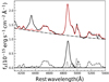 |
Fig. 1. Example of the spectral decomposition of PKS 1510-089. The rest-frame spectrum (black), best-fit model (red), and decomposed AGN power-law component (dashed-dot) are shown along with the Fe II emission (dashed), broad Hβ (solid), and narrow Hβ and [O III] (dotted). |
To minimize any systematic uncertainty due to the decompositions of broad and narrow Hβ components, the total (broad + narrow) Hβ best-fit model was used to estimate Hβ line flux. The Hγ emission line complex consists of broad and narrow Hγ and [O III] λ4363 lines. Since Hγ is much weaker than Hβ, the spectral decomposition is difficult to perform, especially for low S/N spectra. Therefore, instead of modeling the Hγ complex, emission line flux was directly integrated using the best-fit continuum (AGN power-law and Fe II) subtracted spectra. Furthermore, due to low S/N in some epochs and blending with [O III] λ4959, Hβ line wings are not well constrained. Therefore, to minimize any systematic uncertainty in spectral decomposition, the Hβ and Hγ line fluxes were integrated within 4800−4930 Å and 4290−4410 Å, respectively, to avoid the line wings.
Uncertainties in the spectral model parameters (e.g., flux, FWHM, α) were estimated using a Monte Carlo simulation. For each observed spectrum, 100 mock spectra were generated, adding Gaussian random deviates of zero mean and the associated observed flux uncertainty of sigma. Then the same spectral decomposition method was repeated on the mock spectra, as was done for the observed spectrum. The distribution of each parameter from the 100 mock spectra for each original spectrum allowed me to calculate 1σ (68%) dispersion, which I considered the measurement uncertainty of that parameter.
The final analysis was performed on 271 spectra; 70 spectra with poor continuum fitting and low S/N were excluded. The final 5100 Å, Hβ, and Hγ spectroscopic light curves are shown in Fig. 2 and given in Table 1. The variation of the optical spectral index with time is shown. The γ-ray and radio 15 GHz light curves are also shown in Fig. 2.
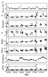 |
Fig. 2. Light curves of PKS 1510-089. From top to bottom: variation of γ ray, V-band, 5100 Å continuum, spectral index, Hβ, Hγ, radio, and non-thermal dominance (NTD; see text) with times. The unit of γ-ray flux is photons s−1 cm−2, f5100 is 10−15 erg s−1 cm−2 Å−1, emission line flux is 10−15 erg s−1 cm−2, and radio flux is Jy. The section between MJD = 55 000−57 100 (window A) of the spectroscopic light curves used in the time series analysis is represented by the vertical lines. The dotted line in the spectroscopic light curve is a linear fit to the data for detrending. Two horizontal lines at NTD = 1 and 2 are shown in the lower panel. |
Spectroscopic data.
3.2. Variability
In order to characterize the flux variation in different wavelengths, the fractional root-mean-square (rms) variability amplitude was calculated following Rodríguez-Pascual et al. (1997):
 (1)
(1)
where σ2 is the variance, ⟨δ2⟩ is the mean square error, and ⟨f⟩ is the arithmetic mean of the light curves. The ratio of maximum to minimum flux variation (Rmax) was also calculated for photometric and spectroscopic light curves. The values are given in Table 2. The source shows strong variations in all bands from γ ray to radio. Optical photometry and 5100 Å spectroscopic light curves also show strong variation. Noteworthy is the correlation of flux variation in optical and γ-ray bands. There are two strong peaks at Modified Julian Date (MJD) = 54 900 and 57 150, where the optical flux shows correlated variation with γ rays; however, emission lines do not show any correlated peaks, suggesting that PKS 1510-089 has a significant non-thermal synchrotron contribution.
Variability statistics.
To determine if the continuum variability of PKS 1510-089 is dominated by the accretion disk (thermal contribution) or the jet (non-thermal synchrotron contribution), the non-thermal dominance (NTD) parameter (Shaw et al. 2012) was calculated following Patino-Alvarez et al. (2016):
 (2)
(2)
where Lo and Lp are the observed continuum luminosity and predicted disk continuum luminosity estimated from the broad emission line, respectively. The observed continuum luminosity of radio-loud sources is a combination of luminosity emitted from the accretion disk (Ld) and the jet (Lj). Therefore, if the thermal emission from the disk is only responsible for ionizing the broad line clouds, then Lp = Ld and NTD = 1 + Lj/Ld. If the continuum is only due to the thermal contribution from the disk, then NTD = 1; however, if the jet also contributes to the continuum luminosity, then NTD > 1. In the case of jet contribution greater than disk contribution, NTD can be larger than 2. To estimate Lp, the correlation of L(Hβ) − L5100 (orthogonal least square) obtained by Rakshit et al. (2020) for non-blazars SDSS DR14 quasars and the L(Hβ) estimated in this work were used. The variation of NTD with time is shown in the last panel of Fig. 2. I note the following points: (1) The NTD varies between 1 and 2 most of the time, suggesting that the non-thermal emission from the jet contributes to the continuum variation, and thermal disk contribution dominates over the jet contribution in the continuum variation. (2) At a few instants, MJD = 54 900 and 57 150, the NTD shows strong spikes, which are correlated with the flaring event in the γ-ray light curve, increasing up to 5 and 7, respectively.
The correlation between the continuum and emission line luminosity of PKS 1510 was studied. In Fig. 3, Hβ luminosity (upper panel) and NTD (bottom panel) are plotted against 5100 Å continuum luminosity. The NTD gradually increases from 1 to 7 with L5100; however, it remains < 2 until log L5100 ∼ 45.6 and increases rapidly for log L5100 > 45.6, reaching NTD ∼7 for the maximum luminosity of log L5100 ∼ 46. A positive (though weak) correlation between L(Hβ) and L5100 is found, with a Spearman correlation coefficient (rs) of 0.39 and a p-value of no-correlation of 10−11. This correlation becomes strong with rs = 0.71 (p-value of 10−35), when sources with NTD < 2 (dotted line) are considered.
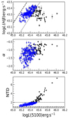 |
Fig. 3. Correlation of Hβ line luminosity (upper panel), optical spectral index (middle panel), and NTD (bottom panel) with L5100 during the monitoring period. The empty squares are the epochs with NTD < 2, while filled circles are those with NTD ≥ 2. The dashed and dotted lines represent NTD = 1 and 2, respectively. |
The spectral slope α (fλ ∝ λα) with L5100 is plotted in the middle panel of Fig. 3. The value of α increases with luminosity. For high luminosity log L5100 > 45.6, α is saturated and no correlation is found with brightness. Those epochs have NTD < 2. The median value of α is −1.19 ± 0.31. A positive correlation in the α − log L5100 relation is found with rs = 0.43 and a p-value of 10−13. Therefore, a “redder when brighter” (RWB) trend is observed in PKS 1510, indicating the presence of an accretion disk in the continuum (e.g., Gu et al. 2006; Nalewajko et al. 2019).
3.3. Time delay measurement
As found in the previous section, the optical continuum light curve of PKS 1510-089 has a non-thermal contribution, which is dominant at some epochs where the γ-ray light curve shows flare. However, broad emission line clouds do not respond to this variation. Therefore, to estimate the time delay between the continuum and emission line variation, a part of the light curve between MJD = 55 000−57 100 was used, denoted by the vertical line (hereafter “window A”).
The spectroscopic light curve of PKS 1510 shows a long-term trend. Such trends, which are not due to the reverberation variation (see Welsh 1999), have been reported in previous RM studies (e.g., Denney et al. 2010; Zhang et al. 2019). Welsh (1999) suggested fitting a low-order (at least linear) polynomial to the light curve and subtracting it from the light curve (i.e., detrending) to improve the cross-correlation results. Therefore, each spectroscopic light curve was detrended prior to the cross-correlation analysis. The linear fits to the f5100, f(Hβ), and f(Hγ;) light curves are indicated in Fig. 2 by the dashed line and the detrended spectroscopic light curves are shown in Fig. 4.
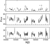 |
Fig. 4. Detrended spectroscopic light curves used in the time delay analysis. From top to bottom: f5100 continuum and Hβ and Hγ line light curves. The units are 10−15 erg s−1 cm−2 Å−1 for f5100 and 10−15 erg s−1 cm−2 for the line light curves. The point above 2 × 10⁻¹⁵ erg s−1 in the f5100 light curve is excluded from the time delay analysis. |
3.3.1. Cross-correlation analysis
The cross-correlation technique (Gaskell & Peterson 1987; White & Peterson 1994; Peterson et al. 2004) was used to measure the time delay. The interpolated cross-correlation function (ICCF) was calculated following the description in Peterson et al. (2004). First, the cross-correlation function (CCF) was calculated with the interpolated continuum light curve while keeping the line light curve unchanged. Then the CCF was re-calculated with the interpolated line light curve while keeping the continuum light curve unchanged. The average of the two CCFs provided the final ICCF. Additionally, the discrete correlation function (DCF) was measured following Edelson & Krolik (1988). The centroid of the CCF (τcent) was calculated using the points at 80% of the CCF peak.
To estimate the uncertainty in τcent, the flux randomization and random subset sampling (FR-RSS) method was used (Peterson et al. 1998, 2004). This was done using Monte Carlo realizations of the light curves. First, a mock light curve was created, adding Gaussian noise based on the associated flux uncertainty. Second, the same number of points as in the original light curve were randomly selected; if one epoch was selected n times, the uncertainty of the flux was reduced by n1/2. A total of 5000 mock light curves were generated and τcent was estimated the same way as for the original light curve. The median of the τcent distribution was taken as the final τcent and its upper and lower uncertainties were calculated such that 15.87% of the realizations fall above the range of uncertainties and 15.87% fall below.
The ICCF and DCF between f5100 and the Hβ and Hγ emission line light curves are shown in Fig. 5, both before and after detrending. In Table 3, the results of the cross-correlation analysis are given. Both the ICCF and DCF methods show consistent results. First, an RM lag is clearly seen from the cross-correlation analysis for the Hβ and Hγ lines both before and after detrending, as the highest significant peak is at the same position and remains unchanged. Second, for both the Hβ and Hγ light curves, the peak of the CCF before detrending is much broader or flatter than that after detrending, although the maximum correlation coefficient (rmax) is slightly higher in the former. Since the CCF after detrending is much narrower and the estimated lags are well constrained, the detrend lag measurement was therefore adopted for further analysis.
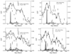 |
Fig. 5. Cross-correlation analysis of f5100 vs. Hβ (top panels) and Hγ (bottom panels) light curves before (left-hand panel) and after detrending (right-hand panel). The ICCF (line) and DCF (points) are shown. The centroid probability distribution from ICCF (filled histogram) and DCF (hatched histogram), along with smooth kernel density (solid and dashed lines, respectively), are also shown. |
Time delay analysis results.
3.3.2. The von Neumann and Bartels estimators
Chelouche et al. (2017) introduced a method to measure time lag based on the regularity or randomness of data. This method requires neither interpolation or binning, nor the stochastic modeling of the light curves. They found that the von Neumann mean-square successive-difference estimator (von Neumann 1941) provides better time delay measurements for irregularly sampled time series where the underlying variability process can not be modeled properly. A detailed description of this method is given in Chelouche et al. (2017). To estimate the time delay between detrended f5100 and the line light curves of PKS 1510, a publicly available python code3 for an optimized von Neumann estimator is used. The time delay distribution obtained from the von Neumann method after a Monte Carlo simulation of FR-RSS, as done for the CCF analysis, is shown in the upper panels of Fig. 6. Both Hβ and Hγ show strong peaks at ∼60 days; however, two additional peaks at around 200 and 300 days are also present. A modification of the von Neumann estimator is the Bartels estimator (Bartels 1982), which can also be used to measure time delay based on the regularity or randomness of data. The time delay distribution based on the Bartels estimator is shown in the lower panels of Fig. 6. Unlike the von Neumann estimator, the Bartels estimator shows a single prominent peak in the distribution. The peaks at around 200 days are absent for both the Hβ and Hγ light curves, and the peaks at 300 days are insignificant compared to the prominent peak at around 60 days. Lag results are given in Table 3.
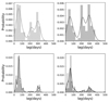 |
Fig. 6. Probability distribution of the observed frame time lag based on the von Neumann estimator (top panels) and the Bartels estimator (bottom panels) for Hβ (left) and Hγ (right). |
3.3.3. JAVELIN
Time delay was also measured by modeling the continuum and line light curves using the JAVELIN code developed by Zu et al. (2011, 2013). JAVELIN first models the driving continuum light curve using a damped random walk (DRW) process (e.g., Kelly et al. 2009) with two parameters: amplitude and time scale of variability. The emission line light curve is a shifted, scaled, and smoothed version of the continuum light curve. JAVELIN then uses a Markov chain Monte Carlo (MCMC) approach to maximize the likelihood of simultaneously modeling the continuum and line light curves. In Fig. 7, the probability distribution of the observed frame lag is plotted in the left-hand panel, as computed by JAVELIN when a lag search is allowed between 0 and 500 days (as was done for the CCF and von Neumann cases). JAVELIN shows prominent peaks at ∼200 and ∼250 days for both Hβ and Hγ. The peaks around ∼60 days, which are found using the ICCF, von Neumann, and Bartels methods, are not visible. To find any peak at a lower lag, JAVELIN was allowed to search for lags between 0 and 180 days by refitting the light curves. The resultant lag probability distribution is shown in the right-hand panels of Fig. 7. In this case, a prominent peak at ∼70 days is found for both the Hβ and Hγ light curves. Time delays obtained from JAVELIN are given in Table 3.
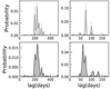 |
Fig. 7. Probability distribution of observed frame lag computed by JAVELIN when lag search is allowed between 0 and 500 (left-hand panels) and 0–180 days (right-hand panels) for Hβ (upper panels) and Hγ (lower panels). |
3.3.4. The χ2-minimization method
Czerny et al. (2013) find that χ2-minimization is a useful method to measure time lag. Therefore, to calculate time lag, χ2-minimization was also applied. First, the mean values were subtracted from the light curves and then normalized by their corresponding standard deviation. The continuum light curve was then linearly interpolated to the emission line light curve and the degree of similarity was calculated by time-shifting the line light curve using the χ2-minimization method. The time lag at which χ2 shows the minimum was considered as the most likely time lag. The final time lag and its uncertainty were calculated using the FR-RSS method, as done in the CCF analysis, for 5000 iterations. The lag probability distribution obtained from χ2-minimization is shown in Fig. 8 and lag values are given in Table 3. The distribution shows a strong peak at ∼60 days for both Hβ and Hγ. Although a small peak at ∼300 days can be found for Hγ, no such peak is found for Hβ.
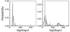 |
Fig. 8. Probability distribution of observed frame lag computed based on the χ2 minimization method. |
The above methods strongly suggest a time lag of ∼60 days between the continuum and the Hβ light curve. To visually check the consistency of the measured lag, the f5100 light curve along with the Hβ light curve back-shifted by 60 days are plotted in Fig. 9. The continuum and back-shifted line light curves match well. Therefore, I adopted the lag of  days obtained by the ICCF method after detrending as the best lag measurement for PKS 1510.
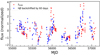 |
Fig. 9. Normalized f5100 light curve plotted along with the Hβ light curve back-shifted by 60 days. |
3.4. Line width and black hole mass
The mean and rms spectra were constructed from the nightly spectrum observed in window A following Rakshit et al. (2019). The mean spectrum is
 (3)
(3)
Here, fi(λ) is the ith spectrum. The rms spectrum is
![Mathematical equation: $$ \begin{aligned} \Delta (\lambda ) =\sqrt{\left[ \frac{1}{N-1} \sum _{i=1}^{N} \left[f_i (\lambda ) - \langle f(\lambda )\rangle \right]^2 \right]}, \end{aligned} $$](/articles/aa/full_html/2020/10/aa38324-20/aa38324-20-eq27.gif) (4)
(4)
where the integration runs from 1 to the total number of spectra (N). The mean and rms spectra are shown in Fig. 10. The rms spectrum clearly shows variations in both the Hβ and Hγ lines.
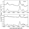 |
Fig. 10. Mean and rms spectra of PKS 1510-089. Top panel: standard mean spectrum (solid line) and a mean spectrum constructed after subtracting the power-law and Fe II (dashed line). Bottom: same as the top panel but for the rms spectrum. |
The FWHM and line dispersion (second moment, σline) were measured from the mean and rms spectra constructed from the nightly spectrum after subtracting the power-law and Fe II component. The FWHM was calculated using the methodology described in Peterson et al. (2004). To measure σline, the flux weighted line center was first determined as follows:
 (5)
(5)
and then the line dispersion as
 (6)
(6)
where fλ is the mean or the rms spectra. The endpoints of the integrations were selected visually to be 4800−4930 Å for Hβ. To estimate uncertainty in the line width measurements, the Monte Carlo bootstrap method (Peterson et al. 2004) was used. For each realization, N spectra were randomly selected from a set of N spectra without replacement and the line width was calculated from the mean and rms spectra. In each realization, the endpoints of the integration window were randomly varied within ±10 Å from the initial selections. A total of 5000 realizations were performed, providing a distribution of FWHM and σline. The median of the distribution was taken as the final line width and the standard deviation of the distribution was considered to be the measurement uncertainty. The final line width measurements, after correcting for the instrumental resolution of FWHM ∼1150 km s−1 (see Zhang et al. 2019), are given in Table 4.
Rest-frame resolution-corrected line width and black hole mass measurements from mean and rms spectra created from the nightly spectrum after subtracting the power-law and Fe II component.
The black hole mass of PKS 1510-089 was determined using the virial relation as follows:
 (7)
(7)
Here, f is the virial factor, RBLR = cτ is the BLR size in the rest-frame, and ΔV is the velocity width of the broad emission line.
The black hole mass was determined using an Hβ lag of  days, which corresponds to a rest-frame BLR size of
  light-days. Both the resolution-corrected FWHM and σline measured from the mean and rms spectra of Hβ were used as ΔV. A value of f = 4.47 (1.12) was adopted when σline (FWHM) is considered as ΔV (Woo et al. 2015); however, I note that FWHM is a non-linear function of σline (e.g., Peterson 2014; Bonta et al. 2020). Finally, four different black hole masses were determined based on the four different choices of line widths (see Table 4). The black hole masses and their uncertainties are calculated based on the error propagation method and given in Table 4. I note that σline is less sensitive to the line peak, and that FWHM is less sensitive to the line wing; therefore, black hole masses based on the σline are widely adopted as the best mass measurement (e.g., Peterson et al. 2004; Peterson 2014). Therefore,
  of PKS 1510-089 from σline of rms spectrum was adopted in this work.
4. Discussion
4.1. Impact of seasonal gaps on lag measurement
The monitoring of PKS 1510 is strongly affected by seasonal gaps of about six months, which are due to its low declination. Therefore, any lag close to the average seasonal gaps of ∼180 days will be difficult to measure because the emission-line response to the continuum variations occurs when the source is unobservable. The measured monochromatic luminosity of PKS 1510-089 from the mean spectra is L5100 = 2.39 × 1045 ers s−1. Using the RBLR − L5100 relation of a radio-quiet AGN sample presented by Bentz et al. (2013), an expected BLR size of ∼182 days and an observed frame lag of 248 days are obtained for PKS 1510. As the expected lag is closer to the seasonal gaps, the impact of seasonal gaps on the lag measurement was investigated via the construction of mock light curves. For this purpose, a mock continuum light curve was constructed using the DRW model implemented in JAVELIN, which has a similar characteristic as the observed continuum light curve. Then mock line light curves with time delays of 70 and 200 days were constructed. To mimic the observed light curves, mock light curves were down-sampled to have the same time sampling, and therefore the same time axis, as the observed light curves. To recover the input time delay, time series analysis methods, as described in Sect. 3.3, were used on the mock data sets.
The results are shown in Fig. A.1 and are given in Table A.1 of the appendix. The results show that the ICCF, DCF, von Neumann, and Bartels methods recover an input lag of 70 days, and the measurements are not affected by the seasonal gaps and time sampling. I note that the rmax obtained by ICCF and DCF is ∼0.6, which is similar to that obtained in the case of the observed light curve (see Fig. 5). Interestingly, JAVELIN results are affected by seasonal gaps, as they show a primary peak at ∼160 days. Due to the same reason, JAVELIN finds a lag at ∼200 days for the observed light curve of PKS 1510 when the lag search is allowed between 0 and 500 days (see Sect. 3.3.3). A secondary peak at ∼70 days, which is the same as the input lag, is also found in the JAVELIN lag probability distribution, as shown in Fig. A.1. For an input lag of 200 days, both the ICCF and DCF show no correlation between the mock continuum and the line light curve due to the seasonal gaps; therefore, they do not allow me to estimate the lag. However, the von Neumann, Bartels, and JAVELIN methods successfully recover the input time lag of 200 days, albeit with larger uncertainty. Therefore, the uses of various time series analysis methods allow me to recover a lag of ∼200 days, although the light curves are affected by the seasonal gaps and a lag of ∼70 days can be well-constrained with lower uncertainty. The above simulations suggest any lag close to ∼200 days is unlikely for PKS 1510, while a lag of ∼60 days is most likely.
4.2. Size-luminosity relation
The quasar PKS 1510-089 is a radio-loud source with strong γ-ray activity. From Fig. 3, it is clear that the measured L5100 is a combination of non-thermal synchrotron emission from the jet and thermal emission from the accretion disk. Hence, L5100 measurement is strongly affected by the non-thermal emission. In Fig. 11, the BLR size of PKS 1510-089 is plotted against L5100, along with the previous reverberation mapped objects from the literature (e.g., Bentz et al. 2013; Du et al. 2016b; Grier et al. 2017; De Rosa et al. 2018; Rakshit et al. 2019); PKS 1510-089 is found to deviate from the RBLR − L5100 relation of Bentz et al. (2013). However, this is not surprising considering the fact that previous studies of high-accreting and strong Fe II-emitting AGNs show significant deviation from the size-luminosity relation (Du et al. 2016a, 2018). This could be due to the complex radiation field and BLR geometry in high-accreting AGNs, which may have slim accretion disks. The strong self-shadowing effects on the slim accretion disks may produce a highly anisotropic radiation field, which, depending on the accretion rate, may lead to two dynamically distinct regions of the BLR (Wang et al. 2014). Du & Wang (2019) find that the RFeII, (i.e., the flux ratio of Fe II to Hβ) is the main driver of the shortened lag obtained in the high-accreting AGNs. They provide a new scaling relation, which includes RFeII. Using the mean RFeII of 0.52 ± 0.09 found in PKS 1510-089, the expected lag is about ∼122 days, which is lower than what is expected from the Bentz et al. (2013) relation but still a factor of three larger than the measured lag. Several authors (Celotti et al. 1997; Abdo et al. 2010a; Nalewajko et al. 2012) have estimated the disk bolometric luminosity (Ldisk) of PKS 1510-089, which is in the range of 3−7 × 1045 erg s−1. This, based on a simple scaling relation of  cm (Ghisellini & Tavecchio 2009), provides RBLR = 66−102 light-days. Our estimated rest-frame RBLR is slightly lower than the above values.
Li et al. (2020) studied a well-known FSRQ, 3C273, and find that the optical continuum has two components of emissions, one from the accretion disk and another from the jet. The jet contribution is found to be 10–40% of the total optical emissions. Whiting et al. (2001) showed that the synchrotron radiation from the jet contributes to the optical band, thereby increasing the total optical continuum flux. However, due to beaming, this synchrotron component does not contribute to ionizing the emission line clouds. Figure 2 shows strong γ-ray activity in PKS 1510-089 at MJD ≃ 54 900 and 57 150. Although the light curve when PKS 1510-089 is mostly in a quiescent state is analyzed in this work, a non-thermal contribution from the jet is always present. To have a rough estimation of thermal contribution in L5100, the median of the NTD was calculated in the quiescent state (window A). It is found to be  , indicating that the disk contribution to the measured L5100 is about 60%.
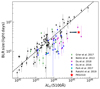 |
Fig. 11. PKS 1510-089 in the BLR size vs. L5100 relation of AGNs. The best-fit relation of Bentz et al. (2013) is shown along with various RM results from the literature. The arrow indicates that the accretion disk contribution to the measured L5100 of PKS 1510-089 could be much lower. |
This contribution can also be roughly estimated from the broad-band SED. Prince et al. (2019) studied the broad-band SED of PKS 1510-089 in several active and quiescent states in 2015 (MJD = 57 000−57 350). They modeled the broad-band SED using a time-dependent two-zone emission model and estimated the synchrotron, synchrotron self-Compton (SSC), and inverse-Compton emission. They estimated the disk contribution at 5100 Å to the total flux during one quiescent state (Q2 between MJD = 57 180−57 208; see Fig. 3 of Prince et al. 2019). The disk contribution is found to be ∼44% of the total flux at 5100 Å, lower than that estimated from the NTD but consistent within the margin of error. If the measured L5100 is corrected assuming the disk contribution is 60% (based on the NTD calculation), the corrected L5100 is 1.43 × 1045 ers s−1. In fact, using the mean Hβ line luminosity of 2.04 × 1043 erg s−1 and the scaling relation of L(Hβ) − L(5100) for radio quiet AGNs from Liu et al. (2006), L5100 is found to be 1.40 × 1045 ers s−1. Therefore, the measured L5100 of PKS 1510-089 is an upper-limit, as it is significantly affected by the non-thermal contribution from the jet. Furthermore, the host galaxy also contributes to the measured L5100. Therefore, the measured L5100 is an upper limit and the actual position of PKS 1510-089 in the size-luminosity diagram is highly uncertain.
4.3. Black hole mass measurement
Since PKS 1510-089 is a well-studied object, several authors have reported its black hole mass based on single-epoch spectrum, variability time scale, accretion disk modeling, etc. Here, the mass measurement is compared with those in the literature. The estimated black hole of PKS 1510-089 ranges from 4.19−7.02 × 10⁷M⊙, depending on the choice of the line width and line profile used. The bolometric luminosity is found to be 21.51 × 1045 erg s−1, based on the measured L5100 from the mean spectrum using LBOL = 9 × L5100 (Kaspi et al. 2000). The Eddington ratio (λEDD) is 2.98, estimated using LEDD = 1.26 × 1038MBH and the black hole mass based on the σline of rms spectrum. However, using the corrected L5100 due to jet contribution, λEDD = 1.78 is found, suggesting that PKS 1510-089 is accreting at a mildly super-Eddington rate. This value is similar to the λEDD = 2.4 found for another FSRQ, 3C273 (Zhang et al. 2019).
Oshlack et al. (2002), using single-epoch spectrum, estimated the black hole mass of PKS 1510-089 to be 3.86 × 10⁸M⊙. Similarly, Xie et al. (2005), based on the minimum time scale of variability and single-epoch spectrum, estimated black hole masses of MBH = 1.1 × 10⁸M⊙ and 1.6 × 10⁸M⊙, respectively (see also Liu et al. 2006; Park & Trippe 2017). I note that single-epoch black hole masses depend on the choice of the scaling relation, which shows significant scatter; highly accreting sources especially show larger offset from the RBLR − L5100 relation. The choice of the line width measurement, FWHM or σline, also affects the single-epoch mass measurement. Reverberation mapping studies of AGNs, in which multiple emission lines have been observed, suggest σline is a better measure for black hole mass than FWHM (Peterson et al. 2004). Moreover, an rms profile, which can only be constructed from multi-epoch spectra, should be used to estimate black hole masses, as it shows the variable component of the emission line; contaminating features – such as constant host-galaxy contribution and narrow-line components, which are present in the single-epoch spectrum or in the mean spectrum – disappear in the rms spectrum (see Peterson 2014). Using UV data, Abdo et al. (2010a) estimated a black hole mass for PKS 1510-089 as MBH = 5.4 × 10⁸M⊙. On the other hand, Castignani et al. (2017), using the Shakura & Sunyaev (1973) model, estimated a black hole mass of 2.4 × 10⁸M⊙. Therefore, a large range of black hole masses, 1−9 × 10⁸M⊙, for PKS 1510-089 has been reported in the literature. Considering the typical uncertainty of ∼0.5 dex in the mass measurement (Shen 2013), the estimated black hole mass of PKS 1510-089 is smaller by a factor of 2−4 than the values reported in the literature.
5. Conclusion
The optical spectroscopic RM results of PKS 1510-089 from an ∼8.5-year long monitoring campaign carried out at Steward Observatory from December 2008 to June 2017 are presented. The nightly spectrum shows the presence of broad Hβ, Hγ, and Fe II emission overlying on a blue continuum. During the monitoring program, both the optical continuum and Hβ line show strong variation with fractional rms variations (Fvar) of: 37.30 ± 0.06% for f5100; 11.88 ± 0.29% for Hβ; and 9.61 ± 0.71% for Hγ light curves. With the increase of L5100 from 1045.2 to 1045.6 erg s−1, the Hβ line luminosity increases from 1043.2 to 1043.5 erg s−1 but decreases as L5100 > 1045.6 erg s−1. Although the optical continuum is dominated by thermal radiation from the accretion disk, non-thermal synchrotron contribution from the jet is clearly present, which does not contribute to ionizing the emission line clouds. From cross-correlation analysis, the Hβ and Hγ lags are found to be  days and
  days, respectively. This corresponds to a rest-frame BLR size of
  light-days for Hβ and
  light-days for Hγ. Using a scale factor of 4.47 and the σline from the rms spectrum, which is constructed from the nightly spectrum after subtracting the power-law and Fe II, the black hole mass of PKS 1510-089 is found to be
  .
.
Acknowledgments
Many thanks go to the referee for comments and suggestions that helped to improve the quality of the manuscript. Thanks to Prince Raj for providing their SED model component of PKS1510-089 and Neha Sharma for carefully reading the manuscript. This publication makes use of data products from the Fermi Gamma-ray Space Telescope and accessed from the Fermi Science Support Center. Data from the Steward Observatory spectropolarimetric monitoring project were used. This program is supported by Fermi Guest Investigator grants NNX08AW56G, NNX09AU10G, NNX12AO93G, and NNX15AU81G. This research has made use of data from the OVRO 40-m monitoring program (Richards et al. 2011) which is supported in part by NASA grants NNX08AW31G, NNX11A043G, and NNX14AQ89G and NSF grants AST-0808050 and AST-1109911
References
- Abdo, A. A., Ackermann, M., Ajello, M., et al. 2009, ApJ, 700, 597 [NASA ADS] [CrossRef] [Google Scholar]
- Abdo, A. A., Ackermann, M., Agudo, I., et al. 2010a, ApJ, 721, 1425 [NASA ADS] [CrossRef] [Google Scholar]
- Abdo, A. A., Ackermann, M., Agudo, I., et al. 2010b, ApJ, 716, 30 [NASA ADS] [CrossRef] [Google Scholar]
- Bach, U., Raiteri, C. M., Villata, M., et al. 2007, A&A, 464, 175 [NASA ADS] [CrossRef] [EDP Sciences] [Google Scholar]
- Bartels, R. 1982, J. Am. Stat. Assoc., 77, 40 [CrossRef] [Google Scholar]
- Beaklini, P. P. B., Dominici, T. P., & Abraham, Z. 2017, A&A, 606, A87 [NASA ADS] [CrossRef] [EDP Sciences] [Google Scholar]
- Bentz, M. C., Denney, K. D., Grier, C. J., et al. 2013, ApJ, 767, 149 [NASA ADS] [CrossRef] [Google Scholar]
- Bentz, M. C., Peterson, B. M., Netzer, H., Pogge, R. W., & Vestergaard, M. 2009, ApJ, 697, 160 [Google Scholar]
- Blandford, R. D., & McKee, C. F. 1982, ApJ, 255, 419 [NASA ADS] [CrossRef] [EDP Sciences] [Google Scholar]
- Bonta, E. D., Peterson, B. M., Bentz, M. C., et al. 2020, ApJ, submitted [arXiv:2007.02963] [Google Scholar]
- Cardelli, J. A., Clayton, G. C., & Mathis, J. S. 1989, ApJ, 345, 245 [NASA ADS] [CrossRef] [Google Scholar]
- Castignani, G., Pian, E., Belloni, T. M., et al. 2017, A&A, 601, A30 [NASA ADS] [CrossRef] [EDP Sciences] [Google Scholar]
- Celotti, A., Padovani, P., & Ghisellini, G. 1997, MNRAS, 286, 415 [NASA ADS] [CrossRef] [EDP Sciences] [Google Scholar]
- Chelouche, D., Pozo-Nuñez, F., & Zucker, S. 2017, ApJ, 844, 146 [CrossRef] [Google Scholar]
- Cho, H., Woo, J.-H., Hodges-Kluck, E., et al. 2020, ApJ, 892, 93 [NASA ADS] [CrossRef] [Google Scholar]
- Czerny, B., Hryniewicz, K., Maity, I., et al. 2013, A&A, 556, A97 [NASA ADS] [CrossRef] [EDP Sciences] [Google Scholar]
- De Rosa, G., Fausnaugh, M. M., Grier, C. J., et al. 2018, ApJ, 866, 133 [NASA ADS] [CrossRef] [Google Scholar]
- Denney, K. D., Peterson, B. M., Pogge, R. W., et al. 2010, ApJ, 721, 715 [NASA ADS] [CrossRef] [Google Scholar]
- Du, P., & Wang, J.-M. 2019, ApJ, 886, 42 [NASA ADS] [CrossRef] [Google Scholar]
- Du, P., Lu, K.-X., Zhang, Z.-X., et al. 2016a, ApJ, 825, 126 [NASA ADS] [CrossRef] [Google Scholar]
- Du, P., Lu, K.-X., Hu, C., et al. 2016b, ApJ, 820, 27 [NASA ADS] [CrossRef] [Google Scholar]
- Du, P., Zhang, Z.-X., Wang, K., et al. 2018, ApJ, 856, 6 [NASA ADS] [CrossRef] [Google Scholar]
- Edelson, R. A., & Krolik, J. H. 1988, ApJ, 333, 646 [NASA ADS] [CrossRef] [Google Scholar]
- Gaskell, C. M., & Peterson, B. M. 1987, ApJS, 65, 1 [NASA ADS] [CrossRef] [Google Scholar]
- Ghisellini, G., & Tavecchio, F. 2009, MNRAS, 397, 985 [NASA ADS] [CrossRef] [Google Scholar]
- Grier, C. J., Trump, J. R., Shen, Y., et al. 2017, ApJ, 851, 21 [CrossRef] [Google Scholar]
- Gu, M. F., Lee, C. U., Pak, S., Yim, H. S., & Fletcher, A. B. 2006, A&A, 450, 39 [NASA ADS] [CrossRef] [EDP Sciences] [Google Scholar]
- H.E.S.S. Collaboration (Abramowski, A., et al.) 2013, A&A, 554, A107 [NASA ADS] [CrossRef] [EDP Sciences] [Google Scholar]
- Kaspi, S., Smith, P. S., Netzer, H., et al. 2000, ApJ, 533, 631 [NASA ADS] [CrossRef] [Google Scholar]
- Kelly, B. C., Bechtold, J., & Siemiginowska, A. 2009, ApJ, 698, 895 [Google Scholar]
- Kormendy, J., & Ho, L. C. 2013, ARA&A, 51, 511 [Google Scholar]
- Kovačević, J., Popović, L. Č., & Dimitrijević, M. S. 2010, ApJS, 189, 15 [NASA ADS] [CrossRef] [Google Scholar]
- Kushwaha, P., Chandra, S., Misra, R., et al. 2016, ApJ, 822, L13 [NASA ADS] [CrossRef] [Google Scholar]
- Li, Y.-R., Zhang, Z.-X., Jin, C., et al. 2020, ApJ, 897, 18 [CrossRef] [Google Scholar]
- Liu, Y., Jiang, D. R., & Gu, M. F. 2006, ApJ, 637, 669 [NASA ADS] [CrossRef] [Google Scholar]
- Malkan, M. A., & Moore, R. L. 1986, ApJ, 300, 216 [NASA ADS] [CrossRef] [Google Scholar]
- Markwardt, C. B. 2009, in Astronomical Data Analysis Software and Systems XVIII, eds. D. A. Bohlender, D. Durand, & P. Dowler, ASP Conf. Ser., 411, 251 [Google Scholar]
- Marscher, A. P., Jorstad, S. G., Larionov, V. M., et al. 2010, ApJ, 710, L126 [NASA ADS] [CrossRef] [Google Scholar]
- Nalewajko, K., Sikora, M., Madejski, G. M., et al. 2012, ApJ, 760, 69 [NASA ADS] [CrossRef] [EDP Sciences] [Google Scholar]
- Nalewajko, K., Gupta, A. C., Liao, M., et al. 2019, A&A, 631, A4 [NASA ADS] [CrossRef] [EDP Sciences] [Google Scholar]
- Orienti, M., Koyama, S., D’Ammando, F., et al. 2013, MNRAS, 428, 2418 [Google Scholar]
- Oshlack, A. Y. K. N., Webster, R. L., & Whiting, M. T. 2002, ApJ, 576, 81 [NASA ADS] [CrossRef] [Google Scholar]
- Park, J., & Trippe, S. 2017, ApJ, 834, 157 [CrossRef] [Google Scholar]
- Park, S., Woo, J.-H., Romero-Colmenero, E., et al. 2017a, ApJ, 847, 125 [NASA ADS] [CrossRef] [Google Scholar]
- Park, D., Barth, A. J., Woo, J.-H., et al. 2017b, ApJ, 839, 93 [NASA ADS] [CrossRef] [Google Scholar]
- Patino-Alvarez, V. M., Torrealba, J., Chavushyan, V., et al. 2016, Front. Astron. Space Sci., 3, 19 [NASA ADS] [CrossRef] [Google Scholar]
- Peterson, B. M. 1993, PASP, 105, 247 [NASA ADS] [CrossRef] [Google Scholar]
- Peterson, B. M. 2014, Space Sci. Rev., 183, 253 [NASA ADS] [CrossRef] [Google Scholar]
- Peterson, B. M., Wanders, I., Horne, K., et al. 1998, PASP, 110, 660 [NASA ADS] [CrossRef] [Google Scholar]
- Peterson, B. M., Ferrarese, L., Gilbert, K. M., et al. 2004, ApJ, 613, 682 [NASA ADS] [CrossRef] [Google Scholar]
- Prince, R., Gupta, N., & Nalewajko, K. 2019, ApJ, 883, 137 [Google Scholar]
- Rakshit, S., & Woo, J.-H. 2018, ApJ, 865, 5 [NASA ADS] [CrossRef] [Google Scholar]
- Rakshit, S., Woo, J.-H., Gallo, E., et al. 2019, ApJ, 886, 93 [NASA ADS] [CrossRef] [Google Scholar]
- Rakshit, S., Stalin, C. S., & Kotilainen, J. 2020, ApJS, 249, 17 [CrossRef] [Google Scholar]
- Richards, J. L., Max-Moerbeck, W., Pavlidou, V., et al. 2011, ApJS, 194, 29 [Google Scholar]
- Rodríguez-Pascual, P. M., Alloin, D., Clavel, J., et al. 1997, ApJS, 110, 9 [NASA ADS] [CrossRef] [Google Scholar]
- Schlafly, E. F., & Finkbeiner, D. P. 2011, ApJ, 737, 103 [NASA ADS] [CrossRef] [Google Scholar]
- Schmidt, G. D., Stockman, H. S., & Smith, P. S. 1992, ApJ, 398, L57 [NASA ADS] [CrossRef] [Google Scholar]
- Shakura, N. I., & Sunyaev, R. A. 1973, A&A, 500, 33 [NASA ADS] [Google Scholar]
- Shaw, M. S., Romani, R. W., Cotter, G., et al. 2012, ApJ, 748, 49 [CrossRef] [Google Scholar]
- Shen, Y. 2013, Bull. Astron. Soc. India, 41, 61 [NASA ADS] [Google Scholar]
- Shen, Y., Horne, K., Grier, C. J., et al. 2016, ApJ, 818, 30 [NASA ADS] [CrossRef] [Google Scholar]
- Sikora, M., Begelman, M. C., & Rees, M. J. 1994, ApJ, 421, 153 [Google Scholar]
- Smith, P. S., Montiel, E., Rightley, S., et al. 2009, 2009 Fermi Symposium, eConf Proceedings C091122 [arXiv:0912.3621] [Google Scholar]
- Tadhunter, C. N., Morganti, R., di Serego Alighieri, S., Fosbury, R. A. E., & Danziger, I. J. 1993, MNRAS, 263, 999 [NASA ADS] [CrossRef] [Google Scholar]
- Tavecchio, F., Maraschi, L., Ghisellini, G., et al. 2000, ApJ, 543, 535 [Google Scholar]
- Thompson, D. J., Djorgovski, S., & de Carvalho, R. 1990, PASP, 102, 1235 [NASA ADS] [CrossRef] [Google Scholar]
- Urry, C. M., & Padovani, P. 1995, PASP, 107, 803 [NASA ADS] [CrossRef] [Google Scholar]
- von Neumann, J. 1941, Ann. Math. Statist., 12, 367 [CrossRef] [Google Scholar]
- Wandel, A., Peterson, B. M., & Malkan, M. A. 1999, ApJ, 526, 579 [NASA ADS] [CrossRef] [Google Scholar]
- Wang, J.-M., Qiu, J., Du, P., & Ho, L. C. 2014, ApJ, 797, 65 [NASA ADS] [CrossRef] [Google Scholar]
- Welsh, W. F. 1999, PASP, 111, 1347 [Google Scholar]
- White, R. J., & Peterson, B. M. 1994, PASP, 106, 879 [NASA ADS] [CrossRef] [Google Scholar]
- Whiting, M. T., Webster, R. L., & Francis, P. J. 2001, MNRAS, 323, 718 [NASA ADS] [CrossRef] [Google Scholar]
- Woo, J.-H., Yoon, Y., Park, S., Park, D., & Kim, S. C. 2015, ApJ, 801, 38 [NASA ADS] [CrossRef] [Google Scholar]
- Wood, M., Caputo, R., Charles, E., et al. 2017, PoS, ICRC2017, 824 [Google Scholar]
- Xie, G. Z., Liu, H. T., Cha, G. W., et al. 2005, AJ, 130, 2506 [NASA ADS] [CrossRef] [Google Scholar]
- Zajaček, M., Czerny, B., Martinez-Aldama, M. L., et al. 2020, ApJ, 896, 146 [CrossRef] [Google Scholar]
- Zhang, Z.-X., Du, P., Smith, P. S., et al. 2019, ApJ, 876, 49 [NASA ADS] [CrossRef] [Google Scholar]
- Zu, Y., Kochanek, C. S., & Peterson, B. M. 2011, ApJ, 735, 80 [NASA ADS] [CrossRef] [Google Scholar]
- Zu, Y., Kochanek, C. S., Kozłowski, S., & Udalski, A. 2013, ApJ, 765, 106 [NASA ADS] [CrossRef] [Google Scholar]
Appendix A: Time series analysis of simulated light curves
To study the impact of seasonal gaps on the lag measurement, the DRW model implemented in JAVELIN was used to construct a mock continuum light curve that has similar characteristics as the observed f5100 light curve of PKS 1510. Then two mock line light curves were constructed with a lag of 70 and 200 days. The light curves were down-sampled to have the same time sampling as the observed light curves, therefore mimicking the observed time axis. The time series analysis methods (ICCF, DCF, von Neumann, Bartels, and JAVELIN) were then used on the mock continuum and line light curves to recover the input time lag. The results are shown in Fig. A.1 and given in Table A.1.
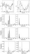 |
Fig. A.1. From top to bottom: lag probability distributions obtained from the CCF (ICCF and DCF), von Neumann, Bartels, and JAVELIN methods for the mock continuum vs. mock line light curve with a delay of 200 days (left) and 70 days (right). The lag probability distribution (histogram), along with the smoothed kernel density distribution, is shown in each panel. |
Time delay analysis results on mock light curves.
All Tables
Rest-frame resolution-corrected line width and black hole mass measurements from mean and rms spectra created from the nightly spectrum after subtracting the power-law and Fe II component.
All Figures
|
Fig. 1. Example of the spectral decomposition of PKS 1510-089. The rest-frame spectrum (black), best-fit model (red), and decomposed AGN power-law component (dashed-dot) are shown along with the Fe II emission (dashed), broad Hβ (solid), and narrow Hβ and [O III] (dotted). |
| In the text | |
|
Fig. 2. Light curves of PKS 1510-089. From top to bottom: variation of γ ray, V-band, 5100 Å continuum, spectral index, Hβ, Hγ, radio, and non-thermal dominance (NTD; see text) with times. The unit of γ-ray flux is photons s−1 cm−2, f5100 is 10−15 erg s−1 cm−2 Å−1, emission line flux is 10−15 erg s−1 cm−2, and radio flux is Jy. The section between MJD = 55 000−57 100 (window A) of the spectroscopic light curves used in the time series analysis is represented by the vertical lines. The dotted line in the spectroscopic light curve is a linear fit to the data for detrending. Two horizontal lines at NTD = 1 and 2 are shown in the lower panel. |
| In the text | |
|
Fig. 3. Correlation of Hβ line luminosity (upper panel), optical spectral index (middle panel), and NTD (bottom panel) with L5100 during the monitoring period. The empty squares are the epochs with NTD < 2, while filled circles are those with NTD ≥ 2. The dashed and dotted lines represent NTD = 1 and 2, respectively. |
| In the text | |
|
Fig. 4. Detrended spectroscopic light curves used in the time delay analysis. From top to bottom: f5100 continuum and Hβ and Hγ line light curves. The units are 10−15 erg s−1 cm−2 Å−1 for f5100 and 10−15 erg s−1 cm−2 for the line light curves. The point above 2 × 10⁻¹⁵ erg s−1 in the f5100 light curve is excluded from the time delay analysis. |
| In the text | |
|
Fig. 5. Cross-correlation analysis of f5100 vs. Hβ (top panels) and Hγ (bottom panels) light curves before (left-hand panel) and after detrending (right-hand panel). The ICCF (line) and DCF (points) are shown. The centroid probability distribution from ICCF (filled histogram) and DCF (hatched histogram), along with smooth kernel density (solid and dashed lines, respectively), are also shown. |
| In the text | |
|
Fig. 6. Probability distribution of the observed frame time lag based on the von Neumann estimator (top panels) and the Bartels estimator (bottom panels) for Hβ (left) and Hγ (right). |
| In the text | |
|
Fig. 7. Probability distribution of observed frame lag computed by JAVELIN when lag search is allowed between 0 and 500 (left-hand panels) and 0–180 days (right-hand panels) for Hβ (upper panels) and Hγ (lower panels). |
| In the text | |
|
Fig. 8. Probability distribution of observed frame lag computed based on the χ2 minimization method. |
| In the text | |
|
Fig. 9. Normalized f5100 light curve plotted along with the Hβ light curve back-shifted by 60 days. |
| In the text | |
|
Fig. 10. Mean and rms spectra of PKS 1510-089. Top panel: standard mean spectrum (solid line) and a mean spectrum constructed after subtracting the power-law and Fe II (dashed line). Bottom: same as the top panel but for the rms spectrum. |
| In the text | |
|
Fig. 11. PKS 1510-089 in the BLR size vs. L5100 relation of AGNs. The best-fit relation of Bentz et al. (2013) is shown along with various RM results from the literature. The arrow indicates that the accretion disk contribution to the measured L5100 of PKS 1510-089 could be much lower. |
| In the text | |
|
Fig. A.1. From top to bottom: lag probability distributions obtained from the CCF (ICCF and DCF), von Neumann, Bartels, and JAVELIN methods for the mock continuum vs. mock line light curve with a delay of 200 days (left) and 70 days (right). The lag probability distribution (histogram), along with the smoothed kernel density distribution, is shown in each panel. |
| In the text | |
Current usage metrics show cumulative count of Article Views (full-text article views including HTML views, PDF and ePub downloads, according to the available data) and Abstracts Views on Vision4Press platform.
Data correspond to usage on the plateform after 2015. The current usage metrics is available 48-96 hours after online publication and is updated daily on week days.
Initial download of the metrics may take a while.