| Issue |
A&A
Volume 640, August 2020
|
|
|---|---|---|
| Article Number | A136 | |
| Number of page(s) | 22 | |
| Section | Planets and planetary systems | |
| DOI | https://doi.org/10.1051/0004-6361/202038101 | |
| Published online | 28 August 2020 | |
Directly imaged exoplanets in reflected starlight: the importance of knowing the planet radius
1
Zentrum für Astronomie und Astrophysik, Technische Universität Berlin,
Hardenbergstrasse 36,
10623
Berlin, Germany
e-mail: o.carriongonzalez@astro.physik.tu-berlin.de; oscar.carrion.gonzalez@gmail.com
2
Deutsches Zentrum für Luft- und Raumfahrt,
Rutherfordstraße 2,
12489
Berlin, Germany
3
Instituto de Astrofísica e Ciências do Espaço, Universidade do Porto, CAUP, Rua das Estrelas,
4150-762
Porto, Portugal
4
Departamento de Física e Astronomia, Faculdade de Ciências, Universidade do Porto, Rua do Campo Alegre,
4169-007
Porto, Portugal
5
Institute of Geological Sciences, Freie Universität Berlin, Malteserstrasse 74-100,
12249
Berlin, Germany
Received:
6
April
2020
Accepted:
12
June
2020
Context. The direct imaging of exoplanets in reflected starlight will represent a major advance in the study of cold and temperate exoplanet atmospheres. Understanding how basic planet and atmospheric properties may affect the measured spectra is key to their interpretation.
Aims. We have investigated the information content in reflected-starlight spectra of exoplanets. We apply our analysis to Barnard’s Star b candidate super-Earth, for which we assume a radius 0.6 times that of Neptune, an atmosphere dominated by H2–He, and a CH4 volume mixing ratio of 5 × 10⁻³. The main conclusions of our study are however planet-independent.
Methods. We set up a model of the exoplanet described by seven parameters including its radius, atmospheric methane abundance, and basic properties of a cloud layer. We generated synthetic spectra at zero phase (full disc illumination) from 500 to 900 nm and a spectral resolution R ~ 125–225. We simulated a measured spectrum with a simplified, wavelength-independent noise model at a signal-to-noise ratio of 10. With a retrieval methodology based on Markov chain Monte Carlo sampling, we analysed which planet and atmosphere parameters can be inferred from the measured spectrum and the theoretical correlations amongst them. We considered limiting cases in which the planet radius is either known or completely unknown, and intermediate cases in which the planet radius is partly constrained.
Results. If the planet radius is known, we can generally discriminate between cloud-free and cloudy atmospheres, and constrain the methane abundance to within two orders of magnitude. If the planet radius is unknown, new correlations between model parameters occur and the accuracy of the retrievals decreases. Without a radius determination, it is challenging to discern whether the planet has clouds, and the estimates on methane abundance degrade. However, we find the planet radius is constrained to within a factor of two for all the cases explored. Having a priori information on the planet radius, even if approximate, helps improve the retrievals.
Conclusions. Reflected-starlight measurements will open a new avenue for characterizing long-period exoplanets, a population that remains poorly studied. For this task to be complete, direct-imaging observations should be accompanied by other techniques. We urge exoplanet detection efforts to extend the population of long-period planets with mass and radius determinations.
Key words: planets and satellites: atmospheres / planets and satellites: gaseous planets / radiative transfer
© ESO 2020
1 Introduction
Upcoming space missions such as the Wide Field Infrared Survey Telescope (WFIRST)1 (Spergel et al. 2013) and mission concepts such as the Large UV Optical Infrared telescope (LUVOIR; Bolcar et al. 2016) or the Habitable Exoplanet Observatory (HabEx; Mennesson et al. 2016) aim to measure the starlight reflected from cold and temperate exoplanets by direct imaging. This offers opportunities to detect and characterize long-period exoplanets, a population that remains substantially unexplored due to current technological biases. Due to their lower equilibrium temperatures, these planets are expected to have very different atmospheric properties from those currently observed in transit.
Characterizing long-period exoplanets will help complete the picture of extrasolar planetary systems and shape the formation and evolution theories that explain their architectures (D’Angelo & Bodenheimer 2013; Fabrycky et al. 2014). The probability that these long-period planets are observed in transit is small, since it decreases with the orbital distance. Furthermore, even if they transit, atmospheric refraction will limit the insight obtained from transmission spectroscopy (García Muñoz et al. 2012; Misra et al. 2014). Hence, direct imaging will be key to analyse these planets.
In preparation for these missions, it is crucial to investigate what information can be extracted from measurements of reflected starlight from spatially unresolved planets. The underlying question is certainly not new, and there is a vast literature examining the diagnostic possibilities of reflected light in general remote sensing applications. For instance, in the framework of Earth observations, Stephens & Heidinger (2000) and Heidinger & Stephens (2000) examined the potential of satellite observations of possibly cloudy views above our planet’s surface. They concluded that six main parameters affect a reflected-light spectrum, namely: the optical thickness of the cloud, its geometrical thickness, the pressure level of the cloud top, the scattering phase function and single-scattering albedo of the cloud particles, and the surface reflectivity.
The interpretation of direct-imaging observations of exoplanets in reflected starlight will rely on essentially the same physical principles. Although the above space missions are still years away, there is already significant interest in understanding their prospective scientific output (see e.g. Cahoy et al. 2010; Greco & Burrows 2015; Lupu et al. 2016; Robinson et al. 2016; Nayak et al. 2017; Batalha et al. 2018; Feng et al. 2018; Guimond & Cowan 2018; Damiano & Hu 2019; Hu 2019; Lacy et al. 2019). Such investigations will have an impact on the design of future telescopes and their observing strategies. They also make the case for long-period planets as a target population that should be followed up by other techniques such as radial velocity and transit photometry.
Cahoy et al. (2010) generated synthetic spectra of cold giant exoplanets for a range of atmospheric compositions, orbital distances, and star-planet-observer phase angles. They analysed how clouds modify the reflected-starlight spectra by altering the depth of gas absorption bands. Greco & Burrows (2015) studied the importance of the assumed scattering model for the atmospheres of giant exoplanets. For instance, they showed that choosing a Lambertian or a Rayleigh-like scattering varies the fraction of the orbit predicted to be observable by up to 20%.
Robinson et al. (2016) developed a comprehensive noise model and computed the integration times required to detect various atmospheric spectral features with WFIRST-like telescopes for a set of planets including solar system analogs. They concluded that detecting methane at a planet within 5 pc would be easy for cool Jupiter twins, feasible for cool Neptunes, and challenging for super-Earths. They also argue that methane could be detected with reasonable integration times for super-Earths within 3 pc.
Lupu et al. (2016) studied the characterization prospects for giant exoplanets observed at zero phase, when the planet is fully illuminated. Their atmospheric models considered a known value of the planetary radius and H2–He atmospheres with methane as the major absorber, and either one or two cloud layers. A similar study was carried out by Damiano & Hu (2019), who also accounted for non-uniform volume mixing ratio profiles of gaseous species (NH3, H2O) due to cloud formation. However, in their analysis they do not consider as free parameters some of the cloud properties such as the optical depth, the single-scattering albedo, or the scattering asymmetry factor of the aerosols. Instead, they compute these values with an equilibrium-cloud and radiative-transfer model (Hu 2019). This introduces new physics into the inversion problem, but it potentially makes the conclusions more dependent on the specifics of the equilibrium-cloud model. Based on the models reported by Lupu et al. (2016), Nayak et al. (2017) assumed the phase angle to be unknown at the time of the observations and studied the impact of this on the inferred planet radius Rp (also unknown a priori) and the atmospheric properties.
Guimond & Cowan (2018) examined the Earth-twin yield from future direct-imaging searches. They found that uncertainties in the planetary radius Rp will lead to false-positive detections of Earth analogues. In such cases, low-albedo planets with large Rp are mistaken for highly reflecting, Earth-sized planets. Although they do not address the atmospheric characterization of these planets, their work shows that not knowing Rp is a source of additional uncertainties in the interpretation of direct-imaging observations. Batalha et al. (2018) considered the problem of classifying giant exoplanets with colour photometry, concluding that at least three colour filters are necessary to differentiate between them on the basis of for example metallicity, cloud properties, and pressure-temperature profiles.
Feng et al. (2018) studied the prospective science return of future LUVOIR- and HabEx-like space missions observing reflected starlight from cloudy Earth analogs at visible wavelengths. They concluded that weak detections of H2O, O3, and O2 could be achieved if the spectra are measured with at least a spectral resolving power R = λ/Δλ = 70 and signal-to-noise ratio (S∕N) = 15, or R = 140 and S∕N = 10. With the most up-to-date WFIRST design parameters available at the time, Lacy et al. (2019) studied the capabilities of this space mission to constrain the planetary radius and methane abundance of exoplanets. Since they focus on the impact of instrument design and noise levels, their atmospheric models contain a number of simplifications, in particular affecting the description of the clouds. For instance, they assume that cloud properties and aerosol scattering functions are known.
In this work, we focus on cold gas exoplanets as they will likely be the first to be imaged in reflected starlight. In particular, we investigate how well the size and atmospheric properties of such planets can be constrained. We proceed through an exercise of retrievals that attempts to interpret a measured spectrum on the basis of atmospheric models, inferring best-fitting configurations and intervals of confidence. It is foreseeable that a variety of planet sizes and atmospheric configurations may result in spectra that are essentially indistinguishable. We quantify such possibilities as part of our retrievals.
Our first goal is to understand how model parameters modify the reflected-light spectra and how degeneracies between parameters might affect our conclusions from the retrieval. Second, we aim to test the effects of an unknown planet radius on the characterization. If this parameter is unconstrained, we show below that new correlations between model parameters will play a role in the retrieval, changing the conclusions. This comparison between retrievals with both a fixed value of Rp and with Rp as a free parameter, describing the importance of having a constraint on the planet size, has not been addressed in previous literature.
Although our work is essentially theoretical, we specify it to the Barnard’s Star planetary system, as the representative of a growing population of long-period planets discovered by radial velocity measurements around nearby stars. Barnard’s Star (Gl 699) has long been an object of interest due to its proximity to the Earth and its proper motion relative to the Sun, 10.3 arcsec year−1, the highest among all known stars (Barnard 1916). At a distance of 1.8 pc from the Sun, this is the second closest stellar system after α Centauri (Giampapa et al. 1996). In a late stage of evolution (age of 7–10 Gyr) and with an effective temperature of Teff = 3100–3200 K (Dawson & De Robertis 2004; Ribas et al. 2018), Barnard’s Star is one of the known M dwarfs with lower magnetic activity and X-ray luminosity (Schmitt & Liefke 2004). Searches for planetary companions around this M dwarf during the twentieth century resulted in the detection of a Jovian candidate by van de Kamp (1963) that was later refuted (Gatewood & Eichhorn 1973). Recently, Ribas et al. (2018) announced a super-Earth candidate (Barnard b) of minimum mass 3.23 M⊕ around this star on an orbit of semi-major axis a = 0.4 AU, period P = 232 days, and maximum angular separation Δθ = 220 milliarcseconds (mas). This planet has not been observed in transit (Tal-Or et al. 2019), so its atmosphere can only be characterized by measuring the light either reflected or emitted by the planet.
For generality, we avoid predictions for specific telescopes. Nevertheless, we take the designs of the WFIRST and LUVOIR missions for reference, as both are planned to be equipped with optical coronagraphs. WFIRST and LUVOIR will detect exoplanets orbiting their host stars with angular separations greater than ~150 and ~50 mas, respectively (Trauger et al. 2016; Stark et al. 2015). Another critical specification for direct imaging is the minimum planet-to-star contrast (Cmin) that these instruments can achieve. The expected value of Cmin is 10−9 in the case of WFIRST (Trauger et al. 2016) and 10−10 for LUVOIR (The LUVOIR Team 2018). As shown below, the reflected-light spectra of Barnard b are predicted to exceed these limits. This makes Barnard b a prime target to be characterized with future direct-imaging missions.
The paper is structured as follows. In Sect. 2 we describe the atmospheric model used to generate synthetic spectra and motivate its application to Barnard b. In Sect. 3, we describe the retrieval procedure. Results are presented in Sects. 4 and 5 contains the final summary and conclusions.
2 Model
In the following, we present the basic assumptions in our forward model. This includes a description of the planet-to-star contrast, the background atmosphere of Barnard b, and the radiative transfer model used to produce the reflected-starlight spectra.
2.1 Setting
The planet-to-star contrast in reflected starlight (Horak 1950) is given by
 (1)
(1)
Here, Rp∕RN is the planet radius normalized to that of Neptune (convenient because we focus on a sub-Neptune planet); r is the planet-to-star distance, Ag is the geometric albedo, and Φ is the normalized scattering phase function of the planet. The geometrical albedo depends on the observation wavelength λ and on the specifics of the atmosphere, described here by the vector of atmospheric parameters p (see Sect. 2.3). Φ depends additionally on the phase angle α. α and r will generally vary as the planet moves on its orbit. In this study we will focus on phase angle α = 0° and r = 0.4 AU, an orbital distance consistent with that of Barnard b. We take α = 0° as an idealization, commonly adopted in previous works, which we take as an initial step. The consideration of multiple phases, either separately or jointly, will be addressed in follow-up work.
2.2 Bulk atmospheric composition of Barnard b
The lack of a radius measurement for Barnard b means that its bulk and atmospheric compositions are essentially unconstrained (Zeng et al. 2019). The focus of our investigation is to elucidate the diagnostic possibilities of reflected-starlight measurements, rather than inquire about the real nature of the planet. We can nevertheless make some reasonable guesses regarding the size and composition of Barnard b that will allow us to define the basic properties of our model.
We will assume that the planet is enshrouded by an optically thick atmosphere mainly composed of H2 and He. Whether this assumption corresponds to the actual bulk composition and history of Barnard b cannot be stated with current data. However, there are reasons to take this scenario as physically plausible based on the mass of the exoplanet. It is expected that protoplanets of the size of the Moon (0.27 R⊕) will form a significant atmosphere surrounding the core (Inaba & Ikoma 2003). Cores with masses larger than 2–3 M⊕ might indeed undergo runaway gas accretion depending on the properties of the protoplanetary disc (Ikoma et al. 2001; Inaba & Ikoma 2003). Whether Barnard b kept its primordial envelope or not depends on its history of stellar activity and planet migration. Barnard b, being close to the stellar snow line, might have experienced some atmospheric escape driven by the extreme ultraviolet (EUV) irradiation from its host star. If it did not undergo migration, the minimum mass of the planet suggests that a fraction of its primordial atmosphere might have been lost (Pierrehumbert & Gaidos 2011). However, migration towards the host star is thought to be common for super-Earths in low-mass discs after the end of the highly active T Tauri phase (Ida & Lin 2008). Barnard b’s present orbital distance is therefore plausibly the result of inward migration at some point during the 7–10 Gyr of this stellar system’s existence. If the planet formed farther from its host star, the atmospheric escape would have been much less (Pierrehumbert & Gaidos 2011) and the planet could have retained a larger fraction of its primordial atmosphere. Ultimately, our investigation offers atmospheric predictions that should be testable with direct imaging spectroscopy.
2.3 Forward atmospheric model
We model the atmosphere of Barnard b to be composed of H2 –He gas in a Jovian ratio  = 0.157 (Sánchez-Lavega 2010), an absorbing gas present in trace amounts (CH4 in this work), and a cloud layer. We use CH4 as this is the most abundant gaseous absorbing species in the atmospheres of all cold H2 -dominated atmospheresin the solar system. Assuming a constant temperature and gravity representative of the atmospheric layers reached by the stellar photons, the gas density and pressure decay exponentially in the vertical with a scale height Hg. The value of Hg is not important in our treatment, as discussed below. We set the base of the atmosphere at a depth such that the Rayleigh optical thickness of the gas is τ* = 10 at the reference wavelength λ* = 800 nm. The Rayleigh optical thickness varies with wavelength in the usual way, ∝ λ−4. The choice of τ* avoids a prohibitive computational cost while ensuring that the boundary condition at the base of the atmospheric model is not critical (Buenzli & Schmid 2009), where we set a zero surface reflectance. With the base of the atmosphere defined this way, the planetary radius corresponds to the distance between this level and the centre of the planet. For relatively massive, cold exoplanets, as we focus on here, the scale height of the atmosphere will be much smaller than for example that of hot Jupiters. Thus, the planet radius relevant to direct imaging is practically equivalent to the radius that would be measured in transit.
Our adoption of a one-cloud model is motivated by simplicity, and is supported by recent works (e.g. Nayak et al. 2017; Damiano & Hu 2019). They show that one-cloud and multi-cloud models can fit comparably well a measured spectrum in disc-integrated observations for the expected S/N values. Furthermore, Nayak et al. (2017) conclude that, in a two-cloud model, generally it is only possible to retrieve information about the lowermost cloud if the upper one is practically non-existent. This, in fact, reverts to a one-cloud atmospheric model.
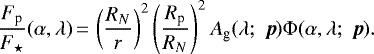
Our atmospheric model is sketched in Fig. 1 and described by the six parameters in the atmospheric vector p = {τc, Δc, τc →TOA, reff, ω0,  }. Here, τc is the optical thickness of the cloud and Δc its geometrical vertical extension. The cloud layer is assumed to be horizontally homogeneous over the whole planet. The optical thickness of gas from the cloud top to the top of the atmosphere (TOA) at the reference wavelength λ* is given by τc →TOA. This is a measure of the altitude or pressure level at which the cloud top is located. ω0 is the single scattering albedo of the cloud aerosols, which we leave as a free parameter to account for different aerosol compositions. Both τc and ω0 are assumed to be wavelength independent. In our treatment, the effective radius of the aerosols (reff) defines their scattering phase functions. We have calculated the scattering phase function p(θ) for each reff through Mie theory assuming a constant refractive index of 1.42 specific to NH3. Our treatment preserves the expected trend that small effective radii reff will result in nearly isotropic scattering phase functions, whereas large values will result in enhanced backward and forward scattering. The scattering phase functions are shown in Fig. 2. By varying ω0 and reff independently, our exploration is generalized to clouds with arbitrary composition. Lastly,
  stands for the relative methane abundance or volume mixing ratio relative to H2 -He, assumed constant over all layers. The CH4 opacities are taken from Karkoschka (1994).
Each of the six parameters is given the set of values summarized in Table 1 to obtain a dense grid of atmospheric configurations (~300 000 configurations after omitting impossible situations in which the cloud’s vertical extension reaches below the model’s deepest layer). For each of these configurations we obtain a synthetic spectrum, as described below. This dense grid of spectra is used during the retrieval process to obtain new spectra from interpolation within the grid at p configurations not represented in Table 1 (see Sect. 3.3).
We discretize the atmosphere with a total of Nslabs = 28 vertical slabs, each of them of geometrical thickness Hg/2. The scattering and absorption coefficients are assumed to be constant within each slab, and we follow standard rules when averaging over the gas and aerosols. The optical thickness of gas above each interface k (see Fig. 1) is τk = τk = 0 exp(−k∕2). Clouds are placed over an integer number of scale heights (Δc /Hg = 1, 2, 3,..., 8). Once the atmospheric model is set up and p prescribed, we produce the reflected-starlight spectra by solving the radiative transfer equation for multiple scattering with a backward Monte Carlo (BMC) model (García Muñoz & Mills 2015). The BMC model has been thoroughly tested against phase curve calculations (Dlugach & Yanovitskij 1974; Buenzli & Schmid 2009) with excellent agreement, and against whole-disc polarization and brightness phase curves of Venus and Titan (García Muñoz et al. 2014, 2017; García Muñoz & Mills 2015; García Muñoz & Isaak 2015; Ilic et al. 2018). Two reasons for using the BMC model instead of other, probably faster, radiative transfer solvers are to secure the accuracy of eventual calculations at all possible phase angles, and to be able to extend the analysis to polarization in the future.
Our description of atmospheric stratification relies on optical thickness, rather than altitude or pressure. Although the actual implementation into the BMC model uses altitude and therefore a scale height, the value of Hg disappears from the description of τk (see above) and in turn from the description of the atmosphere. In other words, the value of Hg is irrelevant for small and moderate phase angles, and our implementation is essentially independent of this parameter. This may not be true at large phase angles (García Muñoz et al. 2017; García Muñoz & Cabrera 2018), but this scenario is impractical in direct imaging due to the visibility restrictions imposed by the technique. As a check, in a few hundred cases we solved the radiative transfer equation for different Hg values while keeping the rest of the parameters unaltered. No differences were observed in the generated spectra, thereby confirming that Hg plays no role in our simulations.
For each combination of the parameters in the atmospheric vector p we computed synthetic spectra in the range 500−900 nm. Figure 3 shows (solid black lines) the spectrum of a particular atmospheric configuration referred to as thin-cloud (see Table 2). Also plotted are the spectra corresponding to varying the elements of p one at a time through the grid of simulations of Table 1. We used a spectral bin Δλ = 4 nm over theentire spectral range, which was deemed appropriate because the absorption features by CH4 are broad. This translates into resolving powers of R ~ 125 at 500 nm and R ~ 225 at 900 nm.
Our approach does not include photochemistry or the microphysics of cloud formation. Instead, we parameterize the optical properties of the gas and aerosols and explore the influence of a few key properties on the synthetic spectra. This is complementary to other approaches (e.g. Ackerman & Marley 2001; Ohno & Okuzumi 2017; Helling et al. 2017; Damiano & Hu 2019) that investigate the photochemical and microphysical mechanisms resulting in cloud formation. Scanning through all six parameters in our atmospheric model gives us a broad view of possibilities that can eventually be tested against more physically based approaches.
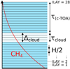 |
Fig. 1 Sketch of the vertical structure in our atmospheric model. ILAY denotes each of the slabs into which the atmosphere is divided, each with thickness Hg ∕2. Gas density decreases exponentially with height. The atmosphere is assumed to contain CH4, with a certain fraction |

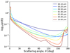 |
Fig. 2 Scattering phase functions for the considered values of reff. |
Values for the parameters in the atmospheric vector p used to construct the grid of synthetic reflected-starlight spectra.
 |
Fig. 3 Solid black lines: synthetic spectra for the thin-cloud configuration (see Table 2). Coloured lines: synthetic spectra for the configurations that result from perturbing each of the elements of the six-dimensional atmospheric vector p = {τc, Δc, τc →TOA, reff, ω0,
|

Adopted true values for the model parameters.
3 Retrieval procedure
Observing exoplanets in direct imaging will allow us to estimate the planet radius and atmospheric composition from retrieval exercises of the measured spectra. One of the aims of this work is to quantify the uncertainties in the estimates of the retrieved properties. Since there are no measurements of this kind yet, we conduct the exercise through simulated measurements. From these, we attempt to extract information through the systematic comparison with synthetic spectra.
3.1 Adopted true configurations
We adopt three of the atmospheric configurations in our grid of Table 1 as true, meaning that they represent the true atmosphericproperties of the planet that is being observed. These configurations are identical in all the parameter values except τc, so we can specifically explore the transition from cloud-free to thick-cloud conditions. We will refer to the three atmosphericconfigurations as the no-, thin-, and thick-cloud scenarios. They are summarized in Table 2.
We include the planet radius as an optional free parameter. All these (6 + 1) properties will be unknown to the observer, with the possible exception of the radius if the planet happens to transit. In the particular case of Barnard b, none of these properties is known for the time being. Hence, the true atmospheric configurations are hypothetical, although physically reasonable as described below. The probability of transit for a randomly oriented orbit is ~ R⋆/r, where R⋆ is the stellar radius (Borucki & Summers 1984). This amounts to 0.2% (R⋆ = 0.178 R⊙) for Barnard b. The transit probability is small but not negligible, and thus it is important to consider both situations in which the planet radius is either known or unknown.
The true parameter values of Table 2 are motivated by atmospheric models of the solar system gas planets. For instance, τc = 1.0 is comparable to the optical thickness of 0.5 used by Schmid et al. (2011) to model a set of spectropolarimetric measurements of Jupiter at wavelengths 520–935 nm. For our no-cloud and thick-cloud configurations, we use τc = 0.05 and τc = 20 respectively. These stand for lower and upper extremes of the values that τc may take, in order to explore the influence of cloud prevalence on exoplanet characterization.
Following Smith & Tomasko (1984), Schmid et al. (2011) also considered that the cloud is overlaid by a gas layer of optical thickness τgas = 0.011, which is consistent with the τc→TOA = 9.1 × 10⁻³ used here. A cloud with a geometric extension Δc = 2Hg is rather narrow, a property also expected for the upper clouds of the solar system gas giants (Sánchez-Lavega et al. 2004). Our reff = 0.5 μm choice for the effective radius of the aerosols corresponds to moderately small particles. Mishchenko (1989) examined ground-based spectropolarimetric observations of Jupiter at wavelengths of 423–798 nm. Their best-fit model consisted of tropospheric aerosols of reff = 0.39 ± 0.08μm, in the order of our assumed reff. Sizes of reff = 0.4 μm were also reported by Morozhenko & Yanovitskij (1973) for polarization measurements of Jupiter between 373–800 nm, and Pérez-Hoyos et al. (2012) modelled the tropospheric aerosols of Jupiter with reff = 0.75 μm. Our single-scattering albedo ω0 = 0.90 is slightly low compared for example to Schmid et al. (2011), but within the ranges usually considered in the literature (e.g. Satoh et al. 2000; Pérez-Hoyos et al. 2012). The methane abundance that we adopt ( = 5 × 10⁻³) is comparable to that of Jupiter (2.1 × 10⁻³) and Saturn (4.5 × 10⁻³) but somewhat lower than for Uranus or Neptune (2.4 × 10⁻² and 3.5 × 10⁻², respectively) (Sánchez-Lavega 2010).
Our choice for the planetary radius, Rp∕RN = 0.6, corresponds to a density of Barnard b equal to that of Neptune and the mass for an edge-on orbit (Mp = Mmin∕sin(90°)). According to Barros et al. (2017), this mass and radius would correspond to a gaseous exoplanet. Any other orbital inclination would suggest a more massive and probably larger planet size, entailing better conditions for the planet to retain a H2 –He atmosphere. This would also yield more favourable planet-to-star contrast ratios at a given phase angle. Our choice is therefore somewhat conservative in terms of planet-to-star contrasts.
3.2 Noise model
We produce the measured spectra by adding noise to the true spectra. Our noise model is described by a single parameter, namely the S/N. The added noise is given by a normal distribution of zero mean and standard deviation,
 (2)
(2)
where  is the maximum contrast over the filter band for the true spectrum, which typically occurs in the continuum near 500 nm. As defined here, σm is wavelength independent and budgets in a variety of noise sources that are not explicitly considered such as dark current, speckle noise, and leakage of stray starlight (Marois et al. 2000; Wahhaj et al. 2015; Robinson et al. 2016). The parameter S/N can be viewed as the maximum S/N over the whole measured spectrum. In our retrievals, we adopt S∕N = 10. Figure 4 shows both the true (synthetic, without noise) and measured (after adding noise) spectra for the three cloud scenarios considered.
Admittedly, our approach to the noise model does not account for all the complexity in the noise of a real observation from a particular telescope. Future work will update our noise model to a more realistic one that considers that the S/N of a real observation may deteriorate more in the stronger absorption bands, and that the sensitivity of a real instrument varies with wavelength. We also note that the angular separation between planet and star will affect the S/N, as positions closer to the inner working angle (IWA) of the instrument will result in noisier observations (Lacy et al. 2019). Although the final specifications of future space-based coronagraphs are not yet defined, works such as Robinson et al. (2016) or Lacy et al. (2019) have started to consider instrument-specific noise models and their implications.
Further, we note that a simplified noise model allows us to focus on the difficulties in the interpretation of reflected-starlight spectra, which are fundamental to the radiative transfer problem, sidestepping instrument-specific difficulties. In this respect, we describe in Sect. 4.1 that our retrievals for a known planetary radius Rp show behaviours similar to those reported in previous works that used more complex noise models. This consistency check confirms that our findings are not critically affected by the adopted noise model. In other words, our simplified noise model (see Sect. 4.2) serves to set theoretical limits to how much information can be retrieved from a measured spectrum.
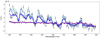 |
Fig. 4 Solid lines: true (noiseless) spectra for the three atmospheric configurations in Table 2 at phase angle α = 0°. Symbols: corresponding measured spectra, with error bars specific to S∕N = 10. The size of the error bars (σm; see text) is defined on the basis of the brightest spectral bin (which typically occurs near 500 nm) and is the same at all wavelengths for each spectrum. The spectra correspond to no-cloud (light blue), thin-cloud (dark blue), and thick-cloud (purple) atmospheric configurations. |
3.3 Exploring the parameter space
Once the measured spectrum is simulated for each of the true configurations (Table 2), we address the retrieval. We assess whether from such an observation we are able to correctly infer the properties of the exoplanet. This requires a thorough exploration of the parameter space, testing multiple combinations of the parameter vector p, and checking whether they produce spectra similar to the measured one. The vector p includes the atmospheric model parameters (see Table 1) and, when the planet radius is assumed to be unconstrained, also Rp ∕RN.
To have a continuous representation of the parameter space, we opt to sample p continuously. For that, we use the Markov chain Monte Carlo (MCMC) sampler emcee (Foreman-Mackey et al. 2013). This MCMC sampler proposes test points (ptest) in the multi-dimensional parameter space p and evaluates the likelihood of such a test configuration to have produced the measured spectrum. It does so by comparing the synthetic spectrum corresponding to that ptest with the measured spectrum. Test spectra are generated through linear interpolation within the pre-computed grid of synthetic spectra (Table 1). This approach is much faster than solving the multiple-scattering radiative transfer equation at each test configuration ptest sampled by emcee. In Appendix A we prove the accuracy of producing the test spectra through interpolation from the grid, compared to computing each of them by solving the radiative transfer equation. Figure A.1 shows that we produce virtually the same spectra in both cases.
When comparing a test spectrum to the measured one, we quantify how similar they are through the figure of merit,
 (3)
(3)
where Fp∕F⋆ is the planet-to-star contrast ratio (Eq. (1)) and σm is the standard deviation for the noise (Eq. (2)) (Bevington & Robinson 2003).
Although the sampler tests the whole space of parameters, at the time of proposing a new point to test, those regions of p with lower values of χ2 will be favoured. Hence, it will tend to test more frequently such regions since they are considered more likely to have produced the measured spectrum and therefore more interesting to study. This sampling process is carried out simultaneously by several chains (or walkers) so that the space of the parameters is sampled multiple times independently, to avoid falling into local minima of χ2.
The limits of the parameter space exploration are set by the box priors described in Table 3. We note that in retrieval cases where the radius of the exoplanet is known, Rp is not explored and thus the sampler moves in a 6D parameter space. On the other hand, if Rp is considered unknown, the sampler searches in a 7D parameter space. As shown in Table 3, some parameters (τc, τc →TOA,  , Rp ∕RN) are sampled by emcee in logarithmic scale. We verified that this ensures an optimal performance both during sampling and interpolation.
The MCMC sampling is performed using a total of 500 walkers. The ensemble of walkers runs for a maximum of 105 steps, producing a total set of 5 × 10⁷ samples. We apply a convergence criterion to stop the run if the number of iterations surpasses 50 times the autocorrelation time. The autocorrelation time provides a measure of the sampler performance and whether it is obtaining independent samples from the space of parameters (Goodman & Weare 2010). With this convergence criterion, we make sure that the sampling is sufficiently complete, regardless of local minima (Foreman-Mackey et al. 2013). A burn-in phase is considered, discarding the samples from the first n iterations, where n corresponds to the autocorrelation time.
Other related works have approached the retrieval by sampling the parameter space from a uniform grid instead of randomly choosing the sampling points (e.g. Madhusudhan & Seager 2009; von Paris et al. 2013; García Muñoz & Isaak 2015). On the other hand, in for example Lupu et al. (2016), Nayak et al. (2017), and Damiano & Hu (2019) the sampling points are selected by MCMC or multi-modal nesting methods and the synthetic spectrum generated by solving the radiative transfer equation for that particular configuration. Compared to interpolating, solving the multiple-scattering problem at each test point ptest of the sampling results in a much slower performance of the retrieval process. Hence, our approach combines a MCMC sampling with the efficiency of interpolating from a pre-computed grid of synthetic spectra.
Priors used for each of the model parameters.
4 Results
We will explore here the retrieval results for the three atmospheric scenarios described in Table 2. As an initial exercise, we assume that the planet radius Rp is known. In this case, the MCMC sampler is run as described in Sect. 3 with the six free parameters of the atmospheric model. Afterwards, we repeat the retrieval analysis but considering that the planet radius is unconstrained. In the latter case, Rp ∕RN will be considered a free parameter and therefore the MCMC sampler will explore a 7D parameter space. We finally discuss how the retrieval results change when the planetary radius is known to within some degree of uncertainty.
4.1 Retrieval if Rp is known
For a S∕N = 10, we simulated the measured spectra for the no-cloud, thin-cloud, and thick-cloud configurations (Table 2) and ran the MCMC sampler. After discarding the initial burn-in samples, we were left with approximately six million samples in each exploration. Each sample corresponds to a particular atmospheric configuration with its corresponding synthetic spectrum and χ2.
We confirmed that many different atmospheric configurations produce spectra that are nearly identical to the measured one. Figure 5 shows all the spectra that meet the condition  for each of the cloud scenarios. For Gaussian distributions, the set of spectra meeting this criterion contains the best-fitting configuration with a 99.99% probability (Press et al. 2007). Figure 5 also shows the true and measured spectra for observations at S∕N = 10 with a known valueof Rp. Figures 6 and B.1–B.2 show the retrieval results for the three cloud scenarios and, together with Fig. 5, give a sense of the parameter correlations and their effects on the spectra. The two-dimensional posterior probability distributions in Figs. 6 and B.1–B.2 identify correlations between each pair of model parameters. Contour lines indicate the 0.5, 1, 1.5, and 2σ levels that bracket the 12, 39, 68, and 86% confidence intervals, respectively. The marginalized one-dimensional probability distributions depict the computed likelihood of finding the solution for each parameter in a certain range of values. For comparison, the green points and lines in the figures mark the true parameter values. Table 4 summarizes the retrieval results. The quoted values correspond to the median of the marginalized probability distributions. Upper and lower limits define the intervals within the 84 and 16% quantiles, respectively. This corresponds to the 68% confidence interval. The meaning of the confidence intervals is lost in cases where only upper or lower limits can be set on the model parameters, as described below.
In all cases, for observations at S∕N = 10, the retrievals can discriminate reasonably well between cloudy and cloud-free atmospheres. However, the retrievals do a poorer job at estimating the optical thickness of the cloud, regardless of the true τc. In the no-cloud case (Fig. 6), the probability distribution of log (τc) peaks towards negative values, with an estimated log (τc) =  . Even if the retrieval overestimates the true log (τc) = − 1.30, it shows strong evidence of an atmosphere with no cloud or with an extremely thin one. Indeed, the probability distribution indicates that the values ofτc quoted from the retrieval must be interpreted as upper limits, and that the quoted uncertainties lose their usual meaning. In the thin-cloud scenario (Fig. B.1) the estimated log (τc) =
  is lower than the true one, log (τc) = 0.0. However, the marginalized probability distribution of log (τc) suggests thepresence of a thin cloud, and tends to rule out both the no-cloud and thick-cloud configurations. Finally, the thick-cloud configuration (Fig. B.2) produces a probability distribution for log (τc) that rules out any cloud-free atmospheric configuration. This sets a sharp lower limit for τc, meaning that in this case the detection of a cloud is evident, although its optical thickness remains poorly constrained.
We find that the retrieved  differs morefrom the true abundances as the optical thickness of the cloud increases. We interpret this as a consequence of scattering and absorption within the cloud that interferes with CH4 absorption, thereby modifying the band-to-continuum contrast in the spectra. Indeed, the 2D probability distributions show a complex coupling of
  with cloud properties, primarily log (τc) and τc →TOA. In our retrievals, the estimates for both τc and τc→TOA tend to deviate from the true values, affecting the retrieved value of
  . Consistently, our best-fitting estimate for log (
 ) is obtained for the no-cloud scenario (see Table 4).
The location of the cloud top τc→TOA is poorly constrained in the no-cloud and thin-cloud cases. This is not surprising as the impact of a cloud on the spectral appearance in these cases is weak or moderate. In the thick-cloud scenario (see Fig. B.2), the marginalized probability of τc →TOA tends to rule out configurations in which the cloud is located either very deep or very high. The effects of having such an optically thick cloud at those positions would be apparent in the spectrum. For instance, a deep cloud is concealed by the gas in the upper atmospheric layers. Hence, the resulting spectrum would be effectively equivalent to that of a thin-cloud or even a cloud-free configuration. As discussed above, the retrieval at S∕N = 10 tends to discard such scenarios for the thick-cloud configuration. In turn, a high-altitude cloud entails that CH4 absorption diminishes to levels inconsistent with the measured spectrum, a situation that is also easily identified. Regarding the geometrical extension of the cloud Δc, it is virtually unconstrained in all cases for this S/N.
The single-scattering albedo of the aerosols ω0 is systematically underestimated in the retrievals, especially for the thick-cloud case. This has implications on prospective efforts to identify the nature of the cloud particles through their refractive index. Furthermore, the inferred ω0 shows strong correlations with both τc and reff. The ω0 –reff correlation is explained by the fact that ω0 and the scattering phase function p(θ) multiply each other in the radiative transfer equation. Indeed, within the limit of single scattering, the amount of scattered light is proportional to ω0 ⋅ p(θ). The fact that p(θ) is dependent on reff explains the two branches observed in the 2D probability distribution for ω0 –reff (see Fig. B.2). Figure 2 shows that for θ = 180° (backward scattering, dominating at α = 0°), p(θ) presents a minimum around reff = 0.50 μm. Thus, in this viewing geometry, a similar amount of photons would be reflected for any other reff (which means that p(θ = 180°) increases) if ω0 is reduced. This creates numerous possibilities to reproduce the measured spectrum with ω0 values smaller than the true one. This degeneracy depends on the shape of the scattering phase function of the aerosols, whose value changes with the viewing geometry. In future work we will explore the prospects for breaking this degeneracy with observationsat multiple phases.
The ω0 –τc correlation reveals the impact that cloud absorption has on the spectrum. In the thick-cloud scenario, such a thick cloud (estimated log(τc) =  ), with aerosols of estimated ω0 =
  , absorbs a certain amount of incoming photons. This absorption shapes the reflected-light spectrum, especially in the continuum. However, a similar spectral shape may result from an optically thinner cloud composed of darker aerosols (see Fig. B.2). In other words, both parameters can compensate each other and yield a similar amount of continuum absorption. The same idea applies to the thin-cloud case (Fig. B.1), although the correlation there is not so strong due to the smaller optical thickness.
Our retrieval results for a known value of Rp are consistent with previous literature. Although the model setups differ between the different studies, we observe that, for those parameters that are comparable, our results behave similarly. For instance, analogous correlations between gaseous-species absorption and cloud pressure level were discussed for example by Heidinger & Stephens (2000), Lupu et al. (2016), and Damiano & Hu (2019). Correlations between cloud properties (scattering and absorption properties; optical thickness and pressure level) were also observed for example in Heidinger & Stephens (2000) and Lupu et al. (2016). As the noise models in all those cases differ, these similarities drive us to conclude, on the one hand, that our noise model approach does not blur the physical fundamentals of the exercise. On the other hand, this ensures that our results for a known Rp are well founded in order to move on and compare them to the case of an unknown Rp.
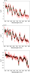 |
Fig. 5 Solid green line: true spectrum for the true atmospheric configuration. Red symbols: simulated measured spectrum, with error bars corresponding to S∕N = 10. Solid black lines: synthetic spectra that meet the condition Δχ2 < 15.1, generated during the MCMC retrieval for a known Rp. Top: no-cloud configuration; middle: thin-cloud; bottom: thick-cloud. |
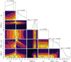 |
Fig. 6 Posterior probability distributions of the model parameters for a simulated observation of the no-cloud atmospheric configuration at S∕N = 10. The planetary radius is assumed to be known and Rp∕RN = 0.6. Green lines mark the true values of the model parameters (see Table 2) for this observation. Two-dimensional subplots show the correlations between pairs of parameters. Contour lines correspond to the 0.5, 1, 1.5, and 2σ levels. The median of each parameter’s distribution is shown on top of their 1D probability histogram. Upper and lower uncertainties correspond to the 84 and 16% quantiles. The figures corresponding to the other scenarios discussed in Sects. 4.1 and 4.2 are shown in Appendix B. |
Retrieval results for the case of known Rp.
Retrieval results for the case of unknown Rp.
4.2 Retrieval if Rp is unknown
We repeated the previous study but now including the planetary radius Rp ∕RN as an additional free parameter to be explored with the MCMC sampler. The priors for this parameter (see Table 3) mean that the value of Rp is completely unconstrained. Again, in this exercise, we adopt a S∕N = 10. The corresponding retrieval results are summarized in Table 5. We display in Fig. 7 the spectra meeting the Δχ2 < 15.1 criterion for the three cloud cases. The posterior probability distributions are shown in Figs. B.3–B.5 for the no-cloud, thin-cloud, and thick-cloud scenarios, respectively.
Interestingly, it is feasible to constrain reasonably well the planet radius for all cloud scenarios. The estimates of Rp ∕RN for the no-cloud (Fig. B.3) and thin-cloud configurations (Fig. B.4) are in agreement with the true value Rp ∕RN = 0.6, even at a S∕N = 10 (see Table 5). The upper and lower boundaries of these estimates allow us to constrain Rp ∕RN to within less than a factor of two from the true value. Namely, for the no-cloud atmosphere the confidence interval of Rp ∕RN ranges between 0.51 and 0.83. This compares well with the true Rp∕RN = 0.6. In the thin-cloud case, Rp∕RN is constrained between 0.44 and 0.74. However, if the atmosphere contains a thick cloud (Fig. B.5), the retrieved Rp ∕RN is significantly less accurate. Here, the median of the probability distribution (log (Rp∕RN) = − 0.41) deviates more from the true value (log (Rp∕RN) = − 0.22 than in the other cloud scenarios. Still, in this thick-cloud case the planet radius is constrained to within a factor of approximately two (ranging from Rp∕RN = 0.29 to 0.66).
Our finding that it is possible to constrain Rp to within a factor of two is consistent with the results of Nayak et al. (2017), who studied the correlations between phase angle α and Rp, with both parameters unknown a priori. Their study, however, did not focus on analysing which new correlations between atmospheric parameters are generated by including Rp as a free parameter. By comparing fixed-Rp and free-Rp retrievals, we show that there are indeed important degeneracies involved between Rp and atmospheric parameters such as τc. Here we prove that constraining Rp to within a factor of two is a result that is valid regardless of the presence or absence of clouds or their optical thickness. As the cloud coverage of an exoplanet will not be known beforehand, this sets an encouraging perspective to estimate the radius of non-transiting exoplanets.
Detecting the presence or absence of clouds is not evident in any case if the planet radius is unknown. For a no-cloud atmosphere, the estimated log (τc) value is  (Table 5), larger than the result obtained for a known Rp (
 , see Table 4). We note in the upper error of these results that the confidence interval in the case of an unknown Rp reaches higher values of τc. Graphically, this is shown in the 1D probability distribution of log (τc) from Fig. B.3, in comparison with that in Fig. 6 for a known Rp. The log (τc) probability distribution for the thin-cloud scenario is also broader if Rp is unknown. Indeed, the marginalized probability distribution (see Fig. B.4) shows in this case the same likelihood for a cloud with optical thickness log (τc) = 0.0 (the true value) and for a log (τc) = − 1.2 (that effectively corresponds to a cloud-free atmosphere). In both Figs. B.4and B.5 we observe practically equivalent upper limits for the value of τc. Thus, the no-cloud and thin-cloud scenarios would become indistinguishable if Rp is unknown.
The change in the log(τc) probability distribution with respect to the case of known Rp is more dramatic in the thick-cloud retrieval (Fig. B.5). Here, the 1D probability distribution becomes almost flat and its median presents wide upper and lower errors (log(τc) =  ). Hence, the posterior distribution reveals comparable probabilities of having observed a planet with thick cloudsor with a cloud-free atmosphere. This is in great contrast with the retrieval for a known Rp, in which case the thick-cloud retrieval shows an unambiguous cloud detection (Fig. B.2).
The methane abundance is also worse constrained when Rp is unknown, with larger ranges of possible values consistent with the measured spectrum (Table 5). As was the case for known Rp, the thick-cloud scenario shows the poorest  estimates (Fig. B.5). In this case,
  is strongly underestimated, demonstrating again the physical degeneracy between
  and τc, which is also underestimated in this thick-cloud retrieval.
This degeneracy also affects the no-cloud and thin-cloud retrievals (Figs. B.3and B.4). We note that in both cases the 1D posterior probability distributions of τc are very similar. This is a consequence of the Rp uncertainties, which have a great effect on the spectrum. Compared to such a strong influence of Rp ∕RN, the impact on the spectrum of having a cloud with τc = 0.05 or τc = 1.0 becomes negligible. This makes it challenging to distinguish between a no-cloud and a thin-cloud atmosphere. Nevertheless, the deviation of these 1D posterior distributions with respect to the true values is much larger in the no-cloud scenario. Overestimating τc, therefore, produces an increase in the resulting estimate of  . That is the reason why, if Rp is unconstrained, the no-cloud atmospheric configurations do not necessarily yield the best estimates of
  .
.
The restof properties of the cloud (τc→TOA, Δc) and its aerosols (reff, ω0) are generally unconstrained in all three scenarios. Figure 3 shows, for the thin-cloud atmosphere, the effects that modifying each of the atmospheric model parameters produces on the reflected-light spectrum. Figure 8 repeats this exercise for Rp ∕RN. From the comparison of both figures, we observe that Fp /F⋆ undergoes larger variations when Rp∕RN is modified than when the other parameters are modified. This suggests that introducing Rp ∕RN as a free parameter makes this parameter a dominating source of uncertainty in the retrieval.
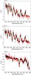 |
Fig. 7 As Fig. 5, but for retrievals where the planetary radius is unknown. Top: no-cloud configuration; middle: thin-cloud; bottom: thick-cloud. |
4.3 Intermediate uncertainties in Rp
So far we have considered two limiting cases for our retrievals: one with a known, fixed value of the planet radius, the other one, with Rp∕RN as a free parameter. This exercise allowed us to understand the influence of Rp on the retrievaloutcome. However, it is possible that we will encounter exoplanets whose radius is not completely unconstrained, but rather known to some extent.
For instance, this would be the case for exoplanets discovered in radial-velocity surveys. In combination with other techniques such as astrometry, the planet mass could be estimated. With that, mass-radius relationships would yield a range of values for Rp. We note the inherent inaccuracy of such mass-radius relationships, as the planet composition and density will not be known a priori. The suitability of these relations needs to be discussed for each specific planet. However, even with these caveats, mass-radius relationships will offer at the very least a range of possibilities for the planet density and, hence, a hypothetical range of possible Rp values. Furthermore, uncertainties in the estimates of Rp from transit observations might reach values close to 10% depending on the planet size and the stellar parameters (Rauer et al. 2014). In these cases, Rp would not be completely unconstrained. This motivates us to study how different radius uncertainties would impact the characterization of the exoplanet via direct imaging.
In this setting, we explored how the outcomes of the retrieval are affected by different levels of uncertainty in the a priori estimates of Rp∕RN (ΔRp). Table 6 shows the retrieval results for the three cloud scenarios and ΔRp = 0, 1.6, 10, 25, and 50%, as well as for an unconstrained value of Rp. Here, the box priors for Rp∕RN in the MCMC retrieval sampler correspond to each ΔRp, while the rest of the parameters had the same box priors as in Table 3. As above, we set S/N = 10.
Figure 9 shows that reducing ΔRp tends to provide better estimates of τc and  . The conclusions on the other model parameters do not change appreciably with respect to the retrievals for both Rp ∕RN known or unknown. We argue that reducing ΔRp partially breaks some of the correlations between parameters, which are boosted if Rp ∕RN is set as a free parameter. Namely, reducing the Rp –τc degeneracy affects other parameter correlations, thus improving the estimates of
  . In accordance with this, the improvement in the retrievals as the uncertainty in Rp ∕RN decreases is more evident in the thick-cloud scenario. Given the large optical thickness of the cloud in this scenario, the Rp -τc correlation had a bigger impact on the retrievals than for no-cloud or thin-cloud cases.
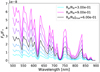 |
Fig. 8 Black line: synthetic spectrum for the thin-cloud configuration (Table 2). Colour lines: synthetic spectra for the configurations that result from perturbing Rp ∕RN. The colour code is described in the legend for the lowermost and uppermost values. Intermediate colours span over the values Rp∕RN = {0.40, 0.50, 0.60, 0.70, 0.80}. This corresponds to a radius uncertainty of ΔRp = 33%. |
4.4 Impact of noise realizations
In Sects. 4.1 and 4.2, we have presented retrieval results based on the measured spectra of Fig. 4, and therefore on single noise realizations. To confirm that these conclusions do not strongly depend on the randomly generated noise, we repeated each of the retrievals nine more times for different noise realizations at S∕N = 10. Figure C.1 summarizes the outcome of this exercise, confirming that the findings reported above are generally robust.
Retrieval results for different levels of uncertainty in the value of Rp∕RN.
5 Conclusions
Scheduled to be launched in 2025, WFIRST will be the first direct imaging space mission to obtain spectra of reflected starlight from cold exoplanets and it will open a new field of research into exoplanetary atmospheres. Due to constraints in contrast and angular separation, WFIRST will mostly observe long-period giant planets. However, for special cases it might also reach the interesting range of super-Earth to mini-Neptune exoplanets, not existent in the solar system. Many of those targets are expected to have H2 –He atmospheresand clouds with a diverse range of optical properties. Understanding how each atmospheric parameter affects the reflected-light spectra of those planets will pave the way for future direct imaging missions such as LUVOIR or HabEx. These will be focused on characterizing the atmospheres of Earth-like planets.
In this work we have explored what properties of an atmosphere would be possible to infer from a direct-imaging spectroscopic measurement. For that, we have created an atmospheric model with six free parameters that was outlined in Sect. 2. This description is consistent with the structure of gas- and ice-giants in the solar system. Then, using a previously validated radiative transfer code, we computed the synthetic spectra for ~300 000 atmospheric configurations at phase angle α = 0°. We analysed how different atmospheric configurations may generate similar spectra with a set of retrieval exercises. In each retrieval, wesimulated a measured spectrum by adding noise at a certain S/N to the spectrum computed for an assumed true atmosphericconfiguration. Afterwards, we used a MCMC sampler to explore the space of parameters in search of atmospheric configurations yielding a spectrum consistent with the measured one. We also tested the influence of including the planet radius as a free parameter in the retrieval, and thus sampling a 7D space instead of a 6D one. This is a relevant question since most of the long-period exoplanets that will be observable with direct-imaging techniques will not transit and thus their radius will remain uncertain.
We specified this analysis to the planet candidate Barnard b (Ribas et al. 2018). This is a realistic case as the proximity of its host star and its orbital parameters make it a very promising candidate for direct-imaging observations. Indeed, we showed that both the angular separation and contrast of this exoplanet are in the operating range of WFIRST (Spergel et al. 2015; Trauger et al. 2016). Therefore, this mission would be able to detect Barnard b in direct imaging and start characterizing its atmosphere. Eventual spectra taken by WFIRST will not have the full wavelength coverage between 500 and 900 nm or the resolving power used here. Lacy et al. (2019) reported that the filters that will finally fly with the telescope are still to be decided, with only one filter guaranteed for spectroscopy so far. We will quantify in future work the exact influence of partial spectral coverage on the atmospheric characterization. However, a wide spectral coverage will surely improve the potential of WFIRST and the next-generation direct-imaging missions to analyse exoplanetary atmospheres.
The retrieval exercise was run for three different true atmospheric configurations: one with virtually no clouds (τc = 0.05), another with a thin cloud layer (τc = 1.0), and finally one with an optically thick cloud (τc = 20.0). If the value of Rp is known, we found that observations at S∕N = 10 yielded evidence of the presence or absence of clouds in each of the cloud scenarios. The optical thickness of the cloud, however, was not accurately constrained in any of the three cases. The retrievals also detected the presence of methane in the atmosphere. Furthermore, it was possible to constrain the CH4 abundance with reasonable success in the three cloud scenarios. The rest of the model parameters, on the other hand, remain largely unconstrained. We identified a correlation amongst the optical properties of the cloud aerosols that prevents a reliable estimate of the aerosols’ single scattering albedo, which is potentially informative of their composition.
The main result of our study is that an unknown planetary radius will prevent the detection of the presence or absence of clouds. Uncertainties in Rp trigger physical degeneracies between model parameters, particularly between Rp, the optical depth of the cloud (τc), its pressure level (here given by τc→TOA), and the CH4 abundance ( ). These correlations blur the atmospheric information that is possible to extract when Rp is known. Hence, we conclude that predictions for atmospheric characterization built upon retrieval exercises in which Rp is assumed to be known are overly optimistic. They should be taken as ideal, best-case scenarios.
We also find that, if the radius of the exoplanet is completely unknown a priori, an observation with S∕N = 10 could constrain it to within a factor of approximately two. This estimate is consistent with the findings by Nayak et al. (2017), who focus on the Rp -α correlation. We here showed that this result holds true regardless of the cloud coverage of the exoplanet. This is a non-trivial finding, as we also show that Rp is highly correlated with the optical thickness of the clouds in the atmosphere. Indeed, if the cloud is very thick, we found that the most likely estimates of Rp deviate more from the true value, although still within a factor of approximately two. How the τc –Rp degeneracy unfolds for several S/N levels will be a matter of future work.
Furthermore, we show that reducing the uncertainties in the a priori estimate of Rp results in more accurate retrievals of τc and  . With this, we outline how direct-imaging studies could benefit from other observational techniques as well as theoretical works on mass-radius relationships.
Nevertheless, constraining the radius of non-transiting exoplanets to a factor of two will potentially narrow the set of compatible internal compositions. Achieving this independently of a priori unknowns, such as the atmospheric cloud coverage, would help in the understanding of the diversity and size distribution of the exoplanet population. Currently, the population of exoplanets suitable for these direct-imaging measurements remains modest. However, this population is expected to grow steadily as different techniques (radial velocity, astrometry, transit photometry) continue surveying the sky. It is essential to exploit the synergies between different techniques to maximize the possibilities to characterize the atmospheres of long-period exoplanets.
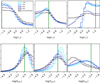 |
Fig. 9 Marginalized probability distributions for τc
(top) and |

Acknowledgements
The authors acknowledge the support of the DFG priority program SPP 1992 “Exploring the Diversity of Extrasolar Planets (GA 2557/1-1)”. N.C.S. acknowledges the support by FCT - Fundação para a Ciência e a Tecnologia through national funds and by FEDER through COMPETE2020 - Programa Operacional Competitividade e Internacionalização by these grants: UID/FIS/04434/2019; UIDB/04434/2020; UIDP/04434/2020; PTDC/FIS-AST/32113/2017 & POCI-01-0145-FEDER-032113; PTDC/FIS-AST/28953/2017 & POCI-01-0145-FEDER-028953.
Appendix A Completeness and interpolation of the grid of spectra
Our approach to the inversion problem relies on sampling continuously the six-dimensional atmospheric vector p = {τc, Δc, τc →TOA, reff, ω0,  } from the discreet grid summarized in Table 1. To that end, we must ensure that the grid is dense enough, and devise a way to predict the spectra for atmospheric configurations not represented in the grid.
The differences between consecutive spectra are small for the specific example shown in Fig. 3. They are also small in general, which simply confirms that our grid is dense. To sample continuously in p, we opted to interpolate linearly within the multiple dimensions of the grid of spectra with the scipy interpolate routine (Virtanen et al. 2020).To test the accuracy of this approach, we compared the albedos interpolated at 1000 random realizations of p against the exact solutions obtained by solving the scattering problem with the backward Monte Carlo model. These 1000 random realizations of p were generated by sampling each variable from a uniform distribution between the limits set in Table 3. We define the figure ofmerit for the comparison as
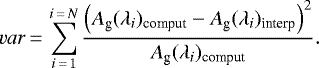 (A.1)
(A.1)
Figure A.1 shows the histograms for the var values from the comparison. The albedo corresponding to the highest var (and poorest performance of the linear interpolator) is shown in Fig. A.1. The exercise confirms that our adopted interpolation is an accurate way of producing spectra at arbitrary p realizations provided that the grid of spectra is dense enough, as is the case here.
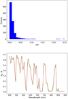 |
Fig. A.1 Top: distribution of var values for the 1000 random realizations selected to compare the planetary albedo obtained by solving the multiple scattering problem and that obtained by linear interpolation from the grid. Bottom: computed (solid green line) and interpolated (dashed red line) albedos for the configuration with the highest var value. |
Appendix B Posterior probability distributions
B.1 Known Rp; thin-cloud scenario
B.2 Known Rp; thick-cloud scenario
B.3 Unknown Rp; no-cloud scenario
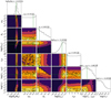 |
Fig. B.3 Posterior probability distributions of the model parameters for a simulated observation of the no-cloud atmospheric configuration at S∕N = 10. The planetary radius is considered unconstrained. Green lines mark the true values of the model parameters (see Table 2) for this observation. Two-dimensional subplots show the correlations between pairs of parameters. Contour lines correspond to the 0.5, 1, 1.5, and 2 σ levels. The median of each parameter’s distribution is shown on top of their 1D probability histogram. Upper and lower errors correspond to the 84 and 16% quantiles. |
B.4 Unknown Rp; thin-cloud scenario
B.5 Unknown Rp; thick-cloud scenario
Appendix C Retrieval results for different noise realizations
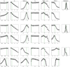 |
Fig. C.1 Solid black lines: marginalized probability distributions for each of the model parameters, given in each of the columns, after performing the retrievals ten times for as many different noise realizations of the measured spectra. Top rows: no-cloud scenario, both for Rp unknown and known. Middle rows: thin-cloud scenario, both for Rp unknown and known. Bottom rows: thick-cloud scenario, both for Rp unknown and known. Vertical green lines mark the true values of the model parameters (see Table 2) for each scenario. |
References
- Ackerman, A. S., & Marley, M. S. 2001, ApJ, 556, 872 [NASA ADS] [CrossRef] [Google Scholar]
- Barnard, E. 1916, AJ, 29, 695 [Google Scholar]
- Barros, S. C. C., Gosselin, H., Lillo-Box, J., et al. 2017, A&A, 608, A25 [NASA ADS] [CrossRef] [EDP Sciences] [Google Scholar]
- Batalha, N. E., Smith, A. J. R. W., Lewis, N. K., et al. 2018, ApJ, 156, 158 [CrossRef] [Google Scholar]
- Bevington, P. R., & Robinson, D. K. 2003, Data reduction and error analysis for the physical sciences (McGraw Hill, New York, USA) [Google Scholar]
- Bolcar, M. R., Feinberg, L., France, K., et al. 2016, Proc. SPIE, 9904, 99040J [CrossRef] [Google Scholar]
- Borucki, W.J., & Summers, A. L. 1984, Icarus, 58, 121 [NASA ADS] [CrossRef] [Google Scholar]
- Buenzli, E., & Schmid, H. M. 2009, A&A, 504, 259 [NASA ADS] [CrossRef] [EDP Sciences] [Google Scholar]
- Cahoy, K. L., Marley, M. S., & Fortney, J. J. 2010, ApJ, 724, 189 [NASA ADS] [CrossRef] [Google Scholar]
- Damiano, M., & Hu, R. 2019, AJ, 159, 175 [CrossRef] [Google Scholar]
- D’Angelo, G., & Bodenheimer, P. 2013, ApJ, 778, 77 [NASA ADS] [CrossRef] [Google Scholar]
- Dawson, P. C., & De Robertis, M. M. 2004, AJ, 127, 2909 [NASA ADS] [CrossRef] [Google Scholar]
- Dlugach, J. M., & Yanovitskij, E. G. 1974, Icarus, 22, 66 [NASA ADS] [CrossRef] [Google Scholar]
- Fabrycky, D. C., Lissauer, J. J., Ragozzine, D., et al. 2014, ApJ, 790, 146 [Google Scholar]
- Feng, Y. K., Robinson, T. D., Fortney, J. J., et al. 2018 AJ, 155, 200 [NASA ADS] [CrossRef] [Google Scholar]
- Foreman-Mackey, D., Hogg, D. W., Lang, D., & Goodman, J. 2013, PASP, 125, 306 [CrossRef] [Google Scholar]
- García Muñoz, A., & Cabrera, J. 2018, MNRAS, 473, 1801 [NASA ADS] [CrossRef] [Google Scholar]
- García Muñoz, A., & Isaak, K. G. 2015, PNAS, 112, 44 [Google Scholar]
- García Muñoz, A., & Mills, F. P. 2015, A&A, 573, A72 [NASA ADS] [CrossRef] [EDP Sciences] [Google Scholar]
- García Muñoz, A., Zapatero Osorio, M. R., Barrena, R., et al. 2012, ApJ, 755, 103 [NASA ADS] [CrossRef] [Google Scholar]
- García Muñoz, A., Pérez-Hoyos, S., & Sánchez-Lavega, A. 2014, A&A, 566, L1 [NASA ADS] [CrossRef] [EDP Sciences] [Google Scholar]
- García Muñoz, A., Lavvas, P., & West, R. A. 2017, Nat. Astron., 1, 0114 [CrossRef] [Google Scholar]
- Gatewood, G., & Eichhorn, H. 1973, AJ, 78, 769 [NASA ADS] [CrossRef] [Google Scholar]
- Giampapa, M. S., Rosner, R., Kashyap, V., et al. 1996, ApJ, 463, 707 [NASA ADS] [CrossRef] [Google Scholar]
- Goodman, J., & Weare, J. 2010, Comm. App. Math. Comp. Sci., 5, 65 [Google Scholar]
- Greco, J. P., & Burrows, A. 2015, ApJ, 808, 172 [CrossRef] [Google Scholar]
- Guimond, C. M., & Cowan, N. B. 2018, AJ, 155, 230 [CrossRef] [Google Scholar]
- Heindinger, A.K., & Stephens, G. L. 2000, JAS, 57, 1615 [Google Scholar]
- Helling, Ch., Tootill, D., Woitke, P., & Lee, G. 2017, A&A, 603, A123 [NASA ADS] [CrossRef] [EDP Sciences] [Google Scholar]
- Horak, H. G. 1950, ApJ, 112, 445 [NASA ADS] [CrossRef] [Google Scholar]
- Hu, R. 2019, ApJ, 887, 166 [CrossRef] [Google Scholar]
- Ida, S., & Lin,D. N. C. 2008, ApJ, 685, 584 [NASA ADS] [CrossRef] [Google Scholar]
- Ikoma, M., Emori, H., & Nakazawa, K. 2001, ApJ, 553, 999 [NASA ADS] [CrossRef] [Google Scholar]
- Ilic, N., García Muñoz, A., Benoît, S., et al. 2018, EPSC Abstracts, EPSC2018-745 [Google Scholar]
- Inaba, S., & Ikoma, M. 2003, A&A, 410, 711 [NASA ADS] [CrossRef] [EDP Sciences] [Google Scholar]
- Karkoschka, E. 1994, Icarus, 111, 174 [NASA ADS] [CrossRef] [Google Scholar]
- Lacy, B., Shlivko, D., & Burrows, A. 2019, AJ, 157, 132 [CrossRef] [Google Scholar]
- Lupu, R. E., Marley, M. S., Lewis, N., et al. 2016, AJ, 152, 217 [CrossRef] [Google Scholar]
- Madhusudhan, N., & Seager, S. 2009, ApJ, 707, 24 [NASA ADS] [CrossRef] [Google Scholar]
- Marois, C., Doyon, R., Racine, R., & Nadeau, D. 2000, PASP, 112, 767 [Google Scholar]
- Mennesson, B., Gaudi, S., Seager, S., et al. 2016, Proc. SPIE, 9904, 99043H [CrossRef] [Google Scholar]
- Mishchenko, M. I. 1989, Icarus, 84, 296 [NASA ADS] [CrossRef] [Google Scholar]
- Misra, A., Meadows, V., & Crisp, D. 2014, ApJ, 792, 61 [CrossRef] [Google Scholar]
- Morozhenko, A. V., & Yanovitskij, E. G. 1973, Icarus, 18, 583 [NASA ADS] [CrossRef] [Google Scholar]
- Nayak, M., Lupu, R., Marley., Fortney, J. J. et al. 2017, PASP, 129, 973 [CrossRef] [Google Scholar]
- Ohno, K., & Okuzumi, S. 2017, ApJ, 835, 261 [NASA ADS] [CrossRef] [Google Scholar]
- Pérez-Hoyos, S., Sanz-Requena, J. F., Barrado-Izaguirre, N., et al. 2012, Icarus, 217, 256 [NASA ADS] [CrossRef] [Google Scholar]
- Pierrehumbert, R., & Gaidos, E. 2011, ApJ, 734, L13 [NASA ADS] [CrossRef] [Google Scholar]
- Press, W. H., Teukolsky, S. A., Vetterling, W. T., & Flannery, B. P. 2007, Numerical Recipes: The art of Scientific Computing (Cambridge, UK: Cambridge University Press) [Google Scholar]
- Rauer, H., Catala, C., Aerts, C., et al. 2014, Exp. Astron., 38, 249 [NASA ADS] [CrossRef] [Google Scholar]
- Ribas, I., Tuomi, M., Reiners, A., et al. 2018, Nature, 563, 365 [NASA ADS] [CrossRef] [Google Scholar]
- Robinson, R. D., Stapelfeldt, K. R., & Marley, M. S. 2016, PASP, 128, 025003 [CrossRef] [Google Scholar]
- Sánchez-Lavega, A. 2010, An introduction to planetary atmospheres (Boca Raton, USA: CRC Press) [CrossRef] [Google Scholar]
- Sánchez-Lavega, A., Pérez-Hoyos, S., & Hueso, R. 2004, Am. J. Phys., 72, 767 [NASA ADS] [CrossRef] [Google Scholar]
- Satoh, T., Itoh, S., Kawabata, K., et al. 2000, PASJ, 52, 363 [CrossRef] [Google Scholar]
- Schmid, H. M., Buenzli, F. J. E., & Gisler, D. 2011, Icarus, 212, 701 [NASA ADS] [CrossRef] [Google Scholar]
- Schmitt, J. H. M. M., & Liefke, C. 2004, A&A, 417, 651 [NASA ADS] [CrossRef] [EDP Sciences] [Google Scholar]
- Smith, P. H., & Tomasko, M. G. 1984, Icarus, 58, 35 [NASA ADS] [CrossRef] [Google Scholar]
- Spergel, D., Gehrels, N., Breckinridge, J., et al. 2013, ArXiv e-prints [arXiv:1305.5422] [Google Scholar]
- Spergel, D., Gehrels, N., Baltay, C., et al. 2015, ArXiv e-prints [arXiv:1503.03757] [Google Scholar]
- Stark, C. C., Roberge, A., Mandell, A., et al. 2015, ApJ, 808, 149 [NASA ADS] [CrossRef] [Google Scholar]
- Stephens, G. L., & Heindinger, A. K. 2000, JAS, 57, 1599 [Google Scholar]
- Tal-Or, L., Zucker, S., Ribas, I., Anglada-Escudé, G., & Reiners, A. 2019, A&A, 623, A10 [NASA ADS] [CrossRef] [EDP Sciences] [Google Scholar]
- The LUVOIR Team 2018, ArXiv e-prints [arXiv:1809.09668] [Google Scholar]
- Trauger, J., Moody, D., Krist, J., & Gordon, B. 2016, JATIS, 2, 011013 [Google Scholar]
- van de Kamp, P. 1963, AJ, 68, 515 [NASA ADS] [CrossRef] [Google Scholar]
- Virtanen, P., Gommers, R., Oliphant, T. E., et al. 2020, Nat. Methods, 17, 261 [Google Scholar]
- von Paris, P., Hedelt, P., Selsis, F., Schreier, F., & Trautmann, T. 2013 A&A, 551, A120 [NASA ADS] [CrossRef] [EDP Sciences] [Google Scholar]
- Wahhaj, Z., Cieza, L. A., Mawet, D., et al. 2015, A&A, 581, A24 [NASA ADS] [CrossRef] [EDP Sciences] [Google Scholar]
- Zeng, L., Jacobsen, S. B., Sasselov, D. D., et al. 2019, PNAS, 116, 20 [CrossRef] [Google Scholar]
All Tables
Values for the parameters in the atmospheric vector p used to construct the grid of synthetic reflected-starlight spectra.
All Figures
|
Fig. 1 Sketch of the vertical structure in our atmospheric model. ILAY denotes each of the slabs into which the atmosphere is divided, each with thickness Hg ∕2. Gas density decreases exponentially with height. The atmosphere is assumed to contain CH4, with a certain fraction |
| In the text | |
|
Fig. 2 Scattering phase functions for the considered values of reff. |
| In the text | |
|
Fig. 3 Solid black lines: synthetic spectra for the thin-cloud configuration (see Table 2). Coloured lines: synthetic spectra for the configurations that result from perturbing each of the elements of the six-dimensional atmospheric vector p = {τc, Δc, τc →TOA, reff, ω0,
|
| In the text | |
|
Fig. 4 Solid lines: true (noiseless) spectra for the three atmospheric configurations in Table 2 at phase angle α = 0°. Symbols: corresponding measured spectra, with error bars specific to S∕N = 10. The size of the error bars (σm; see text) is defined on the basis of the brightest spectral bin (which typically occurs near 500 nm) and is the same at all wavelengths for each spectrum. The spectra correspond to no-cloud (light blue), thin-cloud (dark blue), and thick-cloud (purple) atmospheric configurations. |
| In the text | |
|
Fig. 5 Solid green line: true spectrum for the true atmospheric configuration. Red symbols: simulated measured spectrum, with error bars corresponding to S∕N = 10. Solid black lines: synthetic spectra that meet the condition Δχ2 < 15.1, generated during the MCMC retrieval for a known Rp. Top: no-cloud configuration; middle: thin-cloud; bottom: thick-cloud. |
| In the text | |
|
Fig. 6 Posterior probability distributions of the model parameters for a simulated observation of the no-cloud atmospheric configuration at S∕N = 10. The planetary radius is assumed to be known and Rp∕RN = 0.6. Green lines mark the true values of the model parameters (see Table 2) for this observation. Two-dimensional subplots show the correlations between pairs of parameters. Contour lines correspond to the 0.5, 1, 1.5, and 2σ levels. The median of each parameter’s distribution is shown on top of their 1D probability histogram. Upper and lower uncertainties correspond to the 84 and 16% quantiles. The figures corresponding to the other scenarios discussed in Sects. 4.1 and 4.2 are shown in Appendix B. |
| In the text | |
|
Fig. 7 As Fig. 5, but for retrievals where the planetary radius is unknown. Top: no-cloud configuration; middle: thin-cloud; bottom: thick-cloud. |
| In the text | |
|
Fig. 8 Black line: synthetic spectrum for the thin-cloud configuration (Table 2). Colour lines: synthetic spectra for the configurations that result from perturbing Rp ∕RN. The colour code is described in the legend for the lowermost and uppermost values. Intermediate colours span over the values Rp∕RN = {0.40, 0.50, 0.60, 0.70, 0.80}. This corresponds to a radius uncertainty of ΔRp = 33%. |
| In the text | |
|
Fig. 9 Marginalized probability distributions for τc
(top) and |
| In the text | |
|
Fig. A.1 Top: distribution of var values for the 1000 random realizations selected to compare the planetary albedo obtained by solving the multiple scattering problem and that obtained by linear interpolation from the grid. Bottom: computed (solid green line) and interpolated (dashed red line) albedos for the configuration with the highest var value. |
| In the text | |
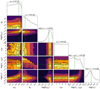 |
Fig. B.1 Same as Fig. 6, but for the thin-cloud scenario (see Table 2). |
| In the text | |
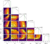 |
Fig. B.2 Same as Fig. 6, but for the thick-cloud scenario (see Table 2). |
| In the text | |
|
Fig. B.3 Posterior probability distributions of the model parameters for a simulated observation of the no-cloud atmospheric configuration at S∕N = 10. The planetary radius is considered unconstrained. Green lines mark the true values of the model parameters (see Table 2) for this observation. Two-dimensional subplots show the correlations between pairs of parameters. Contour lines correspond to the 0.5, 1, 1.5, and 2 σ levels. The median of each parameter’s distribution is shown on top of their 1D probability histogram. Upper and lower errors correspond to the 84 and 16% quantiles. |
| In the text | |
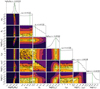 |
Fig. B.4 Same as Fig. B.3, but for a thin-cloud scenario (see Table 2). |
| In the text | |
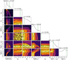 |
Fig. B.5 Same as Fig. B.3, but for a thick-cloud scenario (see Table 2). |
| In the text | |
|
Fig. C.1 Solid black lines: marginalized probability distributions for each of the model parameters, given in each of the columns, after performing the retrievals ten times for as many different noise realizations of the measured spectra. Top rows: no-cloud scenario, both for Rp unknown and known. Middle rows: thin-cloud scenario, both for Rp unknown and known. Bottom rows: thick-cloud scenario, both for Rp unknown and known. Vertical green lines mark the true values of the model parameters (see Table 2) for each scenario. |
| In the text | |
Current usage metrics show cumulative count of Article Views (full-text article views including HTML views, PDF and ePub downloads, according to the available data) and Abstracts Views on Vision4Press platform.
Data correspond to usage on the plateform after 2015. The current usage metrics is available 48-96 hours after online publication and is updated daily on week days.
Initial download of the metrics may take a while.