| Issue |
A&A
Volume 633, January 2020
|
|
|---|---|---|
| Article Number | A92 | |
| Number of page(s) | 14 | |
| Section | The Sun | |
| DOI | https://doi.org/10.1051/0004-6361/201936832 | |
| Published online | 16 January 2020 | |
Determining whether the squashing factor, Q, would be a good indicator of reconnection in a resistive MHD experiment devoid of null points
1
School of Mathematics and Statistics, University of St Andrews, St Andrews, Fife KY16 9SS, UK
e-mail: jr93@st-andrews.ac.uk, cep@st-andrews.ac.uk
2
Jodrell Bank Centre for Astrophysics, School of Physics and Astronomy, University of Manchester, Manchester M13 9PL, UK
Received:
2
October
2019
Accepted:
21
November
2019
The squashing factor of a magnetic field, Q, is commonly used as an indicator of magnetic reconnection, but few studies seek to evaluate how reliable it is in comparison with other possible reconnection indicators. By using a full, self-consistent, three-dimensional, resistive magnetohydrodynamic experiment of interacting magnetic strands constituting a coronal loop, Q and several different quantities are determined. Each is then compared with the necessary and sufficient condition for reconnection, namely the integral along a field line of the component of the electric field parallel to the magnetic field. Among the reconnection indicators explored, we find the squashing factor less successful when compared with alternatives, such as Ohmic heating. In a reconnecting magnetic field devoid of null points, our work suggests that Q, being a geometric measure of the magnetic field, is not a reliable indicator of the onset or a diagnostic of the location of magnetic reconnection in some configurations.
Key words: Sun: corona / Sun: magnetic fields / magnetic reconnection / magnetohydrodynamics (MHD)
© ESO 2020
1. Introduction
One of the key physical plasma processes playing a major role in dynamic events on the Sun, in other stars, in the magnetosphere, and in laboratory experiments is magnetic reconnection (Priest & Forbes 2000; Zweibel & Yamada 2016). It is a known driver of solar and stellar flares (e.g. Carmichael 1964; Sturrock 1966; reviewed by Pontin 2012), is likely to be involved in heating solar and stellar coronae, as well as accretion discs (e.g. Ross & Latter 2018), and also plays a role in dynamic ejecta, such as coronal mass ejections and jets (e.g. Archontis & Hood 2013; Raouafi et al. 2016). In the magnetosphere, the interaction and subsequent reconnection of the magnetic solar wind and the different connectivities of the Earth’s magnetic field, on both the dayside and the nightside, are important for triggering substorms, for causing aurora, and for creating flux transfer events (e.g. Dungey 1961; Hones 1979; Wright 1987; Phan et al. 2016). Both large-scale plasma physics experiments, such as the International Thermonuclear Experimental Reactor (ITER) and the Joint European Torus (JET), and small-scale experiments, such as the Small Tight Aspect Ratio Tokamak (START) and Mega Ampere Spherical Tokamak (MAST), involve reconnection (e.g. Stanier et al. 2013; McClements 2019). In several cases, reconnection is key to the initial creation of the isolated plasma.
In order to understand the behaviour of the plasma systems mentioned above, three-dimensional models are used. These models study either the complete system or a part of it, through potential or magnetohydrostatic (MHS) equilibria (e.g. Low 1985; Bogdan & Low 1986; Neukirch 1995), complex numerical magnetohydrodynamic (MHD) simulations (e.g. Galsgaard & Nordlund 1996; Bingert & Peter 2011), multi-fluid simulations (e.g. Yamada 2010), or particle-in-cell (PIC) experiments (e.g. Baumann & Nordlund 2012). In order to analyse reconnection in these systems, it is useful to determine the sites at which magnetic reconnection takes place. Over many years, a host of different approaches have been employed, depending upon the modelling undertaken. When modelling involves only two-dimensional magnetic systems, identifying the sites of reconnection is relatively straightforward: these must be X-type null points, since, in two dimensions, these are the only locations at which reconnection can occur, as discussed in detail by Priest & Forbes (2000). In three dimensions, however, reconnection is much more varied and may occur not only at magnetic null points, but also away from such locations (Vasyliunas 1984; Schindler et al. 1988; Priest & Forbes 2000).
Three-dimensional magnetic systems involving null points offer the possibility of finding the magnetic skeleton of the field, which is composed of null points, their associated spine lines, separatrix surfaces, and connecting separators. These have been found in various numerical experiments to be locations where current sheets form and subsequent reconnection occurs (Haynes et al. 2007; Haynes 2008; Wyper & Pontin 2014). In the absence of any null points, and in view of the difficulty in finding the magnetic skeleton even where one can isolate the null points, many authors have instead chosen to calculate the squashing factor (e.g. Aulanier et al. 2006; Démoulin 2007). The quantity Q, sometimes known as the quasi-squashing factor, is a quantitative measure of the degree to which initially neighbouring field lines diverge as they traverse a system (Priest & Démoulin 1995; Titov et al. 2002). In the presence of null points, separators connecting oppositely signed pairs are readily inferred: here, there is a discontinuity in the field line mapping by which reconnection is identified (e.g. Parnell et al. 2010). Priest & Démoulin (1995) and Démoulin et al. (1996a) generalize from the definitive notion of separators to that of quasi-separatrix layers (QSLs), regions of significant, yet continuous, deformation of field lines without null points. They propose to identify these where the gradients of the field line mapping are very large. Titov et al. (2002) adapt this definition to formulate the squashing factor, Q, and suggest that regions of high Q are likely sites for reconnection. Recently, Boozer (2019) emphasizes the role of exponential separation of field lines in three-dimensional geometries in allowing for fast reconnection.
Since its conception, the squashing factor has seen extensive use as an identifier and measure of reconnection (as elaborated by Janvier 2017). Longcope & Strauss (1994) illustrate the viability of the formation of electric currents on QSLs. In solar physics, its popularity is partly on account of its being inferable from magnetograms. The formation of electric currents and the consequent capacity for reconnection have been noted in analytic models of QSLs (e.g. Titov et al. 2003) and on broad, pre-existing QSLs in numerical simulations (e.g. Galsgaard et al. 2003; Milano et al. 1999). Aulanier et al. (2005) find evidence of precisely such a connection between reconnection and Q in specific steady, and thus not time-dependent, configurations, and they demonstrate narrow current layers more generally at QSLs. In the presence of null points, reconnection has been noted to be embedded within QSLs, where intense currents can accumulate (Masson et al. 2009). Maclean et al. (2009) find a relationship Q and E∥ in fields that are generated from magnetograms and subject to a slow shearing. Moreover, De Moortel & Galsgaard (2006a,b) find evidence of rotating or spinning the footpoints of coronal loops leading to QSLs that are candidate sites for reconnection, and are associated with the creation of strong current layers; the precise configuration of these is determined by the nature of the footpoint motions applied. It has, indeed, been argued that, although QSLs and strong currents need not be linked in general, they are more likely to occur together under the action of boundary motions (as argued by Tassev & Savcheva 2017). Modelling of such boundary motions introduces a new perspective since they are typically treated in models between two parallel photospheric planes, which contrasts with the configuration in which the squashing factor was originally formulated, that assumed field lines mapping from one part to another of a single plane, across a polarity inversion line. However, the mathematical composition remains identical. With particular regard to models of line-tied coronal flux tubes, the two conceived parts equally represent part of one single physical solar surface; their being parallel removes additional effects caused by curvature.
Observations of solar phenomena provide evidence of such a link between squashing of the magnetic field and reconnection. Reconnection at QSLs or hyperbolic flux tubes (HFTs), alongside topological features, clearly occurs, providing some of the observed particle acceleration from ribbons and the associated strong emission (Reid et al. 2012). Indeed, the extrapolations of the fields around flares have shown high-Q regions without null points, which results give strong evidence of their role in reconnection (e.g. Mandrini et al. 2006). Far more limited has been the examination of Q with respect to field-line-integrated parallel electric field, ∫ E∥ ds. Maclean et al. (2009) demonstrate correlation of the two in reconnecting fields with null points, although this is established visually and not quantitatively. Wilmot-Smith et al. (2009, 2010) find QSLs existing away from active sites of reconnection, and argue that the nature of their relationship with reconnection is not clear, in line with the similar work of Restante (2011). Should it be possible to establish a link between the two, it has been suggested, in turn, to be a contributing factor for heating and particle acceleration (Démoulin & Priest 1997; Aulanier et al. 2006). As discussed above, QSLs, undoubtedly, are documented to be able to host reconnection, and tentative evidence agrees that they may be then linked with the occurrence of solar flares (Démoulin et al. 1996b, 1997). Nevertheless, little in existing literature compares Q and ∫ E∥ ds in a globally non-null magnetic field. Wendel et al. (2013) find “excellent agreement”, in a kinetic simulation of generic reconnection, between the boundaries of quasi-potential Ξ = −∫α, β E∥ ds and the QSL. In laboratory plasma, reconnection can occur at sites where Q is high and currents are created. QSLs exist in reconnecting laboratory flux ropes (Gekelman et al. 2010, 2012); likewise, Gekelman et al. (2016) identify high Q associated with a reconnecting current sheet, yet remark even higher subsequent values of Q not linked with any reconnection, suggesting that any relationship is subtle and complicated.
Whilst it has been previously often suggested that regions of high Q are likely sites of reconnection in the presence of driving flows, no rigorous quantitative link has been established between Q and reconnection locations. Here, for the first time, we provide a statistical analysis between the various potential indicators of reconnection, including Q and Ohmic heating. In order to investigate this, it is necessary to use three-dimensional MHD simulations, since both dynamics and three-dimensional fields are essential in order to have reconnection and for Q to play a role. Similarly to the work of De Moortel & Galsgaard (2006a,b), we have considered reconnection within modelled coronal loops subject to boundary motions. We investigated the conditions in which Q foresees reconnection in braided magnetic fields arising from driving flows. We studied the distribution of the localized instances of reconnection and analysed their nature. Such forms of driven reconnection are likely to contribute, at least in some measure, to the heating necessary in the solar atmosphere (Parnell & Galsgaard 2004).
In order to understand the locations of magnetic reconnection, and the validity of different indicators of reconnection in fields of simple topology, without null points, we utilized the magnetic field configuration studied in the previous paper, Reid et al. (2018; hereafter, Paper I). This field begins with a simple configuration of initially straight field lines, which, under the action of simple and ordered boundary motions, develops a complex pattern of multiple instances of reconnection. Building on preceding studies of the kink instability in coronal loops, which Browning et al. (2008) and Hood et al. (2009) show capable of triggering instability and subsequent release of magnetic energy, the model demonstrably leads to the formation of fragmentary structures in current. Instability and reconnection then spread among neighbouring threads, as in the generalization to several strands of Tam et al. (2015) and Hood et al. (2016).
In Sect. 2, we sketch the model studied here, and in Sect. 3 the broad evolution. Then, in Sect. 4, we seek to analyse the onset and occurrence of reconnection in that numerical experiment. In Sect. 5, we determine and compare several prospective indicators of reconnection. Finally, we draw conclusions in Sect. 6.
2. Set-up of numerical experiment
The model is the same as in Paper I; it consisted of a uniform, vertical magnetic field, to which three rotational driving motions were applied, in opposing senses on each z boundary, in order to create three separate, distinct strands (“threads”: twisted regions of magnetic field) between footpoints fixed in each of two plane-parallel photospheric boundaries. These driving motions were continued throughout the course of the experiment. The two parallel boundary planes give natural planes that are subsequently used in calculating Q, but this is distinct from single-plane models mapping one part of a plane to another.
2.1. Numerical method
The dimensionless equations of fully three-dimensional magnetohydrodynamics (MHD) were solved, using the Lare3d code (Arber et al. 2001):
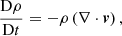
where ρ is mass density, v plasma velocity, B magnetic field, P gas pressure, Fshock the shock viscosities, Fvisc. a uniform viscous force, η = 1/σ the dimensionless magnetic resistivity (given conductivity σ; the dimensionless vacuum permeability is μ0 = 1), ε = P/ρ(γ−1) the specific internal energy (where γ = 5/3 is the ratio of specific heats), j current density, and Qvisc. the combined viscous heating. The uniform viscosity is implemented with a Laplacian operator acting on velocity,
given coefficient of dynamic viscosity μ. The system’s volume, of dimensions −3 ≤ x, y ≤ 3 and −10 ≤ z ≤ 10, was discretized on a computational grid of 5122 × 2048 cells. These non-dimensional forms for the equations follow from the specification of a normalizing length L0, mass density ρ0, and magnetic field B0. Thus, there are reference Alfvén speed  , Alfvén time tA = L0/vA, energy density
  , current density j0 = B0/(μ0 L0), and electric field
  .
.
The boundary conditions in z were a photospheric driving velocity and zero-gradient for the remaining quantities. The side boundaries were periodic for all quantities. In terms of the normalization discussed above, the initial conditions comprised a plasma of uniform density and specific internal energy, ρ = 1 and ε = 0.1, in a uniform vertical magnetic field B = 1ez. There were no null points, initially or at any time subsequently. The initial plasma beta of 2/15, being less than unity, indicates that magnetic forces dominate. The full configuration and parameters of the model are detailed in Paper I.
2.2. Driving velocity
The spatial form for the driver is provided by:
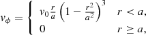
which was applied at three points, (−2,0), (0,0), and (2,0), around which the radial coordinate, r, is locally defined, in regions of fixed radius a = 1. The coefficient v0, which regulates the speed of driving, was chosen such that the threads are respectively driven with maximum speeds 0.02, 0.05, and 0.02.
2.3. Resistivity model
Realistic coronal magnetic Reynolds numbers are not presently computational viable, on account of the extremely short length scales that would then need to be resolved. In order to match the near-ideal nature of a coronal plasma as closely as is possible, we used zero uniform (background) resistivity. However, in order to study reconnection, the electric field must be calculated, which precludes relying on numerical dissipation. Therefore, an anomalous resistivity was applied above a certain threshold on the magnitude of total current density, jcrit..
The resistivity was accordingly prescribed by
In order to determine an appropriate current threshold, an experiment was conducted with only numerical diffusion. Within that numerical experiment, the imposed driving motions created three twisted threads; in the most rapidly driven central thread, a kink instability formed, provoking reconnection and the onset of avalanche-like behaviour. The threshold on current, jcrit., was chosen from that experiment, such that, in the main study, the build-up of current during the initial linear phase of the evolution should not be inhibited and the central thread would attain marginal instability prior to the onset of reconnection. The level chosen was jcrit. = 5.0, and the anomalous resistivity was fixed at η0 = 10−3.
Our chosen model makes both resistivity and, consequently, the parallel electric field highly localized, which is physically apt: resistivity is not uniform. Plasma physics experiments have found it to be enhanced within localized regions of strong current, where length scales are of the order of a few ion inertial lengths (Cairns 1985). Within such regions, micro-instabilities generate turbulence, which disrupts the flow of electrons and causes a rise of several orders of magnitude in resistivity. In general, in coronal plasma, η is so low as to be negligible, and only under certain conditions, achieved in localized regions, does it reach a material level, here reflected by the anomalous “switch-on”. Equally, this anomalous resistivity is motivated by resembling, on a finite grid, the collapse, given hypothetically infinite resolution, of length scales to a level at which classical resistivity would act.
3. Dynamic evolution under continued driving
The driven three-dimensional numerical experiment studied here proceeds as follows. In the initial phase of development, continuous driving motions cause the initially uniform field to form three distinct, helically twisted threads, while injecting a Poynting flux that increases the magnetic energy of the system. When the central thread, which is most rapidly driven, attains sufficient twist, marginal instability is reached and an helical current sheet forms (t ≈ 175). The ensuing kink instability in the central thread instigates an avalanche of reconnection events that first disrupt the right-hand thread: the two threads expand and flow together, sharp currents emerge between them, they reconnect with each other, and the self-twisted flux tubes establish a mutual helicity over the combined structure. Evidence suggests that this occurs before this right-hand thread is kink-unstable. The left-hand thread remains, at this time, unperturbed by the ensuing avalanche and continues to be twisted by the boundary motions. At t = 275, there are indications that this thread is nearing marginal stability; it, too, is then disrupted in the avalanche. The first instability, and consequent effects on the second and third threads, are associated with large heating events, during which significant magnetic energy is converted into kinetic energy and dissipated directly by Ohmic heating. Thereafter, as driving continues, smaller, widely distributed heating events, associated with substantially smaller current sheets, recur. Thus, this experiment involves numerous reconnection events that occur on a wide range of scales, and continue unabated from approximately t = 175 onwards. None of these events are associated with null points, separators, or other topological features, as all the field lines remain largely vertical throughout the experiment. Hence, this numerical experiment is an instructive scenario in which to consider the association between the squashing factor Q, other potential identifiers, and actual sites of reconnection.
4. Occurrence of magnetic reconnection
As discussed earlier, the resistivity of coronal plasma is, in general, very small everywhere except within highly localized regions. A necessary and sufficient condition to identify the location and occurrence of three-dimensional reconnection is
where s parameterizes the distance along a field line (Schindler et al. 1988; Hesse & Schindler 1988).
Indeed, ∫ E∥ ds is, in fact, everywhere non-zero in a plasma, since classical resistivity is very small but non-zero, even in regions of approximately ideal MHD. When stated to be non-zero, it is intended that this integral is significantly larger than it is on a field line threading only these near-ideal MHD regions (Parnell et al. 2018).
The integral in Eq. (8) is calculated starting from the mid-plane (z = 0), through which all field lines are assumed to pass. Starting points (xi,yj, 0) are uniformly distributed over the grid in that plane. From there, field lines are traced in both directions, both forwards and backwards, and the parallel electric field, E∥ = ηj∥ (cf. Eq. (9) below), integrated along them. For each time, a total of 5132 field lines are integrated.
Contours of ∫ E∥ ds, calculated from these points in the mid-plane, are shown in Fig. 1 for six times. Those for the first two times demonstrate the beginning of the reconnection associated with the initial kink instability in the central thread (t = 175, Fig. 1a) and its aftermath (t = 200, Fig. 1b), when evidence of reconnection has spread throughout the central thread’s cross-sectional area. Fig. 1c at t = 225 shows evidence of reconnection having extended to the right thread, which has become completely engulfed by reconnection at t = 275. At this time, there is also evidence in the left-hand thread of reconnection, possibly triggered by a kink instability. This thread is then shown to be affected by reconnection across its entire cross-section, both by its instability and by the growing unstable region to its right (t = 325, Fig. 1e). The aftermath of the disruption of all three threads at t = 400 (Fig. 1f) reveals that reconnection is over a wide-spread area, much larger than that covered by the driven region on the top and bottom boundaries. These reconnection events continue, although their spatial locations and properties change throughout the rest of the experiment.
 |
Fig. 1. Contours of the field-line-integrated parallel electric field, plotted where field lines intersect the mid-plane. Times shown are (a) t = 175, (b) t = 200, (c) t = 225, (d) t = 275, (e) t = 325, and (f) t = 400. Times (b), (e), and (f) are subsequently considered in greater detail. In (a), the dashed black lines indicate the radii of the driven regions, representing footpoints of the left, central, and right threads. The contours are shaded according to the logarithmic scale on the colour bar. |
Within the several snapshots in Fig. 1, there are regions of both positive and negative field-line-integrated parallel electric field. These persist throughout the experiment, with the regions of negative ∫ E∥ ds originating in the centre of the twisted threads and the positive regions originating in the outer rings. It is clear that |∫ E∥ ds| is larger in regions where ∫ E∥ ds > 0 than where ∫ E∥ ds < 0, although the data show a comparable number of points where the integral is positive and negative. By taking the component of Ohm’s law parallel to the magnetic field,
Thus, the sign of E∥ is dependent on the direction of the electric current relative to the magnetic field. In the early phase of the experiment, the magnetic field in a single thread, in cylindrical coordinates, has a poloidal component of the same spatial form as the driving velocity and an axial component from the initial vertical field. It can be calculated using the ideal induction equation:
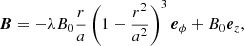
where

(cf. Paper I). The correction to the z-component is 𝒪(λ2). Associated with this magnetic field is a vertical electric current,
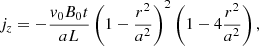
which changes sign at r = a/2. The kink instability forms a current sheet at the mode-rational surface r = rm, where
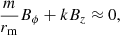
(e.g. Bateman 1978; Hood & Priest 1979). Here, m = 1 is the mode number for the kink mode, and we consider  as the axial wave number. Thus,
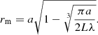
At marginal instability, we approximate λ = 1.586 (more fully discussed in Reid et al. 2018), which yields rm ≈ 0.73 > 0.5. Accordingly, the current sheet associated with the kink instability emerges where the current is mainly in the positive z-direction. Hence, instability occurs where E∥ is similarly positive. Notwithstanding this, as is obvious in Fig. 1, reconnection does occur in which E∥ < 0, likely proceeding from reconnection after the kink instability near the centres of threads, where parallel current is negative.
Figure 2 shows, at time t = 200, a sample of field lines in three dimensions, coloured according to ∫ E∥ ds (Fig. 2a) and, separately, according to the current along each field line (Fig. 2b). As expected in a plasma with a high magnetic Reynolds number, the current along a field line only breaches the threshold necessary to trigger reconnection in small, localized regions, and so ∫ E∥ ds is only non-zero in such confined regions. It is seen that strong current, associated with current layers, cannot be of great spatial extent, nor can it persist for long. The large magnitudes of current that form the current layers are both small and short-lived, since the anomalous resistivity efficiently dissipates all such current. However, currents are continuously being build up through the twisting of the field via the driving motions.
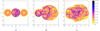 |
Fig. 2. Sample of field lines traced from the mid-plane, coloured (a) solidly according to ∫ E∥ ds and (b) parametrically according to current, |j|(s). Plots are shown at t = 200. In (a), green denotes a field line along which ∫ E∥ ds = 0. In (b), all |j| ≤ jcrit. = 5.0 is shaded blue, and current with magnitude above the critical threshold is shaded according to the colour bar. The radii of the driving regions are marked on the bottom z = −L plane. |
Similarly in three dimensions, the location at which reconnection occurs is shown in Fig. 3 by isosurfaces of the parallel electric field, E∥, found locally within the domain. In Fig. 3a, the parallel electric field and, consequently, the reconnection are intensely concentrated along an helical current sheet, as is a signature of the ideal kink mode. Such structure resembles magnetic field lines, although the two are not coincident: a sample of field lines is included to illustrate the significant difference between their behaviour and that of the current sheet, which has four distinct twists, although the field lines have fewer. In Fig. 3b (t = 200), the isosurfaces of E∥ are more numerous and generally of finer scale. However, there is still evidence of the original helical sheet seen at t = 175, although it now completes only one rotation.
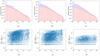 |
Fig. 3. Isosurfaces of local E∥. Times shown are (a) t = 175, (b) t = 200, (c) t = 225, (d) t = 275, (e) t = 325, and (f) t = 400. On (a) is superimposed a sample of field lines in green. The radii of the left, central, and right driving regions are marked on the bottom z = −L plane. Times (b), (e), and (f) are subsequently considered in greater detail. The isosurfaces are shaded according to the logarithmic scale on the colour bar. |
In Fig. 3c and d, reconnection sites are dispersed and dominated by smaller ones. Little, if any, evidence of the original helical current sheet persists. By t = 325 in Fig. 3, similar, albeit generally weaker, less intense, helical structures are apparent in the leftmost thread, which has been more slowly driven and contains less accumulated magnetic energy. In that thread, there are a multitude of small E∥ structures, and numerous such regions also in the central and right-hand threads. At t = 400, in Fig. 3f, any large-scale helical structure in the threads has been lost to instability and consequent reconnection. Instead, reconnection occurs almost entirely in an abundance of small-scale sites.
Reconnection, as shall also be seen in the Ohmic heating in the mid-plane, is weaker and more dispersed in these later stages. However, the perspective of Fig. 3 allows one to recognize that the reconnection remains guided by highly elongated structures.
5. Indicators of reconnection
5.1. Correlation with quasi-separatrix layers
An established trend among the work of many authors aims to predict the locations at which current sheets may emerge, and accordingly where reconnection may occur, through the gradients of the connectivity of field lines, derived from end points of neighbouring field lines (e.g. Priest & Démoulin 1995; Démoulin et al. 1996a; Aulanier et al. 2005). In order to do this, Priest & Démoulin (1995) trace field lines from points (x±,y±) on one boundary, where the subscript sign reflects the polarity of the magnetic field there. The field lines are traced until they intersect another boundary at points (X∓(x±,y±),Y∓(x±,y±)). Next, the authors use the norm of the Jacobian matrix from the mapping of field lines from one boundary to the other:
and, finally, propose that a quasi-separatrix layer (QSL) exists where

Titov et al. (2002) identify the disadvantage of such a definition, arguing that it is unsatisfactory that this measure should be non-unique for the same set of field lines, varying according to the direction traced along the field line. Hence, they formulate the quasi-squashing factor, Q, defined as

where
is the determinant of the Jacobian matrix, to eliminate this anomaly. Their definition provides a unique measure of Q, independent of the direction in which field lines are traced. Titov et al. (2002) describe a QSL as any region such that Q ≫ 2 (as geometric arguments make the minimum possible value 2). Furthermore, the numeric calculation of Q is simplified by the observation of Titov (2007) that Δ could equivalently be determined as
as a consequence of flux conservation. The quasi-squashing factor, Q, has now become one of the most common factors used to indicate the locations of reconnection.
For the results of the present numerical experiment, we have calculated Q in the mid-plane, from the points from which field lines were traced to determine ∫ E∥ ds. In order to verify the accuracy of Q for each field line, we have calculated its value by integrating along the field lines starting both from the bottom and from the top boundaries. Any attempt numerically to find the squashing factor in a magnetic field must be done advisedly, in view of several sources of error that arise. The magnetic field on a finite numerical grid is confined by resolution, with an error proportional to the square of the grid spacing. In addition to this, evaluation of the relevant gradients across such a grid by finite differencing introduces an error of second order in step size and consequent dependence on the resolution of the grid. While integration of field lines can be done with high precision, the numerical calculation of Q is limited in accuracy by the error in sub-grid interpolation. Therefore, calculation of Q, like that of ∫ E∥ ds, shows some sensitivity to the scale of the computational mesh. Since Q has two values in the mid-plane, one with respect to each boundary, there is an ambiguity in this definition (as noted by Restante 2011; Pariat & Démoulin 2012). The difference made is small, with Q similar; for consistency, we use the practice of taking the maximum value (e.g. Restante 2011).
As they are calculated from comparable grids, we can directly compare values of ∫ E∥ ds and Q in various ways. Contours of Q calculated according to this procedure are depicted in Fig. 4, at selected times so far analysed, namely t = 200, t = 325, and t = 400. Qualitatively, the contour plots in Figs. 1 and 4 resemble each other in some ways, with high Q and large ∫ E∥ ds covering similar areas and showing similar swirling patterns. However, it is not possible to assess correlation meaningfully only through such a visual comparison.
 |
Fig. 4. Quasi-squashing factor Q found in the mid-plane, at (a) t = 200, (b) t = 325, and (c) t = 400. We have taken the maximum of the values with respect to the bottom and top planes. The contours are shaded according to the logarithmic scale on the colour bar. |
In the top row of Fig. 5, histograms of the values of Q, divided according to whether ∫ E∥ ds = 0 or ∫ E∥ ds ≠ 0, are shown. These clarify the relationship which one may draw between the two: when ∫ E∥ ds = 0, indicating the total absence of reconnection, Q is very likely to be small and deformation of the magnetic field limited. On the other hand, ∫ E∥ ds ≠ 0 shows a greater range in the values of Q, the distribution more heavily focused at values which may indicate the presence of QSLs. Therefore, it appears that the fact of reconnection, but not its rate or extent, may be associated with higher Q.
 |
Fig. 5. Histograms of values of Q in the mid-plane, at (a) t = 200, (b) t = 325, and (c) t = 400; and scatter plots showing the distribution of values of Q and ∫ E∥ ds at the same point in the mid-plane, at (d) t = 200, (e) t = 325, and (f) t = 400. In order to represent the full distribution on a single set of axes, the histograms are produced with frequency density (the vertical axis) and Q (the horizontal axis) each on a logarithmic scale. The blue bars indicate the distribution where ∫ E∥ ds = 0, and the red that where ∫ E∥ ds ≠ 0. The histograms are normalized such that the two histograms for each time have a combined area of unity. The scatter plots are also produced on a logarithmic scale. |
In the bottom row of Fig. 5, values of ∫ E∥ ds are marked in scatter plots directly against the corresponding values of Q. Correlation seems weak, as the points are widely dispersed. While there appears to be some correlation, in that larger Q is generally associated with higher ∫ E∥ ds, the effect is less pronounced than it may at first appear on account of the logarithmic scaling of the axes. One can only broadly state that a low value of Q is likely to indicate the absence of reconnection, but a high value of Q is not necessarily indicative of reconnection.
5.2. Field-line-integrated parallel current
Contours of the electric current, integrated along the same field lines as are used in producing Fig. 1, are shown in Fig. 6. These closely resemble the axial current in the mid-plane plotted in Fig. 5 of Paper I, especially earlier when the current is predominantly field-aligned. Figure 6 illustrates the progression from the structure associated with the ordered driving motions, to the fragmented final state.
 |
Fig. 6. Contours of the field-line-integrated parallel electric current in the mid-plane. Times shown are (a) t = 175, (b) t = 200, (c) t = 225, (d) t = 275, (e) t = 325, and (f) t = 400, as in Figs. 1 and 3. |
Near the beginning of the experiment, before any instability, the axial current within each thread is predicted by the linearized MHD equations, in particular Eq. (12). As previously discussed, such linear predictions give a reliable indication of the initial phase of evolution in the system. For this reason, integrating along initially chiefly vertical field lines, the parallel current is most strongly negative on the axis of each thread, vanishes smoothly at r = a/2, and becomes positive further out. The behaviour is seen in the left-hand thread in the first four, and in the right-hand thread in the first three, times in Fig. 6. This simple, symmetric appearance disappears following instability and the onset of reconnection, which destroy the original structure of each thread.
The field-line-integrated parallel electric current is also used as a proxy for ∫ E∥ ds in the diagnosis and study of magnetic reconnection (e.g. Wilmot-Smith et al. 2009). Where a uniform resistivity is used, one is a linear scaling of the other, but with a non-uniform, anomalous resistivity, they differ. While the patterns and arrangement of parallel current and electric field show clear similarity (cf. Figs. 1 and 6), the former has a much greater visible structure than the latter, as expected from the critical threshold applied to resistivity in Fig. 1.
The field-line-integrated parallel current (Fig. 6) is clearly significant away from locations of reconnection, which cannot be specifically predicted using it. The truly confined, isolated nature of regions of reconnection is apparent from the field-line-integrated parallel electric field (Fig. 1), conforming to predictions about reconnection in three dimensions. In this regard, the field-aligned parallel current can only be used to study reconnection given constant, uniform resistivity.
Examining Figs. 4 and 6 (specifically, Fig. 6b, e, and f), we can compare the properties of field-line-integrated parallel current and Q. There is a certain degree of similarity in the large-scale structure. At t = 200, a thin annulus of higher Q exists around the outer edge of the central thread, where there is also a strong positive current. In the interior, there is some evidence of higher Q in small patches, particularly on the right-hand side, matching approximately some areas of dominant negative current. At t = 325, the central and right threads have merged into a single entity, with a swirling region of high Q seen around (−0.5,−1.0), where strongly negative current prevails. Similarly, there is a channel of negative current and high Q-pagination
around x = 1 between y = −1 and y = 1. The left thread at t = 325 shows, in Q and ∫ j∥ ds, a behaviour analogous to that seen earlier in the central thread. By the final time, t = 400, all three of the original threads have merged into a monolithic, disrupted structure, approximately cospatial in Q and ∫ j∥ ds. However, within this large structure, there is fine-scale structure in each quantity, but it is difficult to establish any clear correspondence between the two. Across all times, it appears to hold that strong current and elevated Q are of similar extent, containing detailed, finer features that are more difficult to correlate.
Quantitatively, Fig. 7 shows histograms of the values of ∫ j∥ ds for the two cases where ∫ E∥ ds is zero or non-zero, and scatter plots of ∫ E∥ ds against ∫ j∥ ds. As is the case for Q, the histograms reveal that where there is no reconnection, the integrated parallel current is likely to be small, and, for the first two times shown, the highest integrated parallel current values are associated with reconnection. The scatter plots show that if there is reconnection, then a broad range of values of integrated parallel current are possible.
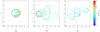 |
Fig. 7. Histograms showing the distribution of ∫ j∥ ds where the corresponding field-line-integrated parallel electric field is zero (blue) or non-zero (red) at (a) t = 200, (b) t = 325, and (c) t = 400; and scatter plots of ∫ E∥ ds against ∫ j∥ ds in the mid-plane at (d) t = 200, (e) t = 325, and (f) t = 400. The histograms are normalized such that the two histograms for each time have a combined area of unity. Both histograms and scatter plots are drawn on logarithmic axes. |
5.3. Locations of Ohmic heating
The Ohmic heating,  , in the volume is seen in Fig. 8 at three of the times shown in Fig. 1, namely, t = 200, t = 325, and t = 400. These again give an illustration of the highly localized nature of the reconnection.
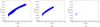 |
Fig. 8. Isosurfaces of Ohmic heating, shaded on a logarithmic scale. Times shown are (a) t = 200, (b) t = 325, and (c) t = 400. The radii of the left, central, and right driving regions are marked on the bottom z = −L plane. |
The nature of the anomalous resistivity imposed confines Ohmic heating, as it does reconnection, to sites where j > jcrit., since Ohmic heating transfers magnetic energy directly to internal energy as a natural consequence of reconnection. The effects being cospatial and similarly caused, magnetic reconnection serves to dissipate accumulated magnetic energy, both through conversion to kinetic energy, and through the associated heating.
In the first time shown, in Fig. 8a, it is clear that there is intense heating arising in association with the large-scale, helical current sheet that emerges as part of the kink instability. This heating is greatest at the original event that triggers reconnection and excites the MHD avalanche. In the second time shown, t = 325 in Fig. 8b, a similar process is under way in the third thread, with the most intense concentration in large-scale helical features in the left-hand thread. Driving being slower in that thread, less magnetic energy has built up, and the heating is weaker. Nonetheless, it concentrates in a similar, crescent-shaped current sheet. At both of these times, there is a multitude of wide-spread, weak, small-scale Ohmic heating events. These mirror the locations of the broad distribution of reconnection sites. By t = 400, Fig. 8c, only highly fragmented, broadly dispersed Ohmic heating events remain, unsurprisingly as this mirrors the reconnection behaviour.
After the progress of the instability, development of reconnection, and repeated disruptions via the avalanche process have destroyed the previous order and structure inherent in the driving, Ohmic heating appears in Fig. 8c as highly fragmented, broadly dispersed, and generally weaker. This has been seen in the general heating (Paper I), but most acutely so for Ohmic heating, whose form emphasizes the disordered spread of currents, magnetic reconnection, and heating.
The spatially analysed Ohmic heating demonstrates precisely the same effect as previously remarked in the volume-integrated instantaneous heating: a few large events clearly proceeding from the original kink and initial disruption of each outer thread, followed by a continuing series of lesser events. There is a notable structural similarity between Figs. 3 and 8, which is expected as Ohmic heating and reconnection occur under the identical condition j > jcrit.. However, since Ohmic heating scales with j2, but the parallel electric field with j∥, the magnitudes of these two properties vary.
In order to compare further Ohmic heating and reconnection as identified by the contours of the field-line-integrated parallel electric field, displayed in Fig. 1, the field-line-integrated Ohmic heating, similarly determined, is shown in Fig. 9 at the selected times used above. A broad similarity is apparent between these graphs and those at the same times in Fig. 1. In particular, at t = 200, in Fig. 8a, the Ohmic heating demonstrates a clear concentration and greatest intensity around the location, to the right of the central thread, where the current sheet associated with the kink instability intersects the mid plane. By the second time, t = 325, Fig. 9b very strong heating is evident around the reconnection event sited approximately at (−1.5,−0.9). The integrated electric field and integrated Ohmic heating have a similar widely dispersed, highly fragmented, and less intense nature at the final time (Fig. 9c). The field-line-integrated electric field and joule heating demonstrate a similarly dispersed, highly fragmented, and less intense nature at the final time, neither showing any evidence of the thread-like structures seen earlier.
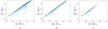 |
Fig. 9. Contours of Ohmic heating integrated along field lines traced from the mid-plane, shaded on a logarithmic scale. Times shown are (a) t = 200, (b) t = 325, and (c) t = 400. |
In a scatter plot of |E∥| values against Ohmic heating (Fig. 10), the fairly good, but imperfect, correlation between these parameters is apparent. The strength of the correlation illustrates that the current is dominated by the component parallel to the magnetic field.
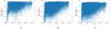 |
Fig. 10. Scatter plots of |E∥| against Ohmic heating at grid points throughout the domain, at times (a) t = 200, (b) t = 325, and (c) t = 400. The red line is an upper bound on E∥ given the value of Ohmic heating and assuming current wholly parallel, i.e. |


Since resistivity is locally determined, and integrating along field lines removes spatial information, one may expect the same quantities, when field-line-integrated, to be slightly less correlated. However, the evident correlation is, in fact, more pronounced. Scatter plots of the field-line-integrated parallel electric field against the field-line-integrated Ohmic heating (Fig. 11) show this correlation, even closer than that of the variables before integration. Except for a few of points (in all cases, fewer than 5% deviate from a best-fitting slope by more than 5%), these integrated terms show almost perfect linearity on the logarithmic scatter plot, which indicates that these parameters scale approximately as:
![$$ \begin{aligned} \int {E_{\parallel }\,\mathrm{d} s} \propto \left[\int {\frac{1}{\sigma }j^2\,\mathrm{d} s}\right]^{\alpha }, \end{aligned} $$](/articles/aa/full_html/2020/01/aa36832-19/aa36832-19-eq27.gif)
where the value of α is determined by finding best-fitting slopes between the two quantities. At t = 200, when reconnection is concentrated in a large-scale, helical current structure, α = 0.95; however, later, when there are far more small-scale reconnection events α = 0.99.
The fact that the index is always α ≈ 1.0 is consistent with a material physical determinant of the values of ∫ E∥ ds and  being the length of the field line along which resistivity is non-zero, which is common between the two. This again highlights the increasing dominance of the parallel component of current.
5.4. Comparison of indicators: correlation
Since we have the full MHD data and are thus in a position so to do, we used the squashing factor Q, the parallel current, and Ohmic heating, to make inferences about the locations of reconnection. A quantitative comparison can be made with the actual sites of reconnection, identified by a non-zero parallel electric field. A coefficient of correlation is determined between ∫ E∥ ds and Q, ∫ j∥ ds, and Ohmic heating on the grid in the mid-plane, and between the local parallel electric field, E∥, and local instantaneous Ohmic heating, throughout the entire three-dimensional volume. This quantitative comparison serves as a one-number summary of the scatter plots given in the previous subsections.
First, the Pearson coefficient is calculated. It is apt to measure the presence of a linear correlation between two data sets. For the pairs of indicators, the Pearson coefficient is set out in Table 1. Mindful that there may be a non-linear trend, the Kendall rank correlation coefficient is calculated. This sacrifices information about the precise value of the properties explored, in this case the indicators, and focuses on the correlation of their rank. The resultant value, bounded between −1 and 1, quantifies the degree to which a monotonic trend exists between two quantities. The comparison is presented in Table 2.
Correlation of reconnection with potential indicators: Pearson coefficient.
Correlation of reconnection with potential indicators: Kendall rank coefficient.
A parallel current may prevail even where there is no reconnection (i.e. where the critical threshold of the magnitude of current is not exceeded). For this reason, it is unsurprising that the parallel current, integrated on field lines, is again less strongly correlated with reconnection. In each of the times considered, Q has a similar level of correlation with reconnection. It appears that this geometric measure of the magnetic field, not accounting for the resistivity and for the definitive electric field, is less apt to indicate the presence of reconnection, since reconnection does not rely solely upon the magnetic field, but is dependent on, for example, the velocity flows involved.
On the other hand, there is notably a much greater correlation between the field-line-integrated parallel current, ∫ j∥ ds, and Q. It is clear from Table 1 that there is a lack of evidence for linearity between them, yet the presence of a less specific form of positive correlation is apparent in the Kendall coefficient from Table 2. Associated scatter plots, in Fig. 12, emphasize this result.
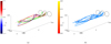 |
Fig. 11. Scatter plots of ∫ E∥ ds against |

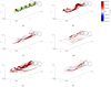 |
Fig. 12. Scatter plots of ∫ j∥ ds against Q at (a) t = 200, (b) t = 325, and (c) t = 400. Both the horizontal and vertical axes are logarithmic. |
6. Conclusions
A three-dimensional numerical simulation of an ideal MHD instability and the ensuing heating in a multi-threaded coronal loop has been analysed. The onset and spatial location of magnetic reconnection following the commencement of an avalanche process, triggered by a kink instability, have been determined. Reconnection, initially heavily concentrated in regions prescribed by the driving velocity, adopts, as the instability proceeds and destroys the initial structure and order, a highly dispersed and sporadic distribution of currents and flows. In a three-dimensional field, it is not straightforward to predict the location of reconnection, in contrast with two-dimensional models, in which reconnection takes place at X-type null points. A localized enhancement of the parallel electric field is a defining indicator of a site of magnetic reconnection.
The location of parallel current, which is connected with the defining marker of reconnection, E∥, shows, not unexpectedly, some correlation with sites of reconnection, as well as having a form, at early times, closely determined by the boundary motions. The Ohmic heating, instigated in common with the occurrence of reconnection, is similarly distributed, and likewise evolves from the initial monolithic arrangement to a highly localized one.
This illustrates clearly the necessarily local and confined nature of the reconnection. Nonetheless, it is noteworthy that such a chaotic and dispersed distribution of reconnection sites proceeds from the action of a large-scale driver with a very simple spatial structure on an originally uniform magnetic field. Strong evidence emerges of a cascade to smaller scales in the magnetic and electric fields. In this respect, we find agreement with the breadth of evidence that reconnection yields fine-scale structure.
The quasi-squashing factor, Q, has been considered as a commonly used predictor for the likely locations of magnetic reconnection. Certainly, Démoulin (2006), for example, observe that evolution under particular forms of shearing can give an approximate relation between maximum current and Q. However, whether there be a quantitative, statistical correlation between Q and the parallel electric field, and whether Q be a good indicator in compressible, turbulent fields, have not been tested previously. We find that, although it offers some suggestion of the appearance of reconnection, the two are less thoroughly matched in the situation at hand, of braided magnetic fields with a large guide field component than, for example, in fields produced by submerged sources (e.g. Maclean et al. 2009) or including topological nulls, an especially material distinction in some parts of the corona. In particular, it appears for our case less pertinent for changes in magnetic topology than other measures, such as Ohmic heating, and than past work has documented albeit in very different contexts, as, for instance, De Moortel & Galsgaard (2006a,b) and Galsgaard et al. (2003). The concept of Q appears a good indicator of likely sites of reconnection within fields having null points, in which topological structures are associated with narrow regions of high Q. Whether these do, in fact, host reconnection is dependent upon the driving velocity field. By lack of null points and a more complex, fragmented distribution of Q, our model differs from those elsewhere studied. Additionally, our model contains flows driving reconnection that are, largely, self-generated by the evolving field: only during the very early evolution does external driving control reconnection. It remains to be determined in which precise regimes and under which conditions Q may be taken reliably to predict regions of reconnecting field lines.
With specific regard to our model, distinct from several others previously evaluated, we argue that Q, being exclusively a measure of the configuration of the magnetic field, does not reflect the electric field or flows of plasma on which reconnection depends. Converging flows may produce reconnection in even relatively smooth fields; the avalanche model gives a good example in the fusion of threads. Regions of high Q denote greatly divergent field lines, which may indeed be the hallmark of a current sheet, but could equally arise from such topological fixtures as null points or separators, which can occur even in a potential field. High Q (indeed, separators with Q → ∞) may arise in potential, current-free fields. Velocity has an important role: current, which facilitates reconnection, has been associated with stagnation flows (Longcope & Strauss 1994). Boundary motions creating such flows have been linked with current sheets at reconnection sites, although the strict need for these motions is queried (Galsgaard et al. 2003; Démoulin 2006). Therefore, high-Q regions are not, by their mere existence, evidence of reconnection, although certainly indicative of the subsequent possibility: and the two, of course, can be coincident, as is documented.
The Ohmic heating is clearly correlated to a material degree with reconnection. We have sought to determine a quantitative relationship, and, in the field-line-integrated results, have found a fairly consistent power law. Consideration remains to be given to the question of which physical factors influence this index, and whether these may cause it to vary among reconnection regimes.
Acknowledgments
JR acknowledges the support of the Carnegie Trust for the Universities of Scotland. AWH and CEP acknowledge the financial support of the STFC through Consolidated Grant ST/S000402/1 to the University of St Andrews. PKB acknowledges financial support of the STFC through Consolidated Grant ST/P000428/1 to the University of Manchester. The authors are grateful to Dr Benjamin M. Williams for the code used for all tracing of field lines for the purposes of this paper; the code uses an RKF45 scheme, details of which are presented by Williams (2018). The authors are further grateful to Prof. R. Alan Cairns, Prof. Peter J. Cargill, Prof. Peter E. Jupp, Prof. Thomas Neukirch, and Dr Antonia Wilmot-Smith for fruitful discussion and helpful suggestions concerning the manuscript. This work used the DiRAC@Durham facility, managed by the Institute for Computational Cosmology, and the Cambridge Service for Data Driven Discovery (CSD3), part of which is operated by the University of Cambridge Research Computing, on behalf of the STFC DiRAC HPC Facility (www.dirac.ac.uk). The DiRAC@Durham equipment was funded by BEIS capital funding via STFC capital grants ST/P002293/1 and ST/R002371/1; Durham University; STFC operations grant ST/R000832/1; BIS National E-infrastructure capital grant ST/K00042X/1; STFC capital grant ST/K00087X/1; and DiRAC Operations grant ST/K003267/1. The DiRAC component of CSD3 was funded by BEIS capital funding via STFC capital grants ST/P002307/1 and ST/R002452/1 and STFC operations grant ST/R00689X/1. DiRAC is part of the National e-Infrastructure. This work used the NumPy (Oliphant 2006) and Matplotlib (Hunter 2007) Python packages.
References
- Arber, T. D., Longbottom, A. W., Gerrard, C. L., & Milne, A. M. 2001, J. Comput. Phys., 171, 151 [NASA ADS] [CrossRef] [Google Scholar]
- Archontis, V., & Hood, A. W. 2013, ApJ, 769, L21 [NASA ADS] [CrossRef] [Google Scholar]
- Aulanier, G., Pariat, E., & Démoulin, P. 2005, A&A, 444, 961 [NASA ADS] [CrossRef] [EDP Sciences] [Google Scholar]
- Aulanier, G., Pariat, E., Démoulin, P., & DeVore, C. R. 2006, Sol. Phys., 238, 347 [NASA ADS] [CrossRef] [Google Scholar]
- Bateman, G. 1978, MHD Instabilities (Cambridge, MA: MIT Press) [Google Scholar]
- Baumann, G., & Nordlund, Å. 2012, ApJ, 759, L9 [NASA ADS] [CrossRef] [Google Scholar]
- Bingert, S., & Peter, H. 2011, A&A, 530, A112 [NASA ADS] [CrossRef] [EDP Sciences] [Google Scholar]
- Bogdan, T. J., & Low, B. C. 1986, ApJ, 306, 271 [NASA ADS] [CrossRef] [Google Scholar]
- Boozer, A. H. 2019, Phys. Plasmas, 26, 042104 [NASA ADS] [CrossRef] [Google Scholar]
- Browning, P. K., Gerrard, C., Hood, A. W., Kevis, R., & Van der Linden, R. A. M. 2008, A&A, 485, 837 [NASA ADS] [CrossRef] [EDP Sciences] [Google Scholar]
- Cairns, R. A. 1985, Plasma Physics (Glasgow: Blackie) [CrossRef] [Google Scholar]
- Carmichael, H. 1964, in The Physics of Solar Flares, ed. W. M. Hess, National Aeronautics and Space Administration, Science and Technical Information Division, 451 [Google Scholar]
- De Moortel, I., & Galsgaard, K. 2006a, A&A, 451, 1101 [NASA ADS] [CrossRef] [EDP Sciences] [Google Scholar]
- De Moortel, I., & Galsgaard, K. 2006b, A&A, 459, 627 [NASA ADS] [CrossRef] [EDP Sciences] [Google Scholar]
- Démoulin, P. 2006, Adv. Space Res., 37, 1269 [NASA ADS] [CrossRef] [Google Scholar]
- Démoulin, P. 2007, AdSpR, 39, 1367 [Google Scholar]
- Démoulin, P., & Priest, E. R. 1997, Sol. Phys., 175, 123 [NASA ADS] [CrossRef] [Google Scholar]
- Démoulin, P., Priest, E. R., & Lonie, D. P. 1996a, J. Geophys. Res., 101, 7631 [NASA ADS] [CrossRef] [Google Scholar]
- Démoulin, P., Henoux, J. C., Priest, E. R., & Mandrini, C. H. 1996b, A&A, 308, 643 [NASA ADS] [Google Scholar]
- Démoulin, P., Bagala, L. G., Mandrini, C. H., Henoux, J. C., & Rovira, M. G. 1997, A&A, 325, 305 [NASA ADS] [Google Scholar]
- Dungey, J. W. 1961, Phys. Rev. Lett., 6, 47 [NASA ADS] [CrossRef] [Google Scholar]
- Galsgaard, K., & Nordlund, Å. 1996, J. Geophys. Res., 101, 13445 [NASA ADS] [CrossRef] [Google Scholar]
- Galsgaard, K., Titov, V. S., & Neukirch, T. 2003, ApJ, 595, 506 [NASA ADS] [CrossRef] [Google Scholar]
- Gekelman, W., Lawrence, E., Collette, A., et al. 2010, Phys. Scr., T142, 014032 [NASA ADS] [CrossRef] [Google Scholar]
- Gekelman, W., Lawrence, E., & Van Compernolle, B. 2012, ApJ, 753, 131 [NASA ADS] [CrossRef] [Google Scholar]
- Gekelman, W., DeHaas, T., Van Compernolle, B., et al. 2016, Phys. Scr., 91, 054002 [NASA ADS] [CrossRef] [Google Scholar]
- Haynes, A. L. 2008, PhD Thesis, University of St Andrews [Google Scholar]
- Haynes, A. L., Parnell, C. E., Galsgaard, K., & Priest, E. R. 2007, Proc. R. Soc. London Ser. A, 463, 1097 [NASA ADS] [CrossRef] [Google Scholar]
- Hesse, M., & Schindler, K. 1988, J. Geophys. Res., 93, 5559 [NASA ADS] [CrossRef] [Google Scholar]
- Hones, Jr., E. W. 1979, Space Sci. Rev., 23, 393 [NASA ADS] [CrossRef] [Google Scholar]
- Hood, A. W., Browning, P. K., & Van der Linden, R. A. M. 2009, A&A, 506, 913 [NASA ADS] [CrossRef] [EDP Sciences] [Google Scholar]
- Hood, A. W., Cargill, P. J., Browning, P. K., & Tam, K. V. 2016, ApJ, 817, 5 [NASA ADS] [CrossRef] [Google Scholar]
- Hood, A. W., & Priest, E. R. 1979, Sol. Phys., 64, 303 [NASA ADS] [CrossRef] [Google Scholar]
- Hunter, J. D. 2007, Comput. Sci. Eng., 9, 90 [NASA ADS] [CrossRef] [Google Scholar]
- Janvier, M. 2017, J. Plasma Phys., 83, 535830101 [Google Scholar]
- Longcope, D. W., & Strauss, H. R. 1994, ApJ, 437, 851 [NASA ADS] [CrossRef] [Google Scholar]
- Low, B. C. 1985, ApJ, 293, 31 [NASA ADS] [CrossRef] [Google Scholar]
- Maclean, R. C., Büchner, J., & Priest, E. R. 2009, A&A, 501, 321 [NASA ADS] [CrossRef] [EDP Sciences] [Google Scholar]
- Mandrini, C. H., Demoulin, P., Schmieder, B., et al. 2006, Sol. Phys., 238, 293 [NASA ADS] [CrossRef] [Google Scholar]
- Masson, S., Pariat, E., Aulanier, G., & Schrijver, C. J. 2009, ApJ, 700, 559 [NASA ADS] [CrossRef] [Google Scholar]
- McClements, K. G. 2019, AdSpR, 63, 1443 [NASA ADS] [Google Scholar]
- Milano, L. J., Dmitruk, P., Mandrini, C. H., Gómez, D. O., & Démoulin, P. 1999, ApJ, 521, 889 [NASA ADS] [CrossRef] [Google Scholar]
- Neukirch, T. 1995, A&A, 301, 628 [NASA ADS] [Google Scholar]
- Oliphant, T. E. 2006, A Guide to NumPy (USA: Trelgol Publishing) [Google Scholar]
- Pariat, E., & Démoulin, P. 2012, A&A, 541, A78 [NASA ADS] [CrossRef] [EDP Sciences] [Google Scholar]
- Parnell, C. E. 2018, in Electric Currents in Geospace and Beyond, eds. A. Keiling, O. Marghitu, & M. Wheatland, Washington DC Am. Geophys. Union Geophys. Monograph Ser., 235, 219 [NASA ADS] [CrossRef] [Google Scholar]
- Parnell, C. E., & Galsgaard, K. 2004, A&A, 428, 595 [NASA ADS] [CrossRef] [EDP Sciences] [Google Scholar]
- Parnell, C. E., Maclean, R. C., & Haynes, A. L. 2010, ApJ, 725, L214 [NASA ADS] [CrossRef] [Google Scholar]
- Phan, T. D., Eastwood, J. P., Cassak, P. A., et al. 2016, Geophys. Res. Lett., 43, 6060 [NASA ADS] [CrossRef] [Google Scholar]
- Pontin, D. I. 2012, Phil. Trans. R. Soc. Ser. A, 370, 3169 [Google Scholar]
- Priest, E., & Forbes, T. 2000, Magnetic Reconnection: MHD Theory and Applications (Cambridge: Cambridge University Press) [CrossRef] [Google Scholar]
- Priest, E. R., & Démoulin, P. 1995, J. Geophys. Res., 100, 23443 [NASA ADS] [CrossRef] [Google Scholar]
- Raouafi, N. E., Patsourakos, S., Pariat, E., et al. 2016, Space Sci. Rev., 201, 1 [NASA ADS] [CrossRef] [Google Scholar]
- Reid, H. A. S., Vilmer, N., Aulanier, G., & Pariat, E. 2012, A&A, 547, A52 [NASA ADS] [CrossRef] [EDP Sciences] [Google Scholar]
- Reid, J., Hood, A. W., Parnell, C. E., Browning, P. K., & Cargill, P. J. 2018, A&A, 615, A84 [NASA ADS] [CrossRef] [EDP Sciences] [Google Scholar]
- Restante, A. L. 2011, PhD Thesis, University of St Andrews [Google Scholar]
- Ross, J., & Latter, H. N. 2018, MNRAS, 477, 3329 [NASA ADS] [CrossRef] [Google Scholar]
- Schindler, K., Hesse, M., & Birn, J. 1988, J. Geophys. Res., 93, 5547 [NASA ADS] [CrossRef] [Google Scholar]
- Stanier, A., Browning, P., Gordovskyy, M., et al. 2013, Phys. Plasmas, 20, 122302 [NASA ADS] [CrossRef] [Google Scholar]
- Sturrock, P. A. 1966, Nature, 211, 695 [NASA ADS] [CrossRef] [Google Scholar]
- Tam, K. V., Hood, A. W., Browning, P. K., & Cargill, P. J. 2015, A&A, 580, A122 [NASA ADS] [CrossRef] [EDP Sciences] [Google Scholar]
- Tassev, S., & Savcheva, A. 2017, ApJ, 840, 89 [NASA ADS] [CrossRef] [Google Scholar]
- Titov, V. S. 2007, ApJ, 660, 863 [NASA ADS] [CrossRef] [Google Scholar]
- Titov, V. S., Galsgaard, K., & Neukirch, T. 2003, ApJ, 582, 1172 [NASA ADS] [CrossRef] [Google Scholar]
- Titov, V. S., Hornig, G., & Démoulin, P. 2002, J. Geophys. Res., 107, 1164 [Google Scholar]
- Vasyliunas, V. M. 1984, in Magnetic Reconnection in Space and Laboratory Plasmas, ed. E. W. Hones, Jr., 25 [NASA ADS] [CrossRef] [Google Scholar]
- Wendel, D. E., Olson, D. K., Hesse, M., Karimabadi, H., & Daughton, W. S. 2013, AGU Fall Meeting Abstracts, SM13A [Google Scholar]
- Williams, B. M. 2018, PhD Thesis, University of St Andrews [Google Scholar]
- Wilmot-Smith, A. L., Hornig, G., & Pontin, D. I. 2009, ApJ, 704, 1288 [NASA ADS] [CrossRef] [Google Scholar]
- Wilmot-Smith, A. L., Pontin, D. I., & Hornig, G. 2010, A&A, 516, A5 [NASA ADS] [CrossRef] [EDP Sciences] [Google Scholar]
- Wright, A. N. 1987, Planet. Space Sci., 35, 813 [NASA ADS] [CrossRef] [Google Scholar]
- Wyper, P. F., & Pontin, D. I. 2014, Phys. Plasmas, 21, 102102 [NASA ADS] [CrossRef] [Google Scholar]
- Yamada, M. 2010, Am. Astron. Soc. Meet. Abstr., 216, 209.02 [NASA ADS] [Google Scholar]
- Zweibel, E. G., & Yamada, M. 2016, Proc. R. Soc. London Ser. A, 472, 20160479 [NASA ADS] [CrossRef] [Google Scholar]
All Tables
Correlation of reconnection with potential indicators: Kendall rank coefficient.
All Figures
|
Fig. 1. Contours of the field-line-integrated parallel electric field, plotted where field lines intersect the mid-plane. Times shown are (a) t = 175, (b) t = 200, (c) t = 225, (d) t = 275, (e) t = 325, and (f) t = 400. Times (b), (e), and (f) are subsequently considered in greater detail. In (a), the dashed black lines indicate the radii of the driven regions, representing footpoints of the left, central, and right threads. The contours are shaded according to the logarithmic scale on the colour bar. |
| In the text | |
|
Fig. 2. Sample of field lines traced from the mid-plane, coloured (a) solidly according to ∫ E∥ ds and (b) parametrically according to current, |j|(s). Plots are shown at t = 200. In (a), green denotes a field line along which ∫ E∥ ds = 0. In (b), all |j| ≤ jcrit. = 5.0 is shaded blue, and current with magnitude above the critical threshold is shaded according to the colour bar. The radii of the driving regions are marked on the bottom z = −L plane. |
| In the text | |
|
Fig. 3. Isosurfaces of local E∥. Times shown are (a) t = 175, (b) t = 200, (c) t = 225, (d) t = 275, (e) t = 325, and (f) t = 400. On (a) is superimposed a sample of field lines in green. The radii of the left, central, and right driving regions are marked on the bottom z = −L plane. Times (b), (e), and (f) are subsequently considered in greater detail. The isosurfaces are shaded according to the logarithmic scale on the colour bar. |
| In the text | |
|
Fig. 4. Quasi-squashing factor Q found in the mid-plane, at (a) t = 200, (b) t = 325, and (c) t = 400. We have taken the maximum of the values with respect to the bottom and top planes. The contours are shaded according to the logarithmic scale on the colour bar. |
| In the text | |
|
Fig. 5. Histograms of values of Q in the mid-plane, at (a) t = 200, (b) t = 325, and (c) t = 400; and scatter plots showing the distribution of values of Q and ∫ E∥ ds at the same point in the mid-plane, at (d) t = 200, (e) t = 325, and (f) t = 400. In order to represent the full distribution on a single set of axes, the histograms are produced with frequency density (the vertical axis) and Q (the horizontal axis) each on a logarithmic scale. The blue bars indicate the distribution where ∫ E∥ ds = 0, and the red that where ∫ E∥ ds ≠ 0. The histograms are normalized such that the two histograms for each time have a combined area of unity. The scatter plots are also produced on a logarithmic scale. |
| In the text | |
|
Fig. 6. Contours of the field-line-integrated parallel electric current in the mid-plane. Times shown are (a) t = 175, (b) t = 200, (c) t = 225, (d) t = 275, (e) t = 325, and (f) t = 400, as in Figs. 1 and 3. |
| In the text | |
|
Fig. 7. Histograms showing the distribution of ∫ j∥ ds where the corresponding field-line-integrated parallel electric field is zero (blue) or non-zero (red) at (a) t = 200, (b) t = 325, and (c) t = 400; and scatter plots of ∫ E∥ ds against ∫ j∥ ds in the mid-plane at (d) t = 200, (e) t = 325, and (f) t = 400. The histograms are normalized such that the two histograms for each time have a combined area of unity. Both histograms and scatter plots are drawn on logarithmic axes. |
| In the text | |
|
Fig. 8. Isosurfaces of Ohmic heating, shaded on a logarithmic scale. Times shown are (a) t = 200, (b) t = 325, and (c) t = 400. The radii of the left, central, and right driving regions are marked on the bottom z = −L plane. |
| In the text | |
|
Fig. 9. Contours of Ohmic heating integrated along field lines traced from the mid-plane, shaded on a logarithmic scale. Times shown are (a) t = 200, (b) t = 325, and (c) t = 400. |
| In the text | |
|
Fig. 10. Scatter plots of |E∥| against Ohmic heating at grid points throughout the domain, at times (a) t = 200, (b) t = 325, and (c) t = 400. The red line is an upper bound on E∥ given the value of Ohmic heating and assuming current wholly parallel, i.e. |
| In the text | |
|
Fig. 11. Scatter plots of ∫ E∥ ds against |
| In the text | |
|
Fig. 12. Scatter plots of ∫ j∥ ds against Q at (a) t = 200, (b) t = 325, and (c) t = 400. Both the horizontal and vertical axes are logarithmic. |
| In the text | |
Current usage metrics show cumulative count of Article Views (full-text article views including HTML views, PDF and ePub downloads, according to the available data) and Abstracts Views on Vision4Press platform.
Data correspond to usage on the plateform after 2015. The current usage metrics is available 48-96 hours after online publication and is updated daily on week days.
Initial download of the metrics may take a while.