| Issue |
A&A
Volume 669, January 2023
|
|
|---|---|---|
| Article Number | A33 | |
| Number of page(s) | 17 | |
| Section | The Sun and the Heliosphere | |
| DOI | https://doi.org/10.1051/0004-6361/202245142 | |
| Published online | 03 January 2023 | |
Comparison of magnetic energy and helicity in coronal jet simulations
1
Sorbonne Université, École polytechnique, Institut Polytechnique de Paris, Université Paris Saclay, Observatoire de Paris-PSL, CNRS, Laboratoire de Physique des Plasmas (LPP), 4 place Jussieu, 75005 Paris, France
e-mail: This email address is being protected from spambots. You need JavaScript enabled to view it.
2
Durham University, Department of Mathematical Sciences, Stockton Road, Durham DH1 3LE, UK
3
Centre for Mathematical Plasma Astrophysics, Departement of Mathematics, KU Leuven, Celestijnenlaan 200 B, 3001 Leuven, Belgium
Received:
5
October
2022
Accepted:
13
November
2022
Abstract
Context. While non-potential (free) magnetic energy is a necessary element of any active phenomenon in the solar corona, its role as a marker of the trigger of the eruptive process remains elusive. Meanwhile, recent analyses of numerical simulations of solar active events have shown that quantities based on relative magnetic helicity could highlight the eruptive nature of solar magnetic systems.
Aims. Based on the unique decomposition of the magnetic field into potential and non-potential components, magnetic energy and helicity can also both be uniquely decomposed into two quantities. Using two 3D magnetohydrodynamics parametric simulations of a configuration that can produce coronal jets, we compare the dynamics of the magnetic energies and of the relative magnetic helicities.
Methods. Both simulations share the same initial setup and line-tied bottom-boundary driving profile. However, they differ by the duration of the forcing. In one simulation, the system is driven sufficiently so that a point of no return is passed and the system induces the generation of a helical jet. The generation of the jet is, however, markedly delayed after the end of the driving phase; a relatively long phase of lower-intensity reconnection takes place before the jet is eventually induced. In the other reference simulation, the system is driven during a shorter time, and no jet is produced.
Results. As expected, we observe that the jet-producing simulation contains a higher value of non-potential energy and non-potential helicity compared to the non-eruptive system. Focussing on the phase between the end of the driving-phase and the jet generation, we note that magnetic energies remain relatively constant, while magnetic helicities have a noticeable evolution. During this post-driving phase, the ratio of the non-potential to total magnetic energy very slightly decreases while the helicity eruptivity index, which is the ratio of the non-potential helicity to the total relative magnetic helicity, significantly increases. The jet is generated when the system is at the highest value of this helicity eruptivity index. This proxy critically decreases during the jet-generation phase. The free energy also decreases but does not present any peak when the jet is being generated.
Conclusions. Our study further strengthens the importance of helicities, and in particular of the helicity eruptivity index, to understand the trigger mechanism of solar eruptive events.
Key words: Sun: magnetic fields / magnetohydrodynamics (MHD) / magnetic reconnection / methods: numerical / Sun: activity
© The Authors 2023
 Open Access article, published by EDP Sciences, under the terms of the Creative Commons Attribution License (https://creativecommons.org/licenses/by/4.0), which permits unrestricted use, distribution, and reproduction in any medium, provided the original work is properly cited.
This article is published in open access under the Subscribe-to-Open model. This email address is being protected from spambots. You need JavaScript enabled to view it. to support open access publication.
1. Introduction
Understanding the physical processes at the origin of active solar events is a central problem of solar physics. Numerous and diverse models for eruptive events have been developed over time that aim to explain the different observational features of solar activity. Over the last few years, an interest in the relation between magnetic helicity and solar eruptivity has been renewed (e.g. reviews of Pevtsov et al. 2014; Toriumi & Park 2022), driven by advances in the theory of helicity measurements (cf. review sections of Démoulin 2007; Démoulin & Pariat 2009; Valori et al. 2016).
Magnetic helicity, ℋm (cf. Eq. (7)), quantifies the level of entanglement of the magnetic field lines in a closed magnetic system. It is a signed quantity, the classical definition of which was initially introduced by Elsasser (1956). Magnetic helicity has the quasi-unique property of being an invariant of ideal magnetohydrodynamics (MHD; Woltjer 1958). The concept was later reviewed by Berger & Field (1984) and Finn & Antonsen (1985), putting the focus on relative magnetic helicity, HV (cf. Eq. (8)), a gauge-invariant quantity that can be used to study non-magnetically closed systems, and hence is more suitable for natural plasmas. Using numerical simulations, Pariat et al. (2015b) confirmed the hypothesis introduced by Taylor (1974) that even in the presence of non-ideal dynamics, the dissipation of relative magnetic helicity is negligible. Relative magnetic helicity cannot be dissipated or created within the corona, and thus can only be transported or annihilated. This conservation property has several major consequences, one of which possibly being that coronal mass ejections (CMEs) are the consequence of the evacuation of an excess of helicity (Rust 1994; Low 1996).
In the last ten years, robust methods have been developed (see review of Valori et al. 2016) that enable the estimation of helicity in finite volumes (e.g. Thalmann et al. 2011; Valori et al. 2012; Moraitis et al. 2018), helicity fluxes (e.g. Dalmasse et al. 2014; Pariat et al. 2015b; Linan et al. 2018; Schuck & Antiochos 2019), and helicity per field line (e.g. Russell et al. 2015; Aly 2018; Yeates & Page 2018; Moraitis et al. 2019a). Thanks to these developments, in recent years, magnetic helicity has constituted a renewed perspective to analyse and understand the generation of solar active events such as jets, flares, and eruptions (e.g. Knizhnik et al. 2015; Zhao et al. 2015; Priest et al. 2016). Different observed solar active regions have recently been investigated for their helicity content and dynamics. (Valori et al. 2013; Moraitis et al. 2014, 2019b; Guo et al. 2017; Polito et al. 2017; Temmer et al. 2017; James et al. 2018; Thalmann et al. 2019b, 2021; Price et al. 2019; Gupta et al. 2021; Green et al. 2022; Lumme et al. 2022).
Similar to magnetic energy, relative magnetic helicity can be decomposed when considering the potential and non-potential part of a magnetic field in a domain. Berger (2003) introduced the decomposition of the relative magnetic helicity into two gauge-invariant components (cf. Eq. (9)) : a non-potential helicity, Hj related to the current carrying magnetic field and a complementary volume-threading helicity, Hpj. Pariat et al. (2017) suggested that the ratio, ηH (cf. Eq. (12)), of the current carrying helicity to the relative helicity could constitute an interesting proxy of when solar-like magnetic systems become eruptive.
From 3D parametric simulations of solar coronal eruption (Zuccarello et al. 2015) driven by distinct line-tied boundary motions, Zuccarello et al. (2018) studied the impact of the different driving flows on the helicity and energy injection. They found that the helicity ratio ηH was clearly associated with the eruption trigger since the different eruptions occurred exactly when the ratio reached the very same threshold value. Pariat et al. (2017) followed and estimated the helicity eruptivity index, ηH, in a set of seven simulations of the formation of solar active regions (Leake et al. 2013, 2014). The different simulations led to either stable or eruptive configurations. Pariat et al. (2017) observed that the helicity ratio was discriminating the two types of dynamics: stable or eruptive. Linan et al. (2018) and Moraitis et al. (2014) also analysed simulations in which the helicity eruptivity index presented a peak for systems leading to eruptive behaviour.
These results motivated Linan et al. (2018) to better understand the properties of Hj and Hpj. Linan et al. (2018) provided the first analytical formulas of the time variation of non-potential and volume-threading helicity. They found that the evolutions of the current-carrying and the volume-threading helicities are partially controlled by a transfer term that reflects the exchange between these two kinds of helicity. This transfer term can even dominate the dynamics of non-potential helicity. The properties of the fluxes of helicities were further studied by Linan et al. (2018), along with the dynamics of the energies. Linan et al. (2020) noted that magnetic helicities provided additional information on the trigger mechanism of the eruptive event comparatively to magnetic energies. Analysing the helicity flux of the simulations of Zuccarello et al. (2015, 2018), they also showed that the threshold in the helicity eruptivity index could be reached by a different evolution of Hj and Hpj, implying that reaching the threshold was more important than the way in which the threshold was reached.
In observations, the analysis of the helicity eruptivity index required the knowledge of the magnetic field in the whole studied domain. As Linan et al. (2018) demonstrated, Hj and Hpj cannot be estimated from their flux through the photosphere, unlike what is frequently done with relative magnetic helicity (e.g. as in Chae 2001; Nindos et al. 2003; Pariat et al. 2005, 2006; Dalmasse et al. 2013, 2014, 2018; Liokati et al. 2022). Estimates of Hj and Hpj must therefore rely on magnetic extrapolation of the coronal field from photospheric measurements (cf. reviews Wiegelmann & Sakurai 2012; Wiegelmann et al. 2014). Such extrapolation must produce fields with a high degree of solenoidality for the helicity estimate to be trustworthy (Thalmann et al. 2019a,b, 2020; Thalmann et al. 2021, 2022). The helicity eruptivity index has been estimated prior to the onset of several active phenomena (James et al. 2018; Moraitis et al. 2019b; Price et al. 2019; Thalmann et al. 2019b, 2021; Gupta et al. 2021; Lumme et al. 2022). These studies have consistently found that high values of the helicity eruptivity index indeed indicate the potential of active regions to produce eruptive events. On the contrary, very low values of the index were found prior to confined (CME-less) GOES X-class flares (Thalmann et al. 2019b; Gupta et al. 2021). Lumme et al. (2022) carried out a data-driven model of build-up of a magnetic field before an eruption in AR NOAA 11726. They showed the formation of a pre-eruptive coronal flux rope, and analysed the evolution of magnetic helicity and dynamics of the helicity eruptivity index. The flux rope constituted only a fraction of the whole active region. They noted that the index steadily increased when considering the whole domain, with no decrease after the eruption. When only taking into account the domain where the eruptive flux rope was located, the helicity eruptivity index displayed peaks before the eruption time. Thoroughly analysing the link between the variations in the helicity index and every form of activity developing in AR NOAA 11158, Green et al. (2022) found the helicity ratio variations to be more pronounced during times of strong flux emergence, collision and reconnection between fields of different bipoles, shearing motions, and reconfiguration of the corona through failed and successful eruptions. It was observed to a high degree that any form of eruptivity (jets, failed eruptions, eruptions) had a signature in the helicity eruptivity index. Even jets developing at a smaller scale than the whole active region, over which the helicity eruptivity index was calculated, were related with fluctuations of the index.
The abovementioned findings motivated the present study to analyse the properties of helicities in coronal jet simulations, and the link between the generation of such activity with the helicity eruptivity index. In the present study, we perform a new innovative analysis of the parametric 3D MHD simulations of Wyper et al. (2018) to investigate the time variations of magnetic energies and magnetic helicities. We analyse two simulations with a very similar setup, one inducing a jet and one without eruptive activity. In both simulations helicity and energy are injected thanks to line-tied boundary forcing, although for a slightly longer time in the simulation in which a jet is induced. However, the jet is not induced immediately after the forcing, but rather after a delayed period in which a reconfiguration of the magnetic system is observed. A period of less substantial reconfiguration is also noted in the stable configuration. In the present work, we aim to compare the dynamics, in terms of energies and helicities, of this post-driving (reconfiguration) phase in the jet-producing versus the non-eruptive case. We also examine whether the transfer term between the two helicity components, Hj and Hpj, plays a major role in the helicity budgets, as was observed in (Linan et al. 2018). Finally, we want to see if the helicity eruptive index is able to discriminate the two simulations, the eruptive from the non-eruptive one, and if it is able to provide sensible information about the eruptivity of the magnetic system.
Our manuscript is decomposed into different sections, organised as follows. In Sect. 2, we first summarise the concept and properties of the numerical experiments of Wyper et al. (2018) that are analysed in the present study. In Sect. 3, we then introduce the methods employed to estimate magnetic energy and helicity, and their decomposition based on potential and non-potential magnetic field, as well as the helicity fluxes. The analysis of the dynamics of energies and helicities in the two simulations is presented in Sect. 4. Finally, in Sect. 5, we summarise our results and discuss them in the broader context of the problem of the trigger of active solar events.
2. Non-eruptive and jet-producing numerical simulations
2.1. Numerical model
Motivated by a growing number of jet observations revealing minifilament and sigmoid eruptions (e.g. Raouafi et al. 2010; Sterling et al. 2015), the jet simulations of Wyper et al. (2017, 2018) were designed to explore the nature of filament channel eruptions in coronal jets and how they compare to large-scale CME-producing active region eruptions. The key feature of the model is that the initial magnetic field is comprised of a 3D magnetic null-point topology above a bipolar surface flux distribution, which is surrounded by uniform vertical (or tilted) open field. Line-tied surface motions lead to the formation of a filament channel at the centre of the bipole while maintaining the same surface flux distribution (Pariat et al. 2009). As outlined below, subject to sufficient forcing, the filament channel becomes destabilised and erupts. This destabilisation is aided entirely, or in-part, by null-point reconnection above the filament channel, which, as shown in Wyper et al. (2017), is exactly analogous to the ‘breakout reconnection’ hypothesis generating active region CMEs (Antiochos et al. 1999). Kumar et al. (2018, 2019), amongst others, have shown that this model captures many observational features of coronal jets. This realism, along with the involvement of a flux rope in the eruption, makes this model an ideal test for the helicity index.
Here we focus on the simulation from Wyper et al. (2018) with a vertical open field and consider two cases. The jet-producing simulation described in Wyper et al. (2018), in which the driving was ramped up to a constant speed over a period of 50 non-dimensional time units, held constant until t = 300 and then ramped down to zero (again over 50 time units). And a new non-eruptive case, similar to the first but where the driving was held constant instead until t = 250 before being ramped down. Both simulations were identical, except the grid was allowed to adaptively refine one further level for the jet-producing case to better delineate the different phases of the eruptive evolution. However, as outlined below, their early evolution prior to t = 250 was quasi-identical. In both, the ideal compressible MHD equations were solved using the ARMS code (DeVore & Antiochos 2008), with reconnection occurring due to diffusion intrinsic to the numerical scheme. For context, one time unit is roughly the Alfvén travel time across the width of the separatrix dome based on the maximal Alfvén speed on the surface.
2.2. Common initial forcing phase
The left panels of Fig. 1 show representative field lines and the current density in the two simulations at t = 0 and at the end of the common driving phase (t = 250). The cyan field lines connect the two halves of the surface bipolar patch. At t = 250 these field lines form part of the strapping field above the filament channel formed by the action of the driving (yellow field lines). At the end of this common forcing phase, the simulations are near identical. Only slight differences in the field line morphology within the filament channel are present by the end of this phase due to the differences in local resolution, with the better resolved jet case containing sheared field lines that extend slightly further along the polarity inversion line (PIL).
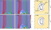 |
Fig. 1. Snapshots of the common initial phase (0 < t < 250) of both simulations. Left panels: electric current density distribution in a central 2D cut and magnetic field lines. Right: QSL distribution at t = 250. The dashed line shows the PIL. Top panels: non-eruptive case. Bottom panels: jet-producing case. Yellow shading indicates the open field. |
The right panels of Fig. 1 show the squashing factor, Q, on the surface (Titov et al. 2002; Titov 2007; Pariat & Démoulin 2012), with the yellow shaded region indicating the open field. The squashing factor is related to the gradients of the magnetic connectivity of the field lines. Volumes of high Q, named quasi-separatrix layers (QSLs, Démoulin et al. 1996; Longcope 2005) delimit (quasi-)connectivity domains and represent preferential sites for the build-up of electric currents (Aulanier et al. 2005, 2006). A true separatrice is always embedded in a QSL halo (Pontin et al. 2016), and hence the Q distribution also captures the location of the fan and the spine of a 3D null point (Masson et al. 2009, 2017).
Here, both distributions of Q are very similar, with the circular footprint of the fan separatrix and QSL around the inner spine in close agreement. Parallel strips of high Q flank the right side of the PIL (the centre of the surface bipole flux distribution), indicating that a small flux rope has formed as a result of gradients in the surface driving profile. This filament channel flux rope wraps around the polarity inversion line with foot points as indicated. One starts to observed, in particular for the inner flux rope footpoint, the characteristic hook shape in the distribution of Q associated with flux rope (Zhao et al. 2016).
2.3. Non-eruptive simulation
Beyond t = 250 the driving in the non-eruptive case ramps down to zero. This phase is named the post-driving phase of the non-eruptive simulations. The injected shear sufficiently expands the closed field so that the null point is stressed and low-intensity reconnection is induced. Figure 2 shows the field lines and QSLs not long after the driving is halted and at a substantial time later (t = 800). The low-intensity reconnection has closed down some of the red open field lines while simultaneously opening up some of the strapping field (Fig. 2, top right panel). This can also be seen in the leftward shift of the footprint of the fan separatrix (Fig. 2, bottom right panel). By t = 800 this low-intensity reconnection has dissipated the stress around the null point and the reconnection effectively ceases, while the filament channel remains stable. The system remains almost unchanging from then on.
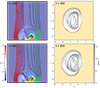 |
Fig. 2. Snapshots at t = 350 and 800, for the non-eruptive simulation. Left panels: electric current density and field lines. Right panels: QSL distribution. Yellow shading indicates the open field. |
2.4. Jet-producing simulation
By contrast, in the jet-producing simulation, the longer driving time tips the system into an unstable regime. This implies a point of no return is passed between when the driving is halted at t = 300 versus t = 350. In this case, after t = 350, the system enters a long phase of sustained null-point reconnection, denoted as the ‘breakout phase’ in Wyper et al. (2018), following a feedback between the upward expansion of the flux rope and the removal of strapping field above it (Fig. 3, top left panels). At the same time reconnection also occurs at the current layer beneath the flux rope. The result is that the strapping cyan field lines are steadily removed from above the flux rope, while the flux rope itself both lengthens and increases in overall magnetic flux (compare the left panels at t = 350 and 700). That is to say during this phase a larger fraction of the closed field magnetic flux becomes part of a single, coherent flux rope, while simultaneously the strapping field linking with it is removed. The removal of strapping field is discernible in the squashing degree (Q) plot at t = 700 by the leftward shift of the fan separatrix, while the broader area spanned by the QSL hooks indicates the increase in the magnetic flux contained within the flux rope. It should be noted that although the reconnection in both current sheets is sustained, it is not explosive or impulsive during this phase and the flux rope rises slowly. In this study, this phase, between t = 350 and t ∼ 740, is labelled the post-driving phase of the jet-producing simulation.
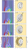 |
Fig. 3. Snapshots at t = 350, 700, 760, and 850 for the jet-producing simulation. Left panels: electric current density and field lines. Right panels: QSL distribution. Yellow shading indicates the open field. |
As more fully discussed in Wyper et al. (2018), an impulsive change in the evolution occurs when the strapping field is exhausted and the flux rope encounters the null point current sheet. This occurs around t = 740, after which the flux rope rapidly begins to reconnect with the open field, transferring a faction of the twist within the flux rope to the open field. This is shown in the QSL plot at t = 760 by one foot point of the flux rope partly now residing in the open field region, while at t = 850 (once the jet is launched) the rest of the sheared closed field has now also become open. This transfer of twist, in addition to the reconnection outflows, is what forms the jet (cf. Shibata & Uchida 1986; Pariat et al. 2009, 2015a, 2016; Wyper et al. 2017, 2018). This period is named the jet onset phase.
3. Estimation methods of magnetic energies and helicities
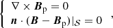
In the following section, we introduce the method used to numerically compute the magnetic energies and helicities in the two simulations, as well as some derived quantities such as helicity fluxes and the helicity eruptivity index, ηH. Our analyses primarily relies on the determination of the unique potential field Bp of B, which has the same flux distribution of B through the boundary 𝒮 of the domain 𝒱 and satisfies:
 (1)
(1)
where n is the outward-pointing unit vector locally normal to 𝒮. The potential field, Bp, can thus be defined through the use of the scalar function, ϕ, which is the solution of the Laplace equation with Neumann boundary conditions:
 (2)
(2)
For a given magnetic field, B, studied in a simply connected domain, the potential field Bp is uniquely defined. The magnetic field B is thus uniquely decomposed as:
 (3)
(3)
with Bj being the non-potential field, uniquely defined as the difference Bj = B − Bp. The field Bj is the current-carrying part of the field since ∇ × B = ∇ × Bj = μ0j, following the Ampère–Maxwell law, with j being the electric current density and μ0 the magnetic constant.
3.1. Magnetic energy decomposition
Using the decomposition of B into current-carrying and potential components (cf. Eq. (3)), for a strictly solenoidal field (∇ ⋅ B = 0), the total magnetic energy Etot can be classically decomposed as (Thompson’s theorem):
 (4)
(4)
where Epot is the potential energy and Efree is the energy of the non-potential field, frequently also called the free magnetic energy.
When B is not strictly solenoidal, for example when B is represented over a discrete mesh, such as in numerical experiments, Valori et al. (2013) have shown that the energy of the magnetic field in 𝒱 can be distributed into solenoidal and non-solenoidal contributions, as in:
 (5)
(5)
where Epot and Efree are the energies associated with the potential and current-carrying solenoidal contributions, Epot,ns and Efree,ns are those of the non-solenoidal contributions, and Emix is a non-solenoidal mixed term (see Eqs. (7), (8) in Valori et al. 2013, for the corresponding expressions). All terms in Eq. (5) are positively defined, except for Emix. For a perfectly solenoidal field, Epot,ns = Efree,ns = Emix = 0, which recovers the Thomson’s theorem.
Following Valori et al. (2016), to analyse the eventual impact of the non-solenoidality in the discretised data, we considered a single number for characterising the energy associated with the non-solenoidal components of the field, given by:
 (6)
(6)
This method, which has now been regularly used (Valori et al. 2016; Pariat et al. 2017; Moraitis et al. 2019b; Thalmann et al. 2019a,b, 2021), is basically a numerical verification of Thomson’s theorem, and allows one to quantify the effect of a (numerical) finite divergence of the magnetic field in terms of associated energies. The derived values of Ediv in both simulations are extremely small and only correspond to about 0.1 − 0.2% of Etot. These values can be compared to the different test cases of Valori et al. (2013), with similar amplitudes to the analytical test over a discrete grid. The simulations are thus highly solenoideal. For these values of Ediv/Etot, magnetic helicity estimations are extremely reliable (cf. Sect. 7 of Valori et al. 2016).
3.2. Relative magnetic helicity decomposition
In the fixed volume 𝒱 bounded by the surface 𝒮, the magnetic helicity, ℋm, is classically defined as:
 (7)
(7)
where A is the vector potential of the studied magnetic field B, that is to say, ∇ × A = B. In practice, this scalar description of the geometrical properties of magnetic field lines is relevant only if the magnetic field is tangential to the surface (i.e. if V is a magnetically bounded volume). Indeed, the magnetic helicity is gauge invariant if, and only if, this condition is respected. For the study of natural plasmas, especially in solar physics, the magnetic field does not satisfy this condition, the solar photosphere being subject to significant flux.
In order to lift this caveat, Berger & Field (1984) introduced the concept of relative magnetic helicity, a gauge-invariant quantity, based on a reference field. Using Ap, the vector potential of the potential field, Bp = ∇ × Ap, the relative magnetic helicity provided by Finn & Antonsen (1985) is:
 (8)
(8)
In this form, the relative magnetic helicity is gauge invariant for both Ap and A. The difference between the potential field and the magnetic field can be written as a non-potential magnetic field, Bj = B − Bp, associated with the vector Aj, defined as Aj = A − Ap, such that ∇×Aj = Bj. Following Berger (2003), HV can be divided into two gauge-invariant quantities (see also Pariat et al. 2017; Linan et al. 2018, 2020):
 (9)
(9)
 (10)
(10)
 (11)
(11)
where Hj is the non-potential magnetic helicity associated with the current-carrying component of the magnetic field, Bj, and Hpj is the volume-threading helicity involving both B and Bp. By construction, both Hj and Hpj are gauge invariant, since Bj has no normal contribution to the surface 𝒮.
3.3. Helicity eruptivity index
Following Pariat et al. (2017), we define the helicity eruptivity index, ηH, as the ratio of the non-potential helicity to the total relative helicity:
 (12)
(12)
This non-dimensional ratio is defined positively here. It should be noted that since helicities are signed quantities, Hj and HV can have opposite signs. The index ηH is also not bounded by 1 since Hj can exceed HV. This may happen in the case where Hpj and Hj have opposite signs, as in the jet case analysed by Linan et al. (2018). In the present simulations, however, all helicities are positive and one thus has: ηH = Hj/HV.
We note that Yang et al. (2020) have proposed an alternative definition of the helicity eruptivity index, based on a periodic potential field. This index may be more suited for systems with a higher degree of periodicity, very distinct from the one studied here.
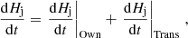
3.4. Hj and Hpj time variations
The study of the time variations of relative magnetic helicity has now benefited from two decades of investigations (e.g. Chae 2001, 2007; Pariat et al. 2005, 2015b; Dalmasse et al. 2014; Schuck & Antiochos 2019). Relative magnetic helicity being a conserved quantity in ideal MHD, its time variations can be solely written as the results of a flux through the boundary of the studied domain (cf. Sect. 2 of Pariat et al. 2015b). In ideal MHD, there is no volume term that would dissipate or create magnetic helicity. Additionally, the time variations of HV,dHV/dt , can trivially be related to the time variations dHj/dt and dHpj/dt of Hj and Hpj respectively:
 (13)
(13)
Motivated by the interest to understand the properties of Hj and Hpj, Linan et al. (2018) have studied the time variation of these helicities. Linan et al. (2018) have established the following gauge-invariant equations of the evolution equations of dHj/dt and dHpj/dt:
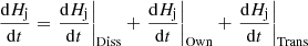 (14)
(14)
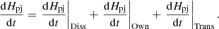 (15)
(15)
The terms dHj/dt|Diss and dHpj/dt|Diss (whose formulations can be obtain respectively in Eqs. (49) and (54) of Linan et al. 2018) are volume dissipation terms. These terms are null in ideal MHD. The terms dHj/dt|Own and dHpj/dt|Own are variations terms that are proper to Hj and Hpj respectively. They are the sum of diverse terms and their complete formulations can respectively be found in Eqs. (51) and (55) of Linan et al. (2018). In a specific set of gauges (the coulomb gauges), dHj/dt|Own and dHpj/dt|Own can be expressed solely as terms of fluxes. Hence, dHj/dt|Own (resp. dHpj/dt|Own) corresponds to the injection and/or expulsion of Hj (resp. Hpj) through the boundary 𝒮 of 𝒱. Finally, dHj/dt|Trans and dHpj/dt|Trans are volume terms with equations given by:
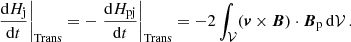 (16)
(16)
These volume terms have opposite signs: they correspond to terms of transfer of helicity between Hj and Hpj. Linan et al. (2018) have thus found that, unlike magnetic helicity, Hj and Hpj are not conserved quantities, and they have highlighted the existence of a gauge-invariant volume term that acts to convert Hj into Hpj and inversely.
In ideal MHD, the dissipation terms are strictly null. Even when non-ideal effects such as magnetic reconnection are present, the dissipation of magnetic helicity is thought to be very limited (Berger 1984; Pariat et al. 2015b). Similar to the simulation of Pariat et al. (2009), the simulations studied here are modelled with the ARMS solver without explicit resistivity but with an adaptive mesh refinement strategy, which increases the resolution at current sheets, where magnetic dissipation is the largest. Analysing the jet simulation of Pariat et al. (2009), Pariat et al. (2015b) demonstrated that the dissipation of relative magnetic helicity, HV was extremely limited (below 2%), even when intense magnetic reconnections or reconfiguration of the system was ongoing. Following Linan et al. (2018), we verified that the dissipation of Hj and Hpj was also very limited in the presently studied simulations. In such cases, the evolution equations of Hj and Hpj can thus be limited to:
 (17)
(17)
 (18)
(18)
Following Linan et al. (2018 cf. Sect. 3.4), we assessed the validity of the assumption of near ideality. We measured the difference between the time derivative of Hj and Hpj with the direct estimation of dHj/dt and dHpj/dt in both simulations. We found that the relative error was at most 7%, which remains very small. This is in the range of what was obtained in Linan et al. (2018) for the different MHD simulations analysed. The main differences occur during the period of strong evolution of dHj/dt and dHpj/dt, and thus the difference likely results mainly from the relatively low cadence of the data, which does not permit us to optimally evaluate the time derivative of Hj and Hpj. Overall we are confident that the dissipation of helicities remains negligible in comparison to the other terms.
3.5. Methods to estimate energies and helicities
In order to compute the different helicities and energies at each time in the simulation, we followed the procedure of Valori et al. (2012, 2013), and Linan et al. (2018). We focused our analysis on data cubes of B and v extracted from the adaptive mesh grid of each simulation. The data cubes were extracted on a regular grid in a sub-volume with x ∈ [0, 10.8] and y and z ∈ ±5.8. In both simulations the grid within this volume had a fixed minimum of four levels of refinement (see Fig. 3 in Wyper et al. 2018). The regular grid for the data cubes was coincident with this uniform local grid. In the jet-producing case, this led to a slight coarsening of the grid in places where the grid adaptively refined to one level higher. As they were integral quantities, and as shown in (Pariat et al. 2015b), this had a negligible effect on the helicities.
The time sequence of data cubes of the magnetic field B permitted us to compute all the magnetic energies and magnetic helicities of Eqs. (5) and (9). First, the scalar potential ϕ was obtained from a numerical solution of the Laplace equation (cf. Eq. (2)). The solenoidal potential field Bp and the solenoidal non-potential field Bj were derived following Valori et al. (2013 see Sects. 3.1 and 3.2). These fields permitted us to derive the different energies of Eq. (5) and in particular Etot, Efree, Epot, and Ediv (Eq. (6)).
In order to compute the helicities, the potential vectors A and Ap were then estimated using the DeVore-Coulomb gauge defined in Pariat et al. (2015b), based on Eq. (14) of Valori et al. (2012). Given that the system was a solar-like active region, with more intense magnetic field at the bottom boundary, following previous practice, the 1D integration involved was started from the top of the domain in order to minimise errors (cf. discussions in Pariat et al. 2015b, 2017). The gauge used to compute the potential vectors was fully fixed. From the derived potential vectors, we obtained the helicities, HV, Hj, and Hpj from Eqs. (9) and (11). As a sanity check, we also performed the computation in a different gauge (see e.g. Pariat et al. 2017, for other gauge choices). Given the low solenoidality of the magnetic field (low Ediv, cf. Sect. 3.1), we found no noticeable difference between the computation performed in the different gauges.
The computation of the time variations of Hj and Hpj could be then done independently from the estimations of the volume helicities (Linan et al. 2018, 2020). In addition to the knowledge of the magnetic fields (B, Bp and Bj) and from the estimation of their vector potential (A, Ap and Aj), the estimation of the terms of Eqs. (17), (18) required the knowledge of the data cubes of the plasma-velocity field v, which was extracted from the simulation similarly to B. This allowed us to determine, dHj/dt|Own, dHpj/dt|Own, dHpj/dt|Trans, dHj/dt|Trans, and their sum dHj/dt and dHpj/dt.
All these quantities were computed in both simulations, at each time step. This permitted us to finely analyse the dynamics of the magnetic energies and of the helicities in the jet-producing simulation, and compare it with the non-eruptive one.
4. Dynamics of magnetic energies and helicities in the simulations
In this section, we describe the evolution, in both the non-eruptive and the jet-producing simulation, of the different magnetic energies and helicities, as determined by the methods described in Sect. 3.5. The focus being on the pre-eruptive phase, the description of the energies and helicity evolution during the jet (for the jet-producing simulation) will only be reviewed briefly, without going into details.
4.1. Evolution of magnetic energies
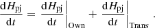
The evolution of the total magnetic energy, Etot, of the potential energy, Epot, and of the free magnetic energy, Efree, is presented in the top panel of Fig. 4, and the values at a few selected times are given in Table 1. Because of their very low value, thanks to the excellent solenoidality of B (cf. Sect. 3.1), the solenoidal terms entering in the decomposition of Etot (cf. Eq. (5)) are not represented.
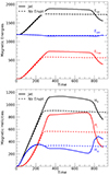 |
Fig. 4. Time evolution of the magnetic energies and helicities. Top panel: evolution of the total magnetic energy (Etot, black lines), potential magnetic energy (Epot, blue lines), and free magnetic energy (Efree, red lines) in the non-eruptive (dashed lines) and in the jet-producing (continuous lines) simulations. Bottom panel: evolution of the total relative magnetic helicity (HV, black lines), non-potential magnetic helicity (Hj, red lines), and volume-threading magnetic helicity (Hpj, blue lines), in the non-eruptive (dashed lines) and in the jet-producing (continuous lines) simulations. |
Values of magnetic energies and helicities, and some of their ratios at different instants of the simulations.
By design the field is initially potential, and one has Etot(t = 0)=Epot(t = 0) and Efree(t = 0)=0. Thanks to the bottom-boundary driving motions, free magnetic energy is injected in the system. During the common driving phase, Efree monotonically (and almost linearly) increases in both simulations. Meanwhile, Epot very slightly decreases, with (Epot(t = 300)−Epot(t = 0))/Epot(t = 0)∼0.02. By design of the driving pattern in the simulations, the vertical component of B is kept fixed. One could believe that Epot would remain constant. However, the forcing enhances the transverse field in the close-field domain. Because of the increase in the magnetic pressure, the closed-field domain bulges, slightly pushing the open field. The distribution of the normal component to the side boundaries of the system are thus slightly changing, inducing the observed small evolution of Epot. This variation is, however, very small compared to the injection of Efree, and Etot therefore steadily increases during the driving phase.
At t = 300, at the end of the forcing for the non-eruptive simulation, Efree represents 34% of Etot (cf. Table 1). At the same instant, Efree/Etot ∼ 37% for the jet-producing simulation. This value is slightly larger for the jet-producing case because the driving motion has been ramped down earlier for the non-eruptive run.
During the post-driving phase of the non-eruptive simulation, Epot remains basically constant (within 0.3%). The non-potential energy Efree very slightly decreases (see top panel of Fig. 4). The relative decrease by the end of the non-eruptive simulation is of the order of 3–4%. This decrease is likely due the low-intensity reconnection and the mild reconfiguration taking place in the system during that phase. Accordingly, Etot also decreases but this only corresponds to about 1% of relative variation. As can be noted in Table 1, the ratio of the free energy to the total energy remains constant during this post-driving phase for the non-eruptive simulation.
The jet-producing simulation is driven until t = 350, and thus benefits from a larger energy input. The peak value of Efree is about 26% higher for the jet-producing simulation than for the non-eruptive simulation. At t = 360 just after the end of the forcing, the ratio of the free energy normalised by the total energy has reached 0.39, which is about 15% higher than the maximum ratio of the non-eruptive simulation.
As with the non-eruptive simulation, the reconnection and the reconfiguration occurring during the post-driving phase induces a decrease in Efree and Etot (while Epot stays almost constant). However, since the reconnection dynamics has a stronger intensity in the jet-producing simulation, the decrease is more marked in absolute value: Etot and Efree decreases by about 30 energy units between t = 360 and t = 740. However, since the jet-producing simulation had a larger free energy content, in relative value, Efree and Etot respectively decrease by 4% and 1.6%. This relative variation is thus very similar to the energy change observed during the post-driving phase of the non-eruptive simulation. In terms of energy, the reconfiguration in the post-driving phase relatively impacts the system in a similar way.
Finally, after t ≃ 750, the onset of the jet is characterised by a sudden decrease in Efree, as magnetic energy is dissipated and partly converted to kinetic energy. Epot displays only weak variations, due to the small change in the magnetic flux distribution on the side and top boundaries.
4.2. Evolution of magnetic helicities
The evolution of the total magnetic helicity, HV, of the non-potential helicity Hj and of volume-threading helicity, Hpj is presented in the bottom panel of Fig. 4. Their values at a few selected times are given in Table 1. The initial configuration being potential, the system is void of helicity and the three helicities are null at t = 0. During the common driving phase, with shear and twist being injected, the total helicity monotonically increases. Unlike for magnetic energy, for which the increase was directly due to the injection of free magnetic energy, Efree, the helicity injection presents three phases. First, between t = 0 and t = 75, HV grows mainly due to the increase in Hpj, while Hj very mildly increases. Then, between t = 75 and t = 150, Hj starts to increase and HV grows thanks to the increase in both Hj and Hpj. The growth of Hpj, however, becomes weaker and weaker, eventually reaching a maximum around t ∼ 200 and and then even starts to decrease. Hence, between t = 150 and t = 300, the increase in HV is primarily due to Hj. It is worth noticing that the same dynamics of helicities were noted for the jet simulation analysed in Linan et al.(2018 see Fig. 3): HV grew first thanks to Hpj, which eventually later decreased, while Hj became the dominant contributor to HV. The analysis of the helicity fluxes, detailed in Sect. 4.3, allows to better understand this evolution.
For the non-eruptive simulation, during the post-driving phase, the dynamics of the helicities is in agreement with the evolution of the energies. All three helicities very weakly decrease: between t ∼ 350 and t ∼ 900, HV, Hj, and Hpj display a relative variation lower than 3%. This decrease is in line with the variation in Efree (and Etot) observed in the same period, and likely due to the weak-intensity reconnections occurring then.
On the contrary, the helicities in the jet-producing simulation present sensible variations that were not observed with the energies during the post-driving phase. Even though the bottom-boundary forcing has been halted, one observes a further decrease in Hpj and an increase in Hj. Between t = 360 and t = 700, Hj has a relative increase of 4%. This increase, while not as strong as during the driving phase, is relatively constant and is strikingly in opposition to the observed decrease in Efree during the same period. The dynamics of HV is, however, mostly dominated by the decrease in Hpj during this phase. While Hpj is roughly constant between t = 360 and t = 460, one observes a strong constant decrease between t = 460 and t = 740: Hpj presents a relative variation of 27%. HV thus similarly decreases. This evolution is present while no external forcing is applied to the system. The origin of this evolution is likely related to the important magnetic reconfiguration observed within the magnetic system of the jet-producing simulation. During this phase, the jet-producing simulation witnesses both a more intense and a longer current sheet at the null point, with more reconnection allowing strapping closed field lines to open, and simultaneously a more intense current sheet beneath the flux rope, inducing both a strengthening in the flux of the flux rope and its rise. In the present numerical experiment, helicities, as global scalar quantities cannot discriminate which dynamics (if not both) are responsible for the decrease in Hpj. In any case, the magnetic helicities thus appear to be much more sensitive to the magnetic reconfiguration observed in the system than the magnetic energies. Hpj presents a dynamic that is even more strongly marked as the system gets closer to the jet generation phase.
After t = 740, the helicities dynamics in the jet-producing simulation is evidently marked by the eruptive process. Similar to Efree, Hj decreases strongly. Meanwhile Hpj first markedly increases and then decreases. HV is dominated by the strong decrease in Hj and also diminishes.
Overall, while the driving phase shows similarities between the energies and helicities dynamics, the post-driving phase displays very distinct behaviours. While energies do not display significant evolution, both for the eruptive and the non-eruptive simulations, the helicities clearly discriminate the two numerical experiments. While the non-eruptive simulation does not display significant changes during the post-driving phase, the jet-producing simulation is marked by variations in the helicities. Hence, unlike the energies, the helicities are able to capture the reconfiguration of the system that occurs in the post-driving phase of the jet-producing simulation. The helicities are thus able to uniquely capture key dynamics of the magnetic system to which the energies are blind.
4.3. Hpj and Hj conversion
The analyses of the time variations of Hj and Hpj allow us to better understand the dynamics of helicity in the simulations. Fig. 5 presents the different terms of Eqs. (17), (18) for each simulation.
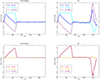 |
Fig. 5. Evolution of the terms of the time variation equation of Hpj (Eq. (18), top panels) and Hj (Eq. (17), bottom panels) for the non-eruptive (left column) and the jet-producing (right column) simulations: dHpj/dt (blue line), dHpj/dt|Own (cyan line), dHj/dt (red line), dHj/dt|Own (orange line), and dHpj/dt|Trans = −dHpj/dt|Trans (dashed purple lines). |
4.3.1. Driving phase
Starting with the evolution of dHj/dt during the driving phase of the non-eruptive simulation (upper left panel of Fig. 5), one sees that the initial increase in Hpj results first from dHpj/dt|Own, that is to say, from the injection of Hpj thanks to the boundary forcing motions. The curve of dHpj/dt|Own follows the boundary driver, first with an increase between t = 0 and t = 50 as the boundary motions are ramped up, then a constant intensity before being ramped down between t = 250 and t = 300. While dHj/dt|Trans is initially null until t ∼ 50, it then presents increasing negative values until t = 250. This means that Hpj is being converted into Hj. As a consequence, one observes in Fig. 4 (lower panel) that Hpj first increases (dashed blue line). While the injection of Hpj is initially dominant, as dHj/dt|Trans becomes more and more intense, dHpj/dt becomes weaker and weaker. The increase in Hpj is thus being reduced, as is noted in the lower panel of Fig. 4 (dashed blue line), reaching a maximum near t ∼ 200. For a short period, around t ∼ 250, dHj/dt|Trans even becomes dominant over dHpj/dt|Own (cf. Fig. 5) : Hpj is transferred faster into Hj than its injection by the boundary motion: the curve of Hpj (cf. Fig. 4, lower panel) thus slightly decreases.
The time evolution of Hj during the driving phase of the non-eruptive simulation is very different from the one of Hpj (see lower left panel of Fig. 5). There is basically no injection of Hj thanks to the boundary driving motions: dHj/dt|Own is constantly null. The variations of dHj/dt are exclusively due to dHj/dt|Trans, meaning that Hj is uniquely formed thanks to the conversion from Hpj. Since dHj/dt|Trans is regularly increasing (having the opposite sign of dHpj/dt|Trans), Hj rapidly increases, as observed in the lower panel of Fig. 4 (dashed red line), although the rise of Hj is delayed compared to Hpj. As the boundary driving motions are ramped down, the conversion of Hpj stops and the increase in Hj is drastically reduced.
For the non-eruptive simulations, for t > 300, during the post-driving phase, all helicity variation terms are very small in comparison to the driving phase (left panels of Fig. 5). They are close to zero, although not completely null, as will be discussed later. From then on, Hj and Hpj remain almost constant after t = 300 for this non-eruptive case.
The helicity dynamics for the jet-producing simulation is completely equivalent to the non-eruptive one during the driving phase (cf. right panels of Fig. 5). The curves of dHpj/dt, dHj/dt, and their decomposition present the same overall shape and intensity. The main difference between the two simulations during this driving phase is the longer driving time. The primary source of helicity comes from dHpj/dt|Own, which generates an increase in Hpj (initial positive values of dHpj/dt). However, Hpj is converted into Hj and this conversion process eventually dominates dHpj/dt, which becomes negative. Hpj thus decreases. Because of the longer driving, the decrease inHpj is more marked in the jet-producing simulation compared to the non-eruptive one (see lower panel of Fig. 4, continuous blue line). The non-potential helicity Hj also does not present proper injection (dHj/dt|Own is almost null) and Hj is exclusively formed by conversion from Hpj. Thanks to the longer driving time in the jet-producing simulation, Hj benefits from a longer time for conversion from Hpj, and can thus reach larger values than in the non-eruptive case (Fig. 4, lower panel, continuous red line). This dynamics is fully consistent with the results of the analysis of the helicity dynamics of a jet simulation by Linan et al. (2018, cf. Fig. 11).
4.3.2. Post-driving phase
While the dynamics of Hj and Hpj are very similar for both simulations during the driving phase, strong differences appear between the two cases during the post-driving phase, between t = 350 and t = 700. In order to better see the time variations of Hj and Hpj, Fig. 6 presents a zoomed-in view of the evolution of dHpj/dt and dHj/dt during the post-driving phase for each simulation. Three main differences can be noted between the jet-producing case and the non-eruptive simulation: dHj/dt|Trans (and dHpj/dt|Trans) has an opposite sign in the two simulations, its intensity is about twice larger for the jet-producing simulation, and dHpj/dt is also significantly higher in the jet-producing case.
For the non-eruptive simulation, during the post-driving phase, dHpj/dt|Trans is constantly positive with an intensity lower than 0.1 (cf. upper left panel of Fig. 6). This implies a small conversion of Hj into Hpj. Meanwhile dHpj/dt|Own oscillates and is, on average, slightly negative. This corresponds to a small ejection of Hpj through the side boundaries while the magnetic system is slowly reconfiguring. As a result, dHpj/dt oscillates around zero, and hence Hpj is constant. Since dHj/dt|Own is almost null (Fig. 6, lower left panel), similarly to the driving phase, dHj/dt is equal to dHj/dt|Trans (i.e. −dHpj/dt|Trans), meaning a slow transfer of Hj into Hpj. This conversion is sufficiently small as to be barely discernible in the curve of Hj during the post-driving phase of the non-eruptive simulation (Fig. 4, lower panel, dashed red line).
The time variations of Hj and Hpj are very different for the jet-producing simulation. Instead of being positive, dHpj/dt|Trans is negative during the post-driving phase of the jet-producing simulation (cf. upper right panel of Fig. 6). Respectively, instead of being negative in the non-eruptive case, dHj/dt|Trans is here positive (Fig. 6, lower right panel). Similarly to the non-eruptive simulation, dHj/dt|Own is almost null and dHpj/dt|Own is overall negative. As in the non-eruptive simulation, there is no proper injection of Hj and Hpj is ejected from the system though the side boundaries. However, the intensity of dHpj/dt|Own is about twice larger in the jet-producing case compared to the non-eruptive case (Fig. 6, top panels). Contrary to the non-eruptive case, since dHpj/dt|Own and dHpj/dt|Trans have the same negative sign for the jet-producing case, dHpj/dt is markedly negative, which corresponds to a sensible decrease in Hpj during this post-driving phase (cf. continuous blue line in the lower panel of Fig. 4).
The intensity of dHj/dt|Trans is about 0.2 for the jet-producing simulation, which is about twice the intensity in the non-eruptive case (Fig. 6, bottom panels). Rather than a conversion of Hj into Hpj, the post-driving phase is marked by a further conversion of Hpj into Hj. The conversion that was already ongoing during the driving phase continues, although at a slower rate. In the post-driving phase of the jet-producing simulation, Hj is thus further rising (cf. Fig. 4, lower panel, continuous red line).
The reconfiguration of the magnetic system that is observed during the post-driving phase of the jet-producing simulation (cf. Sect. 2.4) is thus fundamentally different from the one happening in the non-eruptive simulation. While in the non-eruptive case, the reconfiguration induces a minor decrease in Hj, which is transformed into Hpj, which is in turn ejected out of the domain, in the eruptive simulation, Hpj is partly ejected and partly transformed into Hj. The evolution induced simultaneously by the intense null-point reconnection, the reconnection beneath the flux rope, and the rise of the flux rope, impact the helicity distribution of the jet-producing simulation, without it being possible to causally link each system dynamics to a specific helicity evolution. The non-potential helicity Hj thus rises while Hpj decreases: this naturaly leads to an evolution of the helicity eruptivity index ηH, as is discussed in Sect. 4.4.
Finally, during the jet-generation phase of the jet-producing simulation (i.e. for t > 750), Hpj and Hj present strong variations (cf. right panels of Fig. 5). The evolution during that phase is completely similar to the jet simulation of Pariat et al. (2009) that has been analysed in Linan et al. (2018 cf. Fig. 11). Hj first and mainly decreases because it is converted into Hpj: dHj/dt|Trans presents a strong negative peak. Hj thus increases (positive dHpj/dt) thanks to a positive dHpj/dt|Trans. However, the increase in Hpj is quickly altered as a strong ejection of Hpj (negative dHpj/dt|Own) develops. After t ∼ 840, dHpj/dt|Own overcomes dHj/dt|Trans and dHpj/dt becomes negative: both Hj and Hpj decrease. As noted in Linan et al. (2018), Hj is not directly ejected but is first converted in Hpj and the later is ejected out of the simulation domain. This is the inverse process of what occurred during the driving phase, although occurring faster and more impulsively.
4.4. Helicity eruptivity index
The evolution of the helicity eruptivity index, ηH = Hj/HV (Eq. (12)), is displayed in the middle panel of Fig. 7. Its values at a few selected times are given in Table 1.
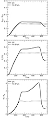 |
Fig. 7. Time evolution of non-dimensional quantities in the non-eruptive (dashed lines) and jet-producing (continuous lines) simulations: Efree/Etot (top panel), helicity eruptivity index ηH = Hj/HV (middle panel), and Hj/Hpj (bottom panel). |
For the non-eruptive simulation, ηH steadily increases during the driving phase until reaching 0.63 at t = 300 and then it stays constant. For the jet-producing simulation, ηH reaches 0.74 at the end of its driving phase, at t = 360. At the end of the driving phase, ηH thus first presents a larger value (by 17%) for the jet-producing simulation compared to the non-eruptive one. This is to be compared with the free energy ratio, Efree/Etot (see top panel of Fig. 7 and Table 1), whose maximum is also about 17% higher for the jet-producing simulation, relatively to the non-eruptive simulation.
In the post-driving phase, while for the non-eruptive simulation both ηH and Efree/Etot remain constant, the evolution of the helicity eruptivity index significantly differs from the free energy ratio for the jet-producing simulation. Once the driving has stopped, Efree/Etot very slowly decreases. There is no significant evolution between the end of the forcing at t = 350 and the generation of the jet after t ∼ 750. On the contrary, ηH further increases. Following the sensitive increase in Hj and the decrease in Hpj (cf. Sect. 4.2), ηH goes from 0.74 at t = 360 to 0.8 at t = 740, before the generation of the jet. Said differently, at the onset of the jet, Hj represents 80% of the helicity content of the system. The helicity eruptivity index is at its peak value just before the onset of the eruptive behaviour. During the generation of the jet, ηH decreases and its value falls even below the value of the non-eruptive simulation.
The increase in the helicity eruptivity index reveals the increasingly dominating role that Hj has in HV. Another way to see this is to follow the ratio Hj/Hpj, as presented in Fig. 7. We note that for the non-eruptive case, at the end of the driving phase, Hj is about 1.7 times larger than Hpj. In the case of the jet-producing simulation, Hj is about three times larger (2.88 at t = 360) than Hpj at the end of the driving phase. This fraction further increases by 41% during the post driving phase to reach Hj/Hpj = 4.07 at t = 740. The Hj/Hpj ratio presents a relative difference that is almost as important between the end of the driving phase and the onset of the jet as the relative difference between the non-eruptive case and the jet-producing case at the end of their respective driving phase. Again, the careful analysis of the helicity content clearly reveals the important reconfiguration dynamics occurring in the system, which the magnetic energy is not able to capture.
It is interesting to see the role of Hj in conjunction with the eruptive behaviour. Figure 7 shows that at the onset of the generation of the jet, the relative helicity of the system is dominated by the non-potential helicity Hj. This behaviour is also observed in other numerical models. For example, the jet-producing simulation of Pariat et al. (2009) analysed in Linan et al. (2018) presented a similar decrease in Hpj as the system got closer to the instability. Actually, in that simulation, Hpj even changed sign and had a chirality opposite to Hj and HV (cf. Fig. 3 of Linan et al. 2018). The helicity eruptivity index was thus larger than 1 at the onset of the jet. In the flux emergence simulations of Leake et al. (2013, 2014) studied in Pariat et al. (2017), eruptions were generated for the systems that had the lower amount of Hpj. The eruptions were triggered the earliest in the systems which that contained an amount of Hpj of opposite sign to Hj. It is therefore puzzling to see in the present study that not only was ηH higher after the point of no return, that is to say, higher at the end of the driving phase of the jet-producing case (versus the non-eruptive case), but that during the post-driving phase, ηH was further increasing, meaning that Hj was further dominating Hpj as the system was approaching the actual eruption and the generation of the jet. This highlights again the fact that helicities, Hj, Hpj, and ηH, seem to be tightly linked with the eruptive dynamics of solar-like active magnetic systems.
5. Conclusions and discussion
5.1. Summary
The present study is focussed on understanding the possible link between magnetic helicity and the eruptivity of solar-like magnetic systems. Here, we have analysed the magnetic energy and helicity dynamics in two parametric 3D MHD numerical simulations that can induce solar coronal jets (cf. Sect. 2). In both simulations, the initial magnetic system is composed of a single 3D null-point topology, dividing the domain into a closed-field region (below the fan dome of the null point) and an open-field region. In both cases, the system is driven by line-tied boundary motions inside the closed domain, in order to form a flux rope initially contained within the closed domain (cf. Sect. 2.2).
In one simulation (cf. Sect. 2.4), presented and analysed in Wyper et al. (2018), the system is driven sufficiently that a point of no return is reached for the stability of the system : a jet is eventually generated following previous simulation results (Pariat et al. 2009, 2015a, 2016; Wyper et al. 2017). Interestingly, the onset of the jet does not occur during or immediately after the driving phase in this simulation. The onset phase of the jet is significantly delayed after the end of the driving phase. During this post-driving phase, (labelled ‘breakout phase’ in Wyper et al. 2018), the flux rope presents a steady evolution involving reconnection, which while sustained is not eruptive or exponentially growing. During this phase, a reconfiguration of the magnetic field takes place: a fraction of the closed-field magnetic flux becomes part of the flux rope, increasing its flux, while simultaneously the strapping field linking with it is removed. In a new simulation (cf. Sect. 2.3), the system is driven during a shorter time compared to the previously analysed one. During this shorter driving period, the point of no return for the generation of the jet is not reached. The post-driving phase continues and is not followed by the onset of a jet. While some reconnection is present during the post driving phase, the flux rope created during the driving phase remains stable.
Because of their distinct behaviour, it is particularly interesting to analyse the properties of the different magnetic energies and helicities (cf. Sect. 3). We looked more specifically at the dynamics of the non-potential magnetic helicity, Hj (Eq. (11)), of the volume-threading magnetic helicity, Hpj (Eq. (11)), and of the helicity eruptivity index, ηH (Eq. (12)). The latter has been found in a few recent numerical models, as well as in observations of solar active regions to mark the eruptivity of the system Pariat et al. (2017), Zuccarello et al. (2018), Linan et al. (2018), Moraitis et al. (2019b), Thalmann et al. (2021), Gupta et al. (2021), and Green et al. (2022).
The main results of our analysis are (cf. Sect. 4):
-
The driving motions during the driving phase induces the injection of free magnetic energy, Hj and Hpj, and hence the increase in both total magnetic energy and helicity. Since the driving phase lasts longer, more free energy, Hj, total magnetic energy, and helicity are injected in the jet-producing simulation. The jet-producing simulation is thus associated with a larger amount of Etot, Efree, Hj, and Hpj compared to the non-eruptive one, as expected from classical solar eruption theory.
-
However, the volume-threading helicity, Hpj, is smaller at the end of the driving phase of the jet-producing case compared to the end of the driving phase of the non-eruptive case. The additional forcing, during which the point of no return is crossed, is coincident with this decrease in Hpj.
-
During the post-driving phases, Efree and Etot very slightly decrease in both simulations. Unlike magnetic energies, magnetic helicities are sensitive to the reconfiguration occurring in the post-driving phase of the jet-producing simulation. The fluxes of Hj and Hpj present completely distinct behaviours in each simulation during the post-driving phase (cf. Sect. 4.3). The helicities are thus able to uniquely capture key dynamics of the magnetic system to which the magnetic energies are blind.
-
During the post driving phases of the jet-producing simulation, Hj and ηH further increase. The onset of the jet is thus associated with peak values of Hj, ηH, and Hj/Hpj (cf. Sect. 4.4). These quantities are sensitively higher at the dawn of the onset of the jet compared to the end of the driving phase.
5.2. Discussion
The first main outcome of this study relates to the comparative properties of magnetic helicity versus magnetic energy. As was already discussed in Linan et al. (2020), magnetic helicities appear to be significantly more sensitive quantities to the pre-eruptive properties of the magnetic system than magnetic energies. It is remarkable that magnetic energies are completely blind to the restructuring during the post-driving phase of the jet-producing simulation, while magnetic helicities do capture this evolution. It will also be worth investigating in a future study how the different restructuring dynamics (e.g. reconnection at the null point, reconnection below the flux rope, and the rise of the flux rope) relate to the different observed changes in helicities.
Another feature worth mentioning, which likely requires further studies, is the fact that magnetic helicities seem to change earlier that magnetic energies before the onset of the eruptive dynamics. Indeed, one observes that Hj (resp. Hpj) presents a maximum (resp. local minimum) at t = 740 (see Fig. 4). The decrease in the total and free magnetic energy related to the eruptive behaviour only becomes observable after t > 760. More strikingly, when looking at the fluxes (see Fig. 6) of Hj and Hpj, one observes that the transfer of helicity between Hj and Hpj reverts as early as t = 700. This obvious change in the helicity dynamics is likely related to the onset of the generation of the jet. Helicities and their fluxes may thus constitute a warning for the imminent onset of eruptive events.
The second major outcome of the present analysis relates to the potential use of the helicity eruptivity index, ηH, in eruption prediction. The numerical experiments of Zuccarello et al. (2018) clearly showed that the onset of the eruptive behaviour was associated with a threshold in ηH. Unlike in Zuccarello et al. (2018), where the point of no return was precisely determined, the present parametric simulations do not permit us to completely link the moment in which the system becomes unstable with the helicities. Although the behaviour during the post-driving phase heavily involves breakout reconnection above the flux rope structure (Wyper et al. 2017, 2018), the present simulations do not enable the precise determination of which instability triggers this eruptive behaviour, namely whether it is a resistive instability, as argued by the ‘breakout’ scenario (Antiochos et al. 1999), or an ideal MHD instability, such as the Torus instability (Kliem & Török 2006; Aulanier et al. 2010), which acts to kick off or to later supplement the eruptive evolution. Precisely determining this would require further parametric MHD simulations, perhaps alongside the use of an ideal code (e.g. Rachmeler et al. 2010), which is beyond the scope of this investigation. What can be strictly said is that a point of no return is crossed during the extra driving time of the jet-producing simulation, between t = 300 and t = 350, which eventually leads to the eruptive behaviour.
The observed delay between the point of no return and the actual onset of the jet is, however, of high interest. Two scenarios can be hypothesised, which present numerical experiments cannot discriminate. In the first scenario, the trigger of the eruptive behaviour occurs during the supplementary driving time of the jet-producing simulation. The post-driving phase can thus be viewed as a ‘linear’ phase of the loss of equilibrium that inevitably leads to the eruptive generation of the jet. The jet onset after t ∼ 740 is then simply the exponential phase of the development of the instability initiated between t = 300 and t = 350. In the present simulation, the linear phase is particularly long, enabling its analysis in detail. Since ηH is higher for the jet-producing case than the non-eruptive case in this time period, this scenario does not contradict that ηH is related to the instability trigger.
In a second alternative scenario, the point of no return is not directly associated with the trigger of the instability at the origin of the eruptive behaviour. The point of no return may here be associated with a first instability that induces the reconfiguration of the magnetic closed system with the further build-up of a flux rope. Doing so, helicity is further converted from Hpj to Hj in the jet-producing case, in opposition to the non-eruptive case. As the magnetic system reconfigures itself, and ηH further rises, the system may be driving towards a second instability (ideal or not), this one directly associated with the onset of the eruption or jet. If ηH is indeed associated with such eruptive instability, this would explain why the system erupts only after t > 740 and not directly at the end of the driving phase. The critical ηH threshold may not yet have been reached at t = 350 and it is only thanks to the reconfiguration in the post-driving phase that ηH reaches the instability threshold level.
Whichever scenario is correct, this study further confirms the results of Pariat et al. (2017), Zuccarello et al. (2018), and Linan et al. (2018, 2020), pointing towards a tight link between the eruptivity of magnetic configurations and magnetic helicities, and in particular the helicity eruptivity index ηH. Similar to the previously analysed simulations, we find in the present simulation that ηH is higher for the jet-producing simulation compared to the non-eruptive case, that ηH presents a peak just before the onset of the eruptive jet, and that the value of ηH decreases once the eruption or jet occurs.
However, the nature of the causal link between ηH and the trigger of the eruptions still needs to be determined. Pariat et al. (2017) and Zuccarello et al. (2018) suggested that ηH is related to the torus instability. Recently Kliem & Seehafer (2022) showed that kink and torus unstable systems were very efficient at shedding magnetic helicity, and in particular Hj, while Hpj was only partly extracted. They found that the systems were stable when ηH lied below a certain threshold. This study highlights the possible link between ηH and the torus instability.
The search for the causal link between the properties of the pre-eruptive magnetic field and the trigger of active solar events is an extremely dynamic topic in solar physics (e.g. Leka et al. 2019a,b; Park et al. 2020; Georgoulis et al. 2021). Innovative quantities permitting a prediction for eruptive events are being looked for. Magnetic twist, winding, and helicity, which all relate to the level of entanglement and complexity of the magnetic field, seem to constitute a promising approach. In addition to the helicity eruptivity index that this study focusses on, other helicity-related quantities have very recently been proposed. Historically, multiple studies have focussed on the total helicity content (e.g. Nindos & Andrews 2004; LaBonte et al. 2007; Park et al. 2010; Tziotziou et al. 2012; Vemareddy 2019; Liokati et al. 2022). Recently, in a 2D parametric numerical study, Rice & Yeates (2022) found that major eruptions were best predicted by thresholds in the ratios of rope current to magnetic energy of helicity. They noted that the helicity eruptivity index was negatively correlated with eruptions. Li et al. (2022) have proposed using the ratio of a twist parameter to the total unsigned flux to distinguish large eruptive and confined flares. Building on the theoretical studies of Prior & MacTaggart (2020) and MacTaggart & Prior (2021), Raphaldini et al. (2022) have shown that magnetic winding could successfully indicate the flaring and eruptive activity in some active regions. All these results point to the importance of twist and helicity in the physics of solar eruption. Because of the inherent difficulties in measuring these quantities, and the tricky properties of some (e.g. the non-simple additivity of relative magnetic helicity Valori et al. 2020), large efforts must still be made to identify truly meaningful quantities for flare and eruption prediction.
Acknowledgments
We thank the anonymous referee for her/his thorough review of the manuscript. This project is a direct outcome of the visit of EP and TP at Durham University supported by the Alliance Hubert Curien Program funded by the french Ministère de l’Europe et des Affaires Etrangères and the Ministère de l’Enseignement Supérieur et de la Recherche, and managed by Campus France. This work was supported by the French Programme National PNST of CNRS/INSU co-funded by CNES and CEA. EP also acknowledges financial support from the French national space agency (CNES) through the APR program. LL acknowledges support from the European Union’s Horizon 2020 research and innovation programme under grant agreement NO 870405. The numerical simulations were sponsored by allocations on Discover at NASA’s Center for Climate Simulation and on the DiRAC Data Analytic system at the University of Cambridge, operated by the University of Cambridge High Performance Computing Service on behalf of the STFC DiRAC HPC Facility (www.dirac.ac.uk) and funded by BIS National E-infrastructure capital grant (ST/K001590/1), STFC capital grants ST/H008861/1 and ST/H00887X/1, and STFC DiRAC Operations grant ST/K00333X/1. DiRAC is part of the National E-Infrastructure.
References
- Aly, J.-J. 2018, Fluid Dyn. Res., 50, 011408 [Google Scholar]
- Antiochos, S. K., DeVore, C. R., & Klimchuk, J. A. 1999, ApJ, 510, 485 [Google Scholar]
- Aulanier, G., Pariat, E., & Démoulin, P. 2005, A&A, 444, 961 [NASA ADS] [CrossRef] [EDP Sciences] [Google Scholar]
- Aulanier, G., Pariat, E., Démoulin, P., & DeVore, C. R. 2006, Sol. Phys., 238, 347 [NASA ADS] [CrossRef] [Google Scholar]
- Aulanier, G., Török, T., Démoulin, P., & DeLuca, E. E. 2010, ApJ, 708, 314 [Google Scholar]
- Berger, M. A. 1984, Geophys. Astrophys. Fluid Dyn., 30, 79 [NASA ADS] [CrossRef] [Google Scholar]
- Berger, M. A. 2003, in Advances in Nonlinear Dynamics, eds. A. Ferriz-Mas, & M. Núñez, 345 [Google Scholar]
- Berger, M. A., & Field, G. B. 1984, J. Fluid Mech., 147, 133 [NASA ADS] [CrossRef] [Google Scholar]
- Chae, J. 2001, ApJ, 560, L95 [NASA ADS] [CrossRef] [Google Scholar]
- Chae, J. 2007, Adv. Space Res., 39, 1700 [NASA ADS] [CrossRef] [Google Scholar]
- Dalmasse, K., Pariat, E., Valori, G., Démoulin, P., & Green, L. M. 2013, A&A, 555, L6 [NASA ADS] [CrossRef] [EDP Sciences] [Google Scholar]
- Dalmasse, K., Pariat, E., Démoulin, P., & Aulanier, G. 2014, Sol. Phys., 289, 107 [NASA ADS] [CrossRef] [Google Scholar]
- Dalmasse, K., Pariat, E., Valori, G., Jing, J., & Démoulin, P. 2018, ApJ, 852, 141 [NASA ADS] [CrossRef] [Google Scholar]
- DeVore, C. R., & Antiochos, S. K. 2008, ApJ, 680, 740 [NASA ADS] [CrossRef] [Google Scholar]
- Démoulin, P. 2007, Adv. Space Res., 39, 1674 [CrossRef] [Google Scholar]
- Démoulin, P., & Pariat, E. 2009, Adv. Space Res., 43, 1013 [CrossRef] [Google Scholar]
- Démoulin, P., Priest, E. R., & Mandrini, C. H. 1996, A&A, 308, 643 [Google Scholar]
- Elsasser, W. M. 1956, Rev. Modern Phys., 28, 135 [NASA ADS] [CrossRef] [Google Scholar]
- Finn, J. H., & Antonsen, T. M. J. 1985, Comments Plasma Phys. Controlled Fusion, 9, 111 [Google Scholar]
- Georgoulis, M. K., Bloomfield, D. S., Piana, M., et al. 2021, J. Space Weather Space Clim., 11, 39 [CrossRef] [EDP Sciences] [Google Scholar]
- Green, L. M., Thalmann, J. K., Valori, G., et al. 2022, ApJ, 937, 59 [NASA ADS] [CrossRef] [Google Scholar]
- Guo, Y., Pariat, E., Valori, G., et al. 2017, ApJ, 840, 40 [NASA ADS] [CrossRef] [Google Scholar]
- Gupta, M., Thalmann, J. K., & Veronig, A. M. 2021, A&A, 653, A69 [NASA ADS] [CrossRef] [EDP Sciences] [Google Scholar]
- James, A. W., Valori, G., Green, L. M., et al. 2018, ApJ, 855, L16 [NASA ADS] [CrossRef] [Google Scholar]
- Kliem, B., & Seehafer, N. 2022, A&A, 659, A49 [NASA ADS] [CrossRef] [EDP Sciences] [Google Scholar]
- Kliem, B., & Török, T. 2006, Phys. Rev. Lett., 96, 255002 [Google Scholar]
- Knizhnik, K. J., Antiochos, S. K., & DeVore, C. R. 2015, ApJ, 809, 137 [NASA ADS] [CrossRef] [Google Scholar]
- Kumar, P., Karpen, J. T., Antiochos, S. K., et al. 2018, ApJ, 854, 155 [NASA ADS] [CrossRef] [Google Scholar]
- Kumar, P., Karpen, J. T., Antiochos, S. K., et al. 2019, ApJ, 873, 93 [NASA ADS] [CrossRef] [Google Scholar]
- LaBonte, B. J., Georgoulis, M. K., & Rust, D. M. 2007, ApJ, 671, 955 [CrossRef] [Google Scholar]
- Leake, J. E., Linton, M. G., & Antiochos, S. K. 2014, ApJ, 787, 46 [NASA ADS] [CrossRef] [Google Scholar]
- Leake, J. E., Linton, M. G., & Török, T. 2013, ApJ, 778, 99 [NASA ADS] [CrossRef] [Google Scholar]
- Leka, K. D., Park, S.-H., Kusano, K., et al. 2019a, ApJS, 243, 36 [NASA ADS] [CrossRef] [Google Scholar]
- Leka, K. D., Park, S.-H., Kusano, K., et al. 2019b, ApJ, 881, 101 [NASA ADS] [CrossRef] [Google Scholar]
- Li, T., Sun, X., Hou, Y., et al. 2022, ApJ, 926, L14 [NASA ADS] [CrossRef] [Google Scholar]
- Linan, L., Pariat, E., Aulanier, G., Moraitis, K., & Valori, G. 2020, A&A, 636, A41 [NASA ADS] [CrossRef] [EDP Sciences] [Google Scholar]
- Linan, L., Pariat, E., Moraitis, K., Valori, G., & Leake, J. 2018, ApJ, 865, 52 [NASA ADS] [CrossRef] [Google Scholar]
- Liokati, E., Nindos, A., & Liu, Y. 2022, A&A, 662, A6 [NASA ADS] [CrossRef] [EDP Sciences] [Google Scholar]
- Longcope, D. W. 2005, Liv. Rev. Sol. Phys., 2, 7 [Google Scholar]
- Low, B. C. 1996, Sol. Phys., 167, 217 [Google Scholar]
- Lumme, E., Pomoell, J., Price, D. J., et al. 2022, A&A, 658, A200 [NASA ADS] [CrossRef] [EDP Sciences] [Google Scholar]
- MacTaggart, D., & Prior, C. 2021, Geophys. Astrophys. Fluid Dyn., 115, 85 [NASA ADS] [CrossRef] [Google Scholar]
- Masson, S., Pariat, E., Aulanier, G., & Schrijver, C. J. 2009, ApJ, 700, 559 [Google Scholar]
- Masson, S., Pariat, E., Valori, G., et al. 2017, A&A, 604, A76 [NASA ADS] [CrossRef] [EDP Sciences] [Google Scholar]
- Moraitis, K., Tziotziou, K., Georgoulis, M. K., & Archontis, V. 2014, Sol. Phys., 122, 25 [Google Scholar]
- Moraitis, K., Pariat, E., Savcheva, A., & Valori, G. 2018, Sol. Phys., 293, 92 [NASA ADS] [CrossRef] [Google Scholar]
- Moraitis, K., Pariat, E., Valori, G., & Dalmasse, K. 2019a, A&A, 624, A51 [NASA ADS] [CrossRef] [EDP Sciences] [Google Scholar]
- Moraitis, K., Sun, X., Pariat, E., & Linan, L. 2019b, A&A, 628, A50 [NASA ADS] [CrossRef] [EDP Sciences] [Google Scholar]
- Nindos, A., & Andrews, M. D. 2004, ApJ, 616, L175 [NASA ADS] [CrossRef] [Google Scholar]
- Nindos, A., Zhang, J., & Zhang, H. 2003, ApJ, 594, 1033 [Google Scholar]
- Pariat, E., & Démoulin, P. 2012, A&A, 541, A78 [NASA ADS] [CrossRef] [EDP Sciences] [Google Scholar]
- Pariat, E., Démoulin, P., & Berger, M. A. 2005, A&A, 439, 1191 [NASA ADS] [CrossRef] [EDP Sciences] [Google Scholar]
- Pariat, E., Nindos, A., Démoulin, P., & Berger, M. A. 2006, A&A, 452, 623 [NASA ADS] [CrossRef] [EDP Sciences] [Google Scholar]
- Pariat, E., Antiochos, S. K., & DeVore, C. R. 2009, ApJ, 691, 61 [Google Scholar]
- Pariat, E., Dalmasse, K., DeVore, C. R., Antiochos, S. K., & Karpen, J. T. 2015a, A&A, 573, A130 [NASA ADS] [CrossRef] [EDP Sciences] [Google Scholar]
- Pariat, E., Valori, G., Démoulin, P., & Dalmasse, K. 2015b, A&A, 580, A128 [NASA ADS] [CrossRef] [EDP Sciences] [Google Scholar]
- Pariat, E., Dalmasse, K., DeVore, C. R., Antiochos, S. K., & Karpen, J. T. 2016, A&A, 596, A36 [NASA ADS] [CrossRef] [EDP Sciences] [Google Scholar]
- Pariat, E., Leake, J. E., Valori, G., et al. 2017, A&A, 601, A125 [CrossRef] [EDP Sciences] [Google Scholar]
- Park, S.-H., Chae, J., & Wang, H. 2010, ApJ, 718, 43 [NASA ADS] [CrossRef] [Google Scholar]
- Park, S.-H., Leka, K. D., Kusano, K., et al. 2020, ApJ, 890, 124 [NASA ADS] [CrossRef] [Google Scholar]
- Pevtsov, A. A., Berger, M. A., Nindos, A., Norton, A. A., & Driel-Gesztelyi, L. V. 2014, Space Sci. Rev., 186, 285 [NASA ADS] [CrossRef] [Google Scholar]
- Polito, V., Zanna, G. D., Valori, G., et al. 2017, A&A, 601, A39 [NASA ADS] [CrossRef] [EDP Sciences] [Google Scholar]
- Pontin, D., Galsgaard, K., & Démoulin, P. 2016, Sol. Phys., 291, 1739 [Google Scholar]
- Price, D. J., Pomoell, J., Lumme, E., & Kilpua, E. K. J. 2019, A&A, 628, A114 [NASA ADS] [CrossRef] [EDP Sciences] [Google Scholar]
- Priest, E. R., Longcope, D. W., & Janvier, M. 2016, Sol. Phys., 291, 1 [NASA ADS] [CrossRef] [Google Scholar]
- Prior, C., & MacTaggart, D. 2020, Proc. R. Soc. A, 476, 20200483 [NASA ADS] [CrossRef] [Google Scholar]
- Rachmeler, L. A., Pariat, E., DeForest, C. E., Antiochos, S., & Török, T. 2010, ApJ, 715, 1556 [NASA ADS] [CrossRef] [Google Scholar]
- Raouafi, N. E., Georgoulis, M. K., Rust, D. M., & Bernasconi, P. N. 2010, ApJ, 718, 981 [Google Scholar]
- Raphaldini, B., Prior, C. B., & MacTaggart, D. 2022, ApJ, 927, 156 [NASA ADS] [CrossRef] [Google Scholar]
- Rice, O. E. K., & Yeates, A. R. 2022, Front. Astron. Space Sci., 9, 849135 [NASA ADS] [CrossRef] [Google Scholar]
- Russell, A. J. B., Yeates, A. R., Hornig, G., & Wilmot-Smith, A. L. 2015, Phys. Plasmas, 22, 032106 [Google Scholar]
- Rust, D. M. 1994, Geophys. Res. Lett., 21, 241 [Google Scholar]
- Schuck, P. W., & Antiochos, S. K. 2019, ApJ, 882, 151 [Google Scholar]
- Shibata, K., & Uchida, Y. 1986, Sol. Phys., 103, 299 [NASA ADS] [CrossRef] [Google Scholar]
- Sterling, A. C., Moore, R., Falconer, D. A., & Adams, M. 2015, Nature, 523, 437 [Google Scholar]
- Taylor, J. B. 1974, Phys. Rev. Lett., 33, 1139 [Google Scholar]
- Temmer, M., Thalmann, J. K., Dissauer, K., et al. 2017, Sol. Phys., 292, 93 [NASA ADS] [CrossRef] [Google Scholar]
- Thalmann, J. K., Inhester, B., & Wiegelmann, T. 2011, Sol. Phys., 272, 243 [Google Scholar]
- Thalmann, J. K., Linan, L., Pariat, E., & Valori, G. 2019a, ApJ, 880, L6 [Google Scholar]
- Thalmann, J. K., Moraitis, K., Linan, L., et al. 2019b, ApJ, 887, 64 [Google Scholar]
- Thalmann, J. K., Sun, X., Moraitis, K., & Gupta, M. 2020, A&A, 643, A153 [EDP Sciences] [Google Scholar]
- Thalmann, J. K., Georgoulis, M. K., Liu, Y., et al. 2021, ApJ, 922, 41 [NASA ADS] [CrossRef] [Google Scholar]
- Thalmann, J. K., Gupta, M., & Veronig, A. M. 2022, A&A, 662, A3 [NASA ADS] [CrossRef] [EDP Sciences] [Google Scholar]
- Titov, V. S. 2007, ApJ, 660, 863 [Google Scholar]
- Titov, V. S., Hornig, G., & Démoulin, P. 2002, J. Geophys. Res. (Space Phys.), 107, 1164 [Google Scholar]
- Toriumi, S., & Park, S.-H. 2022, Ap&SS, submitted [arXiv: 2204.06010] [Google Scholar]
- Tziotziou, K., Georgoulis, M. K., & Raouafi, N.-E. 2012, ApJ, 759, L4 [NASA ADS] [CrossRef] [Google Scholar]
- Valori, G., Démoulin, P., & Pariat, E. 2012, Sol. Phys., 278, 347 [Google Scholar]
- Valori, G., Démoulin, P., Pariat, E., & Masson, S. 2013, A&A, 553, A38 [NASA ADS] [CrossRef] [EDP Sciences] [Google Scholar]
- Valori, G., Pariat, E., Anfinogentov, S., et al. 2016, Space Sci. Rev., 201, 147 [Google Scholar]
- Valori, G., Démoulin, P., Pariat, E., et al. 2020, A&A, 643, A26 [NASA ADS] [CrossRef] [EDP Sciences] [Google Scholar]
- Vemareddy, P. 2019, ApJ, 872, 182 [NASA ADS] [CrossRef] [Google Scholar]
- Wiegelmann, T., & Sakurai, T. 2012, Liv. Rev. Sol. Phys., 9, 5 [Google Scholar]
- Wiegelmann, T., Thalmann, J. K., & Solanki, S. K. 2014, A&ARv., 22, 78 [NASA ADS] [CrossRef] [Google Scholar]
- Woltjer, L. 1958, Proc. Nat. Acad. Sci., 44, 489 [Google Scholar]
- Wyper, P. F., Antiochos, S. K., & DeVore, C. R. 2017, Nature, 544, 452 [Google Scholar]
- Wyper, P. F., DeVore, C. R., & Antiochos, S. K. 2018, ApJ, 852, 98 [Google Scholar]
- Yang, K. E., Wheatland, M. S., & Gilchrist, S. A. 2020, ApJ, 894, 151 [NASA ADS] [CrossRef] [Google Scholar]
- Yeates, A. R., & Page, M. H. 2018, J. Plasma Phys., 84, 775840602 [Google Scholar]
- Zhao, J., Gilchrist, S. A., Aulanier, G., et al. 2016, ApJ, 823, 62 [Google Scholar]
- Zhao, L., DeVore, C. R., Antiochos, S. K., & Zurbuchen, T. H. 2015, ApJ, 805, 61 [NASA ADS] [CrossRef] [Google Scholar]
- Zuccarello, F. P., Aulanier, G., & Gilchrist, S. A. 2015, ApJ, 814, 126 [Google Scholar]
- Zuccarello, F. P., Pariat, E., Valori, G., & Linan, L. 2018, ApJ, 863, 41 [Google Scholar]
All Tables
Values of magnetic energies and helicities, and some of their ratios at different instants of the simulations.
All Figures
|
Fig. 1. Snapshots of the common initial phase (0 < t < 250) of both simulations. Left panels: electric current density distribution in a central 2D cut and magnetic field lines. Right: QSL distribution at t = 250. The dashed line shows the PIL. Top panels: non-eruptive case. Bottom panels: jet-producing case. Yellow shading indicates the open field. |
| In the text | |
|
Fig. 2. Snapshots at t = 350 and 800, for the non-eruptive simulation. Left panels: electric current density and field lines. Right panels: QSL distribution. Yellow shading indicates the open field. |
| In the text | |
|
Fig. 3. Snapshots at t = 350, 700, 760, and 850 for the jet-producing simulation. Left panels: electric current density and field lines. Right panels: QSL distribution. Yellow shading indicates the open field. |
| In the text | |
|
Fig. 4. Time evolution of the magnetic energies and helicities. Top panel: evolution of the total magnetic energy (Etot, black lines), potential magnetic energy (Epot, blue lines), and free magnetic energy (Efree, red lines) in the non-eruptive (dashed lines) and in the jet-producing (continuous lines) simulations. Bottom panel: evolution of the total relative magnetic helicity (HV, black lines), non-potential magnetic helicity (Hj, red lines), and volume-threading magnetic helicity (Hpj, blue lines), in the non-eruptive (dashed lines) and in the jet-producing (continuous lines) simulations. |
| In the text | |
|
Fig. 5. Evolution of the terms of the time variation equation of Hpj (Eq. (18), top panels) and Hj (Eq. (17), bottom panels) for the non-eruptive (left column) and the jet-producing (right column) simulations: dHpj/dt (blue line), dHpj/dt|Own (cyan line), dHj/dt (red line), dHj/dt|Own (orange line), and dHpj/dt|Trans = −dHpj/dt|Trans (dashed purple lines). |
| In the text | |
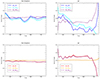 |
Fig. 6. Same as for Fig. 5, but focussed on the post-driving phase, between t = 350 and t = 750. |
| In the text | |
|
Fig. 7. Time evolution of non-dimensional quantities in the non-eruptive (dashed lines) and jet-producing (continuous lines) simulations: Efree/Etot (top panel), helicity eruptivity index ηH = Hj/HV (middle panel), and Hj/Hpj (bottom panel). |
| In the text | |
Current usage metrics show cumulative count of Article Views (full-text article views including HTML views, PDF and ePub downloads, according to the available data) and Abstracts Views on Vision4Press platform.
Data correspond to usage on the plateform after 2015. The current usage metrics is available 48-96 hours after online publication and is updated daily on week days.
Initial download of the metrics may take a while.