| Issue |
A&A
Volume 620, December 2018
|
|
|---|---|---|
| Article Number | A23 | |
| Number of page(s) | 10 | |
| Section | Stellar atmospheres | |
| DOI | https://doi.org/10.1051/0004-6361/201833745 | |
| Published online | 23 November 2018 | |
Spatially resolving the thermally inhomogeneous outer atmosphere of the red giant Arcturus in the 2.3 μm CO lines⋆
Instituto de Astronomía, Universidad Católica del Norte, Avenida Angamos 0610, Antofagasta, Chile
e-mail: This email address is being protected from spambots. You need JavaScript enabled to view it.
Received:
29
June
2018
Accepted:
30
August
2018
Abstract
Aim. The outer atmosphere of K giants shows thermally inhomogeneous structures consisting of the hot chromospheric gas and the cool molecular gas. We present spectro-interferometric observations of the multicomponent outer atmosphere of the well-studied K1.5 giant Arcturus (α Boo) in the CO first overtone lines near 2.3 μm.
Methods. We observed Arcturus with the AMBER instrument at the Very Large Telescope Interferometer (VLTI) at 2.28–2.31 μm with a spectral resolution of 12 000 and at projected baselines of 7.3, 14.6, and 21.8 m.
Results. The high spectral resolution of the VLTI/AMBER instrument allowed us to spatially resolve Arcturus in the individual CO lines. Comparison of the observed interferometric data with the MARCS photospheric model shows that the star appears to be significantly larger than predicted by the model. It indicates the presence of an extended component that is not accounted for by the current photospheric models for this well-studied star. We found out that the observed AMBER data can be explained by a model with two additional CO layers above the photosphere. The inner CO layer is located just above the photosphere, at 1.04 ± 0.02 R⋆, with a temperature of 1600 ± 400 K and a CO column density of 1020 ± 0.3 cm−2. On the other hand, the outer CO layer is found to be as extended as to 2.6 ± 0.2 R⋆ with a temperature of 1800 ± 100 K and a CO column density of 1019 ± 0.15 cm−2.
Conclusions. The properties of the inner CO layer are in broad agreement with those previously inferred from the spatially unresolved spectroscopic analyses. However, our AMBER observations have revealed that the quasi-static cool molecular component extends out to 2–3 R⋆, within which region the chromospheric wind steeply accelerates.
Key words: infrared: stars / techniques: interferometric / stars: late-type / stars: mass-loss / stars: atmospheres / stars: individual: Arcturus
Based on AMBER observations made with the Very Large Telescope and Very Large Telescope Interferometer of the European Southern Observatory. Program ID: 092.D-0461(A).
© ESO 2018
1. Introduction
The mass-loss phenomenon is ubiquitous across the Hertzsprung–Russel (H–R) diagram (e.g., Cranmer & Saar 2011). Despite its importance in stellar evolution and in the chemical enrichment of galaxies, the mass-loss mechanism is not yet fully understood in general. When Sun-like stars evolve to the red giant branch (RGB) after cessation of the hydrogen core burning, the mass-loss rate increases by four orders of magnitude or more, from the (2 − 3)×10−14 M⊙ yr−1 observed in the Sun (Wang 1998) to ≳10−10 M⊙ yr−1 (Cranmer & Saar 2011 and references therein).
Arcturus (α Boo) is a moderately metal-poor ([Fe/H] = −0.4) red giant star with an initial mass of approximately 1 M⊙ (Smith et al. 2013) and a mass-loss rate of 2.5 × 10⁻¹⁰ M⊙ yr−1 (Schröder & Cuntz 2007). The absence of a signature of dust in its infrared spectrum suggests that the mass loss is not driven by the radiation pressure on dust grains, which is one of the mass-loss mechanisms proposed for more evolved stars such as Mira variables in the asymptotic giant branch (e.g., Höfner & Olofsson 2018). Moreover, given the very small variability amplitude of Arcturus (∼0.04 mag in the visible, Bedding 2000), stellar pulsation is unlikely to play a major role in driving the mass loss. The Alfvén-wave-driven wind is a viable candidate (Suzuki 2007; Airapetian et al. 2010), given the detection of a magnetic field with a surface-averaged strength of ∼0.5 G (Sennhauser & Berdyugina 2011). However, a self-consistent model that simultaneously computes the thermal structure and dynamics for the weakly ionized atmosphere of red giant stars is lacking so far.
Because of its proximity (11.3 ± 0.1 pc based on a parallax of 88.83 ± 0.54 mas, van Leeuwen 2007) and its brightness, Arcturus has been well studied from the X-ray to the radio with various observational techniques. These observations reveal the complex nature of the outer atmosphere, where the stellar wind acceleration is considered to take place. On the one hand, the emission lines of ionized metals such as Mg II and Ca II indicate a chromosphere with a temperature of close to ∼104 K (e.g., Ayres & Linsky 1975). On the other hand, the observed spectra of the CO fundamental lines near 4.7 μm cannot be explained by the chromospheric models but suggest the presence of cool molecular gas with temperatures of 2000–3000 K (Heasley et al. 1978; Wiedemann et al. 1994), which has been called COmosphere. This means that neither the chromosphere nor the cool molecular gas covers the entire star, but they presumably coexist in spatially inhomogeneous structures.
The detailed analysis of the infrared spectra of cool evolved stars shows that the extended cool molecular outer atmosphere is a characteristics common in normal (i.e., non-Mira-type) red giants and Mira stars (Hinkle 1978; Tsuji 1988, 2001; Tsuji et al. 1997) as well as in red supergiants (RSG, Tsuji 2000a, b). Tsuji (2000b) coined the word “MOLsphere” for this cool extended component, which extends out to a few R⋆ with temperatures of 1000–2000 K (see Tsuji 2009 for a discussion of whether the COmosphere and MOLsphere are identical).
Infrared interferometry has enabled us to spatially resolve this cool molecular component of the outer atmosphere. On the one hand, the interferometric observations of the outer atmosphere of Mira stars can be reasonably explained by dynamical model atmospheres (Woodruff et al. 2009; Hillen et al. 2012; Wittkowski et al. 2008, 2011, 2016). On the other hand, the spatially resolved observations of normal red giants reveal that the stars appear to be significantly more extended than predicted by current hydrostatic photospheric models, which are considered to be adequate for these stars with small variability amplitudes (Martí-Vidal et al. 2011; Ohnaka et al. 2012; Ohnaka 2013).
The spectro-interferometric observations of the 2.3 μm CO lines in the K5 giant Aldebaran (α Tau) revealed that the molecular atmosphere extends out to ∼2.5 R⋆ even in a star as warm as 3900 K (Ohnaka 2013). In this paper, we present spectro-interferometric observations of the CO lines in the K1.5 giant Arcturus (α Boo), which is even warmer than Aldebaran. We describe the observations and data reduction in Sect. 2 and the observational results in Sect. 3. The modeling of the data is presented in Sect. 4, followed by a discussion (Sect. 5) and concluding remarks (Sect. 6).
Summary of the VLTI/AMBER observations of Arcturus and the calibrator α Cen A.
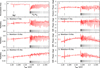 |
Fig. 1. VLTI/AMBER observations of the red giant Arcturus. Panel a: observed spectrum normalized to the continuum. The positions of the CO lines and the Mg I line are marked with the ticks. Panels b–d: visibilities observed at 7.3, 14.6, and 21.8 m, respectively. The leftmost error bars represent the typical total errors, while the smaller error bars represent the typical errors without the systematic errors resulting from the absolute calibration. Panel e: observed closure phase. The errors are shown in the same manner as in panels b–d. Panels f–h: differential phases observed at the 7.3, 14.6, and 21.8 m baselines, respectively. The errors are shown in the same manner as in panels b–d. |
2. VLTI/AMBER observations
We observed Arcturus with the near-infrared interferometric instrument AMBER (Petrov et al. 2007) at ESO’s Very Large Telescope Interferometer (VLTI). The AMBER instrument operates between 1.3 and 2.4 μm and allows us to combine three 8.2 m unit telescopes (UTs) or 1.8 m auxiliary telescopes (ATs) and achieve a spatial resolution of down to 2 mas at 2 μm with spectral resolutions of 35, 1500, and 12 000. Our AMBER observations of Arcturus took place on 2014 February 11 (UTC) using the B2-C1-D0 AT configuration, which provided projected baseline lengths of 7.3, 14.6, and 21.8 m. We observed a spectral window between 2.28 and 2.31 μm with a spectral resolution of 12 000, which is sufficient to spectrally resolve individual CO first overtone lines near the v = 2 − 0 band head located at 2.294 μm. We did not use the VLTI fringe-tracker FINITO, because Arcturus saturates FINITO. Nevertheless, the high brightness of the target enabled us to record fringes of good quality with a detector integration time (DIT) of 120 ms. The log of our observations is summarized in Table 1.
The data were reduced with amdlib ver 3.0.71. The amdlib software extracts the following observables from the recorded interferograms based on the P2VM algorithm (Tatulli et al. 2007; Chelli et al. 2009): squared visibility amplitude, closure phase (CP), and wavelength-differential phase (DP). The visibility amplitude corresponds to the amplitude of the complex Fourier transform of the object’s intensity distribution on the sky. The CP is the sum of the phases of the complex Fourier transform measured on three baselines forming a closed telescope triangle. Since the CP is zero or π for a point-symmetric object, non-zero and non-π CPs indicate asymmetry in the object. The DP represents the Fourier phase of the object on a given baseline in spectral features (e.g., atomic or molecular lines) with respect to the continuum. The DP is related to the photocenter shift of the object in spectral features with respect to the continuum.
The interferometric observables extracted with amdlib were calibrated with the observations of α Cen A (G2V), which was observed not only for the calibration of the Arcturus data, but also for other targets in the same observing program. We computed the transfer function adopting a uniform-disk diameter of 8.314 ± 0.016 mas for α Cen A (Kervella et al. 2003). The Arcturus data were calibrated with the transfer function values measured before and after Arcturus, while the errors in the interferometric observables were estimated including the standard deviation of all transfer function values measured throughout the night. The atmospheric conditions were very stable with a seeing of mostly 0″̣8–1″̣0 and coherence time (τ0) of 4–5 ms, and therefore the transfer function was stable throughout the night, as shown in Fig. A.1. This means that although the DIT is longer than the coherence time (20–30 ms at 2.3 μm, assuming τ0(λ)∝λ6/5), the effects of the atmosphere on the interferometric observables were stable, and therefore the science data can be well calibrated.
We compared the results we obtained by keeping only the best 20% and 80% of the frames in terms of the fringe signal-to-noise ratio (S/N). The results obtained with the best 20% of the frames show smaller errors in the visibilities. On the other hand, the errors in the DPs and CP are smaller if the best 80% of the frames are kept (i.e., discarding the worst 20% of the frames). Therefore, we adopted the visibilities obtained from the best 20% of the frames and the CP and DPs obtained from the best 80% of the frames. The spectrum was obtained by using the best 80% of the frames.
The total errors in the visibilities, DPs, and CP are dominated by the systematic errors resulting from the absolute calibration. We estimated the relative errors in the wavelength-differential visibilities, DPs, and CP (i.e., errors without the systematic errors due to the absolute calibration) as follows. The data of Arcturus consist of five exposures taken consecutively (see Table 1). We reduced and calibrated each exposure separately in the same manner as described above. The visibilities resulting from five exposures are normalized to 1 in the continuum. We took the standard deviation of these normalized visibilities among five exposures at each wavelength as the relative errors in the wavelength-differential visibilities. The relative errors in the wavelength-differential DPs and CP were estimated in the same manner, but without normalizing to 1.
The wavelength calibration was carried out using the telluric lines identified in the observed spectrum of α Cen A, as described in Ohnaka et al. (2009). The uncertainty in wavelength calibration is 2.1 × 10⁻⁵μm, which translates into 2.7 km s−1. The observed wavelength scale was then converted into the laboratory frame using the heliocentric velocity of −5.2 km s−1 of Arcturus (Gontscharov 2006). The spectroscopic calibration (e.g., removal of the telluric lines and instrumental effects from the observed spectrum of Arcturus) was done using the observed spectrum of α Cen A based on the procedure described in Ohnaka et al. (2013).
3. Results
Figure 1 shows the observed spectrum, visibilities, closure phase, and differential phases of Arcturus2. The high spectral resolution of the AMBER instrument enables the signatures of the individual CO lines3 to be clearly visible in the interferometric observables. It should be noted that while the changes in the visibilities observed in the CO lines may appear to be marginal compared to the error bars (the larger error bars shown in the far left in Figs. 1b–d), the errors are dominated by the systematic errors in the absolute calibration. The relative errors in the wavelength-differential visibilities are much smaller, 0.7% at the shortest and middle baselines and 1.5% at the longest baseline, as shown by the smaller error bars in the figure. This means that the signatures of the CO lines in the visibilities are real.
The drop in visibilities in the CO lines means that the star appears larger in the CO lines. This is qualitatively expected because the CO first overtone lines form in the upper photosphere and in the outer atmosphere. However, the visibilities in the CO lines near the band head (≲2.3 μm) are higher than in the continuum. This is particularly clearly visible in the data taken at the shortest baseline, as shown in Fig. 2. The figure also reveals that the visibilities in these CO lines do not simply rise above the continuum level, but are asymmetric with respect to the center of the line profile: the visibility shows a spike above the continuum level in the blue wing, while it drops below the continuum level in the red wing. As we show in Sect. 4, the visibility spikes rising above the continuum level cannot be reproduced by our models. The visibilities higher than the continuum level mean that the star appears smaller in the blue wing of the lines. A possible reason is a strong stellar spot. Similar visibilities that are asymmetric in the blue and red wing (i.e., tilde-shaped) are observed in the RSGs Betelgeuse and Antares (Ohnaka et al. 2009, 2011, 2013), and can be explained by upwelling or downdrafting large spots in the atmosphere. The inhomogeneous velocity field in the atmosphere of Antares has been imaged with VLTI/AMBER (Ohnaka et al. 2017). Therefore, Arcturus might also show such spots. Further observations, preferably aperture-synthesis imaging, is necessary to confirm this.
We fit the visibilities measured at each wavelength with a uniform disk to have an approximate idea about the increase of the star’s size in the CO lines. As Fig. 3 shows, the uniform-disk diameter in the continuum is 20.4 ± 0.2 mas, which agrees well with the previous measurements in the infrared (20.44 ± 0.16 mas at 2.22 μm, Verhoelst et al. 2005; 20.304 ± 0.011 mas at 1.65 μm, Lacour et al. 2008). The uniform-disk diameter increases up to ∼21 mas in the CO band head, and it stays at ∼20.6 mas in the individual CO lines. Although the increase in the uniform-disk diameter in the CO band head and CO lines may seem insignificant, it provides us with important information about the extended atmosphere, as we present in Sect. 4. In the CO lines near the band head, the uniform-disk diameter decreases to ∼20.2 mas, reflecting the visibility spikes described above.
The continuum visibilities observed at the 14.6 and 21.8 m baselines show a slight increase with wavelength. This is for the following reason. On the one hand, the spatial frequency decreases toward longer wavelengths (λ) for a given baseline length (B), because it is defined as B/λ. On the other hand, if the star approximately appears to be a uniform disk or limb-darkened disk in the continuum, the visibility increases toward lower spatial frequencies in the first lobe (as in the case of our observations). Therefore, the visibility in the continuum, when shown as a function of wavelength, increases toward longer wavelengths.
We also detected non-zero DPs and CP in the CO lines, which indicate asymmetry in the CO lines, perhaps due to inhomogeneities in the CO-line-forming upper layers, as mentioned above. Furthermore, a closer look at the data shows that the DPs observed at the 14.6 and 21.8 m baselines are asymmetric with respect to the center of the line profile. As Fig. 4 shows, the maxima of the DPs are located in the blue wing of the line profiles, while the minima are located in the red wing. This means that the photocenter of the object is different in the blue and red wings. In other words, the star appears differently in the blue and red wings. The DP observed on the shortest baseline of 7.3 m also shows signatures of such asymmetry across the line profile (the minima of the visibilities are slightly shifted to the blue wing), but less significant compared to two longer baselines. This asymmetry in the DPs and CPs across the CO line profiles is similar to what has been observed in the RSGs Betelgeuse and Antares (Ohnaka et al. 2009, 2011, 2013) and may also imply inhomogeneous structures, together with the asymmetry in the visibility observed at the 7.3 m baseline, as described above.
The weak line at 2.2814 μm is identified to be Mg I. The signature of this line can be seen in the observed visibilities as well as in the CP and DPs. The visibilities in the Mg I line at the shortest and longest baselines show a tilde-shaped signature: a peak in the blue wing, and a drop in the red wing of the line. The uniform-disk diameter in the Mg I line also reflects the asymmetry, as shown in Fig. 3. This is similar to the visibility spikes in the CO lines described above, and cannot be interpreted by the modeling we present here. Therefore, we refrain from modeling the Mg I line in this work.
There are also other very weak lines shortward of the CO band head. However, they are located at the wavelengths of some telluric lines, and it is possible that they are still affected by the residual of the removal of the telluric lines.
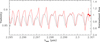 |
Fig. 2. Enlarged view of the visibility in the CO lines observed at the shortest baseline of 7.3 m (red line). It shows asymmetry with respect to the line center. The typical errors are shown in the right in the same manner as in Fig. 1. The scaled observed spectrum is shown with the black line. |
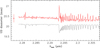 |
Fig. 3. Uniform-disk diameter of Arcturus. The typical error is shown in the left. The scaled observed spectrum is shown in black. |
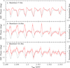 |
Fig. 4. Enlarged view of the observed differential phases across the CO line profiles. The data obtained at 7.3, 14.6, and 21.8 m are shown in panels a, b, and c, respectively. In each panel, the red line with the error bars (total errors) shows the observed differential phase, while the black line shows the observed scaled spectrum. |
4. Modeling the AMBER data
4.1. Comparison with MARCS models
We first compare the observed visibilities with the MARCS photospheric models (Gustafsson et al. 2008) to see whether the observed data in the CO lines can be explained by the photosphere without any additional component such as the MOLsphere or COmosphere. The MARCS models are plane-parallel or spherical hydrostatic photospheric models that incorporate a great number of atomic and molecular lines. The models are based on local thermodynamical equilibrium (LTE), in which convection is taken into account by means of the mixing length theory. In the spherical MARCS models, each model is specified by effective temperature (Teff), surface gravity (log g), microturbulent velocity (vmicro), stellar mass (M⋆), and chemical composition.
For the basic stellar parameters of Arcturus, we adopted Teff = 4250 ± 50 K, log g = 1.7 ± 0.1, M⋆ = 1.1 M⊙, vmicro = 2.0 km s−1, and [Fe/H] = −0.4 (Tsuji 2009; Smith et al. 2013). The CNO abundances in Arcturus roughly agree with the moderately CN-cycled chemical composition used in the MARCS model grid. Therefore, we used the MARCS model with Teff = 4250 K, log g = 1.5, M⋆ = 1.0 M⊙, vmicro =2.0 km s−1, and [Fe/H] = −0.5 with the moderately CN-cycled composition. Using the density and temperature stratifications downloaded from the MARCS model site4, we first computed the intensity profile at each wavelength and then the flux and visibility as described in Ohnaka (2013). The angular scale of the model visibilities was set so that the model visibilities computed in the continuum at three observed baselines matched the observed data within the measurement errors. The CO line opacity was calculated using the line list of Goorvitch (1994), and a Gaussian line profile was assumed. The flux and visibility were spectrally convolved to match the spectral resolution of AMBER, 12 000.
Figure 5 shows a comparison of the MARCS model and the observed data of Arcturus. While there is an offset between the observed and model visibility levels at the longest baseline of 21.8 m, this is within the uncertainty of the absolute visibility calibration. The model can clearly reproduce the observed spectrum very well. However, the visibilities predicted by the model show too shallow decreases in the CO lines except for the 21.8 m baseline. This means that the atmosphere of Arcturus is more extended than the MARCS model predicts, or there is an extended component above the photosphere that is not accounted for by the MARCS model.
We also computed the synthetic spectrum and visibilities using the MARCS model with a higher turbulent velocity of 5 km s−1 instead of 2 km s−1 (the other model parameters were the same). The model with 5 km s−1 predicts the CO absorption lines to be slightly stronger (therefore, the agreement with the observed spectrum is slightly worse). The predicted visibilities are nearly the same as those predicted by the model with 2 km s−1 : the model visibilities in the CO lines are still too high compared to the observed data. The geometrical extension of these MARCS photospheric models is only ∼2%, which is insufficient by far to explain the observed visibilities. Our result is qualitatively consistent with the finding of Tsuji (2009) that the strong CO first overtone lines in Arcturus cannot be explained by current photospheric models and show the presence of the additional extended component MOLsphere. In other words, our AMBER observations have spatially resolved the MOLsphere of Arcturus in the individual CO lines.
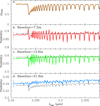 |
Fig. 5. Comparison of the observed visibilities of Arcturus with those predicted by the MARCS photospheric model. Panel a shows a comparison of the spectrum, while panels b–d show a comparison of the visibilities observed at the 7.3, 14.6, and 21.8 m baselines, respectively. In each panel, the thick solid line represents the observed data, and the thin solid line represents the model. The typical errors are shown in the same manner as in Fig. 1. The parameters of the MARCS model are described in Sect. 4.1. |
The result that the MARCS model cannot explain the visibilities observed in the individual CO first overtone lines of normal (i.e., non-Mira-type) K–M giants has been reported for the K5 giant Aldebaran and M7 giant BK Vir (Ohnaka 2013; Ohnaka et al. 2012), which are cooler than Arcturus. However, Arroyo-Torres et al. (2014) found no signatures of a non-photospheric component in the visibilities obtained across the CO bands at 2.3–2.45 μm in four out of five red giants from G8III to M6III. Only in the M2III star β Peg did they find signatures of a non-photospheric extended component. However, their negative detection may be due to the lower spectral resolution of 1500 compared to the 12 000 used in our observations. To see whether the signatures of the CO lines in the visibilities observed in Arcturus can still be detected with the spectral resolution of 1500, we spectrally binned the raw data (object, dark, sky, and P2VM calibration data) to a resolution of 1600 with a running box-car function as described in Ohnaka et al. (2009). The binned data were reduced and calibrated in the same manner as the original unbinned data. Figure 6 illustrates that while the spectrum still shows the CO band head, the visibilities show no signatures of the CO band when binned down to 1600. Therefore, high spectral resolution is essential to confirm the presence or absence of the MOLsphere in normal K–M giants.
In contrast to the MOLsphere of normal (non-Mira-type) K–M giants, the AMBER observations of a sample of RSGs carried out by Arroyo-Torres et al. (2015) and Wittkowski et al. (2017) show the presence of the MOLsphere, although the same spectral resolution of 1500 was used. Arroyo-Torres et al. (2015) showed that the visibilities in the CO bands observed in their RSGs significantly deviate from what is predicted by the photospheric models, which is the signature of the presence of the MOLsphere. On the other hand, most of the red giants in their sample do not show the signature of the MOLsphere (see their Fig. 10). Therefore, it is suggested that the emission from the MOLsphere in RSGs is stronger than in normal K–M giants, possibly because the density and/or temperature of the MOLsphere is higher and/or the MOLsphere is more extended.
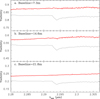 |
Fig. 6. Visibilities of Arcturus obtained at a spectral resolution of 1600. The visibilities at the 7.3, 14.6, and 21.8 m baselines are plotted with thick red lines in panels a, b, and c, respectively. In each panel, the black line shows the scaled spectrum. |
4.2. Comparison with MARCS+MOLsphere models
As described in Sect. 1, the dust-driven stellar wind models and pulsation-driven wind models are probably not appropriate for Arcturus. No Alfvén-wave-driven models currently take the thermal structure and dynamics of the weakly ionized outer atmosphere of red giants into account in a self-consistent manner. In other words, it is not clear yet which physical process is responsible for the formation of the MOLsphere.
Parameters of the MARCS+MOLsphere models for Arcturus and the best-fit solution.
Therefore, to characterize the extended MOLsphere component detected in our AMBER observations, we used the semi-empirical model that has been applied to derive the parameters of the MOLsphere in our previous studies (Ohnaka et al. 2012; Ohnaka 2013). In this model, one or two layers are added above the MARCS photospheric models. Each layer is defined by its inner and outer radius and assumed to have a constant temperature and density. We adopted the photospheric microturbulent velocity of 2 km s−1 for these layers. We first attempted to explain the observed data with the MARCS+1-layer models. However, it turned out to be impossible to obtain a satisfactory fit to the visibilities measured on all three baselines. Therefore, we carried out the modeling with two layers. The ranges of the parameters are listed in Table 2, together with the best-fit solution. We note that when computing the model grid, the radius of the inner layer was always set to be equal to or larger than the uppermost layer of the MARCS model, which is located at 1.02 R⋆. The uncertainties in the parameters of the best-fit model were estimated by varying them around the best-fit solution.
The geometrical thickness of the layers was not well constrained in our previous studies, and therefore was assumed to be 0.1 R⋆. However, in the case of Arcturus, the models with this assumption did not reproduce the observed data even with two layers. Therefore, we changed the thickness of the layers as well. We found that it is necessary to reduce the thickness of the inner layer at least to 0.02 R⋆ to obtain a reasonable fit to the data. Models with thicknesses of between 0.01 and 0.02 R⋆ can reproduce the data equally well, which means that we cannot further constrain the thickness of the inner layer. On the other hand, the thickness of the outer layer is not well constrained, and the adoption of 0.1 R⋆ resulted in reasonable agreement with the data.
Figure 7 shows a comparison between the best-fit model and the observed data. The observed visibilities in the CO lines are much better reproduced than with the MARCS-only model presented in Sect. 4.1. The agreement with the observed spectrum is also reasonable. The visibility decrease observed in the CO lines at the shortest baseline of 7.3 m suggests the presence of a very extended component. This is why our modeling shows that the outer layer extends out to 2.6 R⋆. The inner layer is dense and is located very close to the star, at 1.04 R⋆. The presence of this dense compact layer is needed to explain the observed data for the following reason. If the object only consists of the photosphere and the outer CO layer, the visibility predicted in the CO lines at the longest baseline is significantly lower than that observed, owing to the extended outer CO layer. The emission from the dense inner CO layer just above the photosphere causes the object to appear more compact, canceling the effect described above due to the outer CO layer.
We estimated the gas density in the MOLsphere CO layers as follows. We can convert the derived CO column density into the CO number density by dividing by the geometrical thickness of the layer. While we assumed two distinct layers to simplify the models, the actual density distribution of the MOLsphere can be continuous. Therefore, we took (Rinner (outer) − R⋆) as an upper limit on the geometrical thickness of the CO layer. The CO number densities derived for the inner and outer CO layers are 1.2 × 10⁹ and 3.1 × 106 cm−3, respectively. These values are lower limits of the CO number densities. Then assuming chemical equilibrium at the temperature derived for each CO layer, we estimated the H2, H, and He number densities so that the CO number density is reproduced. The gas density, which can be computed from the derived H2, H, and He number densities, is 1.5 × 10⁻¹¹ and 3.7 × 10⁻¹⁴ g cm−3 for the inner and outer CO layer, respectively.
It may appear to be puzzling that the spectrum predicted by the MARCS+MOLsphere model is nearly the same as that from the MARCS-only model. This can be explained as follows. The spectrum from the extended MOLsphere beyond the limb of the star shows the CO lines in emission. However, the spectrum inside the limb shows additional absorption in the CO lines, because we see the cooler MOLsphere in front of the warmer star. In the total spectrum, which is the spatial sum of these emission and absorption spectra, the signatures of the MOLsphere can disappear, as illustrated in Ohnaka (2013, Sect. 4).
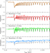 |
Fig. 7. Comparison of the observed visibilities of Arcturus with those predicted by the MARCS+MOLsphere model, shown in the same manner as in Fig. 5. The model parameters are described in Sect. 4.2 and listed in Table 2. |
Ryde et al. (2002) detected H2O lines near 12 μm in Arcturus, which is a surprise because the photosphere of Arcturus is deemed to be too hot for H2O to form. Ryde et al. (2002) argued that the H2O lines originate from the uppermost photospheric layers. They showed that the observed H2O lines can be explained without introducing a non-photospheric component such as the MOLsphere if the temperature of the uppermost photospheric layers is decreased by ∼300 K. While this scenario for the formation of H2O may still be viable, it does not disprove the presence of the MOLsphere either, because it is now spatially resolved with our VLTI/AMBER observations.
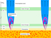 |
Fig. 8. Schematic view of the thermally and dynamically inhomogeneous outer atmosphere of Arcturus. The structure of the chromospheric region is based on Fig. 6 of Ayres et al. (2003). The authors postulated that closed magnetic loops (shown in violet), which are responsible for the hot coronal gas, are submerged in the chromospheric gas at lower temperatures (shown in blue). The locations of the two CO layers are based on our modeling. While we adopted two discrete CO layers in our modeling, it is possible that the actual density distribution of this cool molecular component is continuous. This is represented by the pale green region between the inner and outer CO layers as well as between the photosphere and the inner CO layer. |
5. Discussion
The analysis of the spectra of the CO fundamental lines of a sample of red giant stars, including Arcturus, by Wiedemann et al. (1994) suggests a monotonic decrease in temperature above the temperature minimum predicted by the chromospheric models. The authors estimated temperatures of 2000–3000 K in the same atmospheric heights where the chromospheric model predicts the temperature to increase up to ∼6000 K. The temperatures of the cool component are in broad agreement with the temperatures of the MOLsphere derived from our modeling, given the differences in the observed data as well as in the photospheric models.
Tsuji (2009) estimated the temperature and CO column density of the MOLsphere of Arcturus to be 2000 K and 5 × 1019 cm−2, respectively, based on the spectrum of the strong CO fundamental lines. These values agree with the results that we obtained for the inner layer, 1600 ± 400 K and (0.5 − 2.0)×1020 cm−2, given the uncertainties in both models. Tsuji (2009) assumed the inner and outer radius of the MOLsphere to be 1.04 and 1.11 R⋆, respectively, which also agrees fairly well with the inner radius of 1.04 R⋆ that we derived for the inner CO layer. The modeling of Tsuji (2009) does not include a second, more extended layer, because he considered a model with as few free parameters as possible to explain the spatially unresolved spectra (albeit of much higher spectral resolution) of the CO fundamental lines.
Based on the tentative detection of X-ray emission from Arcturus and the analysis of UV emission lines, Ayres et al. (2003) postulated that the hot coronal gas with temperatures of a few 105 K associated with closed magnetic loops is submerged (“buried alive”, as the authors expressed it) in the chromosphere with a temperature below ∼104 K. Furthermore, they concluded that there should be a cool molecular layer below the chromosphere. Figure 6 of Ayres et al. (2003) shows a cool molecular layer, which is presented as COmosphere in their figure, very close to the star, within ∼1.05 R⋆. This agrees with the radius of the inner CO layer of our model. They also pointed out the possible presence of inhomogeneous structures, such as holes in the chromosphere, to explain the observed fluorescence spectra of CO and H2. This is qualitatively consistent with the conclusion from the analysis of the infrared CO lines by Wiedemann et al. (1994) and Tsuji (2009). The detection of non-zero CP and DPs presented in Sect. 2 lends direct support to the presence of inhomogeneous structures. It should be noted that while the inner CO layer of our models is consistent with the previous studies, our AMBER observations and modeling have revealed that the cool molecular component extends out to 2–3 R⋆, much farther than considered before.
The chromospheric model of Drake (1985) for Arcturus based on the analysis of UV emission lines shows that the (electron) temperature already reaches ∼8000 K at ∼1.2 R⋆ and stays approximately constant up to ∼20 R⋆. O’Gorman et al. (2013) proposed a modified model, in which the electron temperature decreases beyond 2.3 R⋆, to reproduce the radio fluxes measured at 3–20 cm. In either case, the chromospheric wind reaches the terminal velocities of 35–40 km s−1 already within ∼2 R⋆. On the other hand, our modeling of the AMBER data shows that the MOLsphere extends to ∼2.6 R⋆. This means that the chromospheric wind accelerates within the radius of the MOLsphere. Nevertheless, neither the spectrum of the CO first overtone lines nor the visibilities obtained with AMBER show a signature of this outflow in the MOLsphere, which would have been detectable with the spectral resolution of 25 km s−1 of AMBER. The analyses of the high-resolution spectra of the CO fundamental lines do not show a systematic outflow either (Heasley et al. 1978; Wiedemann et al. 1994; Tsuji 2009). Tsuji (1988) inferred that the MOLsphere is quasi-static, because even if it does not show a systematic outflow, it is characterized by strong turbulence with a turbulent velocity as high as 10 km s−1.
Our AMBER observations and modeling of Arcturus, combined with the analysis of the chromospheric emission lines, suggest the coexistence of two components within 2–3 R⋆ that are distinct not only thermally, but also dynamically: a quasi-static cool molecular component, and a steeply accelerating chromospheric wind.
Figure 8 shows a schematic view of the inhomogeneous structures of the outer atmosphere of Arcturus. The stratification in the chromospheric region is taken from Fig. 6 of Ayres et al. (2003). While their figure shows the chromosphere only up to 1.15 R⋆, we assumed it to extend to much larger radii to represent the chromospheric wind. The cool molecular component, which covers most of the surface of the star, extends to the same atmospheric heights as the chromospheric component (at least to ∼2.6 R⋆). It should be kept in mind that the geometrical thickness of the outer CO layer was assumed to be 0.1 R⋆ in our modeling, because it cannot be constrained by the current data. It is possible or rather realistic that the outer layer is geometrically thicker with a continuous density distribution. Observations with higher spatial resolution are necessary to probe this issue.
The physical process responsible for the formation of the outer atmosphere consisting of the hot chromospheric gas and cool molecular gas is not yet understood. As discussed in Ohnaka (2013), the Alfvén-wave-driven wind models (Suzuki 2007) show highly temporally variable stellar winds consisting of hot gas (104 − 105 K) embedded in cool gas (1000–2000 K). The temperatures of this cool component are in agreement with the results of our modeling. Since the models assume fully ionized plasma, which is not appropriate for the outer atmosphere of red giants, it is necessary to compare with the observations once the models are further improved.
The recent 3D simulations of the chromosphere of red giants by Wedemeyer et al. (2017) show that the shock waves produced by convective motions give rise to filaments of hot gas reaching a temperature of ∼5000 K, even when magnetic fields are not included. The filamentary chromospheric gas is embedded in cooler gas at a temperature as low as ∼2000 K within an atmospheric height of ∼2 × 1011 cm, which corresponds to ∼1.1 R⋆ for the stellar radius of 2.05 × 1012 cm predicted by the MARCS models for Arcturus. The temperature and the atmospheric height of this cool gas are comparable to the temperatures and radius of the inner CO layer derived from our modeling. The models of Wedemeyer et al. (2017) also show that the density of the cool gas at atmospheric heights within ≲1011 cm (≲1.05 R⋆) is as high as ∼10−11 g cm−3, which broadly agrees with the gas density of 1.5 × 10⁻¹¹ g cm−3 of the inner CO layer derived in Sect. 4.2. While the geometrical extension of the 3D models is still too small compared to the overall extension of the MOLsphere of 2–3 R⋆, it would be interesting to compare such theoretical models with the observationally derived properties of the MOLsphere, once they are extended to larger radii.
As described in Sect. 4.1, RSGs tend to show more pronounced emission from the MOLsphere than normal K–M giants. Based on high spectral resolution AMBER data, we have derived the parameters of the MOLsphere for two RSGs (Betelgeuse and Antares, Ohnaka et al. 2009, 2011, 2013) and three normal K–M giants (BK Vir, Aldebaran, and Arcturus, Ohnaka et al. 2012; Ohnaka 2013, and this work). However, the differences in the effective temperature between two RSGs and three red giants do not allow us to discuss possible differences in the MOLsphere parameters between RSGs and normal K–M giants. We have carried out high spectral resolution AMBER observations for a small sample (about ten stars) of red giants and RSGs to study the possible systematic dependence of the MOLsphere properties on basic stellar parameters such as luminosity, effective temperature, and surface gravity. The results will be reported in a future paper.
6. Concluding remarks
Our high spectral resolution infrared interferometric observations of the well-studied red giant Arcturus in the individual 2.3 μm CO lines have spatially resolved the molecular outer atmosphere. The MARCS photospheric models are too compact to explain the observed data in the CO lines, confirming that the extended molecular outer atmosphere is not accounted for by current photospheric models. The observed spectra and visibilities can be reproduced by models in which two additional CO layers are added above the MARCS photospheric model. The inner CO layer is geometrically thin (≲0.02 R⋆) and is located just above the photosphere, at 1.04 ± 0.02 R⋆, with a CO column density of 1020 ± 0.3 cm−2 and a temperature of 1600 ± 400 K. The properties of this layer are in agreement with what has been inferred from previous spatially unresolved spectroscopic studies in the infrared and ultraviolet. The outer CO layer, however, extends out to 2.6 ± 0.2 R⋆, which is much larger than considered before, with a CO column density of 1019 ± 0.15 cm−2 and a temperature of 1800 ± 100 K.
Combined with the chromospheric models that are based on the UV emission lines, our AMBER observations and modeling suggest that the quasi-static cool molecular component extends out to 2–3 R⋆, within which the chromospheric wind steeply accelerates. The detection of the non-zero CP and DPs also suggests the presence of such inhomogeneous structures. It is not clear yet whether the cool component remains quasi-static beyond 2–3 R⋆ or starts to exhibit a systematic outflow at some radius. Moreover, it is not clear either to what radius the cool molecular component extends, because the CO first overtone lines sample a relatively warm region. Spatially resolved observations in the CO fundamental lines would be useful to probe the region farther out and obtain a more comprehensive picture of the outer atmosphere. This will be possible with the second-generation VLTI instrument MATISSE (Lopez et al. 2014).
Strictly speaking, taking the square root of the squared visibility amplitude extracted with amdlib makes the errors asymmetric. However, this effect is very small in our case, and the errors in the visibility amplitude are still nearly symmetric. We show the visibility amplitude to facilitate a comparison with our previous results.
These spectral features that appear to be single lines consist of two CO transitions with high J and low J, where J is the rotational quantum number.
Acknowledgments
We thank the ESO Paranal team for supporting our AMBER observations. We are also grateful to Dieter Schertl and Karl-Heinz Hofmann for their help with the AMBER data reduction. K. O. acknowledges the support of the Comisión Nacional de Investigación Científica y Tecnológica (CONICYT) through the FONDECYT Regular grant 1180066. This research made use of the SIMBAD database, operated at the CDS, Strasbourg, France, and NSO/Kitt Peak FTS data on the Earth’s telluric features produced by NSF/NOAO.
References
- Airapetian, V. S., Carpenter, K. G., & Ofman, L. 2010, ApJ, 723, 1210 [NASA ADS] [CrossRef] [Google Scholar]
- Arroyo-Torres, B., Martí-Vidal, I., Marcaide, J. M., et al. 2014, A&A, 566, A88 [NASA ADS] [CrossRef] [EDP Sciences] [Google Scholar]
- Arroyo-Torres, B., Wittkowski, M., Chiavassa, A., et al. 2015, A&A, 575, A50 [NASA ADS] [CrossRef] [EDP Sciences] [Google Scholar]
- Ayres, T. R., & Linsky, J. L. 1975, ApJ, 200, 660 [NASA ADS] [CrossRef] [Google Scholar]
- Ayres, T. R., Brown, A., & Harper, G. M. 2003, ApJ, 598, 610 [NASA ADS] [CrossRef] [Google Scholar]
- Bedding, T. R. 2000, in The Third MONS Workshop: Science Preparation and Target Selection, eds. T. C. Teixeira, & T. R. Bedding (Aarhus Universitet), 97 [Google Scholar]
- Chelli, A., Hernandez Utrera, O., & Duvert, G. 2009, A&A, 502, 705 [NASA ADS] [CrossRef] [EDP Sciences] [Google Scholar]
- Cranmer, S., & Saar, S. H. 2011, ApJ, 741, 54 [NASA ADS] [CrossRef] [Google Scholar]
- Drake, S. A. 1985, Progress in Stellar Spectral Line Formation Theory, eds. J. E.Beckman, & L. Crivellari(Dordrecht: Reidel), Proc. Advanced Research Workshop, 351, [Google Scholar]
- Goorvitch, D. 1994, ApJS, 95, 535 [NASA ADS] [CrossRef] [Google Scholar]
- Gontscharov, G. A. 2006, Astron. Lett., 32, 759 [NASA ADS] [CrossRef] [Google Scholar]
- Gustafsson, B., Edvardsson, B., Eriksson, K., et al. 2008, A&A, 486, 951 [NASA ADS] [CrossRef] [EDP Sciences] [Google Scholar]
- Heasley, J. N., Ridgway, S. T., Carbon, D. F., Milkey, R. W., & Hall, D. N. B. 1978, ApJ, 219, 970 [NASA ADS] [CrossRef] [Google Scholar]
- Hillen, M., Verhoelst, T., Degroote, P., Acke, B., & van Winckel, H. 2012, A&A, 538, L6 [NASA ADS] [CrossRef] [EDP Sciences] [Google Scholar]
- Hinkle, K. H. 1978, ApJ, 220, 210 [NASA ADS] [CrossRef] [Google Scholar]
- Höfner, S., & Olofsson, H. 2018, A&ARv, 26, 1 [NASA ADS] [CrossRef] [Google Scholar]
- Kervella, P., Thévenin, F., Ségransan, D., et al. 2003, A&A, 404, 1087 [NASA ADS] [CrossRef] [EDP Sciences] [Google Scholar]
- Lacour, S., Meimon, S., Thiébaut, E., et al. 2008, A&A, 485, 561 [NASA ADS] [CrossRef] [EDP Sciences] [Google Scholar]
- Lopez, B., Lagarde, S., Jaffe, W., et al. 2014, The Messenger, 157, 5 [NASA ADS] [Google Scholar]
- Martí-Vidal, I., Marcaide, J. M., Quirrenbach, A., et al. 2011, A&A, 529, A115 [NASA ADS] [CrossRef] [EDP Sciences] [Google Scholar]
- O’Gorman, E., Harper, G. M., Brown, A., Drake, S., & Richards, A. M. S. 2013, AJ, 146, 98 [NASA ADS] [CrossRef] [Google Scholar]
- Ohnaka, K. 2013, A&A, 553, A3 [NASA ADS] [CrossRef] [EDP Sciences] [Google Scholar]
- Ohnaka, K., Hofmann, K.-H., Benisty, M., et al. 2009, A&A, 503, 183 [NASA ADS] [CrossRef] [EDP Sciences] [Google Scholar]
- Ohnaka, K., Weigelt, G., Millour, F., et al. 2011, A&A, 529, A163 [NASA ADS] [CrossRef] [EDP Sciences] [Google Scholar]
- Ohnaka, K., Hofmann, K.-H., Schertl, D., et al. 2012, A&A, 537, A53 [NASA ADS] [CrossRef] [EDP Sciences] [Google Scholar]
- Ohnaka, K., Hofmann, K.-H., Schertl, D., et al. 2013, A&A, 555, A24 [NASA ADS] [CrossRef] [EDP Sciences] [Google Scholar]
- Ohnaka, K., Weigelt, G., & Hofmann, K-.H. 2017, Nature, 548, 310 [NASA ADS] [CrossRef] [Google Scholar]
- Petrov, R. G., Malbet, F., Weigelt, G., et al. 2007, A&A, 464, 1 [NASA ADS] [CrossRef] [EDP Sciences] [Google Scholar]
- Ryde, N., Lambert, D. L., Richter, M. J., & Lacy, J. H. 2002, ApJ, 580, 447 [NASA ADS] [CrossRef] [Google Scholar]
- Schröder, K.-P., & Cuntz, M. 2007, A&A, 465, 593 [NASA ADS] [CrossRef] [EDP Sciences] [Google Scholar]
- Sennhauser, C., & Berdyugina, S. V. 2011, A&A, 529, A100 [NASA ADS] [CrossRef] [EDP Sciences] [Google Scholar]
- Smith, V. V., Cunha, K., Shetrone, M. D., et al. 2013, ApJ, 765, 16 [NASA ADS] [CrossRef] [Google Scholar]
- Suzuki, T. K. 2007, ApJ, 659, 1592 [NASA ADS] [CrossRef] [Google Scholar]
- Tatulli, E., Millour, F., Chelli, A., et al. 2007, A&A, 464, 29 [NASA ADS] [CrossRef] [EDP Sciences] [Google Scholar]
- Tsuji, T. 1988, A&A, 197, 185 [NASA ADS] [Google Scholar]
- Tsuji, T. 2000a, ApJ, 538, 801 [NASA ADS] [CrossRef] [Google Scholar]
- Tsuji, T. 2000b, ApJ, 540, L99 [NASA ADS] [CrossRef] [Google Scholar]
- Tsuji, T. 2001, A&A, 376, L1 [NASA ADS] [CrossRef] [EDP Sciences] [Google Scholar]
- Tsuji, T. 2009, A&A, 504, 543 [NASA ADS] [CrossRef] [EDP Sciences] [Google Scholar]
- Tsuji, T., Ohnaka, K., Aoki, W., & Yamamura, I. 1997, A&A, 320, L1 [NASA ADS] [Google Scholar]
- van Leeuwen, F. 2007, A&A, 474, 653 [NASA ADS] [CrossRef] [EDP Sciences] [Google Scholar]
- Verhoelst, T., Bordé, P. J., Perrin, G., et al. 2005, A&A, 435, 289 [NASA ADS] [CrossRef] [EDP Sciences] [Google Scholar]
- Wang, Y.-M. 1998, ASP Conf. Ser., 154, 131 [NASA ADS] [Google Scholar]
- Wedemeyer, S., Kučinskas, A., Klevas, J., & Ludwig, H.-L. 2017, A&A, 606, A26 [NASA ADS] [CrossRef] [EDP Sciences] [Google Scholar]
- Wiedemann, G., Ayres, T. R., & Saar, S. H. 1994, ApJ, 423, 806 [NASA ADS] [CrossRef] [Google Scholar]
- Wittkowski, M., Boboltz, D. A., Driebe, T., et al. 2008, A&A, 479, L21 [NASA ADS] [CrossRef] [EDP Sciences] [Google Scholar]
- Wittkowski, M., Boboltz, D. A., Ireland, M., et al. 2011, A&A, 532, L7 [NASA ADS] [CrossRef] [EDP Sciences] [Google Scholar]
- Wittkowski, M., Chiavassa, A., Freytag, B., et al. 2016, A&A, 587, A12 [NASA ADS] [CrossRef] [EDP Sciences] [Google Scholar]
- Wittkowski, M., Arroyo-Torres, B., Marcaide, J. M., et al. 2017, A&A, 597, A9 [NASA ADS] [CrossRef] [EDP Sciences] [Google Scholar]
- Woodruff, H. C., Ireland, M. J., Tuthill, P. G., et al. 2009, ApJ, 691, 1328 [NASA ADS] [CrossRef] [Google Scholar]
Appendix A: Transfer function of the AMBER observations
Figure A.1 shows the transfer function (i.e., the visibility that would be measured for a point source) derived from the AMBER observations of the calibrator α Cen A. It was derived by taking the best 20% of the frames in terms of the fringe S/N and used for the calibration of the Arcturus data. The figure shows that the transfer function values on three baselines are very stable throughout the night, thanks to the good and stable atmospheric conditions.
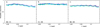 |
Fig. A.1. Transfer function derived on the night of the observation of Arcturus. Panels a, b, and c show the transfer function measured at baselines B2–C1, C1–D0, and B2–D0, respectively, taking the best 20% of the frames in terms of the fringe S/N. In each panel, the transfer functions derived from five AMBER observations of the calibrator α Cen A (C1–C5 in Table 1) are plotted in black (C1), red (C2), green (C3), blue (C4), and light blue (C5). The transfer function was stable throughout the night, and the five curves therefore nearly overlap. |
All Tables
Parameters of the MARCS+MOLsphere models for Arcturus and the best-fit solution.
All Figures
|
Fig. 1. VLTI/AMBER observations of the red giant Arcturus. Panel a: observed spectrum normalized to the continuum. The positions of the CO lines and the Mg I line are marked with the ticks. Panels b–d: visibilities observed at 7.3, 14.6, and 21.8 m, respectively. The leftmost error bars represent the typical total errors, while the smaller error bars represent the typical errors without the systematic errors resulting from the absolute calibration. Panel e: observed closure phase. The errors are shown in the same manner as in panels b–d. Panels f–h: differential phases observed at the 7.3, 14.6, and 21.8 m baselines, respectively. The errors are shown in the same manner as in panels b–d. |
| In the text | |
|
Fig. 2. Enlarged view of the visibility in the CO lines observed at the shortest baseline of 7.3 m (red line). It shows asymmetry with respect to the line center. The typical errors are shown in the right in the same manner as in Fig. 1. The scaled observed spectrum is shown with the black line. |
| In the text | |
|
Fig. 3. Uniform-disk diameter of Arcturus. The typical error is shown in the left. The scaled observed spectrum is shown in black. |
| In the text | |
|
Fig. 4. Enlarged view of the observed differential phases across the CO line profiles. The data obtained at 7.3, 14.6, and 21.8 m are shown in panels a, b, and c, respectively. In each panel, the red line with the error bars (total errors) shows the observed differential phase, while the black line shows the observed scaled spectrum. |
| In the text | |
|
Fig. 5. Comparison of the observed visibilities of Arcturus with those predicted by the MARCS photospheric model. Panel a shows a comparison of the spectrum, while panels b–d show a comparison of the visibilities observed at the 7.3, 14.6, and 21.8 m baselines, respectively. In each panel, the thick solid line represents the observed data, and the thin solid line represents the model. The typical errors are shown in the same manner as in Fig. 1. The parameters of the MARCS model are described in Sect. 4.1. |
| In the text | |
|
Fig. 6. Visibilities of Arcturus obtained at a spectral resolution of 1600. The visibilities at the 7.3, 14.6, and 21.8 m baselines are plotted with thick red lines in panels a, b, and c, respectively. In each panel, the black line shows the scaled spectrum. |
| In the text | |
|
Fig. 7. Comparison of the observed visibilities of Arcturus with those predicted by the MARCS+MOLsphere model, shown in the same manner as in Fig. 5. The model parameters are described in Sect. 4.2 and listed in Table 2. |
| In the text | |
|
Fig. 8. Schematic view of the thermally and dynamically inhomogeneous outer atmosphere of Arcturus. The structure of the chromospheric region is based on Fig. 6 of Ayres et al. (2003). The authors postulated that closed magnetic loops (shown in violet), which are responsible for the hot coronal gas, are submerged in the chromospheric gas at lower temperatures (shown in blue). The locations of the two CO layers are based on our modeling. While we adopted two discrete CO layers in our modeling, it is possible that the actual density distribution of this cool molecular component is continuous. This is represented by the pale green region between the inner and outer CO layers as well as between the photosphere and the inner CO layer. |
| In the text | |
|
Fig. A.1. Transfer function derived on the night of the observation of Arcturus. Panels a, b, and c show the transfer function measured at baselines B2–C1, C1–D0, and B2–D0, respectively, taking the best 20% of the frames in terms of the fringe S/N. In each panel, the transfer functions derived from five AMBER observations of the calibrator α Cen A (C1–C5 in Table 1) are plotted in black (C1), red (C2), green (C3), blue (C4), and light blue (C5). The transfer function was stable throughout the night, and the five curves therefore nearly overlap. |
| In the text | |
Current usage metrics show cumulative count of Article Views (full-text article views including HTML views, PDF and ePub downloads, according to the available data) and Abstracts Views on Vision4Press platform.
Data correspond to usage on the plateform after 2015. The current usage metrics is available 48-96 hours after online publication and is updated daily on week days.
Initial download of the metrics may take a while.