| Issue |
A&A
Volume 625, May 2019
|
|
|---|---|---|
| Article Number | A24 | |
| Number of page(s) | 16 | |
| Section | Interstellar and circumstellar matter | |
| DOI | https://doi.org/10.1051/0004-6361/201833429 | |
| Published online | 03 May 2019 | |
Modeling of interactions between supernovae ejecta and aspherical circumstellar environments
1
Department of Theoretical Physics and Astrophysics, Masaryk University,
Kotlářská 2,
611,37
Brno,
Czech Republic
e-mail: petrk@physics.muni.cz
2
Institute of Theoretical Physics, Charles University,
V Holešovičkách 2,
180 00
Praha 8,
Czech Republic
Received:
15
May
2018
Accepted:
24
March
2019
Context. Massive stars are characterized by a significant loss of mass either via (nearly) spherically symmetric stellar winds or pre-explosion pulses, or by aspherical forms of circumstellar matter (CSM) such as bipolar lobes or outflowing circumstellar equatorial disks. Since a significant fraction of most massive stars end their lives by a core collapse, supernovae (SNe) are always located inside large circumstellar envelopes created by their progenitors.
Aims. We study the dynamics and thermal effects of collision between expanding ejecta of SNe and CSM that may be formed during, for example, a sgB[e] star phase, a luminous blue variable phase, around PopIII stars, or by various forms of accretion.
Methods. For time-dependent hydrodynamic modeling we used our own grid-based Eulerian multidimensional hydrodynamic code built with a finite volumes method. The code is based on a directionally unsplit Roe’s method that is highly efficient for calculations of shocks and physical flows with large discontinuities.
Results. We simulate a SNe explosion as a spherically symmetric blast wave. The initial geometry of the disks corresponds to a density structure of a material that orbits in Keplerian trajectories. We examine the behavior of basic hydrodynamic characteristics, i.e., the density, pressure, velocity of expansion, and temperature structure in the interaction zone under various geometrical configurations and various initial densities of CSM. We calculate the evolution of the SN–CSM system and the rate of aspherical deceleration as well as the degree of anisotropy in density, pressure, and temperature distribution.
Conclusions. Our simulations reveal significant asphericity of the expanding envelope above all in the case of dense equatorial disks. Our “low density” model however also shows significant asphericity in the case of the disk mass-loss rate Ṁcsd = 10−6 M⊙ yr−1. The models also show the zones of overdensity in the SN–disk contact region and indicate the development of Kelvin-Helmholtz instabilities within the zones of shear between the disk and the more freely expanding material outside the disk.
Key words: supernovae: general / stars: mass-loss / circumstellar matter / stars: evolution / hydrodynamics
© ESO 2019
1 Introduction
Explosions of supernovae (SNe) are one of the most prominent events in the universe. They may provide excellent observational and theoretical material for studying a vast range of physics: from cosmological principles to particle physics. The interaction of the SN blast wave may serve as a probe of the progenitor mass loss and its circumstellar matter (CSM).
Most of the core-collapse (type II) SN progenitors are considered to be red supergiants (Smartt 2009, 2015; Pejcha & Prieto 2015; Müller et al. 2017), however, there is strong evidence that blue supergiants (BSG) can also be hydrogen-rich massive progenitors of type II SN events (e.g., Vanbeveren et al. 2013). Most famous example is SN 1987A, which in the time of explosion was a BSG star evolved from the previous stage of red supergiant; see, for example, Meynet et al. (2015). Furthermore, there are indications of a strong connection between BSG progenitors and superluminous SNe that are likely associated with very massive stars that retained their thick hydrogen envelopes and that explode within the dense CSM environment. There is also a strong evidence of rugged and anisotropic nature of the CSM, since some of these stars may have been similar to luminous blue variables that lost a large amount of mass, up to several M⊙, prior to explosion (Smith et al. 2007, 2008; Ofek et al. 2013; Smith 2017).
The interaction of SNe with CSM may significantly power and modify the observed luminosity. After a radiation mediated shock goes through the stellar body of a SN progenitor, then it continues propagating through CSM. Depending on the optical thickness of CSM in the direction to the observer, the radiation is in the first phase more or less absorbed while an increasing amount of energy is accumulated in the shocked region (Svirski et al. 2012). After the optical depth of CSM drops, this energy is released as a breakout pulse that is much more energetic than a CSM-less breakout, however, the energy release in the presence of CSM happens over much longer timescales. Yet the energy behind the shock grows, if the CSM density does not fall abruptly, after this breakout, which is accompanied by the characteristic profile of the light curve (e.g., Chevalier & Irwin 2011; Svirski et al. 2012; Smith 2017).
It follows from the nature of (some) BSG stars that during their pre-explosion epochs a CSM may be formed that is anisotropic. In order to make a simulation of a hydrodynamic interaction of exploding SN progenitor with such aspherical CSM consisting of isotropic stellar wind component and a circumstellar equatorial disk, we consider some typical representatives of relevant types of SN progenitors that may be associated with BSG stars and with various types of circumstellar disks, such as Pop III stars, sgB[e] stars and luminous blue variables (Lee et al. 1991; Krtička et al. 2011; Kurfürst et al. 2014). We regard the structure of circumstellar disks for the purpose of modeling as that corresponding to viscous outflowing disks, which are typical for classical Be stars. However, we may assume to find this disk type in sgB[e] stars as well (for a review see, e.g., Zickgraf 1998; Hillier 2006), where a disk or rings of high density material have been detected (Kraus et al. 2013). Other types of dense equatorial disks or disk-like density enhancements may also be formed owing to, for example, magnetically compressed winds or binarity and accretion around certain classes of, for instance, B[e] stars (e.g., Hillier 2006), luminous blue variables (e.g., Schulte-Ladbeck et al. 1994; Davies et al. 2005), and post-AGB stars (e.g., Heger & Langer 1998).
Although there have been a number of studies regarding interactions of SNe expansion with various forms of spherically symmetric CSM, there is a lack of multidimensional hydrodynamic models that describe SNe interaction with dense aspherical CSM containing equatorial disks. The importance of examining such a CSM configuration is further enhanced by the fact that the disk densities can be significantly higher in the near-stellar region than the spherically symmetric wind densities in the case of the same stellar mass-loss rate Ṁ. This is because of their concentration only in the stellar equatorial area along with their much lower velocity of radial outflow. We calculate time dependent evolution of such SN–CSM interactions for three different values of pre-explosion mass-loss rate Ṁ, which led to different masses and densities of CSM and different ratios of isotropic wind and circumstellar disk densities. We use our models to explore and compare the profiles of basic hydrodynamic quantities under the significantly aspherical conditions. We ignore the initial density profile of the progenitor star and the effects of radiative cooling and other nonadiabatic processes in the models because our simulations cover only a relatively short post shock-emergence time.
2 Basic physics and parameterization of the circumstellar medium
We studied the interaction of a SNe blast wave with the CSM consisting in the equatorial disk and spherically symmetric CSM (stellar wind).
2.1 Spherically symmetric CSM
We assume a spherically symmetric CSM with a density profile given as a power law
 (1)
(1)
where r is radius in spherical coordinates and R⋆ is the radius of the central object. We examined various values of spherically symmetric CSM base density ρ0,sw as well as various values of spherically symmetric CSM density slope factor wsw within the range from wsw = 0 to wsw = 5. However, the naturally expected structures of the spherically symmetric CSM that correspond to a steady mass loss Ṁsw = const. fulfill ρsw = Ṁsw∕(4πr2vsw) ∝ r−2 (Chevalier & Soker 1989; Chevalier & Fransson 1994; Chevalier & Irwin 2011; Moriya et al. 2013a, among others) where we input the average initial outflow velocity vsw = 100 km s−1 (Moriya et al. 2014). The adopted spherically symmetric CSM base density ranges from ρ0,sw ≈ 10−10 kg m−3 (corresponding to stellar winds of OB stars; see, e.g., Kudritzki & Puls 2000) to ρ0,sw ≈ 10−6 kg m−3, created, for example, by enhanced mass loss from violent convective motion caused by the unstable nuclear burning at latest stages before core collapse or by pre-explosion pulses of a progenitor prior to a SN event (cf. Moriya et al. 2014; Smith & Arnett 2014). Since the interaction of the SN ejecta with a spherically symmetric CSM is not a key problem in this study, we do not investigate finer details in this point.
2.2 Circumstellar equatorial disks structure
The disks around massive stars result either from the rotation of contracting matter and from the evacuation of its angular momentum (accretion disks, see, e.g., Pringle 1981; Frank et al. 2002; Maeder 2009) or they stem from the angular momentum loss from fast rotating central object (stellar decretion disks, e.g., Lee et al. 1991; Okazaki 2001; Krtička et al. 2011; Kurfürst et al. 2014).
In the following we briefly describe the equations that are essential for modeling the structure of a rotating Keplerian disk in this study: stationary, vertically integrated, and axisymmetric equation of continuity takes the cylindrical form
 (2)
(2)
where Ṁ is the (constant) disk mass-loss rate, R is radius in cylindrical coordinates,  is the disk surface density in 1D thin disk approximation, and VR is the velocity of a radial flow of the disk matter. We hereafter distinguish between cylindrical (R, ϕ, z) and spherical (r, θ, ϕ) coordinates using uppercase and lowercase letters, i.e., radius and velocities in cylindrical coordinates are denoted using uppercase letters, while radius and velocities in spherical (and Cartesian) coordinates are denoted using lowercase letters.
Disk density, pressure, and temperature are determined in general by equations of radial momentum and angular momentum, which we present in their stationary form (e.g., Okazaki 2001; Krtička et al. 2011; Kurfürst et al. 2014),
![\begin{align}&V_{\textrm{R}}\frac{\partial V_{\textrm{R}}}{\partial R}- R\Omega^2+\frac{1}{\Sigma}\frac{\partial\,(a^2\Sigma)} {\partial R}-\mathcal{F}\,{=}\,0,\\[3pt] &\frac{\dot M}{2\pi}\frac{\partial\,(R^2\Omega)}{\partial R}-\frac{\partial}{\partial R} \left(\alpha_{\text{vis}}\,a^2R^2\Sigma\,\frac{\partial\ln\Omega}{\partial\ln R}\right)\,{=}\,0, \vspace*{-1.5pt}\end{align}](/articles/aa/full_html/2019/05/aa33429-18/aa33429-18-eq4.png)
where Ω is the angular velocity, a is the speed of sound, and αvis is the parameter of viscosity (Shakura & Sunyaev 1973). The term  is the density-weighted vertically integrated radial component of gravitational force per unit volume, ρgR ≡ ρGM⋆R∕r3, in the thin disk approximation, z ≪ R, where G is the gravitational constant and M⋆ is the mass of a central object (star).
We assume a disk initial radial temperature profile for the purpose of the study in a form of the simple power law
 (5)
(5)
where T0 is the temperature of the disk near the stellar surface (disk base temperature) and p is a free parameter (p ≥ 0) with theoretically estimated values in range between 0 and 0.4 (cf. Carciofi & Bjorkman 2008). For simplicity we omit the vertical (relatively shallow) variations of the temperature profile (e.g., Sigut & Jones 2007; Kurfürst et al. 2018). However, the temperature profile serves in our study only as a basis for determining the initial gas pressure of CSM (where ρ may be either ρsw or ρcsd),
 (6)
(6)
denoting k the Boltzmann constant, μ the mean molecular weight, and mu the atomic mass unit. After doing various simulations using different indices 0 ≤ p≤ 0.4 with a minor impact on the effect of the counterpressure, we use in the simulations performed in the study the power-law index p = 0 (cf. also Sect. 5). For the same reason in the calculations we neglect the disk velocities VR and Ω (which are negligible comparing to SN-CSM interaction dynamics) as well as the effects of gravitational force and viscosity.
For theanalytical approximation of the disk midplane density profile ρeq (R) we use the equation which relates ρeq to the vertically integrated density Σ(R) (e.g., Krtička et al. 2011),
 (7)
(7)
Following the analytical approach of, for example, Okazaki (2001), Σ(R)~ R−2 and by denoting H the disk vertical scale height, H = a∕Ω, in the Keplerian disk, we (analytically) obtain
 (8)
(8)
where ρ0,csd is the disk base density and H ~ R3∕2 in the disk Keplerian region (Kurfürst et al. 2014). Numerical models usually find the power d of disk midplane radial density slope ρeq ~ R−d between 3 and 4, and the disk base density ρ0,csd is, for example, in case of classical Be stars, estimated between 10−10 kg m−3 to almost 10−6 kg m−3 (see, e.g., Granada et al. 2013). In case of much denser disks around, for instance, sgB[e]s, we assume disk base densities up to the values of on the order of 10−4 kg m−3 (cf. Kurfürst et al. 2018). The vertical profile of the thin circumstellar disk for z ≪ R, which is the case for disks up to the distance of several stellar radii from the central object, takes the Gaussian form (e.g., Pringle 1981; Okazaki 2001); this reflects the disk vertical hydrostatic balance (see also Fig. 1),
 (9)
(9)
The initial structure of the disk is in this study basically parameterized by the disk mass-loss rate Ṁ. The (density independent) value of the disk base radial velocity VR(R⋆) is pre-calculated from a 1D disk model (see Kurfürst et al. 2014; Kurfürst 2015, for more details). The disk base surface density Σ0,csd is fully determined from Ṁ and VR(R⋆) using the equation of mass conservation Eq. (2). The base surface density Σ0,csd is subsequently converted to the base volume density ρ0,csd using the Gaussian vertical hydrostatic equilibrium solution (see Eqs. (7) and (9)). The complete initial disk profile in pressure and density is obtained from Eqs. (5), (6), (8), and (9).
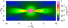 |
Fig. 1 Color map of the initial density of the SN progenitor with M⋆ = 45 M⊙, R⋆ = 80 R⊙ (with mean density |
3 Hydrodynamics and similarity solution of expanding supernova envelope
It is conventional to describe the evolution of a SN remnant in several consecutive phases (e.g., Matzner & McKee 1999). In the early phase the ejecta expands more or less ballistically into the surrounding medium. Ahead of the ejecta a strong shock is driven into the ambient medium while the high pressure behind the forward shock drives a reverse shock into the ejecta (Chevalier 1982; Chevalier & Soker 1989; Truelove & McKee 1999). This “ballistic” or free expansion phase ends when the total amount of material swept up by the forward shock has a mass comparable to that of the ejecta, or equivalently, the mean density of the ejecta drops to that of the surrounding medium.
The basic analytical solution of the SN explosive event follows the idea of homologous (u ∝ r∕t) energy-conserving hydrodynamic expansion, using the Sedov-Taylor blast wave solution (Sedov 1959) and the Sakurai solution of a shock wave in a nonuniform medium (Sakurai 1960) that has different density profiles of an internal gas and surrounding medium (Sedov 1977; Zel’dovich & Raizer 1967). Gravitational force is unimportant except for the very interior layers, and the radiative losses are almost negligible in the early phase of expansion when comparing to a kinetic energy of the gas. We thus may regard the process as adiabatic. The scaling parameters are the energy of explosion ESN, mass Mej of the expanding ejecta, and initial stellar radius R⋆.
The main aim of our study is the modeling of interactions between the spherically expanding SN remnant and the surrounding CSM, which may be spherically symmetric (stellar winds and/or pre-explosion gaseous shells) or asymmetric (circumstellar disks, disk-like density enhancements, and bipolar lobes). Therefore, we neglect a pre-explosion SN interior density distribution, which is completely transformed during the explosion, and on the other hand is of little influence on the structure of the studied interaction. We also do not introduce the complete analytical formalism in this section, and we only briefly review the main relations in the way in which we use these for the comparative semi-analytical solution given in Appendix A.2. For the complete description see the fundamental solutions of, for example, Chevalier (1982) and Nadezhin (1985).
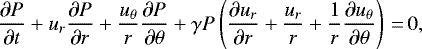
The basic hydrodynamic equations in an axially symmetric slice of spherical coordinates in the plane ϕ = 0, where the angle θ ranges therefore in full angle to include the plane ϕ = π, and where x = R sin θ, z = R cos θ, θ ∈⟨0, 2π⟩ (involving only the terms that are fundamental for nonviscous, non-self-gravitating, and axially symmetric (∂∕∂ϕ = 0) gas expansion), i.e., the continuity equation, radial and polar components of momentum equation, and energy equation, take the form
![\begin{eqnarray}&&\hspace*{-7pt}\frac{\partial\rho}{\partial t}+\frac{1}{r} \frac{\partial}{\partial r}\left(r\rho u_r\right)+ \frac{1}{r}\frac{\partial\left(\rho u_{\theta}\right)}{\partial\theta}\,{=}\, 0,\\[3pt] &&\hspace*{-7pt}\frac{\partial u_r}{\partial t}+u_r\frac{\partial u_r}{\partial r}+ \frac{u_{\theta}}{r}\frac{\partial u_r}{\partial\theta}-\frac{u_{\theta}^2}{r}+ \frac{1}{\rho}\frac{\partial P}{\partial r}-F_0\,{=}\, 0,\\[3pt] &&\hspace*{-7pt}\frac{\partial u_{\theta}}{\partial t}+u_r\frac{\partial u_{\theta}}{\partial r}+ \frac{u_{\theta}}{r}\frac{\partial u_{\theta}}{\partial\theta} +\frac{u_r u_{\theta}}{r}+\frac{1}{\rho r}\frac{\partial P}{\partial\theta}\,{=}\,0,\\[3pt] &&\hspace*{-7pt}\frac{\partial\left(P\rho^{-\gamma}\right)}{\partial t}+ u_r\frac{\left(P\rho^{-\gamma}\right)}{\partial r} +\frac{u_{\theta}}{r}\frac{\left(P\rho^{-\gamma}\right)}{\partial\theta} \,{=}\, 0, \end{eqnarray}](/articles/aa/full_html/2019/05/aa33429-18/aa33429-18-eq11.png)
where ρ is the density, ur is the radial component of the flow velocity, uθ is the polar component of the flow velocity, P is the scalar pressure, F0 is the body force per unit mass (typically gravitation), and γ is the ratio of specific heats. Equation (13) is obtained from the zero total derivative of the adiabatic transformation of a perfect gas Pρ−γ = const. However, we further neglect the gravity term F0 in the momentum Eq. (11), since gravitational force is of very little importance for the studied process.
In the reference frame that is co-moving with the forward shock (for simplicity the planar propagation of the very thin shocked layer) omitting viscosity and assuming constant adiabatic index γ, which is astrophysically relevant (Nadezhin 1985), we can rewrite the adiabatic hydrodynamic Eqs. (10)–(13) on both sides of the shock front into the simple conservative form (Zel’dovich & Raizer 1967),
![\begin{align}&\rho_1 u_1 \,{=}\, \rho_0u_0,\\[1pt] &\rho_1u_1^2+P_1 \,{=}\, \rho_0u_0^2+P_0,\\[1pt] &\frac{\gamma}{\gamma-1}\frac{P_1}{\rho_1}+\frac{u_1^2}{2}\,{=}\,\frac{\gamma}{\gamma-1}\frac{P_0}{\rho_0}+\frac{u_0^2}{2}, \end{align}](/articles/aa/full_html/2019/05/aa33429-18/aa33429-18-eq12.png)
where the upstream and downstream quantities are labeled with subscripts 0 and 1, respectively. The same velocities in the laboratory frame are D − u0 and D − u1, where we denote D the propagation speed of the forward shock. To get the analytical solution, in the early phase after explosion we approximate the process as a free expansion with the internal velocity u of the gas proportional to radius. Assuming the density profile ρin in the envelope as a (time-dependent) power law and the density of the surrounding (initially static) medium ρout as an alternate power law, we obtain
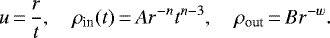 (17)
(17)
Assuming naturally the strong shock condition, Pout ≪ Pin, the proportionality for the inner pressure, Pin ~ ρinu2 (in the shock co-moving frame, or alternatively Pin ~ ρoutD2 in the laboratory frame; see Zel’dovich & Raizer 1967), gives the inner and outer pressure in the form
 (18)
(18)
We describe the formalism of the analytical similarity solution based on Rankine–Hugoniot relations (see the principles given in Chevalier 1982; Nadezhin 1985) in the Appendix A.1, while we describe the principles of semi-analytical model based on analytical solution in Appendix A.2. We also describe in Appendix A.3 the analytical principles of the fundamental limitation of the adiabatic self-similar solution for only a certain time interval. The specific values of this limitation are given within the sections corresponding to the particular models.
4 Numerical method
For the modeling of the interaction with extremely sharp discontinuities characterized by extremely high pressure gradients we have developed and used our own version of single-step (unsplit, ATHENA-like, e.g., Stone et al. 2008) finite volume Eulerian hydrodynamic code based on Roe’s method (Roe 1981; Toro 1999; Kurfürst et al. 2018, see also the description of our geometrical modifications of the algorithm used for different astrophysical situations in Kurfürst & Krtička 2017).
For the time-dependent calculations we write the adiabatic hydrodynamic Eqs. (10)–(13) in two different manners. The primitive form generally is (see, e.g., Stone et al. 2008)
 (19)
(19)
where the primitive variables are W = ρ, u, P, and the fluxes F(W) = ρu, ρu | u + P 1, ρuH, where | denotes the dyadic product of two vectors, H = (E + P)∕ρ is the enthalpy (+ specific kinetic energy), 1 is the unit matrix, and E = ρɛ + ρu2∕2 is total energy (while ɛ is specific internal energy and  ). The primitive (as well as conservative) form of continuity equation is given by Eq. (10), while Eqs. (11) and (12) represent the primitive form of radial and polar components of momentum equation. We transform Eq. (13) into explicit primitive form of energy equation by inserting Eq. (10),
 (20)
(20)
where γ = 4∕3 for the radiation dominated gas. Equations (10)–(12) together with Eq. (20) are used in the primitive numerical scheme (Eq. (19)).
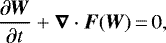
The analogous conservative form is (see, e.g., Norman & Winkler 1986; Hirsch 1989; Stone & Norman 1992; Feldmeier 1995; LeVeque et al. 1998)
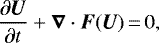 (21)
(21)
where the conservative variables are U = ρ, M, E and F(U) = ρu, M | u + P 1, MH (where M = ρu is the momentum density) for the mass, momentum, and energy equations, respectively. Abbreviating γ′ = γ∕(γ − 1), the explicit adiabatic form of the enthalpy H used in the flux terms is H = γ′P∕ρ + u2∕2. The explicit conservative form of radial (omitting the gravitational force; see Sect. 3) and polar components of momentum equation and of the energy equation, respectively, is
![\begin{align}&\frac{\partial M_r}{\partial t}+\frac{1}{r}\frac{\partial}{\partial r}\left(rM_ru_r\right)+ \frac{1}{r}\frac{\partial(M_{\theta} u_r)}{\partial\theta} -\rho\frac{u_{\theta}^2}{r}+ \frac{\partial P}{\partial r} \,{=}\, 0,\\[4pt]&\frac{\partial M_{\theta}}{\partial t}+\frac{1}{r}\frac{\partial}{\partial r}\left(rM_ru_{\theta}\right)+ \frac{1}{r}\frac{\partial(M_{\theta} u_{\theta})}{\partial\theta} +\rho\frac{u_r u_{\theta}}{r}+\frac{1}{r}\frac{\partial P}{\partial\theta}\,{=}\,0,\\[4pt]&\frac{\partial E}{\partial t}+\frac{1}{r}\frac{\partial}{\partial r}\left(r M_r H\right)+ \frac{1}{r}\frac{\partial}{\partial\theta}\left(M_{\theta} H\right)\,{=}\, 0. \end{align}](/articles/aa/full_html/2019/05/aa33429-18/aa33429-18-eq19.png)
Equation (10) together with Eqs. (22)–(24) are used in the conservative numerical scheme (Eq. (21)).
The polar form of Roe matrices AW = ∂F(W)∕∂W and AU = ∂F(U)∕∂U, resulting from the linearization of Eqs. (19) and (21), is in this case identical and is supplemented by formalism introduced in Stone et al. (2008) and Skinner & Ostriker (2010). We used the (fully capable) second-order piecewise linear reconstruction algorithm, without any necessity to alternate the Roe’s method using the HLLE (Harten, Lax, van Leer, and Einfeldt; cf. Einfeldt et al. 1991; Stone et al. 2008) solver or similar positive-definite solvers in case of unexpected density or pressure drop to negative values in the intermediate states of computation (see Stone et al. 2008, for the details), even in extremely thin zones of very strong shocks.
To derive the initial conditions for hydrodynamic quantities at the explosion time t0 we assumed that the interior shock wave basically rearranges the original density structure of the progenitor. The density gradient between the inner and outer interstellar region is reduced by the rapid expansion of the inner regions (Arnett 1996, see also, e.g., Fig. 1 in Arnould & Prantzos 1986 showing the evolution of the density structure from core collapse to mantle ejection). We therefore neglect the details in a SN interior density structure that can barely affect the main features of examined effects in a complex interaction between SNe and CSM. We thus assume for simplicity that the stellar density is equal to the “averaged” homogeneous initial density  of an exploding star (according to the stellar parameters introduced in Sects. 3, 5, and Appendix A.2) in the range 0.1 − 1 kg m−3 (
 ; cf. Fig. 1).
The injected SN explosion energy is ESN = 1044 J. A SN explosion drives a radiation dominated shock, i.e., the internal energy inside the sphere of shock wave that propagates through the star is dominated by radiation (Nakar & Sari 2010). For that reason we assume the averaged homogeneous initial internal pressure of a photon gas; we consider the whole stellar volume as a “thermal bomb” and neglect the details of the processes connected with the shock wave propagation through the star which, in fact, have a secondary effect on the studied interaction of SN with the aspherical CSM. The averaged homogeneous initial internal pressure of a photon of gas takes the form,  , i.e., in the range between 1010 and 1011 Pa (
 ).
).
We insert the initial state for the CSM in the following explicit form: the density of a spherically symmetric CSM is expressed simply by Eq. (1) while its outflow velocity vsw = 100 km s−1 (see Sect. 2.1 and also Moriya et al. 2014) is used only for initial density estimate and is neglected for the calculation itself. We assume an isothermal initial temperature structure of the CSM (of both the components) within the computational domain, given as Tsw = Tcsd = 0.7Teff (cf. Carciofi & Bjorkman 2008; Kurfürst et al. 2018). This also indicates the initial counterpressure of the CSM as P = ρa2, where the square sound speed a2 is given by Eq. (6). The initial circumstellar equatorial disk density structure (Eqs. (8) and (9)) is in the polar coordinates specified in the following explicit form as
 (25)
(25)
We neglect the velocity field of the circumstellar equatorial disk (see Sect. 2.2), since we regard its effects during the studied process as negligible. The total CSM density profile is given as ρsw (Eq. (1)) + ρcsd (Eq. (25)).
Within our considerations we may set R0 = R⋆, while t0 is certainly less than one day, for example, for SN 1987A the time t0 is estimated to be 53 min after core collapse (Arnett 1996). We set the free boundary conditions at the inner (originally interstellar region) as well as at the outer boundary of the computational domain during the expansion phase. The values for the grid boundary and ghost zones are extrapolated from mesh interior values as a 0th order extrapolation.
We performed all the calculations on a center-symmetric area domain (2D axially symmetric slice of the spherically symmetric 3D domain) with a radius of 20 R⋆, and with a numerical polar grid uniformly scaled in both directions r and θ. The star is located in the center of the computational domain. We also tested the Cartesian uniform grid, interlaced by an equatorial plane of the spherical coordinate system, for comparison with the calculated model; however, we achieved smoother profiles and the optimal computational cost using the polar grid. The number of spatial grid cells was 400 in radial and 300 in azimuthal directions for the models performed up to radius 20 R⋆ and in 2π polar domain. The complete physical time of the simulations corresponds in this case to approximately 165 h. We also performed the calculation on 2D grid containing one polar quadrant (π∕2 polar domain) with 2400 grid cells in radial and 480 grid cells in azimuthal direction with the complete physical time of the simulations corresponding to approximately 180 h. The selected grid aspect ratio has a stabilizing effect because the cells that are stretched along the tangent to the shock have a damping effect on the development of the carbuncle numerical instability (Pandolfi & D’Ambrosio 2001). All the models are described in Sect. 5 (see also Kurfürst et al. 2017, 2018; Kurfürst & Krtička 2017).
Parameters of the three models A, B, and C.
5 Numerical models
We selected a BSG star with M⋆ = 45 M⊙, R⋆ = 80 R⊙, Teff = 25 000 K as the progenitor for all studied models; all of the parameters of this star are described in Sect. 4 (see also Fig. 1). The assumed properties of CSM of studied models (denoted as Model A, B, and C), i.e., the adopted mass-loss rates Ṁ and the approximate base densities ρ0,sw and ρ0,csd derived from the mass conservation equation (see Sects. 2.1 and 2.2), are given in Table 1. In all models we assume vsw = 100 km s−1 (Moriya et al. 2014, see also Sect. 4), which is an order of magnitude latitudinally averaged estimate considering the effects of possible high rotation (Maeder & Meynet 2000; Kraus et al. 2008, 2010) and high radiation pressure.
5.1 Model A: high density of the surrounding media
We first study the SN–CSM interaction for the case of high density of surrounding media. The CSM consists in the spherically symmetric component and the aspherical circumstellar disk described in Sect. 2. The parameters of the CSM and progenitor star are given in Table 1 and in the first paragraph of Sect. 5.
Integrating the density profiles, we estimate the total mass of the CSM components: for spherically symmetric component of CSM we obtain the total mass 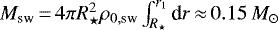 within the radius r1 = 20 R⋆ (within the radius of the computational domain), while we obtain the total mass for circumstellar disk component within the same domain as
  (cf. Krtička et al. 2011; Kurfürst et al. 2014, 2018).
We show in Figs. 2 and 3 the 2D snapshots of density, velocity, and temperature, in equatorial (x)–polar (z) plane, at selected times t = 16 h (only density) and t = 66 h. We also add illustratively separated 1D slices of the graphs of selected quantities in equatorial plane and in polar direction in Fig. 4 at the time t ≈ 66 h, supplemented by a graph of specific radiation entropy s = 16σT3∕(3cρ), where σ is the Stefan-Boltzmann constant and c is the speed of light (Zel’dovich & Raizer 1967). The figures show the regions of decelerated expansion velocity toward the equatorial disk while the expansion is unlimited (relatively, according to the density of the spherically symmetric CSM component) in the polar direction. All the characteristics show enhanced peaks in the SN-disk contact region and indicate shoulders and strips of overdensity and enhanced temperature that propagate around the equatorial disk.
We show in the upper panel of Fig. 5 the density slopes n and w (see Eqs. (17) and (A.1)) and in the lower panel of Fig. 5 the temperature slopes p (cf. Eq. (5)), calculated in the numerical model at the same time t ≈ 66 h since shock emergence. However, the outer shock, which roughly separates the outer region (denoted in Sect. 3 by subscript“out”) from all the other regions between the two shock waves, moves to the radius approximately 11 R⋆ in the equatorial plane and 16.5 R⋆ in the polardirection. The inner envelope density slope ranges in the polar direction between n = 0 and n ≈ 9, while in the equatorial plane the density slope is highly discontinuous and becomes much steeper. However, we cannot simply apply the analytical similarity relations in the equatorial plane with respect to the constraint w <3 given by Eq. (A.21). The temperature slope in the smooth region of the inner envelope (excluding the areas of sharp discontinuities) ranges between p = 0 and p ≈ 2.7 in the equatorial and in the polar direction. In order to avoid inadequate computational difficulties, we calculate the temperature in all the domain as radiative (T ~ P0.25; the same applies for the other models). We may regard the displayed distances reached by the forward shock wave in the equatorial and in the polar direction as a certain scale of the level of asphericity (except the slopes of the selected quantities) of the SN explosion; the same also applies for another models (see Figs. 11 and 18).
In Figs. 6 and 7 we demonstrate the semi-analytically found (see Sect. A.2) similarity solution of density, velocity, pressure, and temperature for two inner density slopes n = 7 and n = 9 that correspond to the average and maximum numerically calculated inner density slopes in the polar direction where the similarity solution holds and where the parameter w < 3 (see Eq. (A.1) and its consequences). In the disk-residing equatorial plane the analytical similarity solution is however violated because of the disk equatorial plane density profile ρeq (R) ~ R−3.5 (w > 3).
Comparing slices of 2D numerical calculations in Fig. 4 with the 1D semi-analytical solution (cf. Sect. A.2) in polar direction in Figs. 6 and 7, we find that the solutions well agree in global parameters. That is, density ρ decreases from the value ρ ≈ 5 × 10⁻⁶ kg m−3 at the radius r = 11.5 R⋆ to ρ ≈ 3 × 10⁻⁷ kg m−3 behind the outer shock, while it drops to almost 10−8 kg m−3 outside the outer shock; the radial (expansion) velocity u grows in the same domain from u ≈ 3000 km s−1 to approximately 3500 km s−1 behind the shock wave zone. We hereafter denote the radial velocity of expansion u for simplicity; its value in fact does not much differ from the total magnitude of velocity since the nonradial velocity components are more than an order of magnitude smaller. The pressure approaches P ≈ 106 Pa, while the corresponding temperature T is slightly higher than 105 K (compare Figs. 6 and 7 with Fig. 4). The semi-analytical solution is directly compared with 1D slices of our 2D numerical solution for the same time of calculation. We also add the 1D synchronous profile calculated using the SNEC-1.01 code (Morozova et al. 2015), which takes into account more realistic shape of the density enhancement zone between reverse shock and contact discontinuity (between 13.5 and 13.8 r∕R⋆) that is formed during propagation of the shock wave through the stellar body (Sedov 1959; Sakurai 1960). Since our current models use the whole stellar body as an initial thermal bomb, the shock wave directly propagates (like a Riemann-Sod shock wave) to the region of dropped density. However, this detail in the shock wave structure has only a minor impact on the global solution within the study. For the SNEC calculation we input the same initial profile of the progenitor star and the CSM as for all the other calculations with radiation included, the initial thermal bomb zone (Morozova et al. 2015) is however limited only to a relatively small region near the stellar center.
We also constructed similar comparative diagrams for other values of parameter n lower than n = 7. However, in this case the radial distance between the inner and outer shock waves becomes too large and the values of analytically calculated quantities differ significantly from SNEC and from our 2D numerical result. In any case, we found that the analytical versus numerical solutions are closest (relatively) at this stage for the internal density slope parameter n ≈ 7 to n ≈ 9.
We also checked the constraints on the applicability of the adiabatic self-similar solution within the semi-analytical calculation (see Appendix A.3). For the model with high density (Sect. 5.1) and the density slope n = 7 we found the upper limit tmax ≈ 20 yr, while the lower limit tmin is on the order of several minutes at the start of the calculation. The lower limit continuously grows during the time evolution, however, the values of tmin remain several orders of magnitude lower than the actual time of simulation.
Figure 3 indicates that the zone of shear between the slower expansion into the region of circumstellar equatorial disk, where the vertical motion occurs owing to the violation of disk hydrostatic equilibrium caused by the interaction of the two masses. Figure 3 also shows that the spherically symmetric fast SN expansion may provoke the development of Kelvin-Helmholtz instabilities. This is further demonstrated in Fig. 8, where we show the snapshot of 2D density and expansion velocity field in later time t ≈ 165 h (up to the radius 50 R⋆) and in higher numerical resolution. We thus get a comparison with the model in Fig. 3, where we can distinguish the details of evolution of the selected quantities in yet more evolved and more structured stage. The shoulders of overdensity and significantly decelerated expansion velocity at the zone of shear between the disk and spherically symmetric CSM are illustrated in a more detailed picture. There is also a clear indication of developing Kelvin-Helmholtz and Rayleigh-Taylor instabilities along the zone of shear interaction and SN-disk contact region.
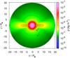 |
Fig. 2 Model A: color map of the density structure of the interaction of SN (with progenitor and CSM parameters introduced in Sect. 3, Table 1, and in Fig. 1) with asymmetric CSM that forms a dense equatorial disk, at time t ≈ 16 h since shock emergence. Contours denote the densities ρ = 10−7, 10−6, 10−5, and 10−4 kg m−3. |
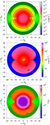 |
Fig. 3 Model A: interaction of SN with asymmetric CSM at time t ≈ 66 h since shock emergence. Upper panel: color map of the density structure. Contours denote the densities ρ = 10−6, 10−5, and 10−4 kg m−3. Middle panel: color map of the velocity structure. Contours denote the radial (expansion) velocities u = 1000, 2000, and 3000 km s−1. Lower panel: color map of the temperature structure. Contours denote the temperatures T = 105, 5 × 10⁵, and 106 K. Characteristic 1D sections of the model in the equatorial and polar plane are shown in Fig. 4. |
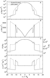 |
Fig. 4 Model A: one-dimensional slices of variations of hydrodynamical variables in the equatorial plane (x-coordinate, solid line) and in the polar direction (z-coordinate, dashed line), at the same time as in Fig. 3. Panel A: density ρ. Panel B: expansion velocity u. Panel C: pressure P and temperature T. Panel D: specific entropy s. |
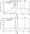 |
Fig. 5 Model A: upper panel: slope parameters n and w of the density (see Eq. (17)) in the equatorial (solid line) and polar (dashed line) direction corresponding to the panel A in Fig. 4, at the same time. The position of the outer shock wave is at r ≈ 11 R⋆ in the equatorial direction, while it is at r ≈ 16.5 R⋆ in the polar direction. There are preserved the initial density slope parameters of CSM, wsw = 2 in the polar direction and wcsd = 3.5 in the equatorial direction, above these radii. The inner envelope density slope parameter increases from n = 0 to n ≈ 9 in the polar direction. The numbers nmax and nmin above and below the graph denote the maximal and minimal slopes within the peaks of the density gradient discontinuities. Lower panel: slope parameters p of the temperature (cf. Eq. (5)) in the equatorial (solid line) and polar (dashed line) direction corresponding to the temperature graph (panel C) in Fig. 4 at the same time. The inner envelope (smooth) temperature slope parameter increases to p ≈ 2.7 at r ≈ 7.8 R⋆ in the equatorial direction while it increases to approximately the same value at r ≈ 11 R⋆ in the polar direction. The slope parameter p outside the outer shock is p = 0.875 in the equatorial and p = 0.5 in the polar direction. The numbers pmax above the graph denote the maximal temperature slopes within the peaks of the T gradient discontinuities. |
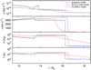 |
Fig. 6 Model A: results of semi-analytical solution of the density ρ, velocity u, pressure P, and temperature T (black line), with the slope parameters n = 7 and wsw = 2, in the polar direction. The method of calculation is described in Sect. A.2. The time is the same as in Figs. 3–5. The velocity at the outer shock wave region (at approx. 16 R⋆) correspondsto the polar expansion velocity in the panel B of Fig. 4 while the other quantities and semi-analytical model input variables are described in Appendix A.2. The blue line depicts the corresponding calculation from our 2D model. The corresponding 1D profile calculated using the SNEC-1.01 code is depicted with a red line (see the description in Sect. 5.1). |
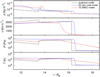 |
Fig. 7 Model A: as in Fig. 6, with the slope parameters n = 9 and wsw = 2, in the polar direction (the same method of calculation as in Fig. 6). The semi-analytical profiles are compared to the same polar expansion velocity as in Figs. 4 and 6. |
5.2 Model B: intermediate density
We further studied interaction of an SN blast wave with the CSM for the case of intermediate density (Model B). The progenitor and CSM parameters are introduced in the first paragraph of Sect. 5 and in Table 1. Integrating the CSM density profiles, we obtain the following total mass of the CSM components: the total mass Msw ≈ 0.015 M⊙ within the radius of the computational domain r1 = 20 R⋆ and Mcsd ≈ 0.65 M⊙ (cf. Krtička et al. 2011; Kurfürst et al. 2014, 2018) within the same domain.
We show (analogous to Sect. 5.1) in Fig. 9 the 2D snapshots of density profiles in equatorial (x)–polar (z) plane at selected times t = 33 h and t = 66 h, respectively.The lower panel in Fig. 9 shows significant layers of overdensity that are formed near the zone where the expanding matter is forced to move along the interface between the spherically symmetric component of CSM and the denser circumstellar equatorial disk region of CSM. The development of Kelvin-Helmholtz instabilities is also remarkably indicated near the shear zones. We also add in Fig. 10 the separated 1D slices of graphs of density, velocity, pressure, temperature, and specific radiation entropy in equatorial and polar plane at the time t = 33 h. The model shows higher difference in expansion velocity between the equatorial and polar direction than in the previous model because of the lower density (lower mass injection) of spherically symmetric CSM. The front of the polar SN expansion reaches the velocity approximately 4000 km s−1 while it approaches 2000 km s−1 in the equatorial direction. Because the expansion shock front in the polar direction is too close to the limit of computational area in the time for which we plotted the previous models (t ≈ 66 h), we provide for this model the profiles of most of the characteristics in earlier time (t ≈ 33 h) while, on the other hand, the graphs of the previous model with high density would be in this time poorly illustrative.
We also show (analogously to Sect. 5.1) in the upper panel of Fig. 11 the density slopes n and w, while in the lower panel we show the temperature slopes p, calculated at the same time t ≈ 33 h since shock emergence. The outer shock moves at the radius of approximately 5.5 R⋆ in the equatorial and 11 R⋆ in the polar direction. The inner envelope density slope ranges in the polar direction between n = 0 and n ≈ 16, the temperature slope in the smooth region of the inner envelope ranges between p = 0 and p ≈ 1.9 in the equatorial direction and between p = 0 and p ≈ 3.6 in the polar direction.
The calculation of the constraints of applicability of the adiabatic self-similar solution (see Appendix A.3) gives for the model with intermediate density the upper limit tmax ≈ 21 yr for the density slope n = 7, while for n = 12 it increases to tmax ≈ 35 yr. For the lower limit tmin applies the same as in previous model with high density in Sect. 5.1.
Analogous to the previous model, we show in Fig. 12 the snapshots of 2D density, radial expansion velocity, and temperature in time t ≈ 180 h since shock emergence, up to the radius 50 R⋆, in high numerical resolution, performed on 2D grid with 2400 grid cells in radial and 480 grid cells in azimuthal direction. Comparing this with Fig. 9, we distinguish the details of evolution of the selected quantities, including the even more significant shoulders of overdensity and over-heated gas near disk – spherically symmetric CSM shear zone. Although the forward shock front is in the snapshot already out of the computational domain, it particularly well illustrates the development of Kelvin-Helmholtz and Rayleigh-Taylor instabilities which is clearly indicated.
We also add in this intermediate density model the 1D equatorial, polar slices of density and expansion velocity (Fig. 13), and the temperature and specific entropy (Fig. 14), which correspond to the instant time shown in Fig. 12. A qualitative comparison with the profiles in Fig. 10 (in less advanced time) shows the decrease of density, however in a (roughly) self-similar mode. This is accompanied by an increase of the equatorial velocity peak. The peak of the polar velocity is currently already outside the computational domain, nevertheless the results of the calculation before it reaches the outer boundary show that the polar velocity increases very little (cf. the increase of polar velocity in the model with high density (Sect. 5.1) by comparing the values of the polar velocity maximum in Figs. 3 and 4 with Fig. 8).
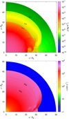 |
Fig. 8 Model A: detailed color maps of the density (upper panel) and the radial velocity (lower panel) structure, up to the distance 50 R⋆ at time t ≈ 165 h since shock emergence. Contours denote the densities ρ = 10−7, 10−6, and 10−5 kg m−3 and the velocities 2500 and 3000 km s−1. The resolution of the simulation is 2400∕480 grid cells in the radial/azimuthal direction within the quadrant. |
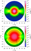 |
Fig. 9 Model B: upper panel: color map of the density structure at time t ≈ 33 h since shock emergence. Contours denote the densities ρ = 10−8, 10−7, 10−6, 10−5, and 10−4 kg m−3. Characteristic 1D sections of the model in the equatorial and polar plane are shown in Fig. 10. Lower panel: color map of the density structure at time t ≈ 66 h since shock emergence. Contours denote the densities ρ = 10−6, 10−5, and 10−4 kg m−3. |
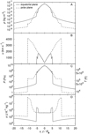 |
Fig. 10 Model B: 1D slices of hydrodynamical variables in the equatorial plane (x-coordinate, solid line) and polar plane (z-coordinate, dashed line) at time t ≈ 33 h since shock emergence (as in Fig. 9). Panel A: density ρ. Panel B: expansion velocity u. Panel C: pressure P and temperature T. Panel D: specific entropy s. |
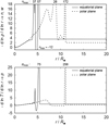 |
Fig. 11 Model B: upper panel: slope parameters n and w of the density (analogous to Fig. 5) in the equatorial (solid line) and polar (dashed line) direction, corresponding to panel A in Fig. 10 at the same time t ≈ 33 h. The positionof the outer shock wave is at r ≈ 5.5 R⋆ in the equatorial direction, while it is at r ≈ 11 R⋆ in the polar direction. The inner envelope density slope parameter increases from n = 0 to n ≈ 16 in the polar direction. Lower panel: slope parameters p of thetemperature in the equatorial (solid line) and polar (dashed line) direction corresponding to the temperature graph (panel C) in Fig. 10 at the same time. The inner envelope (smooth) temperature slope parameter increases to p ≈ 1.9 at r ≈ 4.1, R⋆ in the equatorial direction while it increases to p ≈ 3.6 at r ≈ 6.6 R⋆ in the polar direction. |
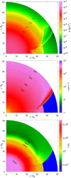 |
Fig. 12 Model B: detailed color maps of the density (upper panel), radial velocity (middle panel), and temperature (lower panel) structure up to the distance 50 R⋆ at time t ≈ 180 h since shock emergence, with the same numerical resolution as in Fig. 8. Contours denote the densities ρ = 10−7, 10−6, 10−5, and 10−4 kg m−3, the velocities 2500, 3000, 3500, and 4000 km s−1, and the temperatures 7 × 10⁴, 8 × 10⁴, 105, and 5 × 10⁵ K. |
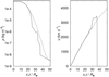 |
Fig. 13 Model B: 1D slices of density (left panel) and velocity (right panel)in the equatorial plane (x-coordinate, solid line) and in polar direction (z-coordinate, dashed line) at time t ≈ 180 h since shock emergence (corresponding to Fig. 12). The maximum of the polar velocity, which is already outside the computational domain, is approximately 4400 km s−1. |
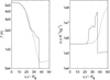 |
Fig. 14 Model B: 1D slices of temperature (left panel) and specific entropy (right panel) in the equatorial (x-coordinate, solid line) and in polar direction (z-coordinate, dashed line)at the same time as in Fig. 13. |
5.3 Model C: low density
The asymetry of SN–CSM interaction zone is significant even in the case of low density CSM (Model C). The progenitor and CSM parameters are introduced in the first paragraph of Sect. 5 and in Table 1. The total masses of the spherical wind and circumstellar equatorial disk components within the radius of the computational domain r1 = 20 R⋆ are Msw ≈ 1.5 × 10⁻⁴ M⊙ and Mcsd ≈ 6.5 × 10⁻³ M⊙.
We show (analogous to Sects. 5.1 and 5.2) in Figs. 15 and 16 the 2D snapshots of density, velocity, and temperature, in equatorial (x)–polar (z) plane, at selected times t = 33 h and t = 66 h (only density). We again also add in Fig. 17 the separated 1D slices of graphs of density, velocity, pressure, temperature, and specific radiation entropy in equatorial plane and in polar direction at the time t = 33 h. The figures in this case show the regions of significantly decelerated SN expansion velocity toward the equatorial disk in greater distance from the star than in the previous cases; in the corresponding time t ≈ 66 h it is approximately 13 R⋆ (see Fig. 16), while it is approximately 11 R⋆ in the previous models (cf. Figs. 4 and 10). This is because the higher absolute value of expansion velocity even in this direction of maximum deceleration compared to previous models (cf. also Figs. 3, 9, and 17). The front of the polar SN expansion propagates with much higher velocity, i.e., > 7000 km s−1 while it is ≈ 4000 km s−1 in the model with intermediatedensity and ≈3000 km s−1 in the model with high density in the same direction at the same time; the front should be within the same time t ≈ 66 h obviously in much larger distance than in the previous models. This is why, outside the computational area, we plot in this model the profiles of most of the characteristics in time t ≈ 33 h.
We show (analogous to Sects. 5.1 and 5.2) in the upper panel of Fig. 18 the density slopes n and w and in the lower panel the temperature slopes p, calculated at the same time t ≈ 33 h since shock emergence. The outer shock moves at the radius of approximately 9 R⋆ in the equatorial plane and 18 R⋆ in the polar direction. The inner envelope density slope ranges in the polar direction between n = 0 and n ≈ 17; the temperature slope in the smooth region of the inner envelope ranges between p = 0 and p ≈ 3.6 in the equatorial and also in the polar direction.
The calculation of the applicability limits of the adiabatic self-similar solution (see Appendix A.3) gives for the model with low density the upper limit tmax ≈ 190 yr for the density slope n = 7, while for n = 12 it gives tmax ≈ 3 × 10⁴ yr. The lower limit tmin is still practically unimportant (cf. the model with high density in Sect. 5.1).
As in both the previous models, we show in Fig. 19 the snapshots of 2D density and expansion velocity in a more evolved stage (in time t ≈ 105 h since shock emergence), up to the radius 50 R⋆, performed on 2D grid with 2400 grid cells in radial and 480 grid cells in azimuthal direction. Comparing this with Fig. 15, we distinguish again the details of evolution of the selected quantities within the model.
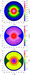 |
Fig. 15 Model C: color maps of the hydrodynamical variables at time t ≈ 33 h since shock emergence. Upper panel: color map of the density structure. Contours denote the densities ρ =10−8, 10−7, 10−6, 10−5, and 10−4 kg m−3. Middle panel: color map of the velocity structure. Contours denote the velocities u = 5000 and 7000 km s−1. Lower panel: color map of the temperature structure. Contours denote the temperatures T = 105 and 106 K. Characteristic 1D sections of the model in the equatorial plane and in the polar direction are shown in Fig. 17. |
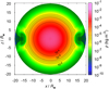 |
Fig. 16 Model C: color map of the density structure of the interaction at time t ≈ 66 h since shock emergence. Contours denote the densities ρ = 10−6, 10−5, and 10−4 kg m−3. |
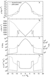 |
Fig. 17 Model C: 1D slices of hydrodynamical variables in the equatorial (x-coordinate, solid line) and in polar direction (z-coordinate, dashed line) at time t ≈ 33 h since shock emergence (as in Fig. 15). Panel A: density ρ. Panel B: expansion velocity u. Panel C: pressure P and temperature T. Panel D: specific entropy s. |
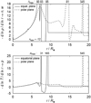 |
Fig. 18 Model C: upper panel: slope parameters n and w of the density (analogous to Figs. 5 and 11) in the equatorial (solid line) and polar (dashed line) direction, corresponding to panel A in Fig. 17 at the same time t ≈ 33 h. The positionof the outer shock wave is at r ≈ 9 R⋆ in the equatorial direction while it is at r ≈ 18 R⋆ in the polar direction. The inner envelope density slope parameter increases from n = 0 to n ≈ 17 in the polar direction. Lower panel: slope parameters p of thetemperature in the equatorial (solid line) and polar (dashed line) direction corresponding to the temperature graph (panel C) in Fig. 17 at the same time. The inner envelope (smooth) temperature slope parameter increases to p ≈ 3.6 at r ≈ 6.3–6.5 R⋆ in the equatorial and also in the polar direction. |
6 Conclusions and future work
We studied the hydrodynamic behavior of interaction between the expanding envelope of SNe and aspherical CSM containing an spherically symmetric stelar wind component and an aspherial circumstellar equatorial disk (or disk-like) component that is axially symmetric and resides in the equatorial plane of the star. In the present model we used simplified initial conditions, assuming homogeneous initial distribution of the stellar density and pressure without gravity, which has only a minor impact on the studied process of external interaction.
We discussed three particular 2D models, supplemented by 1D illustrative slices of basic hydrodynamic quantities and of gradients (slopes) of density and temperature, for three different values of stellar pre-explosion mass-loss rate that led to formation of CSM. All the models significantly demonstrate the higher rate of deceleration of SN expansion in case of higher density of CSM and the aspherical evolution of the density, velocity, and temperature structure of the SNe ejecta, where the mass preferably expands to the area outside the dense equatorial disk (cf. McKee & Cowie 1975; McKee et al. 1978; Cowie et al. 1981). We conclude that in case the disk initial base density values ρ0,csd are of an order of magnitude (or more) higher than the base densities ρ0,sw of spherically symmetric CSM, such circumstellar equatorial disks effectively slow down the equatorial SN expansion (compared to the SN expansion into regions outside the disk) with significant peaks of density, pressure, and temperature in the contact region of SN-disk interaction. This is according to the presented models and other models with even lower initial CSM densities down to Ṁcsd ≈ 10−9 M⊙ yr−1 with ρ0,csd of an order of 10−9 kg m−3, where the effects of asphericity vanish, and down to Ṁsw ≈ 10−7 M⊙ yr−1 with ρ0,sw of an order of 10−12–10−11 kg m−3 below whichthe effects of CSM become negligible. The comparison of power-law gradients of density and temperature (basically described in Figs. 5, 11, and 18), at least for the smooth parts of the expanding area (excluding the regions of steep shocks and discontinuities), indicates their higher values for lower pre-explosion mass-loss rates. The slopes also decrease with time, however, this can be expected from the similarity nature of expansion. We also checked the time limits of similarity solution applicability, where all the models match the time frame with considerable reserve.
The models also indicate the development of Kelvin-Helmholtz instabilities in the zone of shear where the expanding matter flow is distorted along the interface between the spherically symmetric component and circumstellar equatorial disk component of CSM, forming the nearby layers of overdensity.
In our models, we did not consider the effects of radiative cooling, the influence of magnetic fields, or the energy input from the compact remnant of the explosion. These effects are typically mitigated and overlapped by the enormous SNe energy and their impact on the dynamics of the problem is very small (Truelove & McKee 1999), or are connected only with a specific situation or a type of the remnant (like magnetars; see, e.g., Metzger et al. 2017). The reverse shock formed in uniform ejecta is assumed to be radiative for a certain time (Chevalier 1977), but its velocity becomes eventually so high and the ejecta are so tenuous that the cooling timescale for the gas behind the shock exceeds the dynamical time of the SN expansion (Truelove & McKee 1999). It is therefore relevant to use the nonradiative approximation. In this point, Truelove & McKee (1999) showed that the fraction of ejecta mass that cools is only a few percent in the case of n < 5 ejecta, in case of typical values of parameters. Moreover, Chevalier & Fransson (1994) studied the early radiative period for n > 5 ejecta and found it had very little effect upon the dynamics of the SN expansion.
Because of the inclusion of radiative cooling, and therefore a violation of the energy conservation, the shocked shell becomes thinner and denser than in the case of the used self-similar analytical description (Chevalier 1982). Such a shell is however expected to be unstable because of developing (the Rayleigh-Taylor) instabilities (e.g., Chevalier & Blondin 1995), whose effect reduces the rate of conversion of the kinetic energy to radiation (Blinnikov et al. 1998; Moriya et al. 2013a). These instabilities are usually included in 1D models via an approximative “smearing term” (similar in principle to the numerical viscosity). We currently omit such details owing to the complexity of the SN–CSM interaction morphology, but they may be included in the future calculations (cf. the study of Steinberg & Metzger 2018).
Although the detailed description of observational signatures connected with the conclusions of the models is not the subject of this paper, we briefly comment on that issue. From an analytic solution suggested, for example, by McDowell et al. (2018; see also Moriya et al. 2013b or Chatzopoulos et al. 2013), it follows that in cases in which the mass of the disk Mcsd is comparable with the mass of the ejecta Mej, the ratio of the luminosity of the light curve peak is approximately indirectly proportional to the SN diffusion timescale τsn; the time when the opacity drops so that the radiation can freely escape. In cases in which the mass of the disk is much smaller (two orders of magnitude or more) than the ejecta mass, then the peak luminosity ratio of the light curve is significantly reduced; the peak luminosities for the same ratio of the SN diffusion times are much closer. Comparing the first two models A and B (where Mcsd is comparable with Mej ≡ M⋆) with model C, we obtain a ratio of the diffusion timescales of about 3∕2. We may thus expect the light curve peak ratio to be approximately 1.2–1.5 in favor of model C. We may also assume that in case of yet lower disk masses the difference in luminosities would be even less distinct. However, the situation may be complicated according to the line of sight of an observer. We expect that in the case of pole-on observational direction the difference in light curve luminosities would be much smaller (if any) while in case of equator-on (disk-on) observational direction the effects of the disk may correspond to the above estimate. We also expect that because of the asymetry of the outflow the resulting line profiles should depend on the direction of observation showing higher outflow velocities in the polar direction than in the equator-on direction.
As an immediate future step we plan to modify the initial stellar profiles of the density and temperature into a more realistic form, including the internal structure of the progenitor pre-calculated from stellar evolution code. We also compare the current 2D models calculated without gravity with the models with the stellar gravity included. However, in this point we checked the influence of the gravitational force on the expansion profiles using the 1D SNEC calculations, and there is a remarkable impact only in the central region of the original progenitor, which expands self-similarly together with the expansion of the whole envelope. For future 2D models we will implement the equilibrium-diffusion radiation transport solver into the code, taking into account recombination effects in the envelope and the effects of radioactive heating. This will enable us to perform the calculations in radiation-hydrodynamic mode with radiation-matter coupling.
We expect that subsequent study of the SN light curves powered by SN thermal energy excess will lead to a better understanding of the mass and density distribution of the CSM. It may also provide more precise estimates of the disk mass-loss rates and a deeper knowledge of the geometry and mechanism of the mass loss of massive stars.
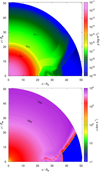 |
Fig. 19 Model C: detailed color maps of the density (upper panel) and radial velocity (lower panel) up to the distance 50 R⋆ at time t ≈ 105 h since shock emergence, with the same resolution as in Fig. 8. Contours denote the densities ρ = 10−7, 10−6, 10−5, and 10−4 kg m−3 and the velocities 5000 and 7000 km s−1. |
Acknowledgements
We thank Dr. Ondřej Pejcha for helpful comments on details of the studied (or similar) process. We are also gratefulto Milan Prvák for technical support in preparation of the draft of this paper. The access to computing and storage facilities owned by parties and projects contributing to the National Grid Infrastructure MetaCentrum, provided under the program “Projects of Large Infrastructure for Research, Development, and Innovations” (LM2010005) is appreciated. This work was supported by the grant GA ČR 18-05665S and by the grant Primus/SCI/17.
Appendix A Analytical solution of SN expansion
A.1 Basics ofadiabatic similarity solution
Contact discontinuity separates the SN remnant and CSM and propagates among the forward and reverse shock wave. An analytical approach requires a similarity solution (see, e.g., the formalism in Chevalier 1982 or Nadezhin 1985) with the coefficient of proportionality λ(r, t) defined as Kλ(r, t) = rt−α (where the parameter α is different from αvis in Sect. 2and K is the scaling constant). Denoting λI = 1 the value of λ at the inner (reverse) shock wave, λC at the contact discontinuity, and λII at the outer forward shock wave (where obviously λin(r < rI) < λI < λC < λII < λout(r > rII)), coupling of the densities in Eq. (17) gives
 (A.1)
(A.1)
Substituting the equations for λ and α into Eq. (17), we introduce the similarity variables U(λ), V (λ), W(λ), and C(λ), which correspond to velocity, density, pressure, and sound speed. The equations for u, ρ, and P are
![\begin{align}&u(r\le r_{\text{II}})\,{=}\,Kt^{\alpha-1}\lambda U(\lambda),\nonumber\\[6pt] &u(r>r_{\text{II}})\,{=}\,0,\\[6pt] &\rho(r\le r_{\text{C}})\,{=}\,AK^{-n}t^{-\alpha w}V(\lambda),\nonumber\\[6pt] &\rho(r>r_{\text{C}})\,{=}\, BK^{-w}t^{-\alpha w}V(\lambda),\\[6pt] &P(r\le r_{\text{C}})\,{=}\,AK^{2-n}t^{\alpha(2-w)-2}\lambda^2W(\lambda),\nonumber\\[6pt] &P(r>r_{\text{C}})\,{=}\, BK^{2-w}t^{\alpha(2-w)-2}\lambda^2W(\lambda).\end{align}](/articles/aa/full_html/2019/05/aa33429-18/aa33429-18-eq28.png)
The similarity variable C(λ) is defined as C2 = γW(λ)∕V (λ). Following the relation for the coefficient λ, we may express the velocity uC of the contact discontinuity,
 (A.5)
(A.5)
Substituting Eqs. (A.2)–(A.4) for the domain r ≤ rII into Eqs. (10)–(13), assuming spherical symmetry, and partially differentiating with respect to t and λ, we obtain the following similarity relations (cf. Nadezhin 1985) for the continuity, momentum, and energy equations, respectively,
 (A.6)
(A.6)
 (A.7)
(A.7)
![\begin{align*}\lambda\left(U-\alpha\right)\left[(1-\gamma)\frac{V^{\prime}}{V}+ 2\frac{C^{\prime}}{C}\right]+2(U-1)+(\gamma-1)\alpha w\,{=}\,0. \end{align*}](/articles/aa/full_html/2019/05/aa33429-18/aa33429-18-eq32.png) (A.8)
(A.8)
The explicit form of Eqs. (A.6)–(A.8) for each particular similarity variable derivative is
![\begin{align*}\lambda U^{\prime}\,{=}\,-\frac{\mathcal{S}C^2+\left(U-\alpha\right)[3C^2-U(U-1)]}{C^2-\left(U-\alpha\right)^2}, \end{align*}](/articles/aa/full_html/2019/05/aa33429-18/aa33429-18-eq33.png) (A.9)
(A.9)
![\begin{align*}\lambda\frac{V^{\prime}}{V}\,{=}\,\frac{\eta\mathcal{S}C^2+\left(U-\alpha\right) [\left(U-\alpha\right)(3U-\alpha w)-U(U-1)]} {\left(U-\alpha\right)[C^2-\left(U-\alpha\right)^2]}, \end{align*}](/articles/aa/full_html/2019/05/aa33429-18/aa33429-18-eq34.png) (A.10)
(A.10)
![\begin{eqnarray*} \hspace*{-6pt}&&\lambda\frac{C^{\prime}}{C}=-\frac{\eta\mathcal{S}C^2}{2\left(U-\alpha\right) [C^2-\left(U-\alpha\right)^2]}\nonumber\\ \hspace*{-6pt}&&\quad+\,\frac{2C^2+(\gamma-1)U(U-1)+\left(U-\alpha\right)[2-(3\gamma-1)U]} {2[C^2-\left(U-\alpha\right)^2]},\end{eqnarray*}](/articles/aa/full_html/2019/05/aa33429-18/aa33429-18-eq35.png) (A.11)
(A.11)
where we substitute the constant expressions η and  ,
,
 (A.12)
 (A.13)
Multiplying Eq. (A.6) by an auxiliary constant β and subtracting it from Eq. (A.8), the integration gives the implicit adiabaticity integral (see, e.g., Sedov 1959; Nadezhin 1985)
 (A.14)
where the constant β is
 (A.15)
The Rankine–Hugoniot relations (e.g., Zel’dovich & Raizer 1967) give the λ-independent similarity variables for the inner strong shock,
 (A.16)
The similarity variables for the outer strong shock are
 (A.17)
where only the variable VII has to be evaluated numerically using the principles given in Appendix A.2.
We also express the similarity variables in the zones inside the inner shock wave (λin < 1) and outside the outer shock wave (λout > λII). Combining Eq. (17) with Eqs. (A.2)–(A.4) and assuming uout, Pin, Pout = 0, we obtain
![\begin{align}&U_{\text{in}}\,{=}\,1,\quad V_{\text{in}}\,{=}\,\lambda_{\text{in}}^{-n},\quad C_{\text{in}}\,{=}\,0,\\[4pt] &U_{\text{out}}\,{=}\,0,\quad V_{\text{out}}\,{=}\,\frac{\gamma-1}{\gamma+1}\left(\frac{\lambda_{\text{II}}} {\lambda_{\text{out}}}\right)^{w}V_{\text{II}},\quad C_{\text{out}}\,{=}\,0.\end{align}](/articles/aa/full_html/2019/05/aa33429-18/aa33429-18-eq43.png)
From Eq. (A.9) it follows that in very proximity of the contact discontinuity (where U − α → 0)  . Integrating the left-hand side of this relation from U(λC) to a nearby U and the right-hand side from λC to a nearby λ, as well as integrating analogously Eqs. (A.10) and (A.11), gives the similarity relations close to rC in the form
 (A.20)
where ξ and ζ are arbitrary constants that differ in general on both sides of rC. However, since u and P are continuous (Zel’dovich & Raizer 1967) through rC (implying a constant product V C2 in Eq. (A.20)), we may write  , where the subscript “i” denotes the zone between the inner shock wave and the contact discontinuity while the subscript “o” denotes the zone between the contact discontinuity and the outer shock wave. To determine the constants ξ and ζ, Eq. (A.20) have to be calculated numerically within the semi-analytical solution (see Appendix A.2).
We obtain the relations for total mass MI,II and total energy EI,II confined between the two shocks (Nadezhin 1985) by integration of Eq. (17), with use of the formalism in this section,
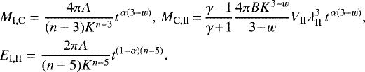 (A.21)
This leads to the important constraint w < 3 and n > 5 for the similarity solution, while Eq. (A.1) implies the condition α < 1.
To evaluate the constants A, B, and K, we identify the mass Mej of the SN envelope as MI,C (which tends to be relevant in an advanced time) and the energy Eej of the envelope as EI,II. Integrating the first Eq. (A.3) from rI to infinity, with use of Eq. (A.21), gives the constant A. The constant B results fromthe mass conservation equation for CSM (cf. Eq. (17)) as  , assuming the stationary pre-explosion CSM velocity vsw ≪ u(r < rII). The constant K results from Eq. (A.4) following the continuous pressure at the contact discontinuity rC. This also implies BKj−w ≡ A∕Kn−j, where j is an arbitraryinteger.
A.2 Principles of semi-analytical solution of the similarity equations
We basically adopt the principles of the numerical integration of the analytically expressed solution given in Sect. 3 from Nadezhin (1985). We first numerically integrate Eqs. (A.9)–(A.11) with use of constant adiabaticity integral, Eq. (A.14), in the region “i” (where rI < r < rC), until the condition 0 < U − α ≪ α is satisfied. The input values of the similarity variables for evaluation of the constant Q = Qi in Eq. (A.14) are given by Eq. (A.16). We put the similarity variables U, V, C, and λ, calculated in the previous step, to Eqs. (A.20). We thus determine ξi, ζi, and λC to complete the integration between rI and rC. Then we integrate the region “o” (where rC < r < rII) in a similar way by inserting an input value of λ slightly larger than λC, until the condition 0 < U − α ≪ α is satisfied (Eq. (A.20)) again.
We select a trial value of the constant ξo to determine the constant ζo. The analogous initial conditions for the constant Q = Qo in Eq. (A.14), noting that Qo≠Qi in general, are given by Eq. (A.17). Integration continues until we reach the equality given by the second Eq. (A.4) for λ = λII. Because the value of CII differs in this case from the value given by Eq. (A.17), we use an algorithm that finds such a constant ζo, for which Eq. (A.17) is satisfied with the required accuracy while the second equation (A.4) holds as well. Once this ζo value is found, the problem is completely resolved because in this case the values of the similarity variables VII and CII are also uniquely determined. We study the cases with γo = γi (see explanation in Sect. 3) and μo = μi; the possible difference between the mean molecular weight μ of the matter expelled from the star and that of the ambient medium has no effect on the structure of the similarity solution (Nadezhin 1985).
A.3 Constraints of the adiabatic self-similar solution
Regarding the early stages of SN expansion, we may neglect the energy losses due to the volume radiation (Nadezhin 1985). However, the similarity solution is yet limited by the applicability of the adiabatic gas dynamics. The first constraint results from the condition that the length of the mean free path of the particles must be small compared to the characteristic scale Δr of the expanding envelope. In other words, the width ℓ of the shock front must be smaller than the characteristic scale, ℓ < Δr. Following the study of a strong shock wave front in hydrogen plasma by Imshennik (1975; cf. also Nadezhin 1985), we adopt the value (in SI units)
 (A.22)
where nin = ρin∕mH is the number density of hydrogen atoms before the shock wave front (mH is the mass of a hydrogen atom) and  is the relative flow velocity of the expanding gas before the corresponding shock wave (in the rest frame of the shock wave). Taking the distance rI,C = |rI − rC| between the inner shock wave and the contact discontinuity as the characteristic scale Δr, where we do not consider the outer shock wave because it propagates outside the SN gas, rII > rC, following the definition of the coefficient λ gives
 (A.23)
We evaluate the velocity  as uI − uin following the strong shock Rankine–Hugoniot equations (e.g., Zel’dovich & Raizer 1967). Employing Eqs. (A.2) and (A.16) gives
 (A.24)
The second constraint obviously results from the finite amount of the ejected matter Mej. The total mass in the SN envelope must obey the inequality
 (A.25)
where MI,C is given by Eq. (A.21). The adiabatic similarity solution is thus applicable within the time interval tmin < t < tmax, where we obtain tmin from Eq. (A.23) and tmax results from Eq. (A.25).
References
- Arnett, D. 1996, Supernovae and Nucleosynthesis: An Investigation of the History of Matter from the Big Bang to the Present (Princeton: Princeton University Press) [Google Scholar]
- Arnould, M., & Prantzos, N. 1986, in 163: Nucleosynthesis and its Implications on Nuclear and Particle Physics, eds. J. Audouze, & N. Mathieu, NATO ASIC Proc. 163, 363 [Google Scholar]
- Blinnikov, S. I., Eastman, R., Bartunov, O. S., Popolitov, V. A., & Woosley, S. E. 1998, ApJ, 496, 454 [NASA ADS] [CrossRef] [Google Scholar]
- Carciofi, A. C., & Bjorkman, J. E. 2008, ApJ, 684, 1374 [NASA ADS] [CrossRef] [EDP Sciences] [Google Scholar]
- Chatzopoulos, E., Wheeler, J. C., Vinko, J., Horvath, Z. L., & Nagy, A. 2013, ApJ, 773, 76 [NASA ADS] [CrossRef] [Google Scholar]
- Chevalier, R. A. 1977, ARA&A, 15, 175 [NASA ADS] [CrossRef] [Google Scholar]
- Chevalier, R. A. 1982, ApJ, 258, 790 [NASA ADS] [CrossRef] [Google Scholar]
- Chevalier, R., & Blondin, J. M. 1995, ApJ, 444, 312 [NASA ADS] [CrossRef] [Google Scholar]
- Chevalier, R. A., & Fransson, C. 1994, ApJ, 420, 268 [NASA ADS] [CrossRef] [Google Scholar]
- Chevalier, R. A., & Irwin, C. M. 2011, ApJ, 729, L6 [Google Scholar]
- Chevalier, R. A., & Soker, N. 1989, ApJ, 341, 867 [NASA ADS] [CrossRef] [Google Scholar]
- Cowie, L. L., McKee, C. F., & Ostriker, J. P. 1981, ApJ, 247, 908 [NASA ADS] [CrossRef] [Google Scholar]
- Davies, B., Oudmaijer, R. D., & Vink, J. S. 2005, A&A, 439, 1107 [NASA ADS] [CrossRef] [EDP Sciences] [Google Scholar]
- Einfeldt, B., Roe, P. L., Munz, C. D., & Sjogreen, B. 1991, J. Comput. Phys., 92, 273 [NASA ADS] [CrossRef] [MathSciNet] [Google Scholar]
- Feldmeier, A. 1995, A&A, 299, 523 [NASA ADS] [Google Scholar]
- Frank, J., King, A., & Raine, D. J. 2002, Accretion Power in Astrophysics, 3rd edn. (Cambridge: Cambridge University Press), 398 [Google Scholar]
- Granada, A., Ekström, S., Georgy, C., et al. 2013, A&A, 553, A25 [NASA ADS] [CrossRef] [EDP Sciences] [Google Scholar]
- Heger, A., & Langer, N. 1998, A&A, 334, 210 [NASA ADS] [Google Scholar]
- Hillier, D. J. 2006, in Stars with the B[e] Phenomenon, eds. M. Kraus & A. S. Miroshnichenko, ASP Conf. Ser., 355, 39 [NASA ADS] [Google Scholar]
- Hirsch, C. 1989, Numerical Computation of Internal and External Flows: Fundamentals of Numerical Discretization (Chichester: John Wiley & Sons, Ltd), 1 [Google Scholar]
- Imshennik, V. S. 1975, Fizika Plazmy, 1, 202 [NASA ADS] [Google Scholar]
- Kraus, M., Borges Fernandes, M., Kubát, J., & de Araújo, F. X. 2008, A&A, 487, 697 [NASA ADS] [CrossRef] [EDP Sciences] [Google Scholar]
- Kraus, M., Borges Fernandes, M., & de Araújo, F. X. 2010, A&A, 517, A30 [NASA ADS] [CrossRef] [EDP Sciences] [Google Scholar]
- Kraus, M., Oksala, M. E., Nickeler, D. H., et al. 2013, A&A, 549, A28 [NASA ADS] [CrossRef] [EDP Sciences] [Google Scholar]
- Krtička, J., Owocki, S. P., & Meynet, G. 2011, A&A, 527, A84 [NASA ADS] [CrossRef] [EDP Sciences] [Google Scholar]
- Kudritzki, R.-P., & Puls, J. 2000, ARA&A, 38, 613 [NASA ADS] [CrossRef] [Google Scholar]
- Kurfürst, P. 2015, Ph.D. Thesis, Masaryk University, Brno, Czech Republic [Google Scholar]
- Kurfürst, P., & Krtička, J. 2017, Appl. Math., 62, 633 [CrossRef] [Google Scholar]
- Kurfürst, P., Feldmeier, A., & Krtička, J. 2014, A&A, 569, A23 [NASA ADS] [CrossRef] [EDP Sciences] [Google Scholar]
- Kurfürst, P., Feldmeier, A., & Krtička, J. 2017, in The B[e] Phenomenon: Forty Years of Studies, eds. A. Miroshnichenko, S. Zharikov, D. Korčáková, & M. Wolf, ASP Conf. Ser., 508, 17 [NASA ADS] [Google Scholar]
- Kurfürst, P., Feldmeier, A., & Krtička, J. 2018, A&A, 613, A75 [NASA ADS] [CrossRef] [EDP Sciences] [Google Scholar]
- Lee, U., Osaki, Y., & Saio, H. 1991, MNRAS, 250, 432 [NASA ADS] [CrossRef] [Google Scholar]
- LeVeque, R. J., Mihalas, D., Dorfi, E. A., & Müller, E. 1998, Computational Methods for Astrophysical Fluid Flow (Berlin: Springer) [Google Scholar]
- Maeder, A. 2009, Physics, Formation and Evolution of Rotating Stars, Astron. Astrophys. Libr. (Berlin Heidelberg: Springer) [Google Scholar]
- Maeder, A., & Meynet, G. 2000, A&A, 361, 159 [NASA ADS] [Google Scholar]
- Matzner, C. D., & McKee, C. F. 1999, ApJ, 510, 379 [NASA ADS] [CrossRef] [Google Scholar]
- McDowell, A. T., Duffell, P. C., & Kasen, D. 2018, ApJ, 856, 29 [NASA ADS] [CrossRef] [Google Scholar]
- McKee, C. F., & Cowie, L. L. 1975, ApJ, 195, 715 [NASA ADS] [CrossRef] [Google Scholar]
- McKee, C. F., Cowie, L. L., & Ostriker, J. P. 1978, ApJ, 219, L23 [NASA ADS] [CrossRef] [Google Scholar]
- Metzger, B. D., Berger, E., & Margalit, B. 2017, ApJ, 841, 14 [NASA ADS] [CrossRef] [Google Scholar]
- Meynet, G., Kudritzki, R.-P., & Georgy, C. 2015, A&A, 581, A36 [NASA ADS] [CrossRef] [EDP Sciences] [Google Scholar]
- Moriya, T. J., Blinnikov, S. I., Tominaga, N., et al. 2013a, MNRAS, 428, 1020 [NASA ADS] [CrossRef] [Google Scholar]
- Moriya, T. J., Maeda, K., Taddia, F., et al. 2013b, MNRAS, 435, 1520 [NASA ADS] [CrossRef] [Google Scholar]
- Moriya, T. J., Maeda, K., Taddia, F., et al. 2014, MNRAS, 439, 2917 [NASA ADS] [CrossRef] [Google Scholar]
- Morozova, V., Piro, A. L., Renzo, M., et al. 2015, ApJ, 814, 63 [NASA ADS] [CrossRef] [Google Scholar]
- Müller, T., Prieto, J. L., Pejcha, O., & Clocchiatti, A. 2017, ApJ, 841, 127 [NASA ADS] [CrossRef] [Google Scholar]
- Nadezhin, D. K. 1985, Ap&SS, 112, 225 [NASA ADS] [CrossRef] [Google Scholar]
- Nakar, E., & Sari, R. 2010, ApJ, 725, 904 [NASA ADS] [CrossRef] [Google Scholar]
- Norman, M. L., & Winkler, K.-H. A. 1986, NATO ASI Ser. C, 188, 187 [Google Scholar]
- Ofek, E. O., Sullivan, M., Cenko, S. B., et al. 2013, Nature, 494, 65 [NASA ADS] [CrossRef] [Google Scholar]
- Okazaki, A. T. 2001, PASJ, 53, 119 [NASA ADS] [CrossRef] [Google Scholar]
- Pandolfi, M., & D’Ambrosio, D. 2001, J. Comput. Phys., 166, 271 [NASA ADS] [CrossRef] [MathSciNet] [Google Scholar]
- Pejcha, O., & Prieto, J. L. 2015, ApJ, 806, 225 [NASA ADS] [CrossRef] [Google Scholar]
- Pringle, J. E. 1981, ARA&A, 19, 137 [NASA ADS] [CrossRef] [Google Scholar]
- Roe, P. L. 1981, J. Comput. Phys., 43, 357 [Google Scholar]
- Sakurai, A. 1960, Commun. Pure Appl. Math., 13, 353 [CrossRef] [Google Scholar]
- Schulte-Ladbeck, R. E., Clayton, G. C., Hillier, D. J., Harries, T. J., & Howarth, I. D. 1994, ApJ, 429, 846 [NASA ADS] [CrossRef] [Google Scholar]
- Sedov, L. I. 1959, Similarity and Dimensional Methods in Mechanics (Boca Raton, FL: CRC Press) [Google Scholar]
- Sedov, L. I. 1977, Similarity Methods and Dimensional Analysis in Mechanics (Moscow: Izdatel Nauka) [Google Scholar]
- Shakura, N. I., & Sunyaev, R. A. 1973, A&A, 24, 337 [NASA ADS] [Google Scholar]
- Sigut, T. A. A., & Jones, C. E. 2007, ApJ, 668, 481 [NASA ADS] [CrossRef] [Google Scholar]
- Skinner, M. A., & Ostriker, E. C. 2010, ApJS, 188, 290 [NASA ADS] [CrossRef] [Google Scholar]
- Smartt, S. J. 2009, ARA&A, 47, 63 [NASA ADS] [CrossRef] [Google Scholar]
- Smartt, S. J. 2015, PASA, 32, e016 [NASA ADS] [CrossRef] [Google Scholar]
- Smith, N. 2017, Handbook of Supernova, eds. A. W. Alsabti & P. Murdin, (Berlin: Springer), 403 [Google Scholar]
- Smith, N., & Arnett, W. D. 2014, ApJ, 785, 82 [NASA ADS] [CrossRef] [Google Scholar]
- Smith, N., Li, W., Foley, R. J., et al. 2007, ApJ, 666, 1116 [NASA ADS] [CrossRef] [Google Scholar]
- Smith, N., Chornock, R., Li, W., et al. 2008, ApJ, 686, 467 [NASA ADS] [CrossRef] [Google Scholar]
- Steinberg, E., & Metzger, B. D. 2018, MNRAS, 479, 687 [NASA ADS] [Google Scholar]
- Stone, J. M., & Norman, M. L. 1992, ApJS, 80, 753 [Google Scholar]
- Stone, J. M., Gardiner, T. A., Teuben, P., Hawley, J. F., & Simon, J. B. 2008, ApJS, 178, 137 [NASA ADS] [CrossRef] [Google Scholar]
- Svirski, G., Nakar, E., & Sari, R. 2012, ApJ, 759, 108 [NASA ADS] [CrossRef] [Google Scholar]
- Toro, E. F. 1999, Riemann Solvers and Numerical Methods for Fluid Dynamics: A Practical Introduction, 2nd edn. (Dordrechet: Springer) [CrossRef] [Google Scholar]
- Truelove, J. K., & McKee, C. F. 1999, ApJS, 120, 299 [NASA ADS] [CrossRef] [Google Scholar]
- Vanbeveren, D., Mennekens, N., Van Rensbergen, W., & De Loore, C. 2013, A&A, 552, A105 [NASA ADS] [CrossRef] [EDP Sciences] [Google Scholar]
- Zel’dovich, Ya. B., & Raizer, Yu. P. 1967, Physics of Shock Waves and High-temperature Hydrodynamic Phenomena (Mineola: Dover Publications, Inc.) [Google Scholar]
- Zickgraf, F.-J. 1998, Astrophys. Space Sci. Lib., 233, 1 [NASA ADS] [Google Scholar]
All Tables
All Figures
|
Fig. 1 Color map of the initial density of the SN progenitor with M⋆ = 45 M⊙, R⋆ = 80 R⊙ (with mean density |
| In the text | |
|
Fig. 2 Model A: color map of the density structure of the interaction of SN (with progenitor and CSM parameters introduced in Sect. 3, Table 1, and in Fig. 1) with asymmetric CSM that forms a dense equatorial disk, at time t ≈ 16 h since shock emergence. Contours denote the densities ρ = 10−7, 10−6, 10−5, and 10−4 kg m−3. |
| In the text | |
|
Fig. 3 Model A: interaction of SN with asymmetric CSM at time t ≈ 66 h since shock emergence. Upper panel: color map of the density structure. Contours denote the densities ρ = 10−6, 10−5, and 10−4 kg m−3. Middle panel: color map of the velocity structure. Contours denote the radial (expansion) velocities u = 1000, 2000, and 3000 km s−1. Lower panel: color map of the temperature structure. Contours denote the temperatures T = 105, 5 × 10⁵, and 106 K. Characteristic 1D sections of the model in the equatorial and polar plane are shown in Fig. 4. |
| In the text | |
|
Fig. 4 Model A: one-dimensional slices of variations of hydrodynamical variables in the equatorial plane (x-coordinate, solid line) and in the polar direction (z-coordinate, dashed line), at the same time as in Fig. 3. Panel A: density ρ. Panel B: expansion velocity u. Panel C: pressure P and temperature T. Panel D: specific entropy s. |
| In the text | |
|
Fig. 5 Model A: upper panel: slope parameters n and w of the density (see Eq. (17)) in the equatorial (solid line) and polar (dashed line) direction corresponding to the panel A in Fig. 4, at the same time. The position of the outer shock wave is at r ≈ 11 R⋆ in the equatorial direction, while it is at r ≈ 16.5 R⋆ in the polar direction. There are preserved the initial density slope parameters of CSM, wsw = 2 in the polar direction and wcsd = 3.5 in the equatorial direction, above these radii. The inner envelope density slope parameter increases from n = 0 to n ≈ 9 in the polar direction. The numbers nmax and nmin above and below the graph denote the maximal and minimal slopes within the peaks of the density gradient discontinuities. Lower panel: slope parameters p of the temperature (cf. Eq. (5)) in the equatorial (solid line) and polar (dashed line) direction corresponding to the temperature graph (panel C) in Fig. 4 at the same time. The inner envelope (smooth) temperature slope parameter increases to p ≈ 2.7 at r ≈ 7.8 R⋆ in the equatorial direction while it increases to approximately the same value at r ≈ 11 R⋆ in the polar direction. The slope parameter p outside the outer shock is p = 0.875 in the equatorial and p = 0.5 in the polar direction. The numbers pmax above the graph denote the maximal temperature slopes within the peaks of the T gradient discontinuities. |
| In the text | |
|
Fig. 6 Model A: results of semi-analytical solution of the density ρ, velocity u, pressure P, and temperature T (black line), with the slope parameters n = 7 and wsw = 2, in the polar direction. The method of calculation is described in Sect. A.2. The time is the same as in Figs. 3–5. The velocity at the outer shock wave region (at approx. 16 R⋆) correspondsto the polar expansion velocity in the panel B of Fig. 4 while the other quantities and semi-analytical model input variables are described in Appendix A.2. The blue line depicts the corresponding calculation from our 2D model. The corresponding 1D profile calculated using the SNEC-1.01 code is depicted with a red line (see the description in Sect. 5.1). |
| In the text | |
|
Fig. 7 Model A: as in Fig. 6, with the slope parameters n = 9 and wsw = 2, in the polar direction (the same method of calculation as in Fig. 6). The semi-analytical profiles are compared to the same polar expansion velocity as in Figs. 4 and 6. |
| In the text | |
|
Fig. 8 Model A: detailed color maps of the density (upper panel) and the radial velocity (lower panel) structure, up to the distance 50 R⋆ at time t ≈ 165 h since shock emergence. Contours denote the densities ρ = 10−7, 10−6, and 10−5 kg m−3 and the velocities 2500 and 3000 km s−1. The resolution of the simulation is 2400∕480 grid cells in the radial/azimuthal direction within the quadrant. |
| In the text | |
|
Fig. 9 Model B: upper panel: color map of the density structure at time t ≈ 33 h since shock emergence. Contours denote the densities ρ = 10−8, 10−7, 10−6, 10−5, and 10−4 kg m−3. Characteristic 1D sections of the model in the equatorial and polar plane are shown in Fig. 10. Lower panel: color map of the density structure at time t ≈ 66 h since shock emergence. Contours denote the densities ρ = 10−6, 10−5, and 10−4 kg m−3. |
| In the text | |
|
Fig. 10 Model B: 1D slices of hydrodynamical variables in the equatorial plane (x-coordinate, solid line) and polar plane (z-coordinate, dashed line) at time t ≈ 33 h since shock emergence (as in Fig. 9). Panel A: density ρ. Panel B: expansion velocity u. Panel C: pressure P and temperature T. Panel D: specific entropy s. |
| In the text | |
|
Fig. 11 Model B: upper panel: slope parameters n and w of the density (analogous to Fig. 5) in the equatorial (solid line) and polar (dashed line) direction, corresponding to panel A in Fig. 10 at the same time t ≈ 33 h. The positionof the outer shock wave is at r ≈ 5.5 R⋆ in the equatorial direction, while it is at r ≈ 11 R⋆ in the polar direction. The inner envelope density slope parameter increases from n = 0 to n ≈ 16 in the polar direction. Lower panel: slope parameters p of thetemperature in the equatorial (solid line) and polar (dashed line) direction corresponding to the temperature graph (panel C) in Fig. 10 at the same time. The inner envelope (smooth) temperature slope parameter increases to p ≈ 1.9 at r ≈ 4.1, R⋆ in the equatorial direction while it increases to p ≈ 3.6 at r ≈ 6.6 R⋆ in the polar direction. |
| In the text | |
|
Fig. 12 Model B: detailed color maps of the density (upper panel), radial velocity (middle panel), and temperature (lower panel) structure up to the distance 50 R⋆ at time t ≈ 180 h since shock emergence, with the same numerical resolution as in Fig. 8. Contours denote the densities ρ = 10−7, 10−6, 10−5, and 10−4 kg m−3, the velocities 2500, 3000, 3500, and 4000 km s−1, and the temperatures 7 × 10⁴, 8 × 10⁴, 105, and 5 × 10⁵ K. |
| In the text | |
|
Fig. 13 Model B: 1D slices of density (left panel) and velocity (right panel)in the equatorial plane (x-coordinate, solid line) and in polar direction (z-coordinate, dashed line) at time t ≈ 180 h since shock emergence (corresponding to Fig. 12). The maximum of the polar velocity, which is already outside the computational domain, is approximately 4400 km s−1. |
| In the text | |
|
Fig. 14 Model B: 1D slices of temperature (left panel) and specific entropy (right panel) in the equatorial (x-coordinate, solid line) and in polar direction (z-coordinate, dashed line)at the same time as in Fig. 13. |
| In the text | |
|
Fig. 15 Model C: color maps of the hydrodynamical variables at time t ≈ 33 h since shock emergence. Upper panel: color map of the density structure. Contours denote the densities ρ =10−8, 10−7, 10−6, 10−5, and 10−4 kg m−3. Middle panel: color map of the velocity structure. Contours denote the velocities u = 5000 and 7000 km s−1. Lower panel: color map of the temperature structure. Contours denote the temperatures T = 105 and 106 K. Characteristic 1D sections of the model in the equatorial plane and in the polar direction are shown in Fig. 17. |
| In the text | |
|
Fig. 16 Model C: color map of the density structure of the interaction at time t ≈ 66 h since shock emergence. Contours denote the densities ρ = 10−6, 10−5, and 10−4 kg m−3. |
| In the text | |
|
Fig. 17 Model C: 1D slices of hydrodynamical variables in the equatorial (x-coordinate, solid line) and in polar direction (z-coordinate, dashed line) at time t ≈ 33 h since shock emergence (as in Fig. 15). Panel A: density ρ. Panel B: expansion velocity u. Panel C: pressure P and temperature T. Panel D: specific entropy s. |
| In the text | |
|
Fig. 18 Model C: upper panel: slope parameters n and w of the density (analogous to Figs. 5 and 11) in the equatorial (solid line) and polar (dashed line) direction, corresponding to panel A in Fig. 17 at the same time t ≈ 33 h. The positionof the outer shock wave is at r ≈ 9 R⋆ in the equatorial direction while it is at r ≈ 18 R⋆ in the polar direction. The inner envelope density slope parameter increases from n = 0 to n ≈ 17 in the polar direction. Lower panel: slope parameters p of thetemperature in the equatorial (solid line) and polar (dashed line) direction corresponding to the temperature graph (panel C) in Fig. 17 at the same time. The inner envelope (smooth) temperature slope parameter increases to p ≈ 3.6 at r ≈ 6.3–6.5 R⋆ in the equatorial and also in the polar direction. |
| In the text | |
|
Fig. 19 Model C: detailed color maps of the density (upper panel) and radial velocity (lower panel) up to the distance 50 R⋆ at time t ≈ 105 h since shock emergence, with the same resolution as in Fig. 8. Contours denote the densities ρ = 10−7, 10−6, 10−5, and 10−4 kg m−3 and the velocities 5000 and 7000 km s−1. |
| In the text | |
Current usage metrics show cumulative count of Article Views (full-text article views including HTML views, PDF and ePub downloads, according to the available data) and Abstracts Views on Vision4Press platform.
Data correspond to usage on the plateform after 2015. The current usage metrics is available 48-96 hours after online publication and is updated daily on week days.
Initial download of the metrics may take a while.