| Issue |
A&A
Volume 621, January 2019
|
|
|---|---|---|
| Article Number | A129 | |
| Number of page(s) | 16 | |
| Section | Planets and planetary systems | |
| DOI | https://doi.org/10.1051/0004-6361/201732123 | |
| Published online | 17 January 2019 | |
Analysis of the origin of water, carbon monoxide, and carbon dioxide in the Uranus atmosphere
1
Instituto de Astrofísica de Andalucía – CSIC,
c/ Glorieta de la Astronomía s/n,
18008
Granada,
Spain
e-mail: This email address is being protected from spambots. You need JavaScript enabled to view it.
2
International Space Science Institute, Hallerstrasse 6, 3012 Bern, Switzerland, and Centro de Astrobiologia (INTA-CSIC), European Space Agency (ESA), European Space Astronomy Centre (ESAC), Camino Bajo del Castillo s/n,
Urb. Villafranca del Castillo,
28692
Villanueva de la Cañada,
Madrid,
Spain
3
LESIA, Observatoire de Paris – Meudon,
92195
Meudon Principal Cedex,
France
Received:
18
October
2017
Accepted:
17
November
2018
Abstract
Context. We present here an analysis of the potential sources of oxygen species in the Uranus atmosphere.
Aims. Our aim is to explain the current measurements of H2O, CO, and CO2 in the Uranus atmosphere, which would allow us to constrain the influx of oxygen-bearing species and its origin in this planet.
Methods. We used a time-dependent photochemical model of the Uranus atmosphere to ascertain the origin of H2O, CO, and CO2. We thoroughly investigated the evolution of material delivered by a cometary impact, together with a combined source, i.e. cometary impact and a steady source of oxygen species from micrometeoroid ablation.
Results. We find that an impactor in the size range ~1.2–3.5 km hitting the planet between 450 and 822 yr ago could have delivered the CO currently seen in the Uranus stratosphere. Given the current set of observations, an oxygen-bearing species supply from ice grain ablation cannot be ruled out. Our study also indicates that a cometary impact cannot be the only source for rendering the observed abundances of H2O and CO2. The scenarios in which CO originates by a cometary impact and H2O and CO2 result from ice grain sublimation can explain both the space telescope and ground-based data for H2O, CO, and CO2. Similarly, a steady influx of water, carbon monoxide, and carbon dioxide, and a cometary impact delivering carbon monoxide give rise to abundances matching the observations. The time evolution of HCN also delivered by a cometary impact (as 1% of the CO in mass), when discarding chemical recycling of HCN once it is lost by photolysis and condensation, produces a very low stratospheric abundance which could be likely non-detectable. Consideration of N2-initiated chemistry could represent a source of HCN allowing for a likely observable stratospheric mixing ratio.
Conclusions. Our modelling strongly indicates that water in the Uranus atmosphere likely originates from micrometeroid ablation, whereas its cometary origin can be discarded with a very high level of confidence. Also, we cannot firmly constrain the origin of the detected carbon monoxide on Uranus as a cometary impact, ice grain ablation, or a combined source due to both processes can give rise to the atmospheric mixing ratio measured with the Herschel Space Observatory. To establish the origin of oxygen species in the Uranus atmosphere, observations have to allow the retrieval of vertical profiles or H2O, CO, and CO2. Measurements in narrow pressure ranges, i.e. basically one pressure level, can be reproduced by different models because it is not possible to break this degeneracy about these three oxygen species in the Uranian atmosphere.
Key words: planets and satellites: atmospheres / planets and satellites: gaseous planets / planets and satellites: individual: Uranus / planets and satellites: composition
© ESO 2019
1 Introduction
The presence of water vapour in the stratosphere of the outer planets, as established by the Infrared Space Observatory (ISO), has raised the question of the origin of external oxygen in these reducing environments. While the gross similarity of the H2O fluxes into the four giant planets (Feuchtgruber et al. 1997) might have been taken as evidence that micrometeorite ablation is the dominant source, recent observations, especially using the Herschel Space Observatory and Spitzer Space Telescope (hereafter Herschel and Spitzer), have revealed a different picture. These datasets outline the likely role of recent cometary impacts in delivering oxygen species to the atmospheres of the outer planets.
The current abundance of H2O and CO in Jupiter can be explained bythe Shoemaker−Levy 9 impact (Lellouch et al. 1997, 2002; Cavalié et al. 2013), whereas for Saturn and Neptune the CO observationspoint to three potential sources: (i) micrometeoroid ablation, (ii) cometary impacts, and (iii) local sources (satellites, rings; Feuchtgruber et al. 1997; Moses et al. 2000b; Cavalié et al. 2009, 2010; Lellouch et al. 2005, 2010; Fletcher et al. 2012). The case of oxygen species in Titan’s atmosphere reflects a complex scenario where the Enceladus source seems to be variable with time (Moreno et al. 2012; Lara et al. 2014).
The abundance of CO in the Uranus stratosphere (200–100 mbar) is only constrained by an upper limit of 2.1 ×10⁻⁹ (Teanby & Irwin 2013) constant with altitude (or 9.4 × 10⁻⁹ for a stratosphere-only profile). Cavalié et al. (2014) used Herschel data to set up a stratospheric CO mixing ratio of 7.1− 9 × 10⁻⁹. Diffusion models (i.e. discarding photochemical and condensation processes) by Cavalié et al. (2014) studied whether an internal source of CO, a cometary impact delivering this species at 0.1 mbar, or a steady CO influx could explain the currently available observations. The least favoured scenario by these authors is the internal source. Although the core of the line observed by Herschel can be fitted, the needed CO mixing ratio (qCO) in the deep atmosphere that diffuses upwards to match the Herschel−HIFI data is ~10 times higher than the upper limit set by Herschel−SPIRE (Teanby & Irwin 2013). Therefore, the results of their investigation indicate that current observations cannot help to discriminate between a cometary impact or a steady source of CO being responsible for its currently measured abundance in the Uranus stratosphere. This leaves open the possibility that a combination of the two processes could give rise to the measured CO.
Recently, Moses & Poppe (2017; MP17) have developed sophisticated micrometeoroid ablation models, both for water ice grains and refractory material entering the atmospheres of Jupiter, Saturn, Neptune, and Uranus. These ablation profiles are used as oxygen sources in the frameof a photochemical model which couples hydrocarbon and oxygen chemistry. Their conclusion regarding Uranus is that the H2O abundance measured by ISO (Feuchtgruber et al. 1997), and the CO2 obtained with the Spitzer infrared spectrometer (Orton et al. 2014b) and the CO with Herschel (Cavalié et al. 2014) can be reproduced for the following integrated ablation fluxes: 1.2 × 105 cm−2 s−1, 3.0 × 103 cm−2 s−1, and 2.7 × 105 cm−2 s−1, respectively (total oxygen influx of 4 × 105 cm−2 s−1), these values not being very dependent on the assumed eddy diffusion coefficient within the range explored by Orton et al. (2014b).
In this work (TW18), by means of a time-dependent photochemical model, we explore in more detail the scenario of a cometary impact, as well as a combination of cometary impact and ice grain ablation as likely sources of oxygen in the Uranus atmosphere. By analysing the event of a cometary impact, we aim to address whether this phenomenon, which seems probable on the other giant planets, could also have taken place on Uranus some time ago such that the oxygen species currently seen on Uranus originated from a single event. We also explore a combined source (i.e. cometary impact and steady source of ice grain ablation) as precursor of H2O, CO, and CO2 on this planet.
2 Model description
The number density n at altitude z for every constituent i at time t is solved by means of the usual continuity equations in plane-parallel geometry:
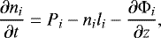 (1)
(1)
where Φi can be expressed as
 (2)
(2)
The variables ni, Pi, and li are the number density, volumic production rate, and volumic specific loss rate, and the altitude runs from −75 to 2800 km, with an altitude bin size of 5 km. The pressure levels covered in the model range from 5.3 bar to 1.05 × 10⁻⁷ mbar, and the 0 km altitude level is set at 1 bar.
The parameter Di is the molecular diffusion coefficient, T is the temperature, Hi and H are the individual and atmospheric scale heights, respectively, K(z) is the eddy diffusion coefficient, and αi is the thermal diffusion coefficient.
The equations are solved for H, He, methane (CH4), methyl radical (CH3), acetylene (C2H2), ethylene (C2H4), ethane (C2H6), methyl acetylene (CH3C2H), propene (C3H6), propane (C3H8), C3H2, C3H5, C3H7, diacetylene (C4H2), CH, C2, C4H, C3H5, C2H, 1CH2, 3CH2, C2H3, C2H5,  , C4H3, water (H2O), carbon monoxide (CO), carbon dioxide (CO2), methanol (CH3OH), CH2OH, CH3O, HCCO, CH3CO, C2H 4OH, molecular oxygen (O2), CH2CO, CH3CHO
  , formyl (HCO), formaldehyde (H2CO), hydroxyl (OH),
  ,
,  , CH3O, and CH3CO.
We use a fully implicit finite difference scheme (unconditionally stable) with a variable time step, Δ t, to accommodate the wide range of characteristic lifetimes (i.e. turbulent transport, molecular diffusion, and chemical) for every species. The abundance of every species at every atmospheric level is determined by the balance of photochemical and transport processes. If the computed number density ni due to theseprocesses is higher than the value allowed by the saturation law at the prevailing pressure and temperature at that level nis, i.e.  , then a condensation term is added to the photochemical loss. Lavvas et al. (2008a,b) recommend
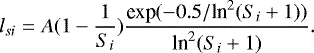 (3)
(3)
Here A is a constant in the range (0.1−1) × 10−7 s−1 as in Lavvas et al. (2008b) and Krasnopolsky (2009). The above expression provides increasing condensation loss rates with increasing saturation ratios Si. By varying the A values within the range given above, the resulting mixing ratio profiles below the condensation levels are noticeably affected, whereas at the pressure region where H2O and CO2 observations are available the resulting profiles differ only by 3–4%. Thus, we set A = 1 × 10⁻⁷ s−1, as Lavvas et al. (2008b) considered for Titan’s atmosphere.
At 5.3 bar, the lower boundary of our model computations, the condition is set as maximum downward velocity for every species except He and CO having constant mixing ratio (qCO = 5.0 × 10⁻¹⁰ as in Moses & Poppe 2017). For CH4, the mixing ratio is set to 1.0 × 10⁻⁵, which corresponds to its stratospheric value (Orton et al. 2014a; Lellouch et al. 2015). We note that we discard its condensation as it is unimportant for the study of the water, carbon monoxide, and dioxide stratospheric abundances.
At the upper boundary of the model placed at 1.05 × 10⁻⁷ mbar (or 2800 km above the 0 km altitude level placed at 1 bar), every species is in diffusive equilibrium (i.e. zero flux). Atomic hydrogen is injected in the atmosphere at a rate of 4 × 107 cm−2 s−1 (Moses et al. 2005) due to the photodissociation of H2 taking place above 1.05 × 10⁻⁷ mbar.
Our models are run for K(z) = 5000 cm2 s−1, as in Moses & Poppe (2017), for a better comparison of our results with theirs. Since our aim is to determine whether a cometary impact could have been responsible for the CO abundance observed today, once the size D of the impactor and the time of the event timpact are constrained, we will study how timpact varies as a function of K(z), for one particular D, to check whether it is compatible with estimates by Zahnle et al. (2003). We assume that the cometary material is delivered at a pressure level of 0.1 mbar (Lellouch et al. 1997, 2002). Model results for K(z) = 1200 cm2 s−1 (Cavalié et al. 2014)will be obtained and conclusions will be drawn.
The model, which was originally derived from González et al. (2011), has been adapted to the Uranus atmosphere by using the pressure−temperature profile in Orton et al. (2014a) shown in Fig. 1, considering a chemical network both for hydrocarbons and oxygen species derived from Moses et al. (2000a,b, 2005) and references therein. Some of the hydrocarbon reaction rates are updated as in Orton et al. (2014b) to allow for a more efficient recycling of C2H2, and we have also considered ethylene absorption cross sections measured at low temperatures by Wu et al. (2004). Comparisonof the column densities that best match the measurements by Spitzer (Orton et al. 2014b) and the values computed in this work can be seen in Table 1. For this comparison, we have set  at the lower boundary of the modelto 1.6 × 10⁻⁵, as in Orton et al. (2014b). On the other hand, the analysis of the oxygen species origin and abundance uses
 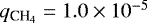 , as in Moses & Poppe (2017), for a more consistent comparison between our results and theirs. We note that this work does not focus on reproducing the hydrocarbon measurements, whose abundances derive from the chemistry initiated by methane photodissociation.
The hydrocarbon column densities obtained in this work vary by < 1% when the considered total oxygen steady influx is within the results given in Moses & Poppe (2017) (i.e. 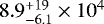 cm−2 s−1 oxygen atoms). This almost negligible difference is due to the strong depletion of hydrocarbons at p < 0.5 mbar, whereas ice grain ablation produces oxygen species at those pressure levels. Therefore, oxygen species and hydrocarbons are chemically decoupled. On the other hand, the column abundances of species listed in Table 1 show variations of ≤ 13% for the different cometary impact cases analysed in this work. As the CO delivered by the impactor at p ≤ 0.1 mbar is downward transported, it reaches atmospheric regions at the 0.2–1.0 mbar pressure level where methane abundance has not been considerablyreduced by diffusive separation. Hence, some chemical interaction between hydrocarbons and oxygen species develops. Nevertheless, these variations are within the error bars derived from Spitzer data and photochemical modelling.
The oxygen species chemical network considered in this work is given in Appendix A. It derives from Moses et al. (2000b). The H2O, CO, and CO2 abundance profiles are very little dependent on this network and on the hydrocarbon chemical reactions (see above), their vertical mixing ratio profiles being mostly determined by the influx of oxygen (steady or single event such as a cometary impact in the past) and the diffussion processes. This is so because low values of K(z) like those in the Uranus atmosphere result in methane homopause located at ~ 0.3–0.8 mbar; H2O and CO2 condense at relatively high atmospheric levels, and CO is highly stable, thus hydrocarbons and oxygen species turn out to be located in different stratospheric layers, and thus oxygen–carbon coupling chemistry can be considered unimportant.
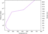 |
Fig. 1 Thermal vertical profile of the Uranus atmosphere from Orton et al. (2014a). |
Hydrocarbon column abundances at p < 10 mbar versus Spitzer observational results (Orton et al. 2014b).
3 Radiative transfer model
The Herschel CO spectra have been modelled with a line-by-line radiative transfer model, which takes into account the spherical geometry and broadening due to planetary rotation, developed for Jupiter (Moreno et al. 2001) and also used for Neptune (Moreno et al. 2017). The CO opacity parameters were taken from the Jet Propulsion Laboratory molecular line catalogue (Pickett et al. 1998); the collision-induced absorption opacity due to the main compounds of the Uranus atmosphere (H2 –H2, H2 –He, and H2 –CH4) adopt codes developed by Borysow et al. (1985, 1988) and Borysow & Frommhold (1986). We adopted a He mole fraction of 0.149 from Conrath et al. (1987), and the CH4 tropospheric value of 0.023 derived from Lindal et al. (1987). The Uranus thermal profile is from Orton et al. (2014a). The adopted CO pressure broadening coefficient γco(8−7) is 0.066 cm−1 atm−1, with a temperature dependance n = 0.64 (Sung 2004; Mantz et al. 2005). We note that the continuum level around the CO(8-7) line probes above ~ 0.6 bar pressure level.
4 Oxygen steady flux
By making use of our chemical network, treatment of condensation processes, and transport (turbulent and molecular diffusion), we first established the steady influx of H2O, CO, and CO2 needed for an overall agreement with the observations from ISO (Feuchtgruber et al. 1997), Herschel (Cavalié et al. 2014), and Spitzer (Orton et al. 2014b), respectively.
For an eddy diffusion coefficient K(z) = 5000 cm2 s−1, a productionrate profile (in molecules cm−3 s−1) of water, carbon monoxide, and carbon dioxide due to the ice grain ablation (Moses & Poppe 2017) is considered. We tune the integrated flux of each species to better match the available observations for every species. Table 2 lists the water and carbon dioxide fluxes needed in this work to obtain mixing ratios and column densities in good agreement with data. We have also run our model with the integrated ablation rates in Moses & Poppe (2017) for a comparison with their results. Figure 2 shows the mixing ratio profiles obtained in both models, TW18 and MP17, as well as the observational data. For the same influx of CO, 2.7 × 105 cm−2 s−1, our modelled carbon monoxide reproduces that of Moses & Poppe (2017) at p ≥ 0.1 mbar and at lower pressure slight discrepancies appear between TW18 and MP17.
However, the use of the integrated flux in Moses & Poppe (2017) for water and carbon dioxide (model MP17) gives rise to noticeably different mixing ratio values and column densities when compared to our computations in model TW18. More concisely, Moses & Poppe (2017) require twice the water influx we derive to match the observations (~ 4.4 × 10⁻⁹ at 0.03 mbar) and 50% less in the case of carbon dioxide. Regarding water, Fig. 3 clearly shows that at pressure lower than 0.015 mbar, our model MP17 computes a water mixing ratio profile that largely coincides with that in Moses & Poppe (2017). However, below this level the two profiles are noticeably different, ours overestimating the water abundance at 0.03 mbar by a factor of ~ 7 versus the ISO measurements. A mixing ratio in agreement with ISO observations can be achieved with a water integrated ablation rate of ~ 6.0 × 104 cm−2 s−1 (model TW18). Wehave also compared the theoretical water column density for water ablation rates 6.0 × 10⁴ and 1.2 × 105 cm−2 s−1 (model MP17) resulting in 4.3 × 10¹³ and 1.3 × 1014 cm−2, respectively, approximately within the range given by Feuchtgruber et al. (1997) (5− 12) × 1013 cm−2.
An important difference between models in Moses et al. (2000b) and this work is how condensation is included in the photochemical modelling. Moses et al. (2000b, 2005) follow a sophisticated condensation treatment where a vertical distribution of condensation nuclei and re-sublimation of ices are taken into account. We have considered a very simplified condensation scheme (see Eq. (3)). We note that the water profile derived in this work is highly supersaturated below the condensation level, whereas the profile in Moses & Poppe (2017) is undersaturated. The vapour pressure law used in this work is from Mauersberger & Krankowsky (2003):
 (4)
(4)
where the pressure P is in Pa, the temperature T is in K, the expression is valid in the region 165 < T < 273 K, and we assume it remains valid at lower temperatures. On the other hand, Moses & Poppe (2017) considered  (Marti & Mauersberger 1993). We have used this law in our model as well, and it does not account for the differences shown in Fig. 2. Since for the same water influx, the vertical mixing ratio profiles of water at p < 0.015 mbar in MP17 and TW18 coincide, we believe that condensation is the main driver of the discrepancies shown in Fig. 3. Thus, with current information about the water content in the Uranian atmosphere, the influx needed in this work and that in Moses & Poppe (2017) could both give rise to H2O mixing ratio profiles potentially reproducing the ISO observations. Comparison of ISO data with synthetic spectra generated with the theoretical water profiles obtained in this work would help to better determine the H2O influx.
We have also analysed why our modelling (TW18) requires 50% more carbon dioxide to match the Spitzer observations. Unlike the case of H2O where using the same influx as Moses & Poppe (2017) renders basically the same water vertical profile at p < 0.01 mbar (see Fig. 3), the computed carbon dioxide column abundance shows some dependency on the reaction rate for CO + OH → CO2 + H (k201 in Table A.1) in addition to the ice grain integrated flux. Table 3 shows the computed CO2 column density and mixing ratio varying both the integrated oxygen influx and the rate coefficient k201 (Moses et al. 2000b; Wakelam et al. 2012). The results indicate that a CO2 influx of 3.0 × 103 cm−2 s−1 (see row MP17 inTable 2), despite the k201, gives rise to carbon dioxide column abundances (6.9−7.6 × 10¹²) that are considerably below the Spitzer observations (1.7 ± 0.4 × 10¹³). Therefore, although the CO2 abundance slightly depends on k201, this cannot account for the large dissimilarity with Spitzer observations.
Obtaining the same results as in Moses & Poppe (2017) would require the use of exactly the same chemical network (reactions and their rate coefficients), which is beyond the scope of the current work. As the aim of this paper is to ascertain whether a cometary impact could be responsible for the current presence of oxygen species in the Uranus atmosphere, the conclusions on this open issue can be tackled regardless of the concise value of water and/or carbon dioxide integrated steady flux due to ice grain ablation. Nevertheless, the inconsistency between the required H2O influx in Moses & Poppe (2017) and in these computations with respect to the ISO observations is only ~ 50%, well within the observational errors.
Comparison of theoretical results with available observations versus the integrated flux of oxygen due to ice grain ablation.
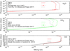 |
Fig. 2 H2O, CO2 and CO vertical profiles obtained with steady ablation rates in models TW18 and MP17 compared with available ISO, Spitzer and Herschel observations. Best-fit profiles from Moses & Poppe (2017) are also shown for comparison. |
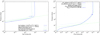 |
Fig. 3 Comparison of the H2O and CO2 profiles obtained in models TW18 and MP17, with ISO (Feuchtgruber et al. 1997) and Spitzer observations (Orton et al. 2014b), respectively. Best fits in Moses & Poppe (2017) are also shown. |
5 Cometary impact as the only oxygen source
In this section we explore in detail whether the time evolution of the material (mostly CO and H2O) delivered by a cometary impact could be responsible for the observed abundances of these species. Cavalié et al. (2014) and Moses & Poppe (2017) mention in their works that a cometary source of CO is not an unexpected possibility for Uranus, supplying an external amount of oxygen that is of the same magnitude as the dust influx (Poppe 2016).
We first considered that a cometary impact brought the currently observed carbon monoxide; that is to say, CO did not diffuse upwards from deep atmospheric levels. As in Moreno et al. (2012) and Lara et al. (2014) and references therein, we assume that this cometary impact behaves like that of Jupiter/Shoemaker–Levy 9 where the cometary oxygen ended up as CO and H2O during the shock chemistry at plume re-entry near the 0.1 mbar and lower pressure levels, and both species have since then slowly diffused vertically. No CO2 was produced in this shock chemistry.
Following Cavalié et al. (2014), discarding CO photochemical processes, that is, using a purely diffusive model with K(z) = 1200 cm2 s−1, considering that a comet of 640 m diameter (i.e. 9.3 × 10¹⁵ CO molecules cm−2 or 3.5 × 10¹³ g were produced by the cometary impact in the Uranus atmosphere) hit the planet 370 yr ago, our CO mixing ratio profile perfectly matches that in Fig. 2 of Cavalié et al. (2014). These results validate both diffusion models.
Our work then focused on determining the impactor size (diameter D in km) and when it occurred (timpact yr ago) in order to obtain a CO mixing ratio whose synthetic spectrum matches the Herschel observations (Cavalié et al. 2014) and qCO < 2.0 × 10⁻⁹ in the 200–100 mbar range (Teanby & Irwin 2013). For this modelling, we fixed the eddy diffusion coefficient to our nominal value of K(z) = 5000 cm2 s−1.
To determine which stratospheric CO mixing ratio best matches the observations, as a starting point, we arbitrarily considered an impactor of 2 km in diameter and let the system evolve over several hundred years (i.e. to determine when the impact happened, timpact) to obtain several qCO profiles that are used as input in the sub-mm radiative transfer computations (see Sect. 3). Aiming for a realistic study, we allowed chemistry to distribute the oxygen influx among the different species considered in the model (see Sect. 2). For those species whose resulting partial pressure is higher than that allowed by the vapour pressure law, an additional term loss due to condensation is considered following Eq. (3).
The outcome of this sensitivity test indicates that a CO relative abundance of 7.0 × 10⁻⁹ at 0.4 mbar allows an optimal match of the line core and wings. Table 4 lists different cases where (D, timpact) have been tuned to obtain qCO = (7.0 ± 0.1) × 10−9 at the ~0.4 mbar region, the delivered CO mass (in g), and the CO mixing ratio obtained in 200–100 mbar. The resulting profiles in the 200–100 mbar region reflect that larger impactors give rise to larger CO abundances although below the upper limits in Teanby & Irwin (2013). Table 4 shows that the solution is degenerate; in other words, the same stratospheric CO mixing ratio abundance can be obtanied with pairs of (D, timpact) that represent larger impacts having taken place longer ago, or smaller impactors occurred more recently. For instance, the temporal evolution of the material delivered by a cometary impact indicates that the CO currently observed in the Uranus stratosphere could be due to a comet nucleus of 3.5 km diameter that hit the planet 822 yr ago.
Figure 4 shows the comparison of the measured spectra and the modelled radiative transfer as a function of the different CO vertical distribution resulting from steady ice grain ablation and cases 3 and 4 for cometary impact. Any other of the cases in Table 4 will give rise to a CO mixing ratio of ~ 7.0 × 10⁻⁹ at the 0.4 mbar pressure level that will give good match to the Herschel data. Stratospheric CO mixing ratio profiles with an abundance larger than the value in the pressure range probed by Herschel (i.e. between 3 and 0.4 mbar) can in principle be discarded as they will overestimate the observations. Similarly, the tropospheric CO mixing ratio profile has to be lower than the upper limit 2.1 × 10⁻⁹ established by Teanby & Irwin (2013).
Equations (14) and (15) in Zahnle et al. (2003), adapted to Uranus where the impact frequency is ~ 4 times smaller than on Jupiter, allow us to plot the frequency of impact versus the impactor size. Figure 5 displays two different scenarios depending on the origin of the impactors: the size-number distribution of impactors is like that inferred at Jupiter (ecliptic comets), and those impactors more representative of nearly isotropic comets (as long-period or Halley-type comets). Zahnle et al. (2003) conclude that known craters on the Saturnian and Uranian satellites are consistent with either case; that is, both kinds of impactors are in the Uranian system and they could have entered the Uranus atmosphere. Also, Zahnle et al. (2003) assume that the impact rate on Uranus is ~ 0.00125 comets per year (i.e. one impact every ~800 yr) with D > 1.5 km with an uncertainty to a factor of 6. Hence, to constrain the most likely size of the impactor and time, (D, timpact), that could be responsible for the CO in the Uranian stratosphere, we can follow two approaches: (i) either we consider that one impact takes place every ~ 800 yr, the size of the impactor being D > 1.5 km, and this is fulfilled in cases 4, 5, and 6 (and every other case where D and timpact are larger with the only constraint that the tropospheric CO mixing ratio remains below the upper limit in Teanby & Irwin 2013), or (ii) we distinguish the two types of impactors–those at ecliptic orbits (known as Uranus A), or those in nearly isotropic orbits (known as Uranus B) – to assess the origin of the impactor on the planet and the subsequent shock chemistry that gave rise to the currently detected CO. In the latter consideration, impactors with ~ 1 < D < 2 km and ~ 450 < timpact < 630 yr are in the range allowed by the curves in Fig. 5.
The cometary impact delivers 10 times less H2O than CO, and no CO2. The resulting water and carbon dioxide profiles for cometary impacts pertaining to cases 0–3 in Table 4 are shown in Fig. 6 together with ISO and Spitzer measurements.
As most of the oxygen released by a shock chemistry induced during the cometary impact is in the form of CO (90%) and H2O (10%), the only source of CO2 is subsequent oxygen chemistry. The process CO + OH → CO2 + H produces negligible amounts of CO2 as the abundance of the reactants is very low at the p < 0.5 mbar once the evolution time is such that CO stratospheric mixing ratio matches the Herschel data and H2O is highly reduced in the upper atmosphere where its photolysis gives rise to OH. The resulting CO2 integrated column densities range from 3.9 × 10¹⁰ to 2.4 × 1011 cm−2 for the cases in Table 4, clearly well below the Spitzer measurements (Orton et al. 2014b) (1.7 ± 0.4 × 10¹³). Similarly, our computed mixing ratio is considerably lower than 8 × 10⁻¹¹ in Orton et al. (2014b).
Feuchtgruber et al. (1997) derived a relative abundace of 6− 14 × 10−9 at p < 0.03 mbar. The cometary impact delivers the CO and H2O at p < 0.1 mbar (Lellouch et al. 2005). The H2O profile resulting from the time evolution of the water delivered by a cometary impact is noticeably below the ISO observations (see Fig. 6). The H2O rapidly dissociates given the poor UV shielding by hydrocarbons absorbing at the same wavelengths as water does, and it is rapidly transported downwards as condensation represents the most important sink for this species between 3.1 bar and 2.6 mbar. The gaseous water deposited by the impact diffuses downward to the 0.03 mbar region to give a mixing ratio of 6− 14 × 10−9 in only ~ 50 yr. In that time lapse, CO abundance at ~0.4 mbar is orders of magnitude higher than ~7.0 × 10⁻⁹ as it takes centuries to diffuse to the atmospheric region where Herschel has detected it (Cavalié et al. 2014). Figure 7displays thewater, carbon monoxide, and carbon dioxide profiles obtained for impactors of 1.6 and 2.0 km diameter. The evolution time is set to ~ 50 yr, which provides an H2O mixing ratio matching the ISO observations. However, the carbon monoxide and carbon dioxide noticeably overestimate the Herschel and Spitzer measurements, respectively.
From this analysis, we can conclude that the current CO stratospheric abundance can derive from a cometary impact that occurred several centuries ago, whereas the observed water and carbon dioxide observed mixing ratios cannot be explained by this event alone. In summary, from the modelling presented in this section, we can discard a single cometary impact as the only origin of the current stratospheric H2O and CO2 measured abundances, whereas CO best fit to Herschel observations can be obtained if a comet of ~ 1.2–2.0 km diameter impacted the planet ~450–630 yr ago, or a large impact (D ~ 3.5 km) took place ~800 yr ago.
Considering an eddy diffusion coefficient K(z) = 1200 cm2 s−1 (as in Cavalié et al. 2014) and assuming that the shock chemistry produces CO at the 0.1 mbar level, the diffusion times needed to reach qCO ~ 7.0 × 10⁻⁹ at 0.4 mbarare considerably longer than the values listed in Table 4. More concisely, for D = 1.6 km, the diffusion time is ~900 yr, whereas for D = 3.5 km, timpact ~ 1600 yr ago. In principle, these old impacts cannot be discarded according to Zahnle et al. (2003). However, the CO stratospheric profiles render synthetic spectra that are more intense and broader than the observed spectrum. Nevertheless, decreasing the CO abundance by 40%, the resulting profile can fit the Herschel observations (see Fig. 4).
CO2 column density and mixing ratio obtained for several oxygen influx and CO+OH → CO2 + H reaction rate coefficients.
Impactor size and time to reproduce CO available observations and upper limit, respectively (Cavalié et al. 2014; Teanby & Irwin 2013).
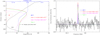 |
Fig. 4 Comparison of the CO line observed with Herschel and the spectra computed with the resulting CO vertical profile pertaining to model MP17, nominal case 3 (K(z) = 5000 cm2 s−1), 40% of qCO resulting from case 3 with K(z) = 1200 cm2 s−1, and case 4 in Table 4. WF denotes the weighting function at the line centre. |
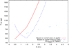 |
Fig. 5 Inverse of the impact frequency (in units of years ago) versus impactor size D on Uranus for two different scenarios: impactors in which the size–number distribution of impactors represent ecliptic comets (red solid line), and nearly isotropic comets such as long-period and Halley-type comets (blue dashed line; see Zahnle et al. 2003, and references therein). Stars show the (D, timpact) from Table 4 that allows for an optimal match of Herschel CO data in the stratosphere and below the upper limit in the troposphere (Teanby & Irwin 2013). |
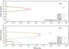 |
Fig. 6 Vertical profiles of H2O and CO2 derived from the time-dependent model assuming three different scenarios for a cometary impact on Uranus (cases 0–3 in Table 4) delivering 10 times less H2 O than CO, and no CO2. Available observational data on H2O (Feuchtgruber et al. 1997) and best-fit |

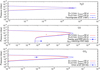 |
Fig. 7 Mixing ratio profiles of H2O, CO, and CO2 ~ 50 yr after a comet nucleus of size 1.6 and 2.0 km impacted Uranus. The evolution time is tuned to reproduce the water ISO observations, which in turn produces carbon monoxide and carbon dioxide clearly above the available measurements. Photochemical, condensation, turbulent transport with K(z) =5000 cm2 s−1, and molecular diffusion are taken into account. |
6 Combined oxygen source: meteoroid ablation and cometary impact
The best-fit model to CO, H2O, and CO2 by Moses & Poppe (2017) requires a total oxygen influx rate that is a factor of 4 higher than original predictions from the ablation of ice grains (4.0 × 10⁵ versus 8.9 × 104 cm−2 s−1). They give different arguments to explain the origin of this mismatch, for example uncertainties in the ablation modelling or additional external sources of oxygen to Uranus, such as satellite/ring debris or cometary impact. In this section, we analyse whether a combined source of oxygen entering the Uranus atmosphere can reproduce the water, carbon monoxide, and carbon dioxide observations.
6.1 H2O and CO2 steady source and CO of cometary origin
This scenario contemplates a combined source in which water is mainly produced by the injection rate (in molecules cm−3 s−1) shown in Fig. 6 of Moses & Poppe (2017) due to the ablation of ice grains. We considered an H2O integrated ablation rate of 6.0 × 104 cm−2 s−1 because in our study, and for the case of a steady oxygen source, it is the best value that reproduces the ISO observations (Feuchtgruber et al. 1997; see Sect. 4). The gas−gas chemistry contemplated in our chemical scheme gives contributes very little to the overall production of water. On the other hand, carbon monoxide and water originate from a cometary impact in a ratio of 90:10. In this line, we have arbitrarily chosen case 3 in Table 4 (D = 2.0 km, timpact = 630 yr ago). We note that any other cometary impact case studied in Sect. 5 leads to the same general conclusions. The upper panel of Fig. 8 displays the results of this combined source of oxygen entering the Uranus atmosphere. As expected, the predicted CO and H2O perfectly match the observations, but carbon dioxide is severely underestimated: the reaction R201 (CO + OH → CO2 + H) cannot efficiently proceed as the two involved reactants are present at different atmospheric regions. This makes the CO2 production very inefficient. Additionally, carbon dioxide irreversibly condenses between 410 and 7 mbar. The measured column density of CO2 by Spitzer can be achieved by considering a carbon dioxide integrated external flux of 4.5 × 103 cm−2 s−1 due to ice grain ablation (lower panel in Fig. 8). In this way, the currently available set of water, carbon monoxide, and carbon dioxide observations can be reproduced by invoking a cometary impact ~ 630 yr ago bringing 1.1 × 10¹⁵ gr of CO, and an external steady source of 4.5 × 10³ and 6.0 × 104 cm−2 s−1 of CO2 and H2O, respectively.
6.2 Steady source of H2O, CO, and CO2, and cometary impact delivering CO
We also studied a combined CO source, namely carbon monoxide produced by a cometary impact as well as an oxygen steady source due to ice grain ablation that also injects water and carbon dioxide into the Uranus atmosphere. From a physical point of view there is no reason to discard such a scenario. Models are run by fixing the water and the carbon dioxide steady influx to the values needed to match current observations (see above and Sect. 4), 6.0 × 10⁴ and 4.5 × 103 cm−2 s−1, respectively. Thus, assuming as a total oxygen influx the nominal result in Moses & Poppe (2017) (8.9 × 104 cm−2 s−1), carbon monoxide has to be produced by ice grain ablation at a rate of 2.45× 104 cm−2 s−1. This gives the following relative influx rates 67% H2O, 28% CO, and 5% CO2. In addition to this CO influx, we consider that a comet nucleus of ~ 2 km (case 3 in Table 4) impacted the planet. After 639 yr the stratospheric carbon monoxide abundance allows for a good match of Herschel measurements, as shown in Fig. 9. The resulting CO vertical profile in the pressure range p > 0.05 mbar reflects the downward-transported carbon dioxide over 639 yr, whereas at lower pressures the vertical profile reflects the steady influx.
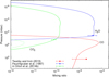 |
Fig. 8 Vertical profiles of H2O, CO, and CO2 derived fromthe time-dependent model under these assumptions: (i) 1.1 × 10¹⁵ gr of CO are brought to the planet via a cometary impact ~630 yr ago (case 3 in Table 4), and (ii) vapour water input is due to the ablation of ice grains (Moses & Poppe 2017) with an integrated rate of 6.0 × 104 cm−2 s−1. Red solid line: CO, blue solid line: H2O, dashed green line: CO2 only produced by chemical processes, and green solid line: carbon dioxide when an integrated ice grain ablation rate of 4.5 × 104 cm−2 s−1 is considered as well. |
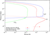 |
Fig. 9 Mixing ratio profiles of H2O, CO, and CO2 obtained when a production rate due to ice grain ablation for every species with integrated rates of 6.0 × 10⁴, 2.45 × 10⁴ and 4.5 × 103 cm−2 s−1 is taken into account. An additional source of cometary CO is considered as well, the impactor size is D = 2 km, and the evolution time needed to match the Herschel observations is 639 yr. The red dashed line refers to the carbon monoxide profile resulting from the simulation of case 2 (see Table 4). |
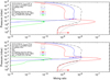 |
Fig. 10 Mixing ratio profiles of the most abundant oxygen species in the Uranus atmosphere assuming an oxygen combined source due to ice grain ablation and cometary impact. Upper panel: mixing ratio profiles resulting from assuming H2 O and CO influx of 6.0 × 10⁴ and 2.9 × 104 cm−2 s−1, respectively. Additionally, an impactor of 0.64 km in diameter hits the planet delivering only CO (see Table 4). Carbon dioxide is produced by chemical reactions. The evolution time of the material delivered by the comet is tuned to produce a CO2 abundance compatible with Spitzer observations resulting into timpact = 67 yr. On the other hand, CO largely overestimates the data. Lower panel: as above, but the size of the impactor is reduced to 0.56 km to inject a smaller amount of CO in the atmosphere. The evolution time needed to match the CO2 observationsis 19 yr giving rise to a CO mixing ratio ~5 × 10⁻⁹ at 0.4 mbar, whereas H2O largely overestimates ISO data. |
6.3 Steady source of H2O and CO, and cometary impact delivering CO
Another possible scenario is to assume that only water and carbon monoxide are produced during the ice grain ablation with influxes of 6.0 × 10⁴ and 2.9 × 104 cm−2 s−1, respectively. The total oxygen influx is thus the nominal result in Moses & Poppe (2017), 8.9 × 104 cm−2 s−1. The carbon dioxide chemical production in this model run, i.e. no external source of CO2, does not give rise to its measured abundance. Therefore, our aim is to match the CO2 observations by determining when an impactor collided with the planet delivering CO and H2O in the usual proportion (90:10) so that CO2 could attainthe observed mixing ratio. As an example, we consider case 0 in Table 4, D = 0.64 km, 3.5 × 10¹³ gr of CO delivered to the planet and CO2 only produced by the chemical reaction CO + OH → CO2 + H. After 67 yr of chemical and dynamical evolution, the CO2 stratospheric mixing ratio coincides with the value derived from the Spitzer observations. However, the profile that matches the Spitzer observations more closely according to Orton et al. (2014b) is dramatically different from that obtained in this simulation. These photochemical models alone cannot conclude whether the carbon dioxide profile shown in the lower panel of Fig. 10 agrees with Spitzer data. Synthetic spectra should be computed and compared with observational data, and this is beyond the scope of the current paper. Whereas CO2 might reproduce the observations (with the caveats noted above), the CO abundance at 0.4 mbar is one order of magnitude larger than Herschel data indicate (see upper panel in Fig. 10). Given the degeneracy noted in Sect. 5, larger impacts should have taken place longer ago; however, they are not favoured as the stratospheric CO would considerably exceed the measurements. In order to have a stratospheric CO mixing ratio of ~ 7.0 × 10⁻⁹ at 0.4 mbar, the impactor size has to be smaller (D = 0.56 km) and the event has to have occurred only 19 yr ago. This scenario is fatal for the computed H2O abundance as it surpasses the measurements by a factor of 10 (see lower panel in Fig. 10). We note that the water diffusion time is ~ 60 yr, and the evolution time requested in this simulation to obtain CO and CO2 mixing ratios in agreement with observations is only 20 yr. In both of these cases, although the stratospheric CO2 mixing ratio agrees with the value that Orton et al. (2014b) consider their best fit, the column densities are a factor of 2 below the Spitzer measurements.
7 HCN as diagnostic of CO origin
The Shoemaker−Levy 9 impact on Jupiter in July 1994 evidenced the delivery of other minor species of cometary origin in addition to CO (Lellouch et al. 1995). Bézard et al. (1997) was able to detect emission from hydrogen cyanide over all the impact sites they observed with the NASA Infrared Telescope Facility. The total mass of HCN delivered by the SL9 impact was 1.1 ± 0.4 × 10¹³ g. On the other hand, the total mass of CO was estimated to be 1.5 ± 0.6 × 10¹⁵ g (Lellouch et al. 1997). This gives a mass ratio CO/HCN ~ 100 for the material delivered by the cometary impact.
In our modelling, we assume that the hypothetical comet that could have impacted on Uranus injected hydrogen cyanide into the planet’s atmosphere as 1% of the carbon monoxide (in mass) at pressure levels p ≤ 0.1 mbar. Once in the atmosphere, HCN is subjected to eddy and molecular diffusion, condensation, and photochemical processes.
As an exploratory work, we first ran a pure diffusive model (hydrogen cyanide does not undergo either photochemistry or condensation) in which an impactor of 0.64 km diameter hit the planet 250 yr ago (case 0 in Table 4). Figure 11 shows the CO and HCN resulting profiles. As expected, carbon monoxide reproduced the Herschel observations in the stratosphere, and the hydrogen cyanide mixing ratio is ~ 100 times lower than that of CO: qHCN ~ 5.0 × 10⁻¹¹. Since the molecular mass of CO and HCN are very similar, diffusive separation acts similarly on both species at low pressures. On the other hand, at higher pressures, carbon monoxide and hydrogen cyanide mixing ratio profiles considerably differ due to the lower boundary condition imposed on HCN (maximum downward flux) and on CO (constant mixing ratio at 5.0 × 10⁻¹⁰).
Aiming for a more realistic model, we also considered that hydrogen cyanide suffers photodissociation and condensation, whereas chemical recycling is not considered in this work. Therefore, in this work HCN is irreversibly lost by photodissociation in the upper atmosphere and condensation in the ~ 140−2 mbar region where the abundance drastically decreases to very low mixing ratios. For three different cometary impact scenarios (cases 0, 2, and 3 in Table 4), the model results are shown in Fig. 11. The hydrogen cyanide mixing ratio is ≤ 3.0 × 10⁻¹⁷ at the 0.5 mbar pressure level, undetectable from ground with ALMA (T. Cavalié, priv. comm.). More recent impacts (and thus, smaller impactors than the ones in Table 4) give rise to a higher concentration of hydrogen cyanide in the stratosphere, whereas older events produce broader HCN profiles peaking at much lower mixing ratio values.
To assess the importance of the chemical production of HCN, we have studied likely sources involving nitrogen species such as N2 and NH3. For this, we ran a thermochemical model with the (p,T) profile from Fig. 3 in Cavalié et al. (2014) and the same O/H and C/H values (501 and 18 times the solar value), and N/H solar value. The obtained NH3 molar fraction is ~10−4 from ~104 bar up to 3.2 bar. Ammonia condenses considerably below the tropopause, thus it cannot initiate gaseous chemistry above this level. The N2 molar fraction smoothly decreases with decreasing pressure from ~10−7 at ~104 bar to ~ 10−16 at 80 bar. For Kzz = 108 cm2 s−1 as in Cavalié et al. (2014), the N2 quenching level might be between 2000 and 3000 bar, hence at lower pressure levels, molecular nitrogen should have a fairly (and low) constant mixing ratio of ~10−8. However, Fegley & Prinn (1986) concluded that their thermochemical equilibrium calculations (for a model enriched 500 times relative to solar abundances) predict that N2 is the most abundant non-equilibrium trace gas which can be mixed upward from the deep atmosphere of Uranus yielding 130 ppmv (1.3 × 10⁻⁴) for an eddy diffusion coefficient in the range 107 –108 cm2 s−1. Conrath et al. (1993) estimated N2 could be as high as 0.3–0.6% in Neptune and thus, similar to Uranus if the He mixing ratio is 0.15 for both planets. For an enrichment of nitrogen 500 times the solar value and Kzz= 108 cm2 s−1, our thermochemical model predicts a molecular nitrogen mixing ratio ranging from ~ 3% at p > 700 mbar and ~7% at lower pressures. In either case, it might well be possible that galactic cosmic rays (GCR) that impact on N2 can initiate an effective nitrogen chemistry (see e.g. Table II in Lellouch et al. 1994) able to steadily produce HCN. We leave the inclusion of nitrogen chemistry in the Uranus atmosphere for a future paper.
A comparison of the likely HCN abundance in the Uranus atmosphere and that detected in the atmospheres of Neptune and Jupiter is also very instructive. In Neptune’s atmosphere, in addition to the cometary impact delivering HCN, there might be chemical sources forming HCN which would allow for a higher stratospheric abundance versus the scenario where HCN only originates from a cometary impact and is lost by photolysis and condensation. Lellouch et al. (1994, 2005) took into account chemical formation processes for HCN: nitrogen atoms escaping Triton and entering Neptune’s upper atmosphere, and N2 dissociation by galactic cosmic ray impact reaching deep atmospheric levels. In addition to this, Neptune orbits the Sun at ~ 30 AU (versus ~19 AU for Uranus) causing a lower radiation flux reaching the planet. Additionally, the methane abundance is two orders of magnitude higher in Neptune’s atmosphere than in the Uranus atmosphere; the homopause in Neptune’s atmosphere is at lower pressure levels than in that of Uranus; methane and the C2, C3, and C4 hydrocarbons can absorb most of the UV solar radiation high in the stratosphere shielding the photolysis of other very minor species. As a conclusion, HCN photodissociation on Neptune proceeds at a much slower rate than on Uranus.
Regarding HCN in Jupiter’s atmosphere, we note that although Jupiter receives a much higher UV solar flux (orbit of the planet at 5.2 AU from the Sun), the methane and hydrocarbon abundances are considerably higher at Jupiter than at Uranus, and the Jovian hompause is at ~10−4 mbar at much higher levels than on Uranus. Thus, the HCN photochemical lifetime in Jupiter’s atmosphere is much longer than in the Uranus atmosphere.
This work leads us to conclude that, unless HCN is chemically formed, once produced by the cometary impact, it is irreversibly destroyed resulting in barely detectable abundances in the stratosphere. A larger comet nucleus impacting the planet (i.e. more HCN injected in the atmosphere) does not alleviate the problem as the evolution time has to be longer to match the measured CO giving rise to a drastic depletion of HCN.
Detecting and measuring the HCN abundance could help to provide a further constraint on the origin of carbon monoxide in the Uranus atmosphere. A non-detection, placing an upper limit on the HCN abundance, would be also valuable to constrain (D, timpact). Hence, the hydrogen cyanide abundance predicted in this work is a worst-case scenario and it has to be regarded with caution.
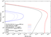 |
Fig. 11 CO and HCN mixing ratio profiles assuming both species are delivered by a cometary impact with parameters (D, timpact) as indicated. The resulting CO profiles match the Herschel observations. |
8 Conclusions
The different scenarios analysed in this work that allow for a good match to current observations of water, carbon monoxide, and carbon dioxide in the Uranus atmosphere are shown in Table 5.
The available observations of H2O, CO, and CO2 can be fit by assuming that these oxygen-bearing species are solely produced by ice grain ablation, as shown in Moses & Poppe (2017), with an influx rate of 3.75 × 105 cm−2 s−1 (see first row in Table 5).
Developing time-dependent photochemical models in which the currently observed atmospheric CO is delivered by a cometary impact alone, we were able to constrain the size (in km) of the impact and when it could have taken place. Our results indicate that impactors D ≤ 3.5 km ocurring timpact ≤ 822 yr give rise to CO in agreement with observations, and are compatible with the impact rates at Uranus shown in Zahnle et al. (2003). Whereas the cometary CO allows us to reproduce the observations, the cometary H2O renders stratospheric abundances much lower than ISO data due to a much shorter lifetime than that of CO, being necessary a steady influx of water to match ISO observations. Similarly, the scenario of CO and H2O originated from an impact (mass ratio of 90:10) fails to chemically produce enough CO2. A combinedsource of external oxygen (i.e. CO due to a cometary impact and/or ice grain ablation, and H2O and CO2 supplied from ice grain ablation) provides a good fit to the measured abundances of these three species. Current carbon monoxide observations (Cavalié et al. 2014) do no allow us to discriminate between the three analysed scenarios, namely oxygen-bearing species supplied by cometary origin, by ice grain ablation, or both. The CO vertical mixing ratio profile shows a very different shape when due to the ablation of ice grains, to cometary impact, or to a combinationof the two (see Fig. 17 in Moses & Poppe 2017, and Figs. 8 and 9in this work). Regarding water and carbon dioxide, we can conclude that a cometary impact is not the only cause of thecurrent abundance of these species in the Uranus atmosphere; instead, a steady source has to be invoked.
Ideally, observations whose analysis retrieve vertical profiles could provide the answer to the open question of the oxygen origin in the Uranus atmosphere. Another approach to shed light on this open question could be the search for trace species, for example HCN, as the aftermath of the collision of a comet on Uranus. A simulation of the temporal evolution of cometary HCN indicates that, once deposited at p ≤ 0.1 mbar and in the absence of nitrogen chemistry, its photodissociation and condensation decrease its abundance to almost undetectable levels by current ground-based facilities as ALMA. Chemical hydrogen cyanide recycling initiated by GCR impact on N2 could give rise to much higher, and thus detectable, HCN stratospheric abundance.
Fit(Y/N) to current H2O, CO, and CO2 observations with models developed in this work.
Acknowledgements
This research has been supported by the Spanish Ministerio de Economía y Competitividad under contracts ESP2014–54062–R and ESP 2016–76076–R. L.M.L. wishes to express her gratitude to the International Space Science Institute (atBern, Switzerland) for supporting her research in the framework of the Visiting Science Program. M.L. acknowledges the Agencia Estatal de Investigación for the BES–2015–074542 fellowship co-funded by the Fondo Social Europeo. We are very grateful to the reviewer, Dr T. Cavalié, for the detailed comments which have considerably improved the manuscript.
Appendix A List of chemical reactions
Here we list the chemical reactions coupling oxygen species and hydrocarbons. The models were also run considering the hydrocarbon−hydrocarbon reactions not listed here. The numbering of the reactions reflects the complete set of considered reactions, listing here only those involving oxygen species. All values are quoted in the cm s system. Three-body reaction rates are computed according to the expression k = (k0k∞)∕(k0M + k∞), where M denotes the total number density.
C–H–O reactions.
References
- Bézard, B., Griffith, C. A., Kelly, D. M., et al. 1997, Icarus, 125, 94 [NASA ADS] [CrossRef] [Google Scholar]
- Borysow, A., & Frommhold, L. 1986, ApJ, 304, 849 [NASA ADS] [CrossRef] [Google Scholar]
- Borysow, J., Trafton, L., Frommhold, L., & Birnbaum, G. 1985, ApJ, 296, 644 [NASA ADS] [CrossRef] [Google Scholar]
- Borysow, J., Frommhold, L., & Birnbaum, G. 1988, ApJ, 326, 509 [NASA ADS] [CrossRef] [Google Scholar]
- Cavalié, T., Billebaud, F., Dobrijevic, M., et al. 2009, Icarus, 203, 531 [NASA ADS] [CrossRef] [Google Scholar]
- Cavalié, T., Hartogh, P., Billebaud, F., et al. 2010, A&A, 510, A88 [NASA ADS] [CrossRef] [EDP Sciences] [Google Scholar]
- Cavalié, T., Feuchtgruber, H., Lellouch, E., et al. 2013, A&A, 553, A21 [NASA ADS] [CrossRef] [EDP Sciences] [Google Scholar]
- Cavalié, T., Moreno, R., Lellouch, E., et al. 2014, A&A, 562, A33 [NASA ADS] [CrossRef] [EDP Sciences] [Google Scholar]
- Conrath, B., Gautier, D., Hanel, R., Lindal, G., & Marten, A. 1987, J. Geophys. Res., 92, 15003 [NASA ADS] [CrossRef] [Google Scholar]
- Conrath, B. J., Gautier, D., Owen, T. C., & Samuelson, R. E. 1993, Icarus, 101, 168 [NASA ADS] [CrossRef] [Google Scholar]
- Fegley, Jr., B., & Prinn, R. G. 1986, ApJ, 307, 852 [NASA ADS] [CrossRef] [Google Scholar]
- Feuchtgruber, H., Lellouch, E., de Graauw, T., et al. 1997, Nature, 389, 159 [NASA ADS] [CrossRef] [PubMed] [Google Scholar]
- Fletcher, L. N., Swinyard, B., Salji, C., et al. 2012, A&A, 539, A44 [Google Scholar]
- González, A., Hartogh, P., & Lara, L. M. 2011, Adv. Geosci., 25, 209 [Google Scholar]
- Krasnopolsky, V. A. 2009, Icarus, 201, 226 [NASA ADS] [CrossRef] [Google Scholar]
- Lara, L. M., Lellouch, E., González, M., Moreno, R., & Rengel, M. 2014, A&A, 566, A143 [Google Scholar]
- Lavvas, P. P., Coustenis, A., & Vardavas, I. M. 2008a, Planet. Space Sci., 56, 27 [NASA ADS] [CrossRef] [Google Scholar]
- Lavvas, P. P., Coustenis, A., & Vardavas, I. M. 2008b, Planet. Space Sci., 56, 67 [NASA ADS] [CrossRef] [Google Scholar]
- Lellouch, E., Romani, P. N., & Rosenqvist, J. 1994, Icarus, 108, 112 [NASA ADS] [CrossRef] [Google Scholar]
- Lellouch, E., Paubert, G., Moreno, R., et al. 1995, Nature, 373, 592 [NASA ADS] [CrossRef] [PubMed] [Google Scholar]
- Lellouch, E., Bézard, B., Moreno, R., et al. 1997, Planet. Space Sci., 45, 1203 [NASA ADS] [CrossRef] [Google Scholar]
- Lellouch, E., Bézard, B., Moses, J. I., et al. 2002, Icarus, 159, 112 [NASA ADS] [CrossRef] [Google Scholar]
- Lellouch, E., Moreno, R., & Paubert, G. 2005, A&A, 430, L37 [NASA ADS] [CrossRef] [EDP Sciences] [Google Scholar]
- Lellouch, E., Hartogh, P., Feuchtgruber, H., et al. 2010, A&A, 518, L152 [NASA ADS] [CrossRef] [EDP Sciences] [Google Scholar]
- Lellouch, E., Moreno, R., Orton, G. S., et al. 2015, A&A, 579, A121 [NASA ADS] [CrossRef] [EDP Sciences] [Google Scholar]
- Lindal, G. F., Lyons, J. R., Sweetnam, D. N., et al. 1987, J. Geophys. Res., 92, 14987 [NASA ADS] [CrossRef] [Google Scholar]
- Mantz, A. W., Malathy Devi, V., Chris Benner, D., et al. 2005, J. Mol. Struct., 742, 99 [NASA ADS] [CrossRef] [Google Scholar]
- Marti, J., & Mauersberger, K. 1993, Geophys. Res. Lett., 20, 363 [NASA ADS] [CrossRef] [Google Scholar]
- Mauersberger, K., & Krankowsky, D. 2003, Geophys. Res. Lett., 30, 1121 [NASA ADS] [CrossRef] [Google Scholar]
- Moreno, R., Marten, A., Biraud, Y., et al. 2001, Planet. Space Sci., 49, 473 [NASA ADS] [CrossRef] [Google Scholar]
- Moreno, R., Lellouch, E., Lara, L. M., et al. 2012, Icarus, 221, 753 [NASA ADS] [CrossRef] [Google Scholar]
- Moreno, R., Lellouch, E., Cavalié, T., & Moullet, A. 2017, A&A, 608, L5 [NASA ADS] [CrossRef] [EDP Sciences] [Google Scholar]
- Moses, J. I., & Poppe, A. R. 2017, Icarus, 297, 33 [NASA ADS] [CrossRef] [Google Scholar]
- Moses, J. I., Bézard, B., Lellouch, E., et al. 2000a, Icarus, 143, 244 [NASA ADS] [CrossRef] [Google Scholar]
- Moses, J. I., Lellouch, E., Bézard, B., et al. 2000b, Icarus, 145, 166 [NASA ADS] [CrossRef] [Google Scholar]
- Moses, J. I., Fouchet, T., Bézard, B., et al. 2005, J. Geophys. Res. Planets, 110, 8001 [NASA ADS] [CrossRef] [Google Scholar]
- Orton, G. S., Fletcher, L. N., Moses, J. I., et al. 2014a, Icarus, 243, 494 [NASA ADS] [CrossRef] [Google Scholar]
- Orton, G. S., Moses, J. I., Fletcher, L. N., et al. 2014b, Icarus, 243, 471 [NASA ADS] [CrossRef] [Google Scholar]
- Pickett, H. M., Poynter, R. L., Cohen, E. A., et al. 1998, J. Quant. Spectr. Rad. Transf., 60, 883 [NASA ADS] [CrossRef] [Google Scholar]
- Poppe, A. R. 2016, Icarus, 264, 369 [NASA ADS] [CrossRef] [Google Scholar]
- Sung, K. 2004, J. Quant. Spectr. Rad. Transf., 83, 445 [Google Scholar]
- Teanby, N. A., & Irwin, P. G. J. 2013, ApJ, 775, L49 [NASA ADS] [CrossRef] [Google Scholar]
- Wakelam, V., Herbst, E., Loison, J.-C., et al. 2012, ApJS, 199, 21 [NASA ADS] [CrossRef] [Google Scholar]
- Wu, C. Y. R., Chen, F. Z., & Judge, D. L. 2004, J. Geophys. Res. Planets, 109, E07S15 [NASA ADS] [CrossRef] [Google Scholar]
- Zahnle, K., Schenk, P., Levison, H., & Dones, L. 2003, Icarus, 163, 263 [NASA ADS] [CrossRef] [Google Scholar]
All Tables
Hydrocarbon column abundances at p < 10 mbar versus Spitzer observational results (Orton et al. 2014b).
Comparison of theoretical results with available observations versus the integrated flux of oxygen due to ice grain ablation.
CO2 column density and mixing ratio obtained for several oxygen influx and CO+OH → CO2 + H reaction rate coefficients.
Impactor size and time to reproduce CO available observations and upper limit, respectively (Cavalié et al. 2014; Teanby & Irwin 2013).
Fit(Y/N) to current H2O, CO, and CO2 observations with models developed in this work.
All Figures
|
Fig. 1 Thermal vertical profile of the Uranus atmosphere from Orton et al. (2014a). |
| In the text | |
|
Fig. 2 H2O, CO2 and CO vertical profiles obtained with steady ablation rates in models TW18 and MP17 compared with available ISO, Spitzer and Herschel observations. Best-fit profiles from Moses & Poppe (2017) are also shown for comparison. |
| In the text | |
|
Fig. 3 Comparison of the H2O and CO2 profiles obtained in models TW18 and MP17, with ISO (Feuchtgruber et al. 1997) and Spitzer observations (Orton et al. 2014b), respectively. Best fits in Moses & Poppe (2017) are also shown. |
| In the text | |
|
Fig. 4 Comparison of the CO line observed with Herschel and the spectra computed with the resulting CO vertical profile pertaining to model MP17, nominal case 3 (K(z) = 5000 cm2 s−1), 40% of qCO resulting from case 3 with K(z) = 1200 cm2 s−1, and case 4 in Table 4. WF denotes the weighting function at the line centre. |
| In the text | |
|
Fig. 5 Inverse of the impact frequency (in units of years ago) versus impactor size D on Uranus for two different scenarios: impactors in which the size–number distribution of impactors represent ecliptic comets (red solid line), and nearly isotropic comets such as long-period and Halley-type comets (blue dashed line; see Zahnle et al. 2003, and references therein). Stars show the (D, timpact) from Table 4 that allows for an optimal match of Herschel CO data in the stratosphere and below the upper limit in the troposphere (Teanby & Irwin 2013). |
| In the text | |
|
Fig. 6 Vertical profiles of H2O and CO2 derived from the time-dependent model assuming three different scenarios for a cometary impact on Uranus (cases 0–3 in Table 4) delivering 10 times less H2 O than CO, and no CO2. Available observational data on H2O (Feuchtgruber et al. 1997) and best-fit |
| In the text | |
|
Fig. 7 Mixing ratio profiles of H2O, CO, and CO2 ~ 50 yr after a comet nucleus of size 1.6 and 2.0 km impacted Uranus. The evolution time is tuned to reproduce the water ISO observations, which in turn produces carbon monoxide and carbon dioxide clearly above the available measurements. Photochemical, condensation, turbulent transport with K(z) =5000 cm2 s−1, and molecular diffusion are taken into account. |
| In the text | |
|
Fig. 8 Vertical profiles of H2O, CO, and CO2 derived fromthe time-dependent model under these assumptions: (i) 1.1 × 10¹⁵ gr of CO are brought to the planet via a cometary impact ~630 yr ago (case 3 in Table 4), and (ii) vapour water input is due to the ablation of ice grains (Moses & Poppe 2017) with an integrated rate of 6.0 × 104 cm−2 s−1. Red solid line: CO, blue solid line: H2O, dashed green line: CO2 only produced by chemical processes, and green solid line: carbon dioxide when an integrated ice grain ablation rate of 4.5 × 104 cm−2 s−1 is considered as well. |
| In the text | |
|
Fig. 9 Mixing ratio profiles of H2O, CO, and CO2 obtained when a production rate due to ice grain ablation for every species with integrated rates of 6.0 × 10⁴, 2.45 × 10⁴ and 4.5 × 103 cm−2 s−1 is taken into account. An additional source of cometary CO is considered as well, the impactor size is D = 2 km, and the evolution time needed to match the Herschel observations is 639 yr. The red dashed line refers to the carbon monoxide profile resulting from the simulation of case 2 (see Table 4). |
| In the text | |
|
Fig. 10 Mixing ratio profiles of the most abundant oxygen species in the Uranus atmosphere assuming an oxygen combined source due to ice grain ablation and cometary impact. Upper panel: mixing ratio profiles resulting from assuming H2 O and CO influx of 6.0 × 10⁴ and 2.9 × 104 cm−2 s−1, respectively. Additionally, an impactor of 0.64 km in diameter hits the planet delivering only CO (see Table 4). Carbon dioxide is produced by chemical reactions. The evolution time of the material delivered by the comet is tuned to produce a CO2 abundance compatible with Spitzer observations resulting into timpact = 67 yr. On the other hand, CO largely overestimates the data. Lower panel: as above, but the size of the impactor is reduced to 0.56 km to inject a smaller amount of CO in the atmosphere. The evolution time needed to match the CO2 observationsis 19 yr giving rise to a CO mixing ratio ~5 × 10⁻⁹ at 0.4 mbar, whereas H2O largely overestimates ISO data. |
| In the text | |
|
Fig. 11 CO and HCN mixing ratio profiles assuming both species are delivered by a cometary impact with parameters (D, timpact) as indicated. The resulting CO profiles match the Herschel observations. |
| In the text | |
Current usage metrics show cumulative count of Article Views (full-text article views including HTML views, PDF and ePub downloads, according to the available data) and Abstracts Views on Vision4Press platform.
Data correspond to usage on the plateform after 2015. The current usage metrics is available 48-96 hours after online publication and is updated daily on week days.
Initial download of the metrics may take a while.