| Issue |
A&A
Volume 598, February 2017
|
|
|---|---|---|
| Article Number | A27 | |
| Number of page(s) | 19 | |
| Section | Stellar atmospheres | |
| DOI | https://doi.org/10.1051/0004-6361/201629223 | |
| Published online | 26 January 2017 | |
HADES RV Programme with HARPS-N at TNG ⋆
III. Flux-flux and activity-rotation relationships of early-M dwarfs
1 INAF–Osservatorio Astronomico di Palermo, Piazza del Parlamento 1, 90134 Palermo, Italy
e-mail: This email address is being protected from spambots. You need JavaScript enabled to view it.
2 INAF–Osservatorio Astrofisico di Catania, via S. Sofia 78, 95123 Catania, Italy
3 Dipartimento di Fisica & Chimica, Università di Palermo, Piazza del Parlamento 1, 90134 Palermo, Italy
4 INAF–Osservatorio Astronomico di Padova, Vicolo Osservatorio 5, 35122 Padova, Italy
5 Fundación Galileo Galilei – INAF, Rambla José Ana Fernandez Pérez 7, 38712 Breaña Baja, TF, Spain
6 INAF–Osservatorio Astrofisico di Torino, via Osservatorio 20, 10025 Pino Torinese, Italy
7 Instituto de Astrofísica de Canarias, 38205 La Laguna, Tenerife, Spain
8 Universidad de La Laguna, 38206 La Laguna, Tenerife, Spain
9 INAF–IASF Milano, via Bassini 15, 20133 Milano, Italy
10 Institut de Ciències de l’Espai (IEEC-CSIC), Campus UAB, C/ Can Magrans s/n, 08193 Bellaterra, Spain
11 Dip. di Fisica e Astronomia Galileo Galilei – Università di Padova, Vicolo dell’Osservatorio 2, 35122 Padova, Italy
Received: 30 June 2016
Accepted: 18 October 2016
Abstract
Context. Understanding stellar activity in M dwarfs is crucial for the physics of stellar atmospheres and for ongoing radial velocity exoplanet programmes. Despite the increasing interest in M dwarfs, our knowledge of the chromospheres of these stars is far from being complete.
Aims. We test whether the relations between activity, rotation, and stellar parameters and flux-flux relationships previously investigated for main-sequence FGK stars and for pre-main-sequence M stars also hold for early-M dwarfs on the main-sequence. Although several attempts have been made so far, here we analyse a large sample of stars undergoing relatively low activity.
Methods. We analyse in a homogeneous and coherent way a well-defined sample of 71 late-K/early-M dwarfs that are currently being observed in the framework of the HArps-N red Dwarf Exoplanet Survey (HADES). Rotational velocities are derived using the cross-correlation technique, while emission flux excesses in the Ca ii H & K and Balmer lines from Hα up to Hϵ are obtained by using the spectral subtraction technique. The relationships between the emission excesses and the stellar parameters (projected rotational velocity, effective temperature, kinematics, and age) are studied. Relations between pairs of fluxes of different chromospheric lines (flux-flux relationships) are also studied and compared with the literature results for other samples of stars.
Results. We find that the strength of the chromospheric emission in the Ca ii H & K and Balmer lines is roughly constant for stars in the M0-M3 spectral range. Although our sample is likely to be biased towards inactive stars, our data suggest that a moderate but significant correlation between activity and rotation might be present, as well as a hint of kinematically selected young stars showing higher levels of emission in the calcium line and in most of the Balmer lines. We find our sample of M dwarfs to be complementary in terms of chromospheric and X-ray fluxes with those of the literature, extending the analysis of the flux-flux relationships to the very low flux domain.
Conclusions. Our results agree with previous works suggesting that the activity-rotation-age relationship known to hold for solar-type stars also applies to early-M dwarfs. We also confirm previous findings that the field stars which deviate from the bulk of the empirical flux-flux relationships show evidence of youth.
Key words: stars: activity / stars: late-type / stars: low-mass / stars: chromospheres / stars: fundamental parameters / techniques: spectroscopic
Based on observations made with the Italian Telescopio Nazionale Galileo (TNG), operated on the island of La Palma by the Fundación Galileo Galilei of the INAF (Istituto Nazionale di Astrofisica) at the Spanish Observatorio del Roque de los Muchachos of the Instituto de Astrofísica de Canarias.
© ESO, 2017
1. Introduction
The outer atmospheres of cool stars show diverse types of non-radiative heating associated with magnetic fields, a phenomenon globally known as “activity”. Non-radiative heating produced by acoustic waves is responsible for the basal emission observed in inactive stars. It is well known that in solar-type stars with convective outer layers, chromospheric activity and rotation are linked by the stellar dynamo (e.g. Kraft 1967; Noyes et al. 1984; Montesinos et al. 2001), and both activity and rotation diminish during the main-sequence phase as stars evolve (e.g. Skumanich 1972; Kawaler 1989; Soderblom et al. 1991; Barnes 2007; Mamajek & Hillenbrand 2008). This is due to the loss of angular momentum via magnetic braking (Weber & Davis 1967; Jianke & Collier Cameron 1993).
Activity is usually observed in the cores of the Ca ii H & K lines and the Balmer lines. Other common optical activity indicators include lines such as the Na D1, D2 doublet, the Mg i b triplet, or the Ca ii infrared triplet. By performing a simultaneous analysis of different optical chromospheric activity indicators, a detailed study of the chromospheric structure can be carried out (e.g. Montes et al. 2000, 2001a; Stelzer et al. 2013a). The common approach is to study the relationship between pairs of fluxes of different lines. After subtracting the contribution of the basal atmosphere from the observed emission, the relationship between excess fluxes in two different lines may be fitted by a power-law function (e.g. Schrijver & Zwaan 2000). Since the pioneering works of Schrijver (1987) and Rutten et al. (1989), the relationships among different chromospheric indicators have been largely studied (e.g. Strassmeier et al. 1990; Robinson et al. 1990; Thatcher & Robinson 1993; Montes et al. 1995a, 1996a,b; López-Santiago et al. 2005; Busà et al. 2007; Cincunegui et al. 2007; Martínez-Arnáiz et al. 2010, 2011; Stelzer et al. 2012, 2013a).
Low-mass, M dwarf stars, constitute (by number) the largest component of the solar neighbourhood, ~75% of the stars within 10 pc being M dwarfs1 (Henry et al. 2006). However, the outer atmosphere of these stars remains poorly understood as their intrinsic faintness at optical wavelengths makes it difficult to obtain high-resolution data. Despite these difficulties, some studies suggest that the connection between age, rotation, and activity may also hold in early-M dwarfs (e.g. Delfosse et al. 1998; Messina et al. 2003; Mohanty & Basri 2003; Pizzolato et al. 2003; West et al. 2004; Kiraga & Stepien 2007; Browning et al. 2010; Reiners et al. 2012; Stelzer et al. 2013b; West et al. 2015), although deviations in the case of close M binaries have been reported (Messina et al. 2014).
Some previous works suggest that some M dwarfs may depart from the general flux-flux relationships in some spectral lines. Oranje (1986), Schrijver & Rutten (1987) and Rutten et al. (1989) found deviation in soft X-rays and chromospheric and transition-region emission lines in M dwarfs with emission lines. In a later work, López-Santiago et al. (2005) identified some deviating M dwarfs as possible flare stars. More recently, Martínez-Arnáiz et al. (2011) performed a detailed analysis of the flux-flux relationships including a large sample of M stars. In some correlations the authors identified two branches, an “inactive” one composed of field stars with spectral types from F to M, and a second one populated by a subsample of M field dwarfs. They show that the deviating stars have saturated X-ray and Hα emission, concluding that about 75% of them have ages compatible with the Pleiades or younger. Stelzer et al. (2013a) analysed a large set of emission lines for a sample of 24 pre-main-sequence M stars noting that all of them followed the “active” branch defined by Martínez-Arnáiz et al. (2011).
Today M dwarfs are becoming the main targets to search for rocky, low-mass planets with the potential capability of hosting life (e.g. Dressing & Charbonneau 2013; Sozzetti et al. 2013). Understanding the chromospheres of M dwarfs is crucial for this purpose. Stellar activity, including stellar spots, as well as oscillations and granulation are challenging the detection of low-mass planets via radial velocity and transit surveys (e.g. Dumusque et al. 2012; Fischer et al. 2014; Herrero et al. 2016). Furthermore, the high-levels of activity (strong flares cf. Leto et al. 1997; Osten et al. 2005 and high UV emission in quiescence) of M dwarfs may constitute a potential hazard for habitability (France et al. 2013).
In this paper we present a study of the activity-rotation-stellar parameters and flux-flux relationships for a large sample of early-M dwarfs that are currently being monitored in radial velocity surveys. In this paper we focus on average trends, while the short-term chromospheric variability of the sample is studied in a companion paper (Scandariato et al. 2017). This paper is organised as follows. Section 2 describes the stellar sample and the spectroscopic data. The technique developed for determining rotational velocities is described in Sect. 3. The analysis of the different activity indicators (Ca ii H & K, and Balmer lines) is discussed in Sect. 4. Additional data (kinematics, X-ray emission) are presented and discussed in Sect. 5. Results are given and discussed in Sect. 6. Our conclusions follow in Sect. 7.
2. Stellar sample
Our stellar sample is composed of 78 late-K/early-M dwarfs monitored within the HArps-N red Dwarf Exoplanet Survey (HADES), Affer et al. (2016); Perger et al. (2017), a collaborative effort between the Global Architecture of Planetary Systems project (GAPS; Covino et al. 2013)2, the Institut de Ciències de l’Espai (ICE/CSIC), and the Instituto de Astrofísica de Canarias (IAC). Seventy-one stars have been observed to date covering a range in effective temperature from 3400 to 3900 K, and with spectral types between K7.5 and M3V. They were selected from the Palomar-Michigan State University (PMSU) catalogue (Reid et al. 1995), Lépine & Gaidos (2011), and are targets observed within the APACHE transit survey (Sozzetti et al. 2013) with a visible magnitude lower than 12 and with an expected high number of Gaia mission scans. Analogous to other samples selected for Doppler searches, our sample is likely to be biased including mostly stars with low rotation rate and activity level.
All the observed stars show emission in the cores of the Ca ii H & K lines. It is common in the literature to classify M dwarfs as active or inactive according to whether the core of the Hα line shows emission or not (see e.g. Reiners et al. 2012, and references therein). Only three of our targets match this criterion. We note that this criterion has some caveats as other diagnostics, e.g. the Ca ii H & K lines or X-ray emission, have been shown to be more sensitive for tracing low activity levels than Hα (Walkowicz et al. 2008; Stelzer et al. 2013b).
High-resolution échelle spectra of the stars were obtained at La Palma observatory (Canary Islands, Spain) during several observing runs between September 2012 and February 2016 using the HARPS-N instrument (Cosentino et al. 2012) at the Telescopio Nazionale Galileo (TNG). HARPS-N spectra cover the wavelength range 383–693 nm with a resolving power of R ~ 115 000. All spectra were automatically reduced using the Data Reduction Software (DRS V3.7, Lovis & Pepe 2007).
Roughly 65% of the stars have more than 15 observations, the median number of observations per star being 27. For stars with more than one observation, spectra were combined into one single spectrum following the procedure described in Scandariato et al. (2017). In the following we refer to the combined spectra unless otherwise noted. Basic stellar parameters (effective temperature, spectral type, surface gravity, iron abundance, mass, radius, and luminosity) were computed using a methodology based on ratios of spectral features3 (Maldonado et al. 2015). Our estimates agree reasonably well with some previous detailed analyses of stellar parameters (e.g. GJ 15A, Howard et al. 2014). Our sample is presented in Table A.1.
3. Rotational velocities
Projected rotational velocities vsini have been computed using the cross-correlation technique (CCF). Full details on this technique can be found in e.g. Melo et al. (2001) and Martínez-Arnáiz et al. (2010). Briefly, for slow rotators, vsini< 50 km s-1, the CCF can be approximated by a Gaussian, and consequently the rotational broadening corresponds to a quadratic broadening of the CCF. The observed width of the CCF (σobs) of a given star when autocorrelated can be written as (e.g. Queloz et al. 1998, and references therein)  (1)where σrot is the rotational broadening, while σ0 corresponds to the intrinsic CCF width for non-rotating stars. The parameter σ0 includes the intrinsic sources of broadening such as micro- and macroturbulence, pressure, or Zeeman splitting, and it is dependent on the stellar parameters (Queloz et al. 1998; Martínez-Arnáiz et al. 2010).
Projected rotational velocity values can be easily obtained from the above expression as  (2)where A is a constant that depends on the spectrograph. To compute A, the spectra of four slowly rotating stars were used, namely GJ 15A, GJ 895, GJ 521, and GJ 552. These stars were selected after checking the available vsini values in the literature (Houdebine 2010); they have estimates between 0.52 km s-1 (GJ 895) and 1.43 km s-1 (GJ 15A). We note that since these stars were selected only for the computation of the A constant, any star with a low value of vsini can be used.
The spectra of these stars were broadened up to vsini = 15 km s-1, following the prescriptions provided by Gray (2008), using his computation program spectrum4. A typical value of 0.6 was assumed for the limb-darkening coefficient (Gray 2008; Claret & Bloemen 2011). The constant A was found by fitting the relation (vsini)2 vs.  . Only the spectral range 6330–6430 Å was used for the CCF. The derived mean value is ⟨ A ⟩ = 0.476 ± 0.005. We note that this procedure is commonly used in the literature for the cases in which a large sample of stars covering a wide range of (accurate) vsini values is not available and the targets are expected to be slow rotators (as in our case).
In order to model σ0 we made use of the latest version of the PHOENIX BT-Settl atmosphere models (Allard et al. 2011). A grid of models with Teff between 3000 K and 4000 K was computed using the phoenix web simulator5 assuming log g = 5.0 and vsini equal to zero. It is important to note that the model spectra were synthesised in order to match the spectral resolution of the HARPS-N data (i.e. Δλ = 0.01 Å).
We note that log g values of 5.0 are adequate for M dwarfs (e.g. Leggett et al. 1996). Three different sets of metallicities were considered. Before computing the CCF, the synthetic spectra were broadened by convolving them with a Gaussian profile in order to match the instrumental profile of the observed spectra. For this purpose, the FWHM of the calibration arc lines were used (e.g. Martínez-Arnáiz et al. 2010).
Each synthetic spectrum was autocorrelated and the width of the CCF, σ0, was measured by performing a Gaussian fit. The dependence of σ0 on Teff is shown in Fig. 1. The best polynomial fit is shown. Once the constant A and σ0 for each star are known, rotational velocities are derived by measuring σobs.
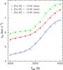 |
Fig. 1 Calibration between the width of the CCF of a non-rotating star, σ0, and its effective temperature. A fourth-order polynomial fit is shown. |
Uncertainties in vsini were estimated by error propagation. We considered a conservative uncertainty of 0.09 km s-1 as the uncertainty in σobs, as derived from the standard deviation of σobs for stars with more than one observation. Regarding the uncertainties in σ0, we considered the rms of the σ0-Teff calibration and the errors in the effective temperature (see below). We should caution that the errors in vsini tend to increase towards lower vsini values. While stars with vsini larger than 2.0 km s-1 show median errors of the order of 0.20 km s-1, this number increases to 0.45 km s-1 for stars with vsini between 1 and 2.0 km s-1, and 0.65 km s-1 for stars with vsini below 1 km s-1. Some stars show large errors making their vsini values compatible with zero. For these stars we provided upper limits (computed as vsini + Δvsini).
We are aware that a more detailed error analysis needs a comprehensive study of the dependence of σobs on the signal-to-noise ratio (S/N) and on the depth of the CCF (see e.g. Melo et al. 2001, and references therein). In particular, our trend of lower uncertainties towards higher vsini may be influenced by the fact that higher vsini values translate into lower CCF depths and, therefore, higher errors on σobs. Since the dependence of σobs on parameters such as the spectra S/N or the CCF depth is also crucial in order to determine the errors when measuring radial velocities (one of the main purposes of the HADES survey), we leave such a study for a forthcoming work. Here we note that our estimated uncertainties are compatible with the uncertainties reported in the literature when using the CCF technique, typically in the range 0.3–0.6 km s-1 (e.g. Browning et al. 2010).
Since we are considering stars with very slow rotation, our capability of measuring the projected rotational velocity is linked to an accurate determination of σ0. It might be the case that for very slow rotators (σobs⋍σ0) our calibration returns a σ0 value slightly larger than σobs. In these cases upper limits were determined as follows. For slow rotators we can write σobs = σ0 + ϵ, where ϵ≪σ0, and therefore Eq. (2) leads to  (3)As we are in the very slow rotation domain, it is reasonable to assume ϵ ~ Δσ0. Two main sources of uncertainty in σ0 were considered: the errors associated with the stellar effective temperature, which are of the order of 70 K, and the errors associated with the σ0-Teff calibration, for which we consider its corresponding rms. The derived vsini values, errors, and upper limits are listed in Table A.1.
4. Spectral subtraction
4.1. Reference inactive stars
In order to determine the emission excess in the different chromospheric indicators we subtract the underlying photospheric contribution from the stellar spectrum. To do this we employed the spectral subtraction technique (e.g. Frasca & Catalano 1994; Montes et al. 1995a, 2000). This technique automatically subtracts the basal chromospheric flux provided that the spectrum of a non-active star of similar stellar parameters and chemical composition to the target star is used as reference (Martínez-Arnáiz et al. 2010).
To select our quiet templates for each star and each observation the Ca ii H & K S index was computed. Our definition of the bandpasses for the S index is made following Henry et al. (1996). The fluxes in the central cores of the Ca ii H & K lines are measured in two windows, 3.28 Å in width and centred at 3968.47and 3933.67 Å, respectively. Continuum fluxes on the sides of the lines are measured in two 20 Å windows with central wavelengths at 3901.07 and 4001.07 Å. Fluxes were measured using the IRAF6 task sbands. Before measuring the fluxes, each individual spectrum was corrected for its corresponding radial velocity using the IRAF task dopcor. No attempt to convert our S index into the Mount Wilson scale or to correct it from the underlying stellar photospheric contribution was done. We note that although Suárez Mascareño et al. (2015) extended the original  calibration by Noyes et al. (1984) up to (B−V) ~ 1.9, the use of is not needed for the purpose of this work.
Figure 2 shows the median S index value as a function of the stellar effective temperature for each star. Given that our sample covers a wide range of S index values, it is reasonable to assume that the stars with the lowest S index (those stars lying on the dashed line in Fig. 2) are the least active stars in our sample. These stars (namely GJ 15A, GJ 184, GJ 412A, GJ 720A, GJ 3997, GJ 4092, and V* BR Psc) were selected as references for the spectral subtraction for all the activity indicators.
The star GJ 4196 also lies among the lowest S index stars in the sample, but it was not selected as reference for the spectral subtraction because it has a metallicity value that is significantly larger than the remaining reference stars (see next section). It is worth noting that metallicity effects are usually not taken into account in the computation of the S index, although Lovis et al. (2011) noticed that for metal-poor stars the continuum passbands are weaker, resulting in slightly larger S values.
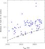 |
Fig. 2 Median S index for each star vs. stellar effective temperature. The dashed line represents a fit to those stars with the lowest S values (shown with circles). The star GJ 4196 (see text) is shown with a diamond symbol. |
4.2. Emission excess fluxes
An extensive description of the procedure adopted to compute the excess fluxes is provided by Scandariato et al. (2017). Here we give a summary of the reduction steps that lead to the measurement of the flux excess.
The spectra provided by the DRS show night-to-night variations in the continuum level at different wavelengths; the variations are due to atmospheric differential absorption and instrumental effects. To correct them, and to scale the observed spectra to the same flux reference, we compared them with synthetic spectra from the BT-Settl spectral library provided by Allard et al. (2011). The library was interpolated in order to obtain a model atmosphere for each star with its corresponding stellar parameters (Teff, log g, and [Fe/H]). Both the observed spectra and the model were degraded to a low-resolution (down to R< 50) in order to avoid discrepancies between the observed and the model lines profiles. Finally, the spectrum-to-model flux ratio was used to rescale the observed high-resolution spectrum. The flux-rescaled spectra were then corrected for telluric contamination using the spectrum of the telluric standard η UMa observed with the same spectrograph used in this work by our group within the context of the GAPS program (see Borsa et al. 2015). For each star, we also computed the median of all the corresponding observed spectra.
For each star in our sample, we interpolated the grid of the median spectra of the selected reference stars (see previous section) over Teff. Before performing the interpolations, the rotational broadening (as measured in this work) of both the observed and reference spectra were applied. The rotational broadening was performed by convolving each stellar spectrum with the required rotational profile, as provided by Gray (2008). Stellar metallicity was also taken into account as our reference stars have relatively low metallicities. This is in part because the continuum flux predicted by the BT-Settl atmosphere models decreases towards lower metallicities. The result is an offset between the observed and template fluxes with the observed fluxes being lower than the references values. In order to correct for this offset, a low-order polynomial fit was applied. Finally, line flux excesses were computed by integrating the difference spectrum in the wavelength ranges listed in Table 1. These ranges were set after a visual inspection of the subtracted spectra. Errors in the flux excesses were estimated by propagating the S/N of the subtracted spectrum out of the core of the lines.
Chromospheric emission lines analysed in this work.
It is worth noting that for some stars showing calcium emission we were not able to measure any Hα emission. This might be related to the complex mechanisms involved in the Hα emission. We considered emission excesses in the subtracted spectrum, and it was shown that at relatively low-activity levels (such as the ones in our sample) the flux radiated in the Hα line seems to initially decrease with increasing calcium flux, resulting in an Hα extra-absorption (Robinson et al. 1990; Walkowicz & Hawley 2009; Scandariato et al. 2017).
5. Other stellar properties
5.1. Spatial velocity components and age
Stellar age is one of the most difficult parameters to obtain accurately. A rough age estimate can be obtained if the star is a member of a stellar kinematic group or a young stellar association. Indeed, it seems that most of the active early-M dwarfs may belong to young associations (Reiners et al. 2012). However, it should be noted that identifying stars in kinematic groups is not a trivial task. Lists of members change among different works and many old stars can share the spatial motion of young stars in kinematic groups. For example, López-Santiago et al. (2009) show that among previous lists of Local Association members, roughly 30% are old field stars. Therefore, kinematic criteria alone are not sufficient to reach a conclusion on the young nature of a star on a robust basis. A combination of kinematics, spectroscopic signatures of youth (e.g. rotation, activity), and the location of the stars in colour-magnitude diagrams are usually used to assess the likelihood of membership of a star to young kinematic groups (e.g. Montes et al. 2001a; Maldonado et al. 2010).
Galactic spatial-velocity components (U,V,W) were computed for our targets using the mean radial velocity measured within the HADES project together with parallaxes and proper motions (Reid et al. 1995; Lépine 2005). To compute (U,V,W) we followed the procedure of Montes et al. (2001b) and Maldonado et al. (2010). It is known that binarity might alter the derived kinematic properties in the case of close-in binaries. It is, however, more unlikely that for wide visual binaries the classification of a system as kinematically old/young might be affected. Furthermore, catalogues of binaries might include many optical (non-physical) systems. Therefore, in the analysis we kept the stars in binary systems listed in the CCDM (Dommanget & Nys 2002), the WVDSC catalogue (Mason et al. 2001), or in Simbad (Wenger et al. 2000). A total of 16 stars (~23% of the sample) have an entry in at least one of these catalogues. In order to identify close-in spectroscopic binaries, the SB9 (Pourbaix et al. 2004) and CAB3 (Eker et al. 2008) catalogues were searched, but no match was found. We note that as the HADES project is an exoplanet survey, those stars for which signatures of a close-in stellar companion have been found were excluded from the survey and not considered for further follow up.
Figure 3 shows the (U,V) and (W,V) planes. We identified as kinematically young those stars inside or near the boundary of the young disc population as defined by Eggen (1984, 1989). A total of 37 stars (roughly 51% of the whole sample) were classified as kinematically young (possible ages ≲650 Myr, i.e. the age of the Hyades open cluster). The fraction of possible young stars among the single stars is 29/55 (i.e. ~53%); among the binaries, 8/16 (50%) of the stars are kinematically young. Our derived (U,V,W) velocities are given in Table A.2.
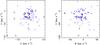 |
Fig. 3 (U,V) and (W,V) planes for the observed stars. The dashed red line represents the boundary of the young disc population as defined by Eggen (1984, 1989). Stars inside or close to this boundary are shown with filled circles. Stars flagged as binaries are shown with diamonds. |
5.2. X-ray fluxes
We searched for X-ray counterparts by collecting the count rates and hardness ratio data provided by the heasarc7 archive determined from the PSPC instrument on board the ROSAT mission (Voges et al. 1999, 2000). To determine the X-ray fluxes we used the count rate-to-energy flux conversion factor (CX) relation given by Schmitt et al. (1995) (4)where HR is the hardness ratio of the star in the ROSAT energy band 0.1–2.4 KeV, defined as HR = (H−S)/(H + S) where H and S refers to counts in the hard (0.5–2.0 KeV) and soft (0.1–0.4 KeV) bands, respectively. Combining the X-ray count rate, fX(counts s-1) and the conversion factor CX with the distance d (pc), the stellar X-ray luminosity LX(erg s-1) can be estimated. This approach assumes that absorption effects are not of significant importance as our targets are near by (d ≲ 45 pc). For two targets (GJ 9440 and GJ 476) X-ray fluxes were taken directly from the XMM XAssist Source List (Ptak & Griffiths 2003).
6. Results
Our stellar sample is presented in Table A.1 where the basic stellar parameters are listed. Kinematic and ancillary data are shown in Table A.2. Finally, our derived emission excesses are listed in Table A.3.
6.1. Relationships between rotation, activity, and stellar parameters
6.1.1. Activity versus effective temperature
Figure 4 shows the excess log (Fλ/FBol) values as a function of the stellar effective temperature, where bolometric fluxes were computed from the stellar luminosities and radii given in Table A.1. Although there is a large scatter, the strength of the emission excess is roughly constant for the stars in the temperature range studied here (3400–3980 K, spectral types K7.5-M3). This result holds for all the considered activity indicators. This is in line with previous works showing that the strength of the activity is constant for early-mid M types (Hawley et al. 1996; West et al. 2004; West & Hawley 2008; Reiners et al. 2012; Stelzer et al. 2013a). The comparison with the literature samples also reveals the low-activity levels of our sample. While most of our stars show values of log (FHα/FBol) lower than –5.0, the values in the literature are typically in the range between –3.0 and –4.5.
We also note that the median log Fλ values are higher in the calcium lines. It also tends to decrease through the Balmer lines towards lower wavelengths, from 4.72 [erg cm-2 s-1] for Hα to 3.78 [erg cm-2 s-1] for Hϵ. This is likely related to the different heights or regions where the lines are formed.
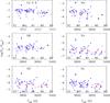 |
Fig. 4 Values of log (Fλ/FBol) vs. the stellar effective temperature (K). Possible young stars according to our kinematic analysis are shown with filled symbols. Median binned values are overplotted as red squares. The relationship between Teff and spectral type is taken from Maldonado et al. (2015). |
6.1.2. Rotational velocity versus effective temperature
We next explore the correlation between rotation and effective temperature. Figure 5 shows the derived vsini values as a function of Teff. Several conclusions can be drawn from this figure. First, we note the very low rotation levels of our sample. Only four stars show vsini values larger than 2.5 km s-1, namely GJ 9793, TYC 1795-941-1, TYC 3720-426-1, and TYC 2703-706-1. Although our sample might be biased towards slow rotating stars, our analysis is in agreement with previous results suggesting that rotation levels larger than about 2.5 km s-1 are rare in old field M stars (e.g. Marcy & Chen 1992; Browning et al. 2010).
Figure 5 also shows that our ability to measure vsini severely diminishes as we move towards cooler stars. In particular, for stars cooler than 3700 K, ~72% of the measurements correspond to upper limits. Furthermore, our estimated uncertainties slightly increase towards cooler stars. We also note that there seems to be a tendency to lower rotation levels as we move towards cooler stars. This is especially evident if we look at the binned vsini values (red squares in Fig. 5). These two effects may be related. We should first note that the errors in vsini tend to increase towards lower vsini values and it could be that errors on vsini increase towards cooler stars just because the vsini diminishes towards lower temperatures. This reflects a relation between low rotation rates and late-type stars, and also reflects the difficulty in deriving accurate vsini values for these stars.
In order to test whether a temperature-rotation correlation is present in our data several statistical tests were performed: i) the Spearman’s correlation test excluding upper limits; and ii) the generalised Kendall’s τ and generalised Spearman’s ρ correlation tests. The last two were performed using the ASURV code (Feigelson et al. 2014), which implements the methods presented in Isobe et al. (1986). Table 2 shows the results. While the Spearman’s test (excluding upper limits) suggests that there is no correlation, the results from the generalised Kendall’s and Spearman’s tests are compatible with a moderate but statistically significant trend of lower rotation levels towards cooler stars. This result, however, should be regarded with caution as it could be the case that the kinematically old stars in our sample are cooler than the possible young ones. While a K-S test shows no significant differences in the Teff distribution of kinematically young/old stars (D ~ 0.15, p ~ 0.77), a slightly lower fraction of kinematically young stars towards cooler temperatures might be present in our data (45.8%, 66.7%, 57.1%, 44.4%, and 33.3%, for stars in the Teff ranges 3800–3900 K, 3700–3800 K, 3600–3700 K, 3500–3400 K, 3500–3600 K, and 3400–3500 K, respectively).
If confirmed, the trend of lower rotation levels towards cooler stars might appear to be in contradiction with Browning et al. (2010) who found that the fraction of stars with vsini larger than 2.5 km s-1 increases towards lower masses. However, we note that these authors consider stars with spectral types from M0 to ~M6, while our sample is limited to M3. In particular, the rise in the fraction of stars with vsini> 2.5 km s-1 noted in Browning et al. (2010) seems to start at spectral types around M3/M3.5, i.e. corresponding to the transition between partially and fully convective stars where the values and the spread on the vsini are known to be large (see e.g. Reiners et al. 2012; Stelzer et al. 2013b). For hotter stars, our results do not seem to differ from Browning et al. (2010, Fig. 2). Furthermore, although the sample of Browning et al. (2010) was selecting for radial velocity monitoring, no selection of low-activity targets was made. Indeed, the authors cautioned that their sample may be biased towards nearby and implicitly young (and somewhat more rapidly rotating) targets. These results are also in line with the findings by Delfosse et al. (1998) who found no measurable rotation for stars in the range M0-M3, while they identified an increasing fraction of rotating stars among their sample of dynamical young stars for spectral types above M3.
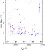 |
Fig. 5 Values of vsini vs. the effective temperature. Upper limits on vsini are shown with arrows. Possible young stars are shown with filled symbols. Typical uncertainties are also shown. Median binned values (without considering upper limits) are overplotted as red squares. |
6.1.3. Rotational velocity – activity relationship
Figure 6 shows the flux excess of the Ca ii k (left) and Hα (right) emission as a function of our measured vsini values. The figure reveals for both lines a mild tendency of higher vsini values with increasing activity strength. We should caution that several factors may be affecting our study.
To start with, we consider vsini values and not rotational periods so the sini term introduces additional scatter, and long rotation periods are not covered8 (e.g. West et al. 2015). Furthermore, our sample is limited to a narrow range of spectral type. Furthermore, our sample is also biased towards low-rotation and low-activity stars. As in the previous section, several statistical tests were performed. Table 2 shows the results for the Ca ii k and Hα line. We conclude that the statistical tests suggest that a moderate but significant correlation between activity and rotation might be present in our data. We also note that both the strength and the statistical significance of the correlation are higher in the Ca ii k than in the Hα line.
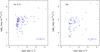 |
Fig. 6 Ca ii K (left) and Hα (right) line emission excess flux vs. vsini. Possible young stars according to our kinematic analysis are shown with filled symbols. Upper limits on vsini are shown with arrows, while the typical error bar is shown in the lower right corner. |
We are aware that the visual inspection of Fig. 6 does not clearly support the results from the statistical tests as the majority of the stars show projected rotational velocities on the 1–2 km s-1 range, most show upper limits on vsini, and the range of rotational velocities considered here is rather small (up to 4 km s-1). In order to check the statistical significance of the possible activity-rotation correlation, all the statistical tests were repeated excluding the stars with the highest rotational velocities (vsini> 2.5 km s-1). In this way we can check whether or not the correlation is dominated by these few stars. The results are given in Table 3. As expected, both the strength and the statistical significance of the correlation clearly diminishes. However, the statistical significance of the correlations (for the analysis including the upper limits) are still well beyond 98% (the typical admitted threshold for considering statistical significance).
We conclude that a hint of a rotation-activity correlation might be present in our data, although the analysis of larger samples of stars covering a wider range of rotation and with measured photometric periods might be needed to clearly confirm this.
Results from Spearman’s correlation test and the generalised Kendall’s τ and Spearman’s ρ correlation tests.
Results from Spearman’s correlation test and the generalised Kendall’s τ and Spearman’s ρ correlation tests, excluding those stars with vsini> 2.5 km s-1.
6.1.4. Age effects
Starting approximately from the zero age main sequence (ZAMS), stellar activity and rotation are expected to decrease with time as a star loses angular momentum with stellar winds via magnetic braking (Weber & Davis 1967; Jianke & Collier Cameron 1993).
A total of 37 stars were classified as kinematically young (see Sec. 5.1), although as cautioned some of them might indeed be old field stars. In order to compare the log Fλ values between possible young and old stars, a series of two-sided Kolmogorov-Smirnov (K-S) tests were performed. The results are given in Table 4, while the cumulative distribution functions of log Fλ for two lines (Ca ii K and Hα) are shown in Fig. 7. The results show a clear tendency for kinematically young stars to show higher levels of activity in the Ca ii H & K lines and in the Balmer lines. We are not able to reject the null hypothesis of both samples coming from the same parent distribution when considering the Balmer line Hγ line, but even for this line we should note the very low p-value returned by the K-S analysis.
Results of the K-S tests performed in this work between possible young disc and old stars.
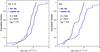 |
Fig. 7 Cumulative distribution function of log Fλ for the Ca ii K (left) and Hα (right) lines. |
6.1.5. X-ray emission versus stellar parameters
We now consider the relationships between rotation and stellar parameters and the X-ray emission. The comparison of the X-ray emission with the optical fluxes is presented in Sect. 6.4. A total of 29 among our stars have available X-ray data. This figure represents ~41% of the total sample. The fraction of stars with X-ray detections is slightly smaller for the stars identified as binaries (~31%) than for stars without known stellar companions (~47%).
The analysis of the X-ray emission as a function of the effective temperature (Fig. 8 left panel) shows a significant scatter with log (FX/FBol) values ranging from –3.3 to –5.1, although most of the stars (~79%) show values between –4.25 and –5.1. These values are lower than the median value of –3.95 found by Stelzer et al. (2013b) in a study of the nearby (within 10 pc) M dwarfs, although this work includes M dwarfs up to spectral type M7. The figure does not reveal a clear trend of the X-ray emission with the effective temperature in line with the results found when considering the optical activity indicators (Sect. 6.1.2).
The middle panel in Fig. 8 shows log FX as a function of the projected rotational velocities vsini. It can be seen that for low (<2 km s-1) vsini values the scatter in the X-ray values is large. The stars with the largest vsini also show the largest X-ray emission. The statistical analysis of the data (see Table 2) shows that the probability that the X-ray fluxes and vsini are correlated by chance is relatively low (~1–2%) with correlation coefficients of the order of 0.40.
We also compared the distribution of X-ray emission for the kinematically old and possible young stars (Fig. 8 right panel). As a whole, there seems to be no difference between possible young and old stars (a K-S tests returns the values D ~ 0.29, p ~ 0.50). However, the figure reveals that while the log FX distribution of kinematically selected young and old stars seems to be identical for values of X-ray emission log FX< 5.5 erg cm-2 s-1, at larger values possible young stars clearly tend to show larger X-ray emission values than old stars.
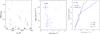 |
Fig. 8 X-ray emission as a function of the stellar parameters. Left panel: log (FX/FBol) vs. stellar effective temperature. Middle panel: X-ray flux, log FX, vs. vsini. Right panel: cumulative distribution function of log FX. Colours and symbols are as in the previous figures. |
6.2. Balmer decrements
Ratios between pairs of fluxes, in particular the Balmer decrements (e.g. Hα/Hβ), are indicators of the physical conditions of the emitting regions (e.g. Landman & Mongillo 1979; Chester 1991).
Figure 9 shows the Balmer decrement FHα/FHβ as a function of the effective temperature. Typical values of solar plages and prominences (see e.g. Landman & Mongillo 1979; Chester 1991) are overplotted for comparison. The figure shows the wide range of FHα/FHβ values covered by our sample. The stars in our sample with Teff> 3800 K show a decreasing trend in FHα/FHβ as we move towards cooler stars. Three of our hottest stars (GJ 9404, GJ 548A, and StKM 1-650) show values of the Balmer decrement compatible with or above the region of solar prominences9. For stars in the spectral range between ~M0 and M1.5, most of the Balmer decrements (FHα/FHβ) show values compatible with those of solar plages.
Our results can be compared with pre-MS M stars (Stelzer et al. 2013a) and the active M dwarf templates from the Sloan Digital Sky Survey (Bochanski et al. 2007) and with the results by Frasca et al. (2015) who analysed the Balmer decrement of magnetically active stars and accretors in two young regions (Chamaeleon I and γ Velorum), with the exception of two strong accreting stars in their sample which have values of FHα/FHβ close to ~30. All these samples are also shown in Fig. 9. It is clear from the figure that the pre-MS sample and the active M dwarf templates both show a trend of increasing FHα/FHβ decrement with decreasing temperature. As this is the opposite of what we found for our K7-M0 dwarfs one might speculate about the possibility of some bias affecting our earliest stars, for example their slightly higher vsini on average (as larger decrements might be expected for faster rotating stars). However, the values of the FHα/FHβ decrements shown by our stars with Teff> 3800 K agree very closely with the decrement values found in the pre-MS sample and in the Frasca et al. (2015) sample (roughly between 2.0 and 5.0, i.e. between solar plages and prominences). For our M dwarfs with Teff< 3800 K, the values of the Balmer decrements are clearly lower than the literature samples (below 2.0) confirming the low-activity levels of our sample.
Finally, we also note that the Balmer decrement shows no difference between possible young and old disc stars, except that there seems to be no kinematically young stars among the “prominence-like” stars.
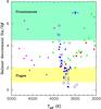 |
Fig. 9 Balmer decrement FHα/FHβ vs. the effective temperature. Possible young stars are shown with filled symbols. Green stars denote pre-MS M stars from Stelzer et al. (2013a), red triangles correspond to the active M dwarf templates from the Sloan Digital Sky Survey (Bochanski et al. 2007), while data from Frasca et al. (2015) is shown in purple squares. Typical ranges of solar plages and prominences are shown as hatched areas. Typical uncertainties are also shown. |
6.3. Flux-flux relationships
Figures 10 and 11 show the comparison between pairs of fluxes of different chromospheric lines for the stars in our sample. Power-law functions were fitted to the data, 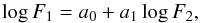 (5)where F1 and F2 are the fluxes of two different lines and a0 and a1 the fit coefficients. We note here that we are considering the flux excesses measured over the combined spectra, so for each star all the fluxes are obtained from the same average spectrum. Several samples are overplotted for comparison: a sample of F, G, and K stars from López-Santiago et al. (2010), Martínez-Arnáiz et al. (2010, 2011); a sample of late-K and M dwarfs (from the same authors); and a sample of pre-MS M stars from Stelzer et al. (2013a). For better comparison with our data, from the last sample only stars in the spectral range K7-M3 were considered. The values of a0 and a1 are given in Table 5. The fits were performed with the least-squares bisector regression described by Isobe et al. (1990). Stars with large errors in the fluxes were excluded from the fits.
Our sample of M dwarfs seems to follow the same trend as FGK stars and other late-K/early-M dwarfs in the Ca ii H vs. Ca ii K plane (Figure 10, left panel) without any obvious deviation between both samples. The Hα vs. Ca ii K plot is shown in the right panel of Fig. 10. Martínez-Arnáiz et al. (2011) identified two branches in the flux-flux relationships when one of the considered activity diagnostics is the Hα line. The inactive branch is composed of the majority of the stars and occupied by field stars with spectral types from F to M. The deviating stars, on the other hand, constitute the upper or active branch, which is composed of young late-K and M dwarfs with saturated Hα emission. In Fig. 10, right panel, it can be seen that our M dwarfs are located in the region of the plot corresponding to the inactive branch. However, our derived slope is steeper (~2) than the previously reported values (~1). In addition, a vertical offset seems to be present in our sample in comparison with the literature sample. It seems that on the whole, our sample of M dwarfs is located slightly above the inactive branch, or in other words, there seems to be a lack of stars with low Hα emission.
We also note that two of our targets (TYC3720-426-1 and TYC2703-706-1) seem to follow the same tendency of the stars in the active branch. These two stars were not considered in the fits and are discussed in more detail in the next subsections.
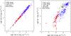 |
Fig. 10 Flux-flux relationships between calcium lines (Ca ii H & K, left panel), and between Hα and Ca ii K (right panel). M dwarfs from this work are plotted with red filled squares; FGK stars from López-Santiago et al. (2010), Martínez-Arnáiz et al. (2010, 2011) with open circles, late-K and M stars from the literature (same references as for FGK stars) are shown by purple open squares; green stars denote the M0-M3 pre-MS M stars from Stelzer et al. (2013a). Possible young disc stars in our M star sample are shown by circles. The two stars discussed in Sect. 6.5 are indicated by diamonds. The black dash-dotted line represents our best fit; the relations for the “active” and “inactive” branches by Martínez-Arnáiz et al. (2011) are shown in light grey solid and dashed dark grey lines, respectively. |
Coefficients of the flux-flux relationships.
Regarding the slopes between the different Balmer lines, Fig. 11 shows that our sample of M dwarfs follows a similar tendency to the solar-type stars from the literature. The sample of pre-MS dwarfs also behave in the same way as the rest of stars. Our derived slopes for the flux-flux relationships have values ~1.0/1.2 and are compatible with previously reported values (even though these literature values correspond to studies of pre-MS stars and/or include “ultra-cool” dwarfs; see references in Table 5). The Hϵ line shows a slightly lower slope than 1.0 (~0.80), in agreement with previous works (Montes et al. 1995b, 1996a), although for ultra-cool dwarfs (including stars up to spectral type M9) Stelzer et al. (2012) reports a slope close to 3.0.
We should caution that there are few literature stars to use for comparison as the Balmer fluxes for a large fraction of the literature stars are not reported. Furthermore, nearly all the stars in the comparison samples with available fluxes in the Balmer lines are stars of the active branch. This explains the apparent lack of comparison stars at low fluxes in Fig. 11 (in contrast to the log F(Hα) vs. log F(Ca ii K) plot where our M stars are mixed with the literature M dwarf sample, see Fig. 10).
We conclude that our sample of M dwarfs is complementary to the literature samples in the sense that they follow similar flux-flux relationships. Our sample constitutes an extension of the analysis of the Ca ii H & K and Balmer flux-flux relationships of main-sequence M dwarfs to the very low flux domain.
6.4. Chromospheric-corona flux-flux relationships
In addition to the flux-flux relationships between different chromospheric activity indicators, the chromospheric-coronal relation was also studied. All stars with X-ray detections show Ca ii K emission with only one exception (GJ 412A); regarding Hα, only 69% of the stars with X-ray data show emission in this line. Figure 12 shows the X-ray flux, log FX, as a function of the fluxes in the Ca ii K line (left) and Hα (right).
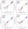 |
Fig. 11 Flux-flux relationships between Balmer lines: Hα, Hβ, (top left panel); Hα, Hγ (top right panel); Hα, Hδ (bottom left); and Hα, Hϵ (bottom right). Colours and symbols are as in Fig. 10. |
No distinction between active and inactive branches was found in the literature for the log FX vs. Ca ii K line and Hα flux-flux relationships (Martínez-Arnáiz et al. 2011)10. Our sample of M dwarfs seems to follow the same tendency as the literature estimates. Our analysis, however, clearly reveals that our M dwarfs have lower levels of X-ray fluxes than the FGK stars. Figure 12 also shows those of our M dwarfs with larger deviations from the literature samples are the ones with lowest X-ray and chromospheric emission.
Our lower levels of X-ray fluxes translates into significant lower slopes than the ones previously reported in the literature (see Table 5). As before, it is important to note that some previous works are based on pre-MS stars or include cooler stars than ours. Also, the analysis presented in Montes et al. (1995b, 1996a) is based on binary stars in chromospherically active systems, which might explain their significantly higher (>2.0) slopes.
The two stars discussed in Sect. 6.5 are in the same place or close to the place occupied by the pre-MS M stars in Fig. 12. Furthermore, they show levels of X-ray activity compatible with or close to saturation (LX/LBol ~ 10-3) and were identified in the active branch in the Hα vs. Ca ii K plot. This agrees with previous works suggesting that the stars in the active branch are young or flare stars with saturated X-ray emission (e.g. Martínez-Arnáiz et al. 2011).
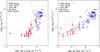 |
Fig. 12 Flux-flux relationships between X-ray and the calcium line Ca ii K (left panel), and between X-ray and the Hα line (right panel). Colours and symbols are as in Fig. 10. |
6.5. Notes on interesting stars
Here we give further details on the two stars, whose position in the flux-flux diagrams is consistent with the position of the 1−10 Myr old pre-MS stars from the literature.
TYC3720-426-1
This M0 star has the largest vsini (4.07 km s-1) and strongest X-ray emission (log (LX/LBol) = –3.29) in our sample. It shows emission in all the Balmer lines and in the Na i D1, D2 doublet. It is the second star in our sample with the largest median S index. Its kinematics are compatible with being a member of the Local Association of stars, in particular Zuckerman et al. (2011), Malo et al. (2013) classified it as a member of the Columba nearby young association (~30 Myr). Using the BANYAN II online tool (Malo et al. 2013; Gagné et al. 2014), which implements a Bayesian analysis to determine probabilities of membership to nearby young kinematic groups together with the HADES radial velocities, we found a 61% membership probability for this star to be a member of the Columbia association. From the SuperWASP archive11 photometry a rotation period of 4.65 ± 0.03 days can be inferred. The position of this star in a period-colour diagram agrees reasonably well with the age of the Columba association.
TYC2703-706-1
TYC2703-706-1 is an M0.5 dwarf which has the largest activity S index in our sample. All its activity indicators (including the Na i D1, D2 doublet and the He i D3 line) appear in emission. It also has one of the highest rotation levels (vsini of 3.32 km s-1) and a large fractional X-ray luminosity (log (LX/LBol) of –3.48). Its galactic spatial velocity components suggest that it is a young disc star. Indeed, it has been identified as a candidate member12 of the young (~23 Myr) β Pic stellar association (Schlieder et al. 2012). However, our analysis with the BANYAN II tool reports a probability of 0% of its being a member of this association. The analysis of the SuperWASP photometry reveals a rotation period of 8.00 ± 0.05 days. This period falls in the upper boundary of the period distribution of the bona fide β Pic members, suggesting an age equal to or slightly younger than the β Pic members.
7. Discussion and conclusions
In spite of the increasing effort devoted to the study of M dwarfs, our understanding of their chromospheres and the processes that we generally call “activity” are still very far from being fully understood. In this work, a detailed analysis of the relationships between activity and stellar parameters (rotational velocity, effective temperature, age) and the flux-flux relationships in a large sample of early M-dwarfs is presented. Projected rotational velocities vsini are computed using the CCF technique, while emission excess fluxes in the Ca ii H & K and Balmer lines are derived using the spectral subtraction technique.
In spite of the presence of some potential biases due to the fact that our sample was selected for a radial velocity search program (i.e. selected with low levels of activity), our study reveals several interesting trends. First, the strength of the chromospheric line emission seems to be constant in the spectral range studied here (M0-M3). This holds for all the activity indicators considered. Second, field early-M dwarfs have very low vsini values with a tendency of lower rotation levels as we move towards cooler stars up to spectral type M3, although this might need confirmation as the fraction of possible young stars seems to decrease towards cooler stars (there could also be a possible inversion for later spectral types as discussed in Sect. 6.1.2). Third, the analysis suggests that a moderate but statistically significant correlation between activity and rotation might be present in our data. Finally, possible young stars show higher levels of emission excess in the Ca ii H & K lines and most of the Balmer lines than probable old disc stars. These findings agree reasonably well with previous works, suggesting that the already established activity-rotation-age relationship found in FGK stars also holds for early M-dwarfs.
The comparison between pairs of fluxes of different chromospheric lines has revealed other interesting trends. The analysis of the Balmer FHα/FHβ decrement shows a trend of decreasing values, from values compatible with solar prominences for stars with Teff ~ 3900 K to values similar to those of the solar plages for Teff ~ 3750 K. Then, the Balmer decrement remains roughly constant in the range 3750–3600 K.
On the other hand, the analysis of the flux-flux relationships shows that our M dwarfs sample is complementary to other literature samples, extending the analysis of the flux-flux relationships to the low-chromospheric fluxes domain. Our results confirm that field stars deviating from the “general” flux-flux relationships are likely to be young. The low values of the chromospheric excess of our M stars is also revealed in the corona-chromosphere flux-flux relationships. We conclude that our sample represents a benchmark for the characterisation of magnetic activity at low levels.
Understanding the chromospheres of M-dwarfs is crucial for ongoing exoplanet searches. While early surveys tried to avoid active M dwarfs, there is ongoing evidence that M dwarfs show radial velocity signals due to the simultaneous presence of low-mass planets and activity-related phenomena (e.g. Affer et al. 2016). Furthermore, thanks to new instrumentation at IR wavelengths where lines are less affected by magnetic activity than in the optical (e.g. Amado et al. 2013; Carleo et al. 2016), new surveys are focusing on late-M and young stars. It is therefore essential to understand the mechanisms involved in chromospheric and coronal heating as well as their dependence on the stellar parameters before a full understanding of their effects on exoplanet detection can be reached.
IRAF is distributed by the National Optical Astronomy Observatories, which are operated by the Association of Universities for Research in Astronomy, Inc., under cooperative agreement with the National Science Foundation.
For a typical radius of 0.5 R⊙ and assuming a low vsini of 0.8 km s-1, rotation periods longer than ~32 days are excluded from the analysis.
The stars BPM 96441 and 2MASS J22353504+3712131 were excluded from the analysis because their large errors in FHβ make the derived decrements unreliable.
The authors do find, however, the two branches in the X-ray vs. Ca ii IRT, 8498 Å line analysis. Unfortunately, the Ca ii IRT lines are not covered by our spectra.
Flagged with a value of 2 on a scale from 1 to 4, where 4 means the best candidates.
Acknowledgments
This work was supported by the Italian Ministry of Education, University, and Research through the PREMIALE WOW 2013 research project under grant Ricerca di pianeti intorno a stelle di piccola massa. GAPS acknowledges support from INAF through the Progetti Premiali funding scheme of the Italian Ministry of Education, University, and Research. I.R. and M.P. acknowledge support from the Spanish Ministry of Economy and Competitiveness (MINECO) through grant ESP2014-57495-C2-2-R. J.I.G.H. acknowledges financial support from the Spanish Ministry of Economy and Competitiveness (MINECO) under the 2013 Ramón y Cajal program MINECO RYC-2013-14875. A.S.M., J.I.G.H., and R.R. also acknowledge financial support from the Spanish ministry project MINECO AYA2014-56359-P. G.M., L.A., E.M., G.P., and A.S. acknowledge support from the Etaearth project. G.S. and I.P. acknowledge financial support from “Accordo ASI–INAF” No. 2013-016-R.0 July 9, 2013. A. Bayo and B. Montesinos are acknowledged for useful discussions about the BT-Settl models and interpolation.
References
- Affer, L., Micela, G., Damasso, M., et al. 2016, A&A, 593, A117 (Paper I) [NASA ADS] [CrossRef] [EDP Sciences] [Google Scholar]
- Allard, F., Homeier, D., & Freytag, B. 2011, in 16th Cambridge Workshop on Cool Stars, Stellar Systems, and the Sun, eds. C. Johns-Krull, M. K. Browning, & A. A. West, ASP Conf. Ser., 448, 91 [Google Scholar]
- Amado, P. J., Quirrenbach, A., Caballero, J. A., et al. 2013, in Highlights of Spanish Astrophysics VII, eds. J. C. Guirado, L. M. Lara, V. Quilis, & J. Gorgas, 842 [Google Scholar]
- Barnes, S. A. 2007, ApJ, 669, 1167 [NASA ADS] [CrossRef] [Google Scholar]
- Bochanski, J. J., West, A. A., Hawley, S. L., & Covey, K. R. 2007, AJ, 133, 531 [NASA ADS] [CrossRef] [Google Scholar]
- Borsa, F., Scandariato, G., Rainer, M., et al. 2015, A&A, 578, A64 [NASA ADS] [CrossRef] [EDP Sciences] [Google Scholar]
- Browning, M. K., Basri, G., Marcy, G. W., West, A. A., & Zhang, J. 2010, AJ, 139, 504 [NASA ADS] [CrossRef] [Google Scholar]
- Busà, I., Aznar Cuadrado, R., Terranegra, L., Andretta, V., & Gomez, M. T. 2007, A&A, 466, 1089 [NASA ADS] [CrossRef] [EDP Sciences] [Google Scholar]
- Carleo, I., Sanna, N., Gratton, R., et al. 2016, Exp. Astron., 42, 99 [NASA ADS] [CrossRef] [Google Scholar]
- Chester, M. M. 1991, Ph.D. Thesis, Pennsylvania State University, University Park [Google Scholar]
- Cincunegui, C., Díaz, R. F., & Mauas, P. J. D. 2007, A&A, 469, 309 [NASA ADS] [CrossRef] [EDP Sciences] [Google Scholar]
- Claret, A., & Bloemen, S. 2011, A&A, 529, A75 [NASA ADS] [CrossRef] [EDP Sciences] [Google Scholar]
- Cosentino, R., Lovis, C., Pepe, F., et al. 2012, in SPIE Conf. Ser., 8446, 1 [Google Scholar]
- Covino, E., Esposito, M., Barbieri, M., et al. 2013, A&A, 554, A28 [NASA ADS] [CrossRef] [EDP Sciences] [Google Scholar]
- Delfosse, X., Forveille, T., Perrier, C., & Mayor, M. 1998, A&A, 331, 581 [NASA ADS] [Google Scholar]
- Dommanget, J., & Nys, O. 2002, VizieR Online Data Catalog: I/274 [Google Scholar]
- Dressing, C. D., & Charbonneau, D. 2013, ApJ, 767, 95 [NASA ADS] [CrossRef] [Google Scholar]
- Dumusque, X., Pepe, F., Lovis, C., et al. 2012, Nature, 491, 207 [NASA ADS] [CrossRef] [PubMed] [Google Scholar]
- Eggen, O. J. 1984, AJ, 89, 1358 [NASA ADS] [CrossRef] [Google Scholar]
- Eggen, O. J. 1989, PASP, 101, 366 [NASA ADS] [CrossRef] [Google Scholar]
- Eker, Z., Ak, N. F., Bilir, S., et al. 2008, MNRAS, 389, 1722 [NASA ADS] [CrossRef] [Google Scholar]
- ESA 1997, The HIPPARCOS and TYCHO catalogues. Astrometric and photometric star catalogues derived from the ESA HIPPARCOS Space Astrometry Mission, ESA SP, 1200 [Google Scholar]
- Feigelson, E. D., Nelson, P. I., Isobe, T., & LaValley, M. 2014, Astrophysics Source Code Library [record ascl:1406.001] [Google Scholar]
- Finch, C. T., & Zacharias, N. 2016, VizieR Online Data Catalog: I/333 [Google Scholar]
- Fischer, D. A., Howard, A. W., Laughlin, G. P., et al. 2014, Protostars and Planets VI, 715 [Google Scholar]
- France, K., Froning, C. S., Linsky, J. L., et al. 2013, ApJ, 763, 149 [NASA ADS] [CrossRef] [Google Scholar]
- Frasca, A., & Catalano, S. 1994, A&A, 284, 883 [NASA ADS] [Google Scholar]
- Frasca, A., Biazzo, K., Lanzafame, A. C., et al. 2015, A&A, 575, A4 [NASA ADS] [CrossRef] [EDP Sciences] [Google Scholar]
- Gagné, J., Lafrenière, D., Doyon, R., Malo, L., & Artigau, É. 2014, ApJ, 783, 121 [NASA ADS] [CrossRef] [Google Scholar]
- Gray, D. F. 2008, The Observation and Analysis of Stellar Photospheres, ed. D. F. Gray (Cambridge, UK: Cambridge University Press) [Google Scholar]
- Hawley, S. L., Gizis, J. E., & Reid, I. N. 1996, AJ, 112, 2799 [NASA ADS] [CrossRef] [Google Scholar]
- Hawley, S. L., Gizis, J. E., & Reid, N. I. 1997, AJ, 113, 1458 [NASA ADS] [CrossRef] [Google Scholar]
- Henry, T. J., & McCarthy, Jr., D. W. 1993, AJ, 106, 773 [NASA ADS] [CrossRef] [Google Scholar]
- Henry, T. J., Soderblom, D. R., Donahue, R. A., & Baliunas, S. L. 1996, AJ, 111, 439 [NASA ADS] [CrossRef] [Google Scholar]
- Henry, T. J., Jao, W.-C., Subasavage, J. P., et al. 2006, AJ, 132, 2360 [NASA ADS] [CrossRef] [Google Scholar]
- Herrero, E., Ribas, I., Jordi, C., et al. 2016, A&A, 586, A131 [NASA ADS] [CrossRef] [EDP Sciences] [Google Scholar]
- Houdebine, E. R. 2010, MNRAS, 407, 1657 [NASA ADS] [CrossRef] [Google Scholar]
- Howard, A. W., Marcy, G. W., Fischer, D. A., et al. 2014, ApJ, 794, 51 [Google Scholar]
- Isobe, T., Feigelson, E. D., & Nelson, P. I. 1986, ApJ, 306, 490 [NASA ADS] [CrossRef] [Google Scholar]
- Isobe, T., Feigelson, E. D., Akritas, M. G., & Babu, G. J. 1990, ApJ, 364, 104 [NASA ADS] [CrossRef] [EDP Sciences] [Google Scholar]
- Jianke, L., & Collier Cameron, A. 1993, MNRAS, 261, 766 [NASA ADS] [CrossRef] [Google Scholar]
- Kawaler, S. D. 1989, ApJ, 343, L65 [NASA ADS] [CrossRef] [Google Scholar]
- Kiraga, M., & Stepien, K. 2007, Acta Astron., 57, 149 [NASA ADS] [Google Scholar]
- Kraft, R. P. 1967, ApJ, 150, 551 [NASA ADS] [CrossRef] [Google Scholar]
- Landman, D. A., & Mongillo, M. 1979, ApJ, 230, 581 [NASA ADS] [CrossRef] [Google Scholar]
- Leggett, S. K., Allard, F., Berriman, G., Dahn, C. C., & Hauschildt, P. H. 1996, ApJS, 104, 117 [NASA ADS] [CrossRef] [EDP Sciences] [Google Scholar]
- Lépine, S. 2005, AJ, 130, 1680 [NASA ADS] [CrossRef] [Google Scholar]
- Lépine, S., & Gaidos, E. 2011, AJ, 142, 138 [NASA ADS] [CrossRef] [Google Scholar]
- Lépine, S., Hilton, E. J., Mann, A. W., et al. 2013, AJ, 145, 102 [NASA ADS] [CrossRef] [Google Scholar]
- Leto, G., Pagano, I., Buemi, C. S., & Rodono, M. 1997, A&A, 327, 1114 [NASA ADS] [Google Scholar]
- López-Santiago, J., Montes, D., Fernández-Figueroa, M. J., Gálvez, M. C., & Crespo-Chacón, I. 2005, in 13th Cambridge Workshop on Cool Stars, Stellar Systems and the Sun, eds. F. Favata, G. A. J. Hussain, & B. Battrick, ESA SP, 560, 775 [Google Scholar]
- López-Santiago, J., Micela, G., & Montes, D. 2009, A&A, 499, 129 [NASA ADS] [CrossRef] [EDP Sciences] [Google Scholar]
- López-Santiago, J., Montes, D., Gálvez-Ortiz, M. C., et al. 2010, A&A, 514, A97 [NASA ADS] [CrossRef] [EDP Sciences] [Google Scholar]
- Lovis, C., & Pepe, F. 2007, A&A, 468, 1115 [NASA ADS] [CrossRef] [EDP Sciences] [Google Scholar]
- Lovis, C., Dumusque, X., Santos, N. C., et al. 2011, A&A, submitted [arXiv:1107.5325] [Google Scholar]
- Maldonado, J., Martínez-Arnáiz, R. M., Eiroa, C., Montes, D., & Montesinos, B. 2010, A&A, 521, A12 [NASA ADS] [CrossRef] [EDP Sciences] [Google Scholar]
- Maldonado, J., Affer, L., Micela, G., et al. 2015, A&A, 577, A132 [NASA ADS] [CrossRef] [EDP Sciences] [Google Scholar]
- Malo, L., Doyon, R., Lafrenière, D., et al. 2013, ApJ, 762, 88 [NASA ADS] [CrossRef] [Google Scholar]
- Mamajek, E. E., & Hillenbrand, L. A. 2008, ApJ, 687, 1264 [NASA ADS] [CrossRef] [Google Scholar]
- Marcy, G. W., & Chen, G. H. 1992, ApJ, 390, 550 [NASA ADS] [CrossRef] [Google Scholar]
- Martínez-Arnáiz, R., Maldonado, J., Montes, D., Eiroa, C., & Montesinos, B. 2010, A&A, 520, A79 [NASA ADS] [CrossRef] [EDP Sciences] [Google Scholar]
- Martínez-Arnáiz, R., López-Santiago, J., Crespo-Chacón, I., & Montes, D. 2011, MNRAS, 414, 2629 [NASA ADS] [CrossRef] [Google Scholar]
- Mason, B. D., Wycoff, G. L., Hartkopf, W. I., Douglass, G. G., & Worley, C. E. 2001, AJ, 122, 3466 [Google Scholar]
- Melo, C. H. F., Pasquini, L., & De Medeiros, J. R. 2001, A&A, 375, 851 [NASA ADS] [CrossRef] [EDP Sciences] [Google Scholar]
- Messina, S., Pizzolato, N., Guinan, E. F., & Rodonò, M. 2003, A&A, 410, 671 [NASA ADS] [CrossRef] [EDP Sciences] [Google Scholar]
- Messina, S., Monard, B., Biazzo, K., Melo, C. H. F., & Frasca, A. 2014, A&A, 570, A19 [NASA ADS] [CrossRef] [EDP Sciences] [Google Scholar]
- Mohanty, S., & Basri, G. 2003, ApJ, 583, 451 [NASA ADS] [CrossRef] [Google Scholar]
- Montes, D., de Castro, E., Fernandez-Figueroa, M. J., & Cornide, M. 1995a, A&AS, 114, 287 [NASA ADS] [Google Scholar]
- Montes, D., Fernandez-Figueroa, M. J., de Castro, E., & Cornide, M. 1995b, A&A, 294, 165 [NASA ADS] [Google Scholar]
- Montes, D., Fernandez-Figueroa, M. J., Cornide, M., & de Castro, E. 1996a, in Cool Stars, Stellar Systems, and the Sun, eds. R. Pallavicini, & A. K. Dupree, ASP Conf. Ser., 109, 657 [Google Scholar]
- Montes, D., Fernandez-Figueroa, M. J., Cornide, M., & de Castro, E. 1996b, A&A, 312, 221 [NASA ADS] [Google Scholar]
- Montes, D., Fernández-Figueroa, M. J., De Castro, E., et al. 2000, A&AS, 146, 103 [NASA ADS] [CrossRef] [EDP Sciences] [Google Scholar]
- Montes, D., López-Santiago, J., Fernández-Figueroa, M. J., & Gálvez, M. C. 2001a, A&A, 379, 976 [NASA ADS] [CrossRef] [EDP Sciences] [Google Scholar]
- Montes, D., López-Santiago, J., Gálvez, M. C., et al. 2001b, MNRAS, 328, 45 [NASA ADS] [CrossRef] [MathSciNet] [Google Scholar]
- Montesinos, B., Thomas, J. H., Ventura, P., & Mazzitelli, I. 2001, MNRAS, 326, 877 [NASA ADS] [CrossRef] [Google Scholar]
- Neves, V., Bonfils, X., Santos, N. C., et al. 2012, A&A, 538, A25 [NASA ADS] [CrossRef] [EDP Sciences] [Google Scholar]
- Noyes, R. W., Hartmann, L. W., Baliunas, S. L., Duncan, D. K., & Vaughan, A. H. 1984, ApJ, 279, 763 [NASA ADS] [CrossRef] [Google Scholar]
- Oranje, B. J. 1986, A&A, 154, 185 [NASA ADS] [Google Scholar]
- Osten, R. A., Hawley, S. L., Allred, J. C., Johns-Krull, C. M., & Roark, C. 2005, ApJ, 621, 398 [NASA ADS] [CrossRef] [Google Scholar]
- Perger, M., García-Piquer, A., Ribas, I., et al. 2017, A&A, 598, A26 (Paper II) [NASA ADS] [CrossRef] [EDP Sciences] [Google Scholar]
- Pizzolato, N., Maggio, A., Micela, G., Sciortino, S., & Ventura, P. 2003, A&A, 397, 147 [NASA ADS] [CrossRef] [EDP Sciences] [Google Scholar]
- Pourbaix, D., Tokovinin, A. A., Batten, A. H., et al. 2004, A&A, 424, 727 [NASA ADS] [CrossRef] [EDP Sciences] [Google Scholar]
- Ptak, A., & Griffiths, R. 2003, in Astronomical Data Analysis Software and Systems XII, eds. H. E. Payne, R. I. Jedrzejewski, & R. N. Hook, ASP Conf. Ser., 295, 465 [Google Scholar]
- Queloz, D., Allain, S., Mermilliod, J.-C., Bouvier, J., & Mayor, M. 1998, A&A, 335, 183 [NASA ADS] [Google Scholar]
- Reid, I. N., Hawley, S. L., & Gizis, J. E. 1995, AJ, 110, 1838 [NASA ADS] [CrossRef] [Google Scholar]
- Reiners, A., Joshi, N., & Goldman, B. 2012, AJ, 143, 93 [NASA ADS] [CrossRef] [Google Scholar]
- Robinson, R. D., Cram, L. E., & Giampapa, M. S. 1990, ApJS, 74, 891 [NASA ADS] [CrossRef] [Google Scholar]
- Rutten, R. G. M., Zwaan, C., Schrijver, C. J., Duncan, D. K., & Mewe, R. 1989, A&A, 219, 239 [NASA ADS] [Google Scholar]
- Scandariato, G., Maldonado, J., Affer, J. M. L., Biazzo, K., et al. 2017, A&A, 598, A28 (Paper IV) [NASA ADS] [CrossRef] [EDP Sciences] [Google Scholar]
- Schlieder, J. E., Lépine, S., & Simon, M. 2012, AJ, 143, 80 [NASA ADS] [CrossRef] [Google Scholar]
- Schmitt, J. H. M. M., Fleming, T. A., & Giampapa, M. S. 1995, ApJ, 450, 392 [NASA ADS] [CrossRef] [Google Scholar]
- Schrijver, C. J. 1987, A&A, 172, 111 [NASA ADS] [Google Scholar]
- Schrijver, C. J., & Rutten, R. G. M. 1987, A&A, 177, 143 [NASA ADS] [Google Scholar]
- Schrijver, C. J., & Zwaan, C. 2000, Solar and Stellar Magnetic Activity, Camb. Astrophys. Ser., 34 [Google Scholar]
- Skumanich, A. 1972, ApJ, 171, 565 [NASA ADS] [CrossRef] [Google Scholar]
- Soderblom, D. R., Duncan, D. K., & Johnson, D. R. H. 1991, ApJ, 375, 722 [NASA ADS] [CrossRef] [Google Scholar]
- Sozzetti, A., Bernagozzi, A., Bertolini, E., et al. 2013, in EPJ Web Conf., 47, 3006 [Google Scholar]
- Stelzer, B., Alcalá, J., Biazzo, K., et al. 2012, A&A, 537, A94 [NASA ADS] [CrossRef] [EDP Sciences] [Google Scholar]
- Stelzer, B., Frasca, A., Alcalá, J. M., et al. 2013a, A&A, 558, A141 [NASA ADS] [CrossRef] [EDP Sciences] [Google Scholar]
- Stelzer, B., Marino, A., Micela, G., López-Santiago, J., & Liefke, C. 2013b, MNRAS, 431, 2063 [NASA ADS] [CrossRef] [MathSciNet] [Google Scholar]
- Strassmeier, K. G., Fekel, F. C., Bopp, B. W., Dempsey, R. C., & Henry, G. W. 1990, ApJS, 72, 191 [NASA ADS] [CrossRef] [Google Scholar]
- Suárez Mascareño, A., Rebolo, R., González Hernández, J. I., & Esposito, M. 2015, MNRAS, 452, 2745 [NASA ADS] [CrossRef] [Google Scholar]
- Thatcher, J. D., & Robinson, R. D. 1993, MNRAS, 262, 1 [NASA ADS] [Google Scholar]
- van Leeuwen, F. 2007, A&A, 474, 653 [NASA ADS] [CrossRef] [EDP Sciences] [Google Scholar]
- Voges, W., Aschenbach, B., Boller, T., et al. 1999, A&A, 349, 389 [NASA ADS] [Google Scholar]
- Voges, W., Aschenbach, B., Boller, T., et al. 2000, IAU Circ., 7432, 1 [NASA ADS] [Google Scholar]
- Walkowicz, L. M., & Hawley, S. L. 2009, AJ, 137, 3297 [NASA ADS] [CrossRef] [Google Scholar]
- Walkowicz, L. M., Johns-Krull, C. M., & Hawley, S. L. 2008, ApJ, 677, 593 [NASA ADS] [CrossRef] [Google Scholar]
- Weber, E. J., & Davis, Jr., L. 1967, ApJ, 148, 217 [NASA ADS] [CrossRef] [Google Scholar]
- Wenger, M., Ochsenbein, F., Egret, D., et al. 2000, A&AS, 143, 9 [NASA ADS] [CrossRef] [EDP Sciences] [Google Scholar]
- West, A. A., & Hawley, S. L. 2008, PASP, 120, 1161 [NASA ADS] [CrossRef] [Google Scholar]
- West, A. A., Hawley, S. L., Walkowicz, L. M., et al. 2004, AJ, 128, 426 [NASA ADS] [CrossRef] [Google Scholar]
- West, A. A., Weisenburger, K. L., Irwin, J., et al. 2015, ApJ, 812, 3 [NASA ADS] [CrossRef] [Google Scholar]
- Zuckerman, B., Rhee, J. H., Song, I., & Bessell, M. S. 2011, ApJ, 732, 61 [NASA ADS] [CrossRef] [Google Scholar]
Appendix A: Additional tables
Table A.1 lists all the stars analysed in this work. The table provides star identifier (Col. 1), effective temperature in kelvin (Col. 2), spectral type (Col. 3), stellar metallicity in dex (Col. 4), stellar mass in solar units (Col. 5), stellar radius in solar units (Col. 6), logarithm of the surface gravity, log g, in cms-2 (Col. 7), stellar luminosity, log (L⋆/L⊙) (Col. 8), and projected rotational velocities, vsini in km s-1 (Col. 9). Each measured quantity is accompanied by its corresponding uncertainty.
Table A.2 gives the position and kinematic data: star identifier (Col. 1), right ascension and declination (ICRSJ2000)
(Cols. 2 and 3), proper motions in right ascension and declination in arcsec yr-1 (Cols. 4 and 5), stellar parallax with its uncertainty and reference (arcsec, Cols. 6), radial velocity in km s-1 (Col. 7), galactic spatial-velocity components (U,V,W) in km s-1 (Cols. 8–10), and notes on binarity and possible membership to the young disc population.
Table A.3 provides the derived line emission excess fluxes, log Fλ [erg cm-2 s-1], in the different chromospheric indicators studied in this work and in X-ray.
Basic stellar parameters of the stellar sample.
Kinematic data for the observed stars.
Emission excesses, log Fλ [erg cm-2 s-1].
All Tables
Results from Spearman’s correlation test and the generalised Kendall’s τ and Spearman’s ρ correlation tests.
Results from Spearman’s correlation test and the generalised Kendall’s τ and Spearman’s ρ correlation tests, excluding those stars with vsini> 2.5 km s-1.
Results of the K-S tests performed in this work between possible young disc and old stars.
All Figures
|
Fig. 1 Calibration between the width of the CCF of a non-rotating star, σ0, and its effective temperature. A fourth-order polynomial fit is shown. |
| In the text | |
|
Fig. 2 Median S index for each star vs. stellar effective temperature. The dashed line represents a fit to those stars with the lowest S values (shown with circles). The star GJ 4196 (see text) is shown with a diamond symbol. |
| In the text | |
|
Fig. 3 (U,V) and (W,V) planes for the observed stars. The dashed red line represents the boundary of the young disc population as defined by Eggen (1984, 1989). Stars inside or close to this boundary are shown with filled circles. Stars flagged as binaries are shown with diamonds. |
| In the text | |
|
Fig. 4 Values of log (Fλ/FBol) vs. the stellar effective temperature (K). Possible young stars according to our kinematic analysis are shown with filled symbols. Median binned values are overplotted as red squares. The relationship between Teff and spectral type is taken from Maldonado et al. (2015). |
| In the text | |
|
Fig. 5 Values of vsini vs. the effective temperature. Upper limits on vsini are shown with arrows. Possible young stars are shown with filled symbols. Typical uncertainties are also shown. Median binned values (without considering upper limits) are overplotted as red squares. |
| In the text | |
|
Fig. 6 Ca ii K (left) and Hα (right) line emission excess flux vs. vsini. Possible young stars according to our kinematic analysis are shown with filled symbols. Upper limits on vsini are shown with arrows, while the typical error bar is shown in the lower right corner. |
| In the text | |
|
Fig. 7 Cumulative distribution function of log Fλ for the Ca ii K (left) and Hα (right) lines. |
| In the text | |
|
Fig. 8 X-ray emission as a function of the stellar parameters. Left panel: log (FX/FBol) vs. stellar effective temperature. Middle panel: X-ray flux, log FX, vs. vsini. Right panel: cumulative distribution function of log FX. Colours and symbols are as in the previous figures. |
| In the text | |
|
Fig. 9 Balmer decrement FHα/FHβ vs. the effective temperature. Possible young stars are shown with filled symbols. Green stars denote pre-MS M stars from Stelzer et al. (2013a), red triangles correspond to the active M dwarf templates from the Sloan Digital Sky Survey (Bochanski et al. 2007), while data from Frasca et al. (2015) is shown in purple squares. Typical ranges of solar plages and prominences are shown as hatched areas. Typical uncertainties are also shown. |
| In the text | |
|
Fig. 10 Flux-flux relationships between calcium lines (Ca ii H & K, left panel), and between Hα and Ca ii K (right panel). M dwarfs from this work are plotted with red filled squares; FGK stars from López-Santiago et al. (2010), Martínez-Arnáiz et al. (2010, 2011) with open circles, late-K and M stars from the literature (same references as for FGK stars) are shown by purple open squares; green stars denote the M0-M3 pre-MS M stars from Stelzer et al. (2013a). Possible young disc stars in our M star sample are shown by circles. The two stars discussed in Sect. 6.5 are indicated by diamonds. The black dash-dotted line represents our best fit; the relations for the “active” and “inactive” branches by Martínez-Arnáiz et al. (2011) are shown in light grey solid and dashed dark grey lines, respectively. |
| In the text | |
|
Fig. 11 Flux-flux relationships between Balmer lines: Hα, Hβ, (top left panel); Hα, Hγ (top right panel); Hα, Hδ (bottom left); and Hα, Hϵ (bottom right). Colours and symbols are as in Fig. 10. |
| In the text | |
|
Fig. 12 Flux-flux relationships between X-ray and the calcium line Ca ii K (left panel), and between X-ray and the Hα line (right panel). Colours and symbols are as in Fig. 10. |
| In the text | |
Current usage metrics show cumulative count of Article Views (full-text article views including HTML views, PDF and ePub downloads, according to the available data) and Abstracts Views on Vision4Press platform.
Data correspond to usage on the plateform after 2015. The current usage metrics is available 48-96 hours after online publication and is updated daily on week days.
Initial download of the metrics may take a while.