| Issue |
A&A
Volume 596, December 2016
|
|
|---|---|---|
| Article Number | A69 | |
| Number of page(s) | 11 | |
| Section | The Sun | |
| DOI | https://doi.org/10.1051/0004-6361/201628948 | |
| Published online | 01 December 2016 | |
Evolution of the magnetic field distribution of active regions
1 Mullard Space Science Laboratory,
University College London, Holmbury
St. Mary, Surrey RH5
6NT, UK
e-mail: This email address is being protected from spambots. You need JavaScript enabled to view it.
2 Observatoire de Paris, LESIA, UMR
8109 (CNRS), 92195
Meudon Cedex,
France
3 Konkoly Observatory of the Hungarian
Academy of Sciences, 1121
Budapest,
Hungary
4 Institut d’Astrophysique Spatiale,
UMR 8617, Univ. Paris-Sud-CNRS, Université Paris-Saclay, Bâtiment 121, 91405
Orsay Cedex,
France
Received:
17
May
2016
Accepted:
11
September
2016
Abstract
Aims. Although the temporal evolution of active regions (ARs) is relatively well understood, the processes involved continue to be the subject of investigation. We study how the magnetic field of a series of ARs evolves with time to better characterise how ARs emerge and disperse.
Methods. We examined the temporal variation in the magnetic field distribution of 37 emerging ARs. A kernel density estimation plot of the field distribution was created on a log-log scale for each AR at each time step. We found that the central portion of the distribution is typically linear, and its slope was used to characterise the evolution of the magnetic field.
Results. The slopes were seen to evolve with time, becoming less steep as the fragmented emerging flux coalesces. The slopes reached a maximum value of ~−1.5 just before the time of maximum flux before becoming steeper during the decay phase towards the quiet-Sun value of ~−3. This behaviour differs significantly from a classical diffusion model, which produces a slope of −1. These results suggest that simple classical diffusion is not responsible for the observed changes in field distribution, but that other processes play a significant role in flux dispersion.
Conclusions. We propose that the steep negative slope seen during the late-decay phase is due to magnetic flux reprocessing by (super)granular convective cells.
Key words: magnetic fields / Sun: photosphere / Sun: evolution / sunspots / methods: statistical / methods: analytical
© ESO, 2016
1. Introduction
The evolution of active regions (ARs) in time is a well-studied topic in solar physics (see van Driel-Gesztelyi & Green 2015), but the processes are still not fully understood. ARs result from the emergence of buoyant magnetic flux through the photosphere. This magnetic flux originates at the tachocline and rises through the convection zone in the form of a magnetic flux tube. During the rise, plasma drains into the flux tube legs, with conservation of angular momentum causing more plasma to drain into the following leg. This distorts the shape of the flux tube and causes an increase (decrease) in magnetic pressure of the leading (following) leg, as a result of the total pressure balance.
When the flux tube reaches the base of the photosphere, its environment changes dramatically; in particular, it is no longer buoyant. Magnetic field accumulates here until the undulatory instability or convective upward motions allow fragments of the field to rise and break through the photosphere in a series of small magnetic loops (e.g., Pariat et al. 2004, and references therein). The opposite polarities of these loops diverge, and the like polarities of many of these small loops coalesce to form strong concentrated spots. The higher magnetic pressure of the leading flux tube leg means that the leading polarity forms a stronger, more compact spot (or several spots) than the following polarity. This process of fragmented emergence followed by coalescence has been well observed (e.g., Zwaan 1978; Strous et al. 1996) and also modelled (e.g., Cheung et al. 2010).
During the emergence phase, the two polarity centres diverge, with their separation reaching a plateau around the time the AR achieves its peak flux. This indicates that the flux tube is no longer emerging. In addition, convective motions of supergranular cells advect the region’s field and break it apart. Other processes may also play a role in the dispersion of the AR. Moving magnetic features are magnetic flux fragments that are observed to move radially outward from sunspots advected by the moat flow (Harvey & Harvey 1973). They may also contribute to the removal of flux from the spot, although there is no conclusive evidence for this as yet (van Driel-Gesztelyi & Green 2015). Cancellation of AR flux with the background field also contributes to the removal of magnetic flux from the photosphere, as does cancellation between the two opposite polarities along the internal polarity inversion line of the AR. The decay phase of ARs is much longer than the emergence phase and can last for several weeks (e.g., Hathaway & Choudhary 2008) or even months (e.g., van Driel-Gesztelyi et al. 1999), with the weaker following spot decaying much faster than the leading spot.
In this study, we analyse the distribution (probability density) of the vertical component of the photospheric magnetic field (or flux density), and below we refer to it as the field distribution. This is a new method of characterising the evolution of ARs by examining changes in the field distribution as the regions evolve. Our analysis is different from previous studies that analysed the magnetic flux distributions of photospheric magnetic clusters (e.g., Parnell et al. 2009; Gošić et al. 2014), as we do not cluster the photospheric magnetic field in magnetic entities. Section 2 describes the theoretical background of emergence, clustering (merging), and diffusion with a focus on the magnetic field distribution expected with these physical processes. The data used for the observational study are described in Sect. 3, along with the AR area selection code, which defines the pixels used to calculate the field distribution. The field distribution plots and their characterisation are explained in Sect. 4. Sections 5.1 and 5.2 show the statistical results of the characterisation of 37 ARs. The characterisation reflects the different evolutionary stages: fragmented emergence, coalescence to form strong sunspots, and gradual dispersion of the AR. Then, in Sects. 5.3 and 5.4 we explore the dispersing phase of ARs as well as the quiet Sun. We next investigate possible problems for the derived field distributions in Sect. 5.5. Finally, the observational and theoretical results are discussed and compared, allowing conclusions to be drawn in Sect. 6.
2. Theory
2.1. Emergence and clustering
Numerical simulations of flux emergence are typically set up with an axial field distributed with a Gaussian profile (Fan 2001; Toriumi & Yokoyama 2011). A global Gaussian profile of the two polarities would be expected at the photosphere if the magnetic structure did not change significantly upon emergence. However, as the flux tube reaches the photospheric region, it splits into tiny flux tubes that emerge individually and reconnect with one another (Strous et al. 1996; Pariat et al. 2004; Cheung & Isobe 2014). Even if the axial field had a Gaussian-like distribution in the convective zone, it is therefore not known how this distribution would be transformed at the photospheric level. The physical process of the emergence phase is too complex to derive an expected magnetic field distribution  where Bz is the vertical magnetic field component.
During the later stages of emergence, small magnetic concentrations of the same sign merge to form strong polarities (sunspots). A simple description of such a flux concentration with axial symmetry is the magnetic field profile: 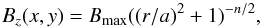 (1)with r2 = x2 + y2, where x,y are the two orthogonal horizontal spatial coordinates and a defines a characteristic radius of the polarity. Bz is maximum at r = 0 and decreases as r− n for r ≫ a.
The case n = 3 corresponds to a magnetic source located at z = −a below the photosphere; it models the linear spreading with height, above z = −a, of a thin flux tube located below z = −a (see appendix of Demoulin et al. 1994). Field distributions like this were used to model the magnetic field of ARs by using a series of flux concentrations with the parameters (position and intensity) fitted to the observed magnetograms. This allowed the computation of their coronal magnetic topology. In particular, the derived intersections with the chromosphere of the computed separatrices were found close to the observed flare ribbon locations, showing that magnetic reconnection is responsible for the energy release (e.g., Gorbachev & Somov 1988; Mandrini et al. 1995; Longcope 2005).
Next, we computed the probability  of having a magnetic field value of Bz ± dBz/ 2 within the magnetic polarity. This probability corresponds to the area 2πr dr with r related to Bz by Eq. (1). Differentiation of Eq. (1) provides
  (2)By substituting Eq. (2) into
  we obtain
  (3)The proportionality constant is found by setting the total probability to unity. This integral is calculated in the r-range [0,rmax] corresponding to the Bz-range [Bz,max,Bz,min]. This gives
 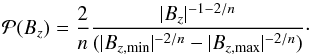 (4)This result extends approximately to a series of flux concentrations modelling an AR as long as the source fields do not overlap significantly. For n = 3, representing a magnetic source,
  , producing a slope of −1.67 when plotting
  against Bz on a log-log plot. At the limit of very high n values
  , as for the diffusion case of one polarity (cf. Sect. 2.2 and Eq. (8)). Although there is no clear physical interpretation of this, it is unsurprising that differing Bz distributions, which depend on two spatial dimensions x and y, can produce the same , which varies as a function of only one variable, namely Bz.
2.2. Diffusion of a magnetic polarity
Already during the emergence, and even more so during the decay phase, the AR magnetic field is affected by convective cells at various spatial scales (i.e. by granules and supergranules). The AR magnetic field is progressively dispersed in an ever increasing area nearly proportional to the time duration since the emergence started (e.g., van Driel-Gesztelyi et al. 2003). This is the behaviour expected with classical linear diffusion. However, the dispersion of an AR also involves local mechanisms not included in classical diffusion, such as clustering of the field at the border of convective cells, cancellation of opposite-sign polarities, and submergence of small-scale loops. Classical diffusion can provide an explanation of the area evolution, but can it also explain the observed magnetic field distribution?
The classical diffusion of the vertical field component Bz(x,y,t) is governed by 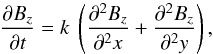 (5)where k is a constant coefficient and t is time.
For a concentrated initial field with one polarity of magnetic flux F, the solution of Eq. (5) is 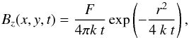 (6)with r2 = x2 + y2.
As in Sect. 2.1, we computed the probability of having a magnetic field value of Bz ± dBz/ 2 within the magnetic polarity, which again corresponds to an area 2πr dr. In this case, r is related to Bz with Eq. (6). Differentiation provides 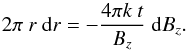 (7)Normalisation by the total probability in the Bz-range [Bz,max,Bz,min] gives
 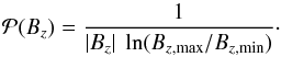 (8)When is plotted against Bz in a log-log plot, a slope of −1 is produced.
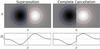 |
Fig. 1 Two different scenarios for flux dispersion of a bipole as described in Sect. 2.3. The left-hand side of the plot shows superposition with no cancellation, and the right-hand side shows the case where complete cancellation occurs at x = 0. Two isocontours are also shown for the negative and positive spots. The two plots in the bottom row show a cross section of the magnetic field values taken at y = 0. |
2.3. Diffusion of a magnetic bipole
In this subsection we consider the evolution of a simple bipole to model the global evolution of an AR. We assume that the centres of the two polarities are located at the fixed positions x = ± R,y = 0. Since Eq. (5) is linear in Bz, the evolution of the bipole is the superposition of two solutions of Eq. (6) when shifted spatially by ± R:  (9)where F is the total flux of the isolated positive polarity. This is illustrated in the top left panel of Fig. 1, with the bottom left panel showing a cross section of the Bz values taken at y = 0.
The spatial distribution of Bz in Eq. (9) depends on the parameters F,  and R. F defines the field strength, while a defines the polarity size, and both are scaling factors. The main parameter of Eq. (9) is R/a. For R/a ≫ 1 the polarities are well separated and do not overlap, while for R/a ≪ 1 the opposite polarities mostly cancel each other, leaving a dipolar magnetic field.
The probability distribution of Bz is computed numerically since the Bz isocontours are not simply circles ( is computed by summation along these isocontours). In a log-log plot, the slope is in the range [−1,−0.94] at all times during the diffusive evolution (Fig. 2). More precisely, the slope ≈−1 for R/a> 3 and converges rapidly to −1 when the separation between the polarities is larger, as expected from Eq. (8). The slope is maximum, ≈−0.94, for 1 ≤ R/a ≤ 1.7, while it shows a slight decrease to ≈−0.96 for lower R/a values. When the polarities are interacting, the slope is slightly less steep than with one polarity (slope =−1) because the other source acts to decrease Bz and even removes weak values surrounding the inversion line. This implies fewer cases with a given Bz value, particularly for low Bz, making the global slope of the distribution slightly less steep. Finally, the increase in probability values with time, as seen in Fig. 2, is due to the normalisation of the total probability to 1, while the maximum of Bz decreases with time and the minimum of Bz is selected to be fixed (here to Bz = 1); in this way, we modelled an instrumental detectability threshold.
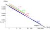 |
Fig. 2 Log-log plot of the probability distribution of Bz versus Bz for a bipolar field diffusing with time. The Bz spatial distribution is described by Eq. (9). The time t is normalised by the initial time when R/a = 1 is selected (blue line). Only Bz> 1 is supposed to be detectable. The black straight line has a slope −1 for reference. |
The net flux evolution is computed by performing the integration on the positive polarity, where x> 0, which gives, 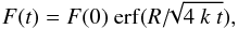 (10)where erf is the error function
  . For short diffusion times,
  , F(t) is nearly constant, while for long diffusion times, Eq. (10) can be approximated as
  so that the flux of the polarities decreases as t−1/2. The cancellation of flux is due to the superposition of the opposite polarities in the x direction. This is a 1D process, which means that it scales as the ratio of the sizes in the x direction:
  .
.
Equation (9) describes the diffusion of each polarity isotropically, that is, they do not cancel but are spatially superposed. This implies an apparent loss of magnetic flux by superposition of opposite Bz values when computing the total flux, but there is no physical cancellation since the full amount of both polarities continues to diffuse with time. The other extreme behaviour, a complete cancellation at the inversion line, can be described by the field 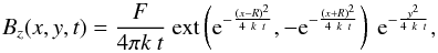 (11)where the function ext(a,b) is defined as a if |a| > |b|, b if |a| < |b|, and 0 otherwise (then it is a signed extremum function except at |a| = |b| , where it vanishes to model immediate cancellation). This scenario is shown in the top right panel of Fig. 1, with the bottom right panel showing the Bz values at y = 0.
Equation (11) describes two magnetic polarities that are diffusing independently of each other (no overlap of Bz as in Eq. (9)), and they exactly cancel at x = 0 (no diffusion in the region of the other polarity). In the photosphere the opposite polarities diffuse into each other as a result of advection by convective cells of small flux tubes, which at some point meet and cancel. This process is mostly driven by the supergranular flows, and the typical distance of travel across the inversion line in the other polarity (the mean free path) is expected to be of the order of a supergranular cell (about 30 Mm). Equations (9) and (11) are the limits when the mean free path is infinite and zero, respectively.
The probability of Bz, for values where the corresponding isocontour does not touch the inversion line (x = 0), given by Eq. (11), has the same Bz dependence as Eq. (8). For the lower Bz values, some of the pixels are absent (those that would be located on the other side of the y axis if they had not undergone cancellation), therefore the probability is slightly lower. In summary, the distribution shown in a log-log plot (as in Fig. 2) has a slope of exactly −1 for high |Bz| values and slightly above −1 (less steep) for low |Bz| values.
All in all, this implies that is similar for an inefficient cancellation rate (Eq. (9)) and for a very efficient one (Eq. (11)). Thus, any cancellation rate, with a classical diffusion of the polarities, is expected to imply a slope ≳−1 for drawn in a log-log plot.
3. Data and AR selection
3.1. Data and data treatment
We studied the magnetic field evolution of 37 ARs that emerged on the solar disk between June 2010 and the end of 2014. To ensure consistency and correct identification of the emergence time, only those ARs that emerged in relatively magnetic-field free regions (without detectable remnant of other ARs) were chosen. In addition, only ARs emerging before the central meridian passage (CMP) were selected to analyse the entire, or at least most of, the emerging phase. The resulting ARs are listed in Table A.1.
The ARs were studied using photospheric line-of-sight magnetograms from the Helioseismic Magnetic Imager (HMI; Schou et al. 2012) on board the Solar Dynamics Observatory (SDO; Pesnell et al. 2012). The time at which each AR started to emerge was found by visual inspection of the line-of-sight magnetograms. Although this method is subjective and is influenced by the position of the AR on the solar disk (these problems are discussed in Fu & Welsch 2016), these effects were negligible as a result of the relatively low time-cadence data (six hours) used here to study the ARs.
For the decaying ARs discussed in Sect. 5.3, the ARs began to emerge on the far side of the Sun. To estimate the emergence start times in these cases, we used data from the Extreme UltraViolet Imager (EUVI) telescope on board the Solar Terrestrial Relations Observatory Behind (STEREO B; Kaiser et al. 2008) spacecraft.
The magnetic field data were first treated using a cosine correction assuming that the magnetic field is locally vertical. This was followed by a derotation to central meridian to correct for area foreshortening.
3.2. Definition of AR area
A rectangular submap surrounding the largest extent of the AR was manually defined, with the area of the AR itself defined using a semi-automated technique (adapted from that outlined in Yardley et al. 2016). This process was important to ensure an unbiased estimation of the field distribution of the AR, especially as the rectangular submap contained magnetic field from the quiet Sun as well as possibly flux from neighbouring regions, which would have affected the results.
To focus on the larger-scale features rather than individual flux fragments, the absolute values of the magnetic field within the submap were smoothed using a Gaussian filter with a standard deviation (width) of 7 pixels. The AR extension was then automatically defined from the areas in which the pixels had smoothed values >40 G (shown in Fig. 3a). For the initial stages of flux emergence, our code searched for a bipolar region, defined as having between a fifth and five times the amount of positive flux as negative flux. When no bipole was found, a search was made for positive and negative bubbles that were close to each other (within a distance of 20 pixels, approximately 10 arcsec). To include regions of fragmented flux emergence, more of the original bubbles were accepted if they lay within 20 pixels of this selection or 10 pixels of these additional bubbles.
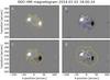 |
Fig. 3 Example of the area selection and dilation procedure (Sect. 3.2) for NOAA AR 11945. Panel a) shows the selection >40 G in the blurred map of absolute field values. Panel b) shows the selection >20 G and <−20 G in the smoothed signed map (blue), along with the selection from panel a (yellow). Panel c) shows the selection after the field-dependent dilation, and panel d) the final region selection after the field-independent dilation. |
As ARs evolve, they change significantly, with the sea-serpent structures coalescing into two main polarities that grow to cover a larger area of the solar surface. To reflect these changes, the AR area selection criteria were changed after the unsigned flux of the near bipole region reached 8 × 10²⁰ Mx, when the AR area was found to dominate the rectangular submap. The AR area was still chosen from the regions of pixels with smoothed values >40 G, but the selection criteria were different, with larger regions and regions close to the large regions being chosen. To capture fragments of flux that had broken away from the main polarities, this area was then extended to neighbouring regions (within 10 pixels).
If at any time step the automated selection was not satisfactory, for example if there were inconsistencies between neighbouring time steps (i.e. flux at the edge of the region was not included in the selection at one time step, but was included in both the preceding and the following time steps), then the selection could be made manually from the smoothed submap.
After the region had been selected, dilations were applied to include the region immediately surrounding the selection, as this was found to have a different magnetic field distribution to that of the quiet Sun (see Sect. 5.5) and was therefore considered to be strongly influenced by the emerging flux. For the first dilation, the signed data were smoothed using a Gaussian filter of width 7 pixels. The pixels of smoothed values >20 G or <−20 G were selected (shown in Fig. 3b with blue contours). Each of these regions was compared to the previously selected region (yellow contour), and when some overlap was found, the pixels in that region were unmasked (panel c of Fig. 3). Because the blurring was applied to the signed values, the dispersing parts of the region were likely to be accepted, while any diffuse neighbouring regions of opposite polarity should have been avoided. Finally, two field-independent dilations were applied, both using a disk-shaped kernel with a radius of 12 pixels (providing a smoother edge than a single dilation with a larger kernel). All the pixels in the dilated region (shown Fig. 3d) were analysed.
4. Kernel density estimation analysis
4.1. Method
Kernel density estimation plots (KDEs; Wegman 1972; Silverman 1986, and references therein) were created for each time step, showing the distribution of pixels with respect to the field value (flux density) on a log-log scale. KDEs are very similar to histograms in that both types of plots show the distribution of data points. However, histograms rely on discretising the data points, using user-defined bins, which normally leads to a loss of information. Moreover, the arbitrary choice of bin positions can affect the subsequent interpretation. On the other hand, KDEs assign a kernel of a certain width to each data point, effectively smoothing the finite number of data points. This KDE technique has been shown to be superior to histograms both theoretically and in applications (e.g., de Jager et al. 1986; Vio et al. 1994), and KDEs have been used in a broad range of astrophysics domains (e.g., Schulze-Hartung et al. 2012; Sui et al. 2014).
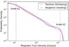 |
Fig. 4 Field distribution of NOAA AR 11945 18 h after the start of its emergence. The distribution is calculated from the pixels within the contour shown in panel d of Fig. 3. The positions of the knees, k1 and k2 (vertical lines), and the lines of best fit to the middle section (dashed) are shown for both polarities. |
The applied kernels of KDE plots can take on any shape and were chosen to peak at the data point value and to decay away from this. The kernel widths can also be varied depending on the data point value. A larger width can be used where there are fewer data points, enabling the noise in the distribution to be made roughly constant. While the smoothness of a KDE clearly depends on the kernel widths, similar to the dependence of histograms on their bin widths, unlike histograms there is no dependence on an arbitrary choice of bin position (the kernel is applied and centred on each data point).
The KDEs in this study1 were created using a Gaussian kernel with standard deviation equal to 2.5 G for field values between −25 and +25 G and equal to |Bz| /10 for |Bz| > 25 G. This was chosen to create a plot whose noise level was roughly independent of Bz (as it would appear on a log-log plot). From the theoretical considerations of Sect. 2, a line with a slope of −1 would be expected for the KDE when plotted on a log-log scale. This means that the pixel frequency would be proportional to 1/ |Bz|. The optimal KDE should be built with a variable kernel width such that the kernel width is inversely proportional to the frequency at that point. A kernel width proportional to |Bz| was therefore used. There are a few reasons why a lower limit on the kernel width was chosen for low |Bz| values. One reason is to represent the instrumental errors, which reduce the precision of the measurement. Another reason is that the frequency does not increase indefinitely as the value |Bz| decreases. Instead, it is expected that the distribution and its derivative are continuous across 0 Gauss on a linear Bz scale. The KDE plots show that the distributions are flatter for |Bz| values lower than ~25 G (e.g., Fig. 4).
4.2. Observed distributions
All the KDEs were found to have some common features, namely a flatter section below ~10 G followed by a turning point (the first knee, at field value k1, indicated by a vertical line in Fig. 4), a steeper section up to ~1000 G, and then another turning point (the second knee, at field value k2, also indicated by a vertical line) after which the frequency drops off rapidly. Although k2 varies greatly with the age and strength of the AR, it was not used to characterise the distribution as it is highly dependent on only a very small proportion of pixels.
To capture only the larger-scale features, an additional smoothed KDE plot was created using Gaussian kernels of twice the width as before, and the positions of the knees (k1 and k2) were found from this. k1 was taken as the point of most negative second derivative before the slope reaches values lower than −1. k2 was taken as the first time, moving along the KDE graph from right to left, that the slope becomes more positive (less steep) than −3. A best-fit line was fitted to the original (not extra smooth) KDE plot between 1.5 × k1 and  . The best-fit line was calculated using the method of least squares, taking data points evenly spaced along the log(B) axis. Examples are shown (dashed lines) in Fig. 4 for both the positive and negative distributions.
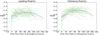 |
Fig. 5 Slope of the best-fit straight line to the middle section of the log-log field distribution plot, calculated as illustrated in Fig. 4. This plot shows each slope value plotted against the age of the AR from the start of its emergence (t = 0) at each time step and for each AR. Data for leading and following sunspots were separated. Second-order polynomials were least-squares fitted; they show the general trend. |
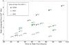 |
Fig. 6 Peak unsigned flux reached by each AR plotted against the time it took to reach that value from the start of the emergence. The size of the points indicates the area covered by the region at that time. The points are labelled with their NOAA AR number. |
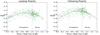 |
Fig. 7 Similar to Fig. 5, this plot shows the evolution of the slope. Here, the slope is plotted against a function of the normalised magnetic flux. This normalised flux is defined as the ratio of the AR flux to the peak flux that region achieves. The peak flux and the ratios are found separately for the positive and negative magnetic polarities. To distinguish between emergence and decay phases, the function f(F), defined by Eq. (12), is used in abscissa. The emergence phase is in the range [0,1] and the decay phase is for abscissa >1. Second-order polynomials were least-squares fitted; they show the general trend. |
5. Observational results
5.1. Temporal evolution
Figure 5 shows the change in slope of the distributions with time from the start of AR emergence for all studied ARs (listed in Table A.1). The slopes start off steep and negative, in about the range [−2.2,−1.5], peak in the range [−1.7,−1.2], and then become steeper (more negative) again as the ARs decay.
The initially steep slope is related to the fragmented emergence. It is followed by the coalescence of flux elements to form stronger flux concentrations, and the slopes around t = 60 h are comparable to the slopes found for a magnetic source with n = 3 (≈−1.67) as derived in Sect. 2.1, Eq. (4). The change in slope during the regions’ decay is due to dispersion with the number of higher-field pixels decreasing and the proportion of low- to medium-field pixels increasing. The latter evolution goes away from the slope given by classical diffusion (≈−1, Sect. 2.3).
5.2. Evolution versus magnetic flux
The emergence timescale varies broadly from one AR to another (e.g., van Driel-Gesztelyi & Green 2015,and references therein). As a result, in Fig. 5 ARs with various flux values and emergence durations are presented together, which mixes different phases and field strength distributions of AR evolution (e.g., ~80 h after the start of flux emergence some ARs are still emerging, while smaller ARs are already in their decay phase). In this section, we characterise the emergence stage of an AR by the amount of emerged magnetic flux, normalised to its maximum value.
The maximum flux, Fmax, is defined as the maximum unsigned flux achieved during the AR evolution, so long as this value was not reached at the last time step. Twenty-four regions of the original thirty-seven reached peak flux and were included in this part of the study. The other regions were still in their emergence phase at the end of the observational time period.
Figure 6 shows that larger ARs generally take a longer time to emerge, but the relationship between emergence time and peak flux is not simple, with some regions taking a long time to emerge without reaching a particularly high peak flux. The rates of flux emergence were seen to vary, both during the emergence of single regions and from one AR to another, in agreement with the results of Poisson et al. (2015, 2016) obtained on other sets of ARs. Some regions were seen to have an initial gradual emergence phase followed by a more rapid phase, while others emerged rapidly at the start and had a decreasing emergence rate later on.
The ratio of flux to peak magnetic flux is used in Fig. 7 to study the emergence independent of the time it takes. Here the maximum flux is computed separately for the two magnetic polarities. Moreover, to separate the emergence from the decay phase (which is in the same range of flux), we used the function f(F) defined as ![Mathematical equation: \begin{eqnarray} f(F/F_{\rm max}) &= F/F_{\rm max} \qquad \,\,\, \mbox{\rm for } t\leq t_{\rm max} \label{eq_flux}\\[3mm] &= 2-F/F_{\rm max} \quad \mbox{\rm for } t>t_{\rm max} , \nonumber \end{eqnarray}](/articles/aa/full_html/2016/12/aa28948-16/aa28948-16-eq100.png) (12)where t is the time since the start of emergence, Fmax is the maximum flux, and tmax the duration of the emergence until Fmax is reached. Although several problems arise as a result of the variable emergence rates, Fig. 7 shows an improvement to Fig. 5 in that the trends, particularly in the case of the leading spot, are more pronounced.
(12)where t is the time since the start of emergence, Fmax is the maximum flux, and tmax the duration of the emergence until Fmax is reached. Although several problems arise as a result of the variable emergence rates, Fig. 7 shows an improvement to Fig. 5 in that the trends, particularly in the case of the leading spot, are more pronounced.
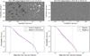 |
Fig. 8 Decayed AR (top left) and quiet Sun region (top right), with their magnetic field distributions in the bottom left and right panels, respectively. The positions of the knees, k1 and k2 (vertical lines), and the lines of best fit to the middle section (dashed) are shown for both polarities. |
On average, the slopes of the field distribution between the leading and following polarities vary. At the beginning of the emergence phase, the field distribution slope is slightly more negative for the following than the leading polarity, becoming less negative as the peak flux value is reached. However, these differences, best seen in the fitted polynomials, are comparable to the standard deviation of the residuals. To reduce the statistical noise and investigate whether these slopes are dependent upon parameters other than the normalised flux, a larger sample of regions would need to be studied.
In summary, Fig. 7 shows one important aspect of the evolution of the magnetic field distribution, namely the transformation of a distribution mainly dominated by the weak fields (steeper slope) at the beginning of emergence, to one with more numerous stronger field pixels around the maximum flux, and then back to a distribution dominated by weak-field pixels. The typical slopes around the maximum flux correspond to the slope found with the simple model described in Sect. 2.1. In contrast, neither the initial emergence nor the decay phase conforms with the plausible theoretical model we considered. In particular, the distribution during the beginning of the decay shows an evolution opposite to that expected from classical diffusion (with the slope becoming steeper rather than tending towards the expected value −1 as found in Sect. 2.3).
5.3. Decayed ARs
The ARs selected for this study were those that emerged on the solar disk and were tracked until they rotated too far (≥60°) from the central meridian. Therefore all the data came from relatively young ARs that were 6 days old at most. A preliminary study of decaying ARs was performed to determine whether the decreasing slope trend continues as ARs continue to age. Three relatively isolated decaying ARs (NOAA 12165, 12176, and 12414), in which no new flux emergence was observed, were selected. The ARs were chosen to be of approximately the same maximum flux (~5 × 10²¹ Mx), as this affects how quickly the ARs decay and how quickly their distribution changes. Two of these ARs started emerging on the far side of the Sun, so their emergence start times were identified by eye using 171 Å data from STEREO B. Two of the regions were observed for multiple solar rotations and provided data points at later times.
To calculate the field distributions of these regions, all of the pixels within a rectangular subplot centred on the AR were used. This simple procedure was used because at these times the ARs are quite dispersed and difficult to distinguish from the quiet-Sun field. An example of one of the decaying ARs and the rectangular subplot that defined the region is shown in the top left panel of Fig. 8, with the AR field distribution shown in the bottom left panel. The slopes of the three decaying ARs at the different times since they started emerging are shown in Fig. 9. Here, an average of the positive and negative slope values was used, as the slopes for the two different polarities were consistently very similar; they differed by less than 0.1 in each case. This may be different for an AR where the leading polarity retains a coherent spot for longer than the following polarity.
The results shown in Fig. 9 indicate that the downward (steepening) trend of the slope during AR decay continues as the regions continue to age. A deeper study is needed to confirm this result and to determine the dependence on maximum flux.
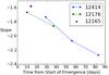 |
Fig. 9 Slopes for older decaying ARs shown against time from the start of the AR emergence. A downward trend can be seen. |
5.4. Quiet Sun
At the end stages of AR decay, the dispersing magnetic field becomes part of the quiet Sun. We studied four regions to determine the slope of the quiet-Sun field distribution. As for the decaying ARs in Sect. 5.3, all the pixels within a selected rectangular area were used to build the field distribution. One of the four regions and its distribution is shown as an example in the right column of Fig. 8. The regions studied were taken at central meridian on 2010-May-25 (shown in Fig. 8), 2015-Nov.-25, 2015-Dec.-22 and 2016-Jan.-18. The latter three regions were centred on −75 arcsec in solar Y.
The average of the positive and negative distribution slopes were −3.0, −3.0, −2.9, and −3.3, with the difference between the positive and negative being less than 0.3 for each region. When we combine this result with that of Fig. 9, it implies that the slope of the AR field distribution continues to decrease (steepen) as the AR decays, until it reaches the quiet-Sun value ~−3.
A possible origin of this ~−3 slope is the advection of the magnetic field by the diverging flow of supergranules, as follows. With an axisymmetric magnetic field and purely radial flow at speed ur away from the cell centre, the ideal induction equation in the stationary regime implies that Bz(r) ∝ 1/(rur), with r being the radial distance away from the cell centre. When we assume that ur is nearly independent of r away from the cell centre and boundary, this implies that Bz ∝ 1 /r. Compared to Eq. (1), this provides n ≈ 1 for r ≫ a, which produces a slope of −3 from Eq. (4). This rough approach assumes a very simple form for the convective flow and does not include other important physical processes such as the field concentration or cancellation at the cell boundary. A detailed analysis of observations and/or numerical simulations will be needed to test if the ~−3 slope found in the quiet Sun is mainly due to the advection of the magnetic field by the diverging flow of supergranules.
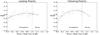 |
Fig. 10 Similar to Fig. 7, but in this case only using data points from ARs within 10 h, ~6 degrees, of their central meridian passage. To distinguish between emergence and decay phases, the function f(F), defined by Eq. (12), is used in the abscissa. Second-order polynomials were least-squares fitted; they show the general trend. |
5.5. Possible problems for the derived distributions
In this section we report some of the tests done to ensure that the derived slopes in emerging ARs are not affected by the inclusion of surrounding quiet Sun or by projection effects.
With regard to the area selection process (as described in Sect. 3.2), we analysed the area bordering the ARs by selecting a ribbon-like region around the ARs and by studying the field distributions for various ribbon thickness. In the bordering region we found a distribution that differed from that of the quiet Sun. We therefore decided to include these neighbouring pixels in the selection by applying dilations. Care was taken to ensure that the dilations were not too large to avoid including decaying field from old ARs nearby, which could be identified by eye.
The quiet-Sun region was also used to study possible effects arising from the position of the region on the solar disk with respect to distance from the central meridian because we used line-of-sight magnetic field data. In contrast to ARs, the distribution of the quiet Sun is expected not to evolve on a timescale of weeks, so that any observed change in the observed distribution indicates a viewing point bias as the region shifts away from the central meridian. The main change found in the distribution was a shift of k1 to higher field values. One reason for this are the larger errors in the line-of-sight magnetic field measurement closer to the solar limb (Hoeksema et al. 2014). These errors are then exaggerated by the cosine correction under the radial field assumption. Even if there were no errors in the measured field values, the validity of the assumption that the measurements are of a purely radial field decreases for both low field-strength regions (a less vertical magnetic field) and away from the disk centre, where the measured field contains a larger component of the transverse field. This also introduces errors in the field distribution.
A shift in k1 has implications for the slope, with a larger k1 in general giving rise to a steeper slope. The shift in k1 becomes more pronounced ~3–4 days from central meridian (~45–60 degrees). In the AR sample analysed in Sects. 5.1 and 5.2, if k1 was seen to increase significantly as the region moves away from the central meridian, then this and any following time steps were removed from the analysis.
To further ensure that the trends seen in Figs. 5 and 7 did not result from the position of the AR on the disk in terms of area-foreshortening effects and interpolations associated with derotation, Fig. 10 includes only data from ARs within 10 h, ~6 degrees, of their central meridian passage. The regions were in various stages of their evolution as they passed central meridian. Figure 10 shows the same trends as were obtained with the larger number of data points in Fig. 7, with a slightly more marked difference between the leading and following polarities. We therefore conclude that the trends in slope are related to the real field distributions of the ARs.
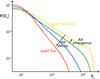 |
Fig. 11 Schema summarising the evolution of the Bz distribution with a log-log plot. It shows the difference in the distribution between a newly emerging AR (green), one at around the time of peak flux (yellow), and one during the decay phase (blue). After this time, the field distribution of the AR evolves towards that of the quiet Sun (red). Since both magnetic polarities have very similar distributions at a given time (e.g., Figs. 4 and 8), they are not separated in this schema. |
6. Discussion and conclusions
In this study of 37 emerging ARs, we have shown that there is a relationship between the slope of the vertical component of the photospheric field distribution and the age of an AR. This is summarised in Fig. 11. At the beginning of a region emergence, the slope is steep and negative. The slope becomes less steep, which indicates the coalescence of the fragmented flux that emerges. Later, the slope reaches a maximum just before the region achieves its peak flux value (at ~0.75–0.8 peak flux), before the decay processes become dominant. The slope becomes more negative as the region disperses, and this decreasing trend continues towards the quiet-Sun slope value of ~−3 (Fig. 8).
A comparison between the observational and theoretical results showed that a simple model of magnetic concentrations can describe the field (flux density) distribution in emerging ARs during the coalescence phase when smaller flux concentrations merge to form larger ones, leading to sunspot formation. The model predicts a slope of ≈−1.67 for n = 3, in good agreement with the slope values found in observations of the coalescence phase (Figs. 5 and 7).
However, later on there is a major deviation from the classical-diffusion model in the decay phase, indicating that AR magnetic fields do not disperse by simple diffusion. The latter predicts that after reaching peak flux, the field strength distribution should be characterised by a slope that evolves from the range [−1.6,−1.4] towards the diffusion exponent value of −1. However, as Figs. 7 and 10 clearly demonstrate, once ARs pass their peak flux and start decaying, their field strength distribution slopes evolve quite differently from these expectations: they start to attain higher negative values. Furthermore, ARs measured in the later decay phase display slopes in the range of [−2.3,−1.6], as shown in Fig. 9, while the quiet Sun, which can be regarded as the end-product of AR decay, shows a slope ≈−3. How can we understand this behaviour, which is so clearly opposite to the classical diffusion scenario?
We suggest that magnetic flux reprocessing by convective cells is responsible for the observed evolution of field distributions. Magnetic flux is being gnawed away by granular and supergranular convective cells, in agreement with the turbulent diffusion model (e.g., Petrovay & Moreno-Insertis 1997), which carry away flux concentrations from the strong-field area of ARs. Petrovay & van Driel-Gesztelyi (1997) analysed various theoretical models of sunspot decay using observational data of umbral areas and found that the turbulent diffusion model was the only model supported by the data. The turbulent diffusion model is also consistent with the removal of AR magnetic field by moving magnetic features (e.g., Kubo et al. 2008), the movement of which is a result of convective flows. The advected field fragments become concentrated along the boundaries of supergranular cells, where they occasionally meet and cancel with opposite-polarity field. The cancelled flux submerges and is re-processed by convection. Part of the reprocessed flux emerges in the centre of supergranular cells as weak intranetwork flux. This process breaks up strong-field flux tubes and causes them to emerge as weaker field, which effectively transfers strong field to weak field in the field distribution of a decaying AR and causes the slope of the field distribution to steepen (becoming more negative). The weak intranetwork field is carried to the boundary of the supergranular cells and becomes more concentrated there, which is a counter-mechanism to the former scenario. We propose that the −3 slope found in the quiet-Sun field is the result of the combination of these two mechanisms.
Although the evolution of the magnetic field in a decaying AR is very different from what is expected in classical diffusion (slope of −1), the AR area has previously been found to increase approximately linearly with time (e.g., van Driel-Gesztelyi et al. 2003), in accordance with the classical diffusion model. Is there a contradiction here? We propose that the increase of AR area is due to the non-stationarity of the supergranular convective cells, which have a lifetime of about one day. This non-stationarity creates a random walk of the flux tubes, which is the underlying physics of classical diffusion. Therefore the AR evolution can be seen as classical diffusion regarding area increase, while the magnetic field distribution is governed by magneto-convection. These ideas have to be tested in simulations of emerging ARs with and without magneto-convection.
Other studies (e.g., Abramenko & Yurchyshyn 2010) have characterised the active region magnetic field by its degree of intermittency. It could be interesting to compare this with changes in the field distribution slopes as the resolution of the magnetogram is decreased and particularly for resolutions that do not resolve the highly intermittent small-scale structure.
The code used to create and analyse KDEs in this study is available here: https://github.com/SallyDa/Sally_KDE
Acknowledgments
The authors are grateful to Mark Linton for the interesting discussions and the referee for their insightful comments. We are thankful to the SDO/ HMI and AIA consortia for the data. This research has made use of SunPy, an open-source and free community-developed solar data analysis package written in Python (SunPy Community et al. 2015). S.D. and S.L.Y. acknowledge STFC for support via their Ph.D. studentships. Both D.B. and L.v.D.G. are funded under STFC consolidated grant numbers ST/H00260X/1 and ST/N000722/1. L.v.D.G. also acknowledges the Hungarian Research grant OTKA K-109276. D.M.L. is an Early-Career Fellow funded by the Leverhulme Trust. D.P.S. is funded by the US Air Force Office of Scientific Research under Grant No. FAQ550-14-1-0213.
References
- Abramenko, V., & Yurchyshyn, V. 2010, ApJ, 722, 122 [NASA ADS] [CrossRef] [Google Scholar]
- Cheung, M. C. M., & Isobe, H. 2014, Liv. Rev. Sol. Phys., 11 [Google Scholar]
- Cheung, M. C. M., Rempel, M., Title, A. M., & Schüssler, M. 2010, ApJ, 233 [Google Scholar]
- de Jager, O. C., Raubenheimer, B. C., & Swanepoel, J. W. H. 1986, A&A, 170, 187 [NASA ADS] [Google Scholar]
- Demoulin, P., Mandrini, C. H., Rovira, M. G., Henoux, J. C., & Machado, M. E. 1994, Sol. Phys., 150, 221 [NASA ADS] [CrossRef] [Google Scholar]
- Fan, Y. 2001, ApJ, 554, L111 [NASA ADS] [CrossRef] [Google Scholar]
- Fu, Y., & Welsch, B. T. 2016, Sol. Phys., 291, 383 [NASA ADS] [CrossRef] [Google Scholar]
- Gorbachev, V. S., & Somov, B. V. 1988, Sol. Phys., 117, 77 [NASA ADS] [CrossRef] [Google Scholar]
- Gošić, M., Bellot Rubio, L. R., Orozco Suárez, D., Katsukawa, Y., & del Toro Iniesta, J. C. 2014, ApJ, 797, 49 [NASA ADS] [CrossRef] [Google Scholar]
- Harvey, K., & Harvey, J. 1973, Sol. Phys., 28, 61 [NASA ADS] [CrossRef] [Google Scholar]
- Hathaway, D. H., & Choudhary, D. P. 2008, Sol. Phys., 250, 269 [NASA ADS] [CrossRef] [Google Scholar]
- Hoeksema, J. T., Liu, Y., Hayashi, K., et al. 2014, Sol. Phys., 289, 3483 [Google Scholar]
- Kaiser, M. L., Kucera, T. A., Davila, J. M., et al. 2008, Space Sci. Rev., 136, 5 [NASA ADS] [CrossRef] [Google Scholar]
- Kubo, M., Lites, B. W., Shimizu, T., & Ichimoto, K. 2008, ApJ, 686, 1447 [NASA ADS] [CrossRef] [Google Scholar]
- Longcope, D. W. 2005, Liv. Rev. Sol. Phys., 2 [Google Scholar]
- Mandrini, C. H., Demoulin, P., Rovira, M. G., de La Beaujardiere, J.-F., & Henoux, J. C. 1995, A&A, 303, 927 [NASA ADS] [Google Scholar]
- Pariat, E., Aulanier, G., Schmieder, B., et al. 2004, ApJ, 614, 1099 [Google Scholar]
- Parnell, C. E., DeForest, C. E., Hagenaar, H. J., et al. 2009, ApJ, 698, 75 [NASA ADS] [CrossRef] [Google Scholar]
- Pesnell, W. D., Thompson, B. J., & Chamberlin, P. C. 2012, Sol. Phys., 275, 3 [NASA ADS] [CrossRef] [Google Scholar]
- Petrovay, K., & Moreno-Insertis, F. 1997, ApJ, 485, 398 [NASA ADS] [CrossRef] [Google Scholar]
- Petrovay, K., & van Driel-Gesztelyi, L. 1997, Sol. Phys., 176, 249 [NASA ADS] [CrossRef] [Google Scholar]
- Poisson, M., Mandrini, C. H., Démoulin, P., & López Fuentes, M. 2015, Sol. Phys., 290, 727 [NASA ADS] [CrossRef] [Google Scholar]
- Poisson, M., Démoulin, P., López Fuentes, M., & Mandrini, C. H. 2016, Sol. Phys., submitted [Google Scholar]
- Schou, J., Scherrer, P. H., Bush, R. I., et al. 2012, Sol. Phys., 275, 229 [Google Scholar]
- Schulze-Hartung, T., Launhardt, R., & Henning, T. 2012, A&A, 545, A79 [NASA ADS] [CrossRef] [EDP Sciences] [Google Scholar]
- Silverman, B. W. 1986, Density estimation for statistics and data analysis, Vol. 26 (CRC Press) [Google Scholar]
- Strous, L. H., Scharmer, G., Tarbell, T. D., Title, A. M., & Zwaan, C. 1996, A&A, 306, 947 [NASA ADS] [Google Scholar]
- Sui, N., Li, M., & He, P. 2014, MNRAS, 445, 4211 [NASA ADS] [CrossRef] [Google Scholar]
- SunPy Community, Mumford, S. J., Christe, S., et al. 2015, Computational Science and Discovery, 8, 014009 [Google Scholar]
- Toriumi, S., & Yokoyama, T. 2011, ApJ, 735, 126 [NASA ADS] [CrossRef] [Google Scholar]
- van Driel-Gesztelyi, L., & Green, L. M. 2015, Liv. Rev. Sol. Phys., 12, 1 [NASA ADS] [CrossRef] [Google Scholar]
- van Driel-Gesztelyi, L., Mandrini, C. H., Thompson, B., et al. 1999, in Third Advances in Solar Physics Euroconference: Magnetic Fields and Oscillations, eds. B. Schmieder, A. Hofmann, & J. Staude, ASP Conf. Ser., 184, 302 [Google Scholar]
- van Driel-Gesztelyi, L., Démoulin, P., Mandrini, C. H., Harra, L., & Klimchuk, J. A. 2003, ApJ, 586, 579 [NASA ADS] [CrossRef] [Google Scholar]
- Vio, R., Fasano, G., Lazzarin, M., & Lessi, O. 1994, A&A, 289, 640 [NASA ADS] [Google Scholar]
- Wegman, E. J. 1972, Technometrics, 14, 533 [CrossRef] [Google Scholar]
- Yardley, S. L., Green, L. M., Williams, D. R., et al. 2016, ApJ, 827, 151 [NASA ADS] [CrossRef] [Google Scholar]
- Zwaan, C. 1978, Sol. Phys., 60, 213 [Google Scholar]
Appendix A: Table of ARs
Thirty-seven ARs that emerged on the solar disk between June 2010 and the end of 2014 were studied and are listed in the
following table. These ARs emerged in regions relatively free of magnetic field before (or around) their central meridian passage.
Characteristics of the studied ARs.
All Tables
All Figures
|
Fig. 1 Two different scenarios for flux dispersion of a bipole as described in Sect. 2.3. The left-hand side of the plot shows superposition with no cancellation, and the right-hand side shows the case where complete cancellation occurs at x = 0. Two isocontours are also shown for the negative and positive spots. The two plots in the bottom row show a cross section of the magnetic field values taken at y = 0. |
| In the text | |
|
Fig. 2 Log-log plot of the probability distribution of Bz versus Bz for a bipolar field diffusing with time. The Bz spatial distribution is described by Eq. (9). The time t is normalised by the initial time when R/a = 1 is selected (blue line). Only Bz> 1 is supposed to be detectable. The black straight line has a slope −1 for reference. |
| In the text | |
|
Fig. 3 Example of the area selection and dilation procedure (Sect. 3.2) for NOAA AR 11945. Panel a) shows the selection >40 G in the blurred map of absolute field values. Panel b) shows the selection >20 G and <−20 G in the smoothed signed map (blue), along with the selection from panel a (yellow). Panel c) shows the selection after the field-dependent dilation, and panel d) the final region selection after the field-independent dilation. |
| In the text | |
|
Fig. 4 Field distribution of NOAA AR 11945 18 h after the start of its emergence. The distribution is calculated from the pixels within the contour shown in panel d of Fig. 3. The positions of the knees, k1 and k2 (vertical lines), and the lines of best fit to the middle section (dashed) are shown for both polarities. |
| In the text | |
|
Fig. 5 Slope of the best-fit straight line to the middle section of the log-log field distribution plot, calculated as illustrated in Fig. 4. This plot shows each slope value plotted against the age of the AR from the start of its emergence (t = 0) at each time step and for each AR. Data for leading and following sunspots were separated. Second-order polynomials were least-squares fitted; they show the general trend. |
| In the text | |
|
Fig. 6 Peak unsigned flux reached by each AR plotted against the time it took to reach that value from the start of the emergence. The size of the points indicates the area covered by the region at that time. The points are labelled with their NOAA AR number. |
| In the text | |
|
Fig. 7 Similar to Fig. 5, this plot shows the evolution of the slope. Here, the slope is plotted against a function of the normalised magnetic flux. This normalised flux is defined as the ratio of the AR flux to the peak flux that region achieves. The peak flux and the ratios are found separately for the positive and negative magnetic polarities. To distinguish between emergence and decay phases, the function f(F), defined by Eq. (12), is used in abscissa. The emergence phase is in the range [0,1] and the decay phase is for abscissa >1. Second-order polynomials were least-squares fitted; they show the general trend. |
| In the text | |
|
Fig. 8 Decayed AR (top left) and quiet Sun region (top right), with their magnetic field distributions in the bottom left and right panels, respectively. The positions of the knees, k1 and k2 (vertical lines), and the lines of best fit to the middle section (dashed) are shown for both polarities. |
| In the text | |
|
Fig. 9 Slopes for older decaying ARs shown against time from the start of the AR emergence. A downward trend can be seen. |
| In the text | |
|
Fig. 10 Similar to Fig. 7, but in this case only using data points from ARs within 10 h, ~6 degrees, of their central meridian passage. To distinguish between emergence and decay phases, the function f(F), defined by Eq. (12), is used in the abscissa. Second-order polynomials were least-squares fitted; they show the general trend. |
| In the text | |
|
Fig. 11 Schema summarising the evolution of the Bz distribution with a log-log plot. It shows the difference in the distribution between a newly emerging AR (green), one at around the time of peak flux (yellow), and one during the decay phase (blue). After this time, the field distribution of the AR evolves towards that of the quiet Sun (red). Since both magnetic polarities have very similar distributions at a given time (e.g., Figs. 4 and 8), they are not separated in this schema. |
| In the text | |
Current usage metrics show cumulative count of Article Views (full-text article views including HTML views, PDF and ePub downloads, according to the available data) and Abstracts Views on Vision4Press platform.
Data correspond to usage on the plateform after 2015. The current usage metrics is available 48-96 hours after online publication and is updated daily on week days.
Initial download of the metrics may take a while.