| Issue |
A&A
Volume 588, April 2016
|
|
|---|---|---|
| Article Number | A51 | |
| Number of page(s) | 15 | |
| Section | Cosmology (including clusters of galaxies) | |
| DOI | https://doi.org/10.1051/0004-6361/201526455 | |
| Published online | 17 March 2016 | |
The VIMOS Public Extragalactic Redshift Survey (VIPERS)
On the recovery of the count-in-cell probability distribution function⋆
1
Università degli Studi di Milano, via G. Celoria 16, 20130
Milano,
Italy
2
INAF–Osservatorio Astronomico di Brera, via Brera 28, 20122
Milano, via E. Bianchi 46, 23807
Merate,
Italy
3
INAF–Istituto di Astrofisica Spaziale e Fisica Cosmica Milano, via
Bassini 15, 20133
Milano,
Italy
4
Aix Marseille Université, CNRS, LAM (Laboratoire d’Astrophysique
de Marseille) UMR 7326, 13388
Marseille,
France
5
INAF–Osservatorio Astronomico di Torino,
10025
Pino Torinese,
Italy
6
Canada-France-Hawaii Telescope, 65–1238 Mamalahoa
Highway, Kamuela,
HI
96743,
USA
7
Aix Marseille Université, CNRS, CPT, UMR 7332,
13288
Marseille,
France
8
Université de Lyon, 69003
Lyon,
France
9
INAF–Osservatorio Astronomico di Bologna, via Ranzani
1, 40127
Bologna,
Italy
10
Dipartimento di Matematica e Fisica, Università degli Studi Roma
Tre, via della Vasca Navale
84, 00146
Roma,
Italy
11
Institute of Cosmology and Gravitation, Dennis Sciama Building,
University of Portsmouth, Burnaby
Road, Portsmouth,
PO1 3FX,
UK
12
Institute of Astronomy and Astrophysics, Academia
Sinica, PO Box
23-141, 10617
Taipei,
Taiwan
13
INAF–Osservatorio Astronomico di Trieste, via G. B. Tiepolo
11, 34143
Trieste,
Italy
14
SUPA, Institute for Astronomy, University of Edinburgh, Royal
Observatory, Blackford
Hill, Edinburgh
EH9 3HJ,
UK
15
Institute of Physics, Jan Kochanowski University,
ul. Swietokrzyska 15,
25-406
Kielce,
Poland
16
Department of Particle and Astrophysical Science, Nagoya
University, Furo-cho, Chikusa-ku,
464-8602
Nagoya,
Japan
17
Dipartimento di Fisica e Astronomia – Alma Mater Studiorum
Università di Bologna, viale Berti
Pichat 6/2, 40127
Bologna,
Italy
18
INFN, Sezione di Bologna, viale Berti Pichat 6/2,
40127
Bologna,
Italy
19
Institute d’Astrophysique de Paris, UMR7095 CNRS, Université
Pierre et Marie Curie, 98bisboulevard Arago, 75014
Paris,
France
20
Max-Planck-Institut für Extraterrestrische Physik,
84571
Garching b. München,
Germany
21
Laboratoire Lagrange, UMR7293, Université de Nice Sophia
Antipolis, CNRS, Observatoire de la Côte d’Azur, 06300
Nice,
France
22
Astronomical Observatory of the Jagiellonian
University, Orla
171, 30-001
Cracow,
Poland
23
National Centre for Nuclear Research, ul. Hoza 69,
00-681
Warszawa,
Poland
24
Universitätssternwarte München, Ludwig-Maximillians
Universität, Scheinerstr.
1, 81679
München,
Germany
25
INAF–Istituto di Astrofisica Spaziale e Fisica Cosmica Bologna,
via Gobetti 101, 40129
Bologna,
Italy
26
INAF–Istituto di Radioastronomia, via Gobetti 101,
40129
Bologna,
Italy
27
Dipartimento di Fisica, Università di
Milano-Bicocca, P.zza della Scienza
3, 20126
Milano,
Italy
28
INFN, Sezione di Roma Tre, via della Vasca Navale
84, 00146
Roma,
Italy
29
INAF–Osservatorio Astronomico di Roma,
via Frascati 33, 00040
Monte Porzio Catone ( RM),
Italy
30
Institut Universitaire de France, 75231
Paris Cedex 05,
France
31
Université de Toulon, CNRS, CPT, UMR 7332,
83957
La Garde,
France
32
Astronomical Observatory of the University of
Geneva, ch. d’Ecogia
16, 1290
Versoix,
Switzerland
Received: 3 May 2015
Accepted: 21 January 2016
Abstract
We compare three methods to measure the count-in-cell probability density function of galaxies in a spectroscopic redshift survey. From this comparison we found that, when the sampling is low (the average number of object per cell is around unity), it is necessary to use a parametric method to model the galaxy distribution. We used a set of mock catalogues of VIPERS to verify if we were able to reconstruct the cell-count probability distribution once the observational strategy is applied. We find that, in the simulated catalogues, the probability distribution of galaxies is better represented by a Gamma expansion than a skewed log-normal distribution. Finally, we correct the cell-count probability distribution function from the angular selection effect of the VIMOS instrument and study the redshift and absolute magnitude dependency of the underlying galaxy density function in VIPERS from redshift 0.5 to 1.1. We found a very weak evolution of the probability density distribution function and that it is well approximated by a Gamma distribution, independently of the chosen tracers.
Key words: large-scale structure of Universe / cosmology: observations / galaxies: high-redshift
Based on observations collected at the European Southern Observatory, Cerro Paranal, Chile, using the Very Large Telescope under programmes 182.A-0886 and partly 070.A-9007. Also based on observations obtained with MegaPrime/MegaCam, a joint project of CFHT and CEA/DAPNIA, at the Canada-France-Hawaii Telescope (CFHT), which is operated by the National Research Council (NRC) of Canada, the Institut National des Sciences de l’Univers of the Centre National de la Recherche Scientifique (CNRS) of France, and the University of Hawaii. This work is based in part on data products produced at TERAPIX and the Canadian Astronomy Data Centre as part of the Canada-France-Hawaii Telescope Legacy Survey, a collaborative project of NRC and CNRS. The VIPERS web site is http://www.vipers.inaf.it/
Corresponding author: J. Bel, This email address is being protected from spambots. You need JavaScript enabled to view it.
© ESO, 2016
1. Introduction
Galaxy clustering offers a formidable playground in which to try to understand how structures have grown during since. the evolution of the Universe. A number of statistical tools have been developed and used over the past 30 years (see Bernardeau et al. 2002, for a review). In general, these statistical methods use the fact that the clustering of galaxies is the result of the gravitational pull of the underlying matter distribution. Hence, the study of the spatial distribution of galaxies in the Universe allows us to get information about the statistical properties of its content matter. As a result, it is of paramount importance to be able to measure the statistical quantities that describe the galaxy distribution from a redshift survey. In particular, we focus on the probability distribution of galaxy cell count which has also been measured in previous redshift surveys (Bouchet et al. 1993; Szapudi et al. 1996; Yang & Saslaw 2011).
The development of multi-object spectrographs on 8-m class telescopes during the 1990s triggered a number of deep redshift surveys with measured distances beyond z ~ 0.5 over areas of 1–2 deg2 (e.g. VVDS Le Fevre et al. 2005; DEEP2 Newman et al. 2013; and zCOSMOS Lilly et al. 2009). Even so, it was not until the wide extension of VVDS was produced (Garilli et al. 2008), that a survey existed with sufficient volume to attempt cosmologically meaningful computations at z ~ 1 (Guzzo et al. 2008). In general, clustering measurements at z ≃ 1 from these samples remained dominated by cosmic variance, as is dramatically shown by the discrepancy observed between the VVDS and zCOSMOS correlation functions at z ≃ 0.8 (de la Torre et al. 2010).
The VIMOS Public Extragalactic Redshift Survey (VIPERS) is part of a global attempt to take cosmological measurements at z ~ 1 to a new level in terms of statistical significance. In contrast to the BOSS and WiggleZ surveys, which use large field-of-view (~1 deg2) fibre optic positioners to probe huge volumes at low sampling density, VIPERS exploits the features of VIMOS at the ESO VLT to yield a dense galaxy sampling over a moderately large field-of-view (~0.08 deg2). It reaches a volume at 0.5 <z< 1.2, comparable to that of the 2dFGRS (Colless et al. 2001) at z ~ 0.1, allowing the cosmological evolution to be tested with few statistical errors.
The VIPERS redshifts are being collected by tiling the selected sky areas with a uniform mosaic of VIMOS fields. The area covered is not contiguous, but presents regular gaps owing to the specific footprint of the instrument field of view, in addition to intrinsic unobserved areas, which are due to bright stars or defects in the original photometric catalogue. The VIMOS field of view has four rectangular regions of about 8 × 7 square arcminutes each, separated by an unobserved cross (Guzzo et al. 2014; de la Torre et al. 2013). This creates a regular pattern of gaps in the angular distribution of the measured galaxies. Additionally, the target sampling rate and the survey success rate vary among the quadrants, and a few of the latter were lost because of mechanical problems within VIMOS (Garilli et al. 2014). Finally, the slit-positioning algorithm, SPOC (see Bottini et al. 2005), also introduces some small-scale angular selection effects, with different constraints along the dispersion and spatial directions of the spectra, as thoroughly discussed in de la Torre et al. (2013). Clearly, this combination of angular selection effects has to be properly taken into account when estimating any clustering statistics.
In this paper we measure the probability distribution function of galaxy fluctuations from the VIPERS Public Data Release 1 (PDR-1) redshift catalogue, including ~64% of the final number of redshifts expected at completion (see Guzzo et al. 2014; Garilli et al. 2014, for a detailed description of the survey data set). The paper is organized as follows: in Sect. 2, we introduce the VIPERS survey and the features of the PDR-1 sample. In Sect. 3, we review the basics of the three methods that we compared. In Sect. 4, we present a null test of the three method on a synthetic galaxy catalogue. In Sect. 5, we use galaxy mock catalogues to assess the performances of two of the methods. Magnitude and redshift dependance of the probability distribution function of VIPERS PDR-1 galaxies are presented in Sect. 6 and conclusions are drawn in Sect. 7.
Throughout, the Hubble constant is parameterized via h = H0/ 100 km s-1 Mpc-1, all magnitudes in this paper are in the AB system (Oke & Gunn 1983), and we will not give an explicit AB suffix. To convert redshifts into comoving distances, we assume that the matter density parameter is Ωm = 0.27, and that the Universe is spatially flat with a ΛCDM cosmology without radiations.
2. Data
The VIMOS Public Extragalactic Redshift Survey (VIPERS) is a spectroscopic redshift survey, which is being built using the VIMOS spectrograph at the ESO VLT. The survey target sample has been selected from the Canada-France-Hawaii Telescope Legacy Survey Wide (CFHTLS-Wide) optical photometric catalogues (Mellier et al. 2009). The final VIPERS will cover ~24 deg2 on the sky, divided over two areas within the W1 and W4 CFHTLS fields. Galaxies are selected to a limit of iAB< 22.5, further applying a simple and robust gri colour pre-selection, to effectively remove galaxies at z< 0.5. Coupled to an aggressive observing strategy (Scodeggio et al. 2009), this allows us to double the galaxy sampling rate in the redshift range of interest, with respect to a pure magnitude-limited sample (~40%). At the same time, the area, and depth of the survey result in a fairly large volume, ~5 × 10⁷h-3 Mpc3, analogous to that of the 2dFGRS at z ~ 0.1. This combination of sampling and depth is quite unique over current redshift surveys at z> 0.5. The VIPERS spectra are collected with the VIMOS multi-object spectrograph (Le Fevre et al. 2003) at moderate resolution (R = 210), using the LR Red grism, which provides a wavelength coverage of 5500–9500 Å and a typical redshift error of 141(1 + z) km s-1. The full VIPERS area is covered through a mosaic of 288 VIMOS pointings (192 in the W1 area, and 96 in the W4 area). A discussion of the survey data-reduction and management infrastructure is presented in Garilli et al. (2012). An early subset of the spectra that is used here is analysed and classified through a principal component analysis (PCA) in Marchetti et al. (2013).
A quality flag is assigned to each measured redshift, based on the quality of the corresponding spectrum. Here and in all parallel VIPERS science analyses we use only galaxies with flags 2 to 9 inclusive, corresponding to a global redshift confidence level of 98%. The redshift confirmation rate and redshift accuracy have been estimated using repeated spectroscopic observations in the VIPERS fields. A more complete description of the survey construction, from the definition of the target sample to the actual spectra and redshift measurements, is given in the parallel survey description paper (Guzzo et al. 2014).
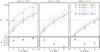 |
Fig. 1 Upper: expected mean number count in spheres (solid line, from Eq. (2)) with respect to the observed one (symbols) for the various luminosity cuts and for the three redshift bins [ 0.5,0.7 ] (left panel), [ 0.7,0.9 ] (central panel), and [ 0.9,1.1 ] (right panel). The selection in absolute magnitude MB in B-band, corresponding to each symbols/lines and colors, are indicated in the inset. The dotted line displays the |

The data set used in this paper and the other papers of this early science release is the VIPERS Public Data Release 1 (PDR-1) catalogue, which has been made publicly available in September 2013. This includes 55 359 objects, spread over a global area of 8.6 × 1.0 deg2 and 5.3 × 1.5 deg2 in W1 and W4, respectively. This corresponds to the data frozen in the VIPERS database at the end of the 2011/2012 observing campaign, i.e. 64% of the final expected survey. For the specific analysis presented here, the sample has been further limited to its higher-redshift part, selecting only galaxies with 0.55 <z< 1.1. The reason for this selection is related to minimizing the shot noise and maximizing the volume. This reduces the usable sample to 18 135 and 16 879 galaxies in W1 and W4, respectively (always with quality flags between 2 and 9). The corresponding effective volume of the two samples are 6.57 and 6.14 × 10⁶h-3 Mpc3. At redshift, z = 1.1 the two volumes span the angular comoving distances ~370 and 230 h-1 Mpc, respectively. We divide the W1 and W4 fields into three redshift bins and we build magnitude limited subsamples in each of them. For convenience, we use the magnitude limits that are listed in Table 1 of di Porto et al. (2014), which we recall in Table 1.
Magnitude selected objects (in B-band) in the VIPERS PDR-1.
The VIMOS footprint has an important impact on the observed probability of finding N galaxies in a randomly placed spherical cell in the survey volume. As a matter of fact, a direct appreciation of the masked area can be shown on the first moment of the probability distribution, i.e. the expectation value of the number count  . On the one hand, we can predict the mean number of objects per cells from the knowledge of the number density in each considered redshift bins and, on the other hand, we can estimate it by placing a regular grid of spherical cells of radius R into the volume surveyed by VIPERS. In fact, given the solid angle of W1 and W4 and the corresponding number of galaxies N1 and N4 contained in a redshift bin that has been extracted from each field, we can estimate the total number density as
  (1)where Vk is defined as the volume corresponding to a sector of a spherical shell with a solid angle equal to unity. In the case of VIPERS PDR-1, the effective solid angles that correspond to W1 and W4 are Ω1 = 1.6651683 × 10⁻³ and Ω4 = 1.5573021 × 10⁻³ (in square radians), respectively. The corresponding expected number of objects in each cell can be predicted by multiplying the averaged number density by the volume of a cell. This reads as
  (2)in the case of the spherical cells of radius R, as considered in this work. The expectation value
  , with respect to the radius of the cells corresponding to each luminosity sub-sample extracted from VIPERS-PDR1, is represented by lines in Fig. 1. In the same figure, we display the measured mean number of object
  in each redshift bins. We note that, to perform this measurement, we place a grid of equally separated (4 h-1 Mpc) spheres of radius R = 4,6,8 h-1 Mpc and we reject spheres with more than 40% of their volume outside the observed region (see Bel et al. 2014). We quantify the effect of the mask using the quantity
  (3)In fact the bottom panels of Fig. 1 show that, for all subsamples and at all redshifts, the neat effect of the masks is to under-sample the galaxy field by roughly 72%. It also shows that the correction factor α depends on the redshift that is considered, on the luminosity, and on the cell-size. The scale dependency can be explained by the fact that the correction parameter α depends on how the cells overlap with the masked regions. The left panel of Fig. 1 suggests that, at low redshift, the mask effect behaves in the same way for all the luminosity samples, while the middle panel shows a clear dependency with respect to luminosity. The correction factor α depends on the redshift distribution. As a result, the apparent dependency with respect to the luminosity is due to the dependence of the number density with respect to the luminosity of the considered objects.
The mask not only modifies the mean number of object, it also modifies the higher order moments of the distribution in such a way that the measured PN will be systematically altered. In this paper, we show that this systematic effect can be taken into account by measuring the underlying probability density function of the galaxy density contrast δ. It has been shown (see Fig. 8 of Bel et al. 2014) that, after rejecting spheres with more than 40% of their volume outside the survey, the local poisson process approximation holds. The same kind of rejection criteria is implemented by Cappi et al. (2015) to measure the moments of the galaxy distribution function. In our case, it allows us to use the ‘wrong’ probability distribution function to get reliable information on the underlying probability density function p(δ). By then applying the Poisson sampling, we can recover the unaltered PN using that  . For the sake of completeness, we provide tthe measured probability function that was obtained after rejecting the cells with more than 40% of their volume outside the survey (see Fig. 8).
In particular, let PM and PN, respectively, be the observed and the true counting probability distribution function (CPDF). Assuming that, from the knowledge of PM, there exists a process to get the underlying probability density function of the stochastic field Λ, which is associated with the random variable N, one can compute the true CPDF applying ![Mathematical equation: \begin{equation} P_N=\int_0^\infty P[N|\Lambda]p(\Lambda)\dif\Lambda, \label{sampling} \end{equation}](/articles/aa/full_html/2016/04/aa26455-15/aa26455-15-eq94.png) (4)where P [ N | Λ ] is called the sampling conditional probability; this determines the sampling process from which the discrete cell-count arises. In the following, we assume that this sampling conditional probability follows a Poisson law (Layzer 1956), and as a result in Eq. (4) we substitute
(4)where P [ N | Λ ] is called the sampling conditional probability; this determines the sampling process from which the discrete cell-count arises. In the following, we assume that this sampling conditional probability follows a Poisson law (Layzer 1956), and as a result in Eq. (4) we substitute ![Mathematical equation: \begin{equation} P[N|\Lambda]=K[N, \Lambda]\equiv \frac{\Lambda^N}{N!}{\rm e}^{-\Lambda}. \label{pkernel} \end{equation}](/articles/aa/full_html/2016/04/aa26455-15/aa26455-15-eq96.png) (5)It is also convenient to express Eq. (4) in terms of the density contrast of the stochastic field Λ,
(5)It is also convenient to express Eq. (4) in terms of the density contrast of the stochastic field Λ,  , it follows that
 ![Mathematical equation: \begin{equation} P_N=\int_{-1}^\infty K[N|\bar N(1+\delta)]p(\delta)\dif\delta, \label{samplingd} \end{equation}](/articles/aa/full_html/2016/04/aa26455-15/aa26455-15-eq98.png) (6)where we used
(6)where we used  , which is a property of the Poisson sampling.
Continuing in this direction, we propose to compare three methods which aim at extracting the underlying probability density function (PDF) to correct the observed CPDF from the angular selection effects of VIPERS.
3. Methods
In this section we review the PDF estimators that we use and compare them with each other in this paper. The purpose is to select the method that is more adapted to the characteristics of VIPERS.
3.1. The Richardson-Lucy deconvolution
This is an iterative method that aims at inverting Eq. (6) without parametrising the underlying PDF, and it has been investigated by Szapudi & Pan (2004). This method starts with an initial guess p0 for the probability density function p, which is used to compute the corresponding expected observed PN,0 via ![Mathematical equation: \begin{eqnarray*} P_{N,0}=\int_{-1}^{\infty} \hat K\left[ N, \bar N(1+\delta)\right]p_0(\delta)\dif\delta, \end{eqnarray*}](/articles/aa/full_html/2016/04/aa26455-15/aa26455-15-eq103.png) where
where ![Mathematical equation: \hbox{$\hat K\left[ N, \bar N(1+\delta)\right]\equiv K/\sum_N K$}](/articles/aa/full_html/2016/04/aa26455-15/aa26455-15-eq104.png) . The probability density function used at the next step is obtained using
. The probability density function used at the next step is obtained using ![Mathematical equation: \begin{eqnarray*} \hat p_{i+1}(\delta)=\hat p_{i}(\delta) \sum_{N=0}^{N_{\max}}\frac{P_N}{P_{N,i}} \hat K\left[ N, \bar N(1+\delta)\right], \end{eqnarray*}](/articles/aa/full_html/2016/04/aa26455-15/aa26455-15-eq105.png) where
where  . For each step, the agreement between the expected observed probability distribution PN,i and the true PN is quantified by
  It is therefore possible to know the evolution of the cost function χ2 with respect to the steps i.
In fact it has been shown by Szapudi & Pan (2004) that the cost function converges toward a constant value that corresponds with the best evaluation of the probability density function p, given the observed probability distribution PN. Since these authors have shown that this convergence occurs after around 30 iterations, we did our own convergence tests, which show that adopting a value of 30 iterations is enough. However, the evolution of the χ2 is not always monotonic. In practice, we store the χ2 result of each step and we look for the step for which the χ2 is minimum, i.e. p(δ) = pimin(δ). As an initial guess, we make sure that the discret CPDF is equal to the continuous one (p0(δ) = p).
3.2. The skewed log-normal distribution
This is a parametric method where the shape of the probability density depends on a given number of parameters, in this case the probability density function is assumed to be well described by a skewed log-normal (SLN; Colombi 1994) distribution. It is derived from the log-normal distribution (Coles & Jones 1991; Kim & Strauss 1998) but is more flexible. It is, in fact, built upon an Edgeworth expansion; if the stochastic field Φ ≡ ln(1 + δ), is following a normal distribution then the density contrast δ instead follows a log-normal distribution. In the case of the SLN density function, the field Φ follows an Edgeworth expanded normal distribution 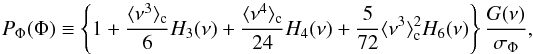 (7)where
  , G is the central reduced normal distribution
  , and ⟨ νn ⟩ c denotes the cumulant expectation value of ν. As a result, the SLN is parameterised by the four parameters μΦ, σΦ, ⟨ ν3 ⟩ c, and ⟨ ν4 ⟩ c which are related, respectively to the mean, the dispersion, the skewness, and the kurtosis of the stochastic variable Φ. They can all be expressed in terms of cumulants ⟨ Φn ⟩ c of order n of the weakly non-Gaussian field Φ. In Szapudi & Pan (2004), they use a best-fit approach and determine these parameters by minimizing the difference between the measured counting probability PN and the one obtained from
 ![Mathematical equation: \begin{eqnarray} P_N^{\rm th}&= & \int_{-1}^{\infty}K\left[N, \bar N(1+\delta)\right] P_\Phi\left[\ln(1+\delta), \mu_\Phi, \sigma_\Phi^2, \langle\Phi^3\rangle_{\rm c},\langle\Phi^4\rangle_{\rm c}\right] \nonumber \\ & &\times \dif\ln(1+\delta). \label{pth} \end{eqnarray}](/articles/aa/full_html/2016/04/aa26455-15/aa26455-15-eq128.png) (8)However, this requires us to perform the integral (Eq. (8)) in a four-dimensional parameter space which is numerically expensive.
(8)However, this requires us to perform the integral (Eq. (8)) in a four-dimensional parameter space which is numerically expensive.
In this paper, we use an alternative implementation, which is computationally more efficient. Instead of trying to maximize the likelihood of the model given the observations, we instead use the observations to predict the parameters of the SLN. To do so, we use the property of the local Poisson sampling (Bel & Marinoni 2012); the factorial moments  of the discrete counts are equal to the moments of the underlying continuous distribution ⟨ Λn ⟩. Since the transformation between the density contrast δ and the Edgeworth expanded field Φ is local and deterministic, it is possible to find a relation between the moments ⟨ Λn ⟩ and the cumulants ⟨ Φn ⟩ c.
By definition, the moments of the positive continuous field Λ are given by  Since, for a local deterministic transformation the conservation of probability imposes P(Λ)dΛ = PΦ(Φ)dΦ, it follows that the moments of Λ can be recast in terms of Φ;
 On the right hand side, we recognise the definition of the moment that generates function ℳΦ(t) ≡ ⟨ etΦ ⟩ , we therefore obtain that
  (9)This equation allows us to link the moment of Λ to the cumulants of Φ via the moment generating function ℳΦ.
Moreover, since the probability density Pφ is the product of a sum of Hermite polynomials with a Gaussian function, it is straightforward to compute the explicit expression of the moment-generating function so that we obtain 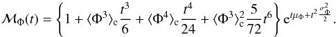 (10)In fact, Eqs. (10) and (9) together allow us to set up a system of four equations, so that for n = 1,2,3,4 it reads
  (11)where
  , X ≡ eμΦ and Bn ≡ ℳΦ(t = n,μΦ = 0,σΦ = 0). In the system of equations (Eq. (11)), the right hand side is given by observations and the left hand side depends on the cumulants μΦ,
  ,
,  , and
, and  parameterised in terms of X, Y,
  and
and  . In Appendix A, we detail the procedure to solve this non-linear system of equations. We therefore get the values of the four parameters of the SLN by simply measuring the moments of the counting variable N up to the fourth order.
3.3. The Gamma expansion
The Gamma expansion method follows the same idea as described in Sect. 3.2 but uses a Gamma distribution instead of a Gaussian one. Thit uses the orthogonality properties of the Laguerre polynomialsto modify the moments of the Gamma PDF. This type of an expansion has been investigated in Gaztañaga, Fosalba & Elizalde (2000) where they compared it to the Edgeworth expansion to model the one-point PDF of the matter-density field. Since then it has been extended further by Mustapha & Dimitrakopoulos (2010), in a more general context, to multi-point distributions.
As mentioned above the Gamma expansion requires the use of the Gamma distribution φG defined as  (12)where Γ is the Gamma function (for an integer n, Γ(n + 1) = n !, θ and k are two parameters, which are related to the first two moments of the PDF. If the galaxy probability density function is well described by a Gamma expansion at order n then it can be formally written as
  (13)where, by definition,
  ,
,  ,
,  . The function
  represents the expansion. which aims at tuning the moments of the Gamma distribution; we note that the exponent (k − 1) is not the derivative of order k − 1. Since this expansion is built upon the orthogonal properties of products of Laguerre polynomials with the Gamma distribution, the function is given by the sum
 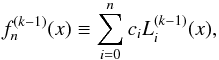 (14)where
  are the generalised Laguerre polynomials of order i and the coefficients ci represent the coefficients of the Gamma expansion and therefore depend on the moments of the galaxy field Λ:
 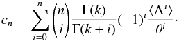 (15)The main interrest of the Gamma expansion with respect to the SLN is that the coefficients of the expansion are directly related to the moments of the distribution we want to model, i.e. it is not necessary to solve a complicated non-linear system of equations, or perform a likelihood estimation of the coefficients. Moreover, it can be easily performed at higher order to describe, as well as possible, the underlying probability-density function of galaxies.
Another advantage of describing the galaxy field Λ by a Gamma expansion probability-density function is that the corresponding observed PN can be expressed analytically, which is not the case for the SLN, which must be integrated numerically.
In Appendix B we demonstrate the previous statement, which follows that the CPDF PN can be calculated from 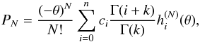 (16)where
  and, in this case, we use the notation
  . The successive derivatives of hi can be obtained from the recursive relation
 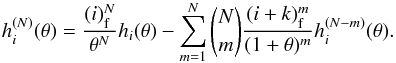 In addition to the fact that having the possibility of computing the corresponding observed PN without requiring an infinite integral for each number N is computationally more efficient, it is also practical to have the analytical calculation for some particular values of the k parameter of the distribution. In fact, when k is lower than 1, which occurs on small scales (4 h-1 Mpc), the probability-density function goes to infinity when Λ goes to 0 (although the distribution is still well defined). In particular, this numerical divergence would induce large numerical uncertainties in the computation of the void probability P0. Moreover, one can see that, for the void probability, we have the simple relation
 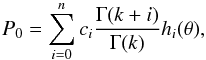 (17)which can be used to recover the true void probability in VIPERS.
4. Application of the methods on a synthetic galaxy distribution
In this section we analyse a suite of synthetic galaxy distributions generated from 20 realizations of a Gaussian stochastic field. The full process involved in generating these benchmark catalogues is detailed in Appendix C. Each comoving volume has a cubical geometry of size 500 h-1 Mpc. We generate the galaxies by discretizing the density field according to the sampling conditional probability P [ N | Λ ] , which we assume to be a Poisson distribution with mean Λ. In this way, we know the true underlying galaxy density contrast δ. We can therefore perform a reasonable comparison between the methods introduced in Sect. 3.
To avoid the effect of the grid (0.95 h-1 Mpc), we smooth both the density field and the discrete field using a spherical top-hat filter of radius R = 8 h-1 Mpc. We apply the three methods mentioned in Sect. 3 and compare the reconstructed probability-density function to the one expected to be obtained directly from the density field δ.
The discrete distribution of points contains an average number of object per cell  which is the one that is expected, according to our sampling process. The corresponding PN is given by the black histogram in the lower panel of Fig. 2. From this measurement we apply the three methods R-L, SLN, and Γe and obtain an estimation of the probability density function that corresponds to each method. In the upper panel of Fig. 2, we compare the performance of the three methods at recovering the true probability-density function (the black histogram referred to as a reference in the inset). We note that, for this test case, we use a Gamma expansion at order 4 to be coherent with the order of the expansion of the skewed log-normal. We have also represented the probability-density function, estimated when neglecting the shot noise (red dotted line), which is used as the initial guess in the case of the R-L method.
From the top panel of Fig. 2, we can conclude that the three methods perform reasonably well. It seems that the Γe method reproduces the density distribution of under-dense regions (δ ~ − 1) better but this is expected in the sense that the distribution used to generate the synthetic catalogues is a Gamma distribution (see Appendix C). However, this is not obvious because the scale on which the density field has been set up is one order of magnitude smaller than the scale of the reconstruction R = 8 h-1 Mpc.
The performance of the three methods is also represented in the bottom panel of Fig. 2, in which we compare the expected observed PN we compare the PN that is expected from the underlying density distribution obtained from each method to the true probability distribution. It can be seen that they all agree at the 15% level, hence it is not possible to conclude that one is better than an other. This scenario was actually expected, based on a comparison of the underlying density field (Fig. 2). Indeed, if one of the methods did not agree with the PDF, then we would also expect a disagreement on the observed CPDF (see Sect. 6).
Below, we investigate the sensitivity of the three methods with respect to the shot noise. In fact, as shown in Fig. 1, we will work with a high shot noise level ( ) in most of the sub-samples of VIPERS PDR-1. We therefore randomly under-sample the fake galaxy distribution by keeping only 10% of the total number of objects contained in each comoving volume. This process gives an average number per cell of 0.8, which is more representative in the context of the application of the reconstruction method. We perform the same comparison as in the ideal case (
 ) and find that the R-L method appears to be highly sensitive to shot noise. In fact, if the mean number of objects per cell is too few then the output of the method depends too much on the initial guess. It follows that, if it is too far from the true PDF, the process does not converge (see top panel of Fig. 3) and the corresponding PN does not match the observed PN (see bottom panel of Fig. 3). We note that we explicitly checked this effect by increasing the number of iterations from 30 to 200. While in the case of both the SLN and the Gamma expansion, in Fig. 3 we can see the output probability-density function is in agreement (with a larger scatter) to the one obtained in the case. This means that the sensitivity regarding to the shot noise is much smaller when considering parametric methods.
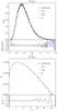 |
Fig. 2 Upper: black histogram with error bars showing the true underlying probability-density function (referred to as reference in the inset) compared to the reconstruction obtained with the R-L (red dashed line), the SLN (green dot-dashed line), and the Γe (blue long dashed line) methods. The red dotted histogram shows the PDF used as the initial guess for the R-L method and the coloured dotted lines around each method line represent the dispersion of the reconstruction among the 20 fake galaxy catalogues. We also display the relative difference of the result obtained from each method with respect to the true PDF. Lower: the black histogram with error bars shows the observed probability-density function (referred to as reference in the inset) compared to the reconstruction obtained with the R-L (red dashed line), the SLN (green dot-dashed line), and the Γe (blue long dashed line) methods. We also display the relative difference in the result obtained from each method with respect to the observed PN. |
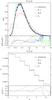 |
Fig. 3 Same as in Fig. 2, but we use only 10% of the galaxies contained in the fake galaxy catalogues. As a result, the average number of galaxies per cell drops from |


Considering the sensitivity of the R-L method to the initial guess, knowing that the average number of galaxies per cell can be lower than unity and, finally, taking computational time into account, we continue our analysis using only the two parametric methods SLN and Γe. In the following, we compare them using more realistic mock catalogues for which we don’t know, apriori, the true underlying PDF.
5. Performances in realistic conditions
In this section, we discuss how observational effects have been accounted for in our analysis and test the robustness of the reconstruction methods SLN and Gamma expansion. For this purpose we use a suite of mock catalogues created from the Millenium simulation, which are also used in the analysis performed by di Porto et al. (2014).
We compare the reconstruction methods between two catalogues, namely REFERENCE and MOCK. The reference is a galaxy catalogue that was obtained from semi-analytical models. We simulate the redshift errors of VIPERS PDR-1 by perturbing the redshift (including distortions owing to peculiar motions) with a normally distributed error with rms 0.00047(1 + z). Each MOCK catalogue is built from the corresponding REFERENCE catalogue by applying the same observational strategy (de la Torre et al. 2013) which is applied to VIPERS PDR-1; spectroscopic targets are selected from the REFERENCE catalogue by applying the slit-positioning algorithm (SPOC, Bottini et al. 2005) with the same settings as for the PDR-1. This allows us to reproduce the VIPERS footprint on the sky, the small-scale angular incompleteness that is due to spectra collisions, and the variation of the target sampling rate across the fields. Finally, we deplete each quadrant to reproduce the effect of the survey success rate (SSR, see de la Torre et al. 2013). In this way, we end up with 50 realistic mock catalogues, which simulate the detailed survey completeness function and observational biases of VIPERS in the W1 and W4 fields.
To perform a similar analysis to the one we aim at doing for VIPERS PDR-1, we construct subsamples of galaxies selected according to their absolute magnitude MB in B-band; we take all objects brighter than a given luminosity. We list these samples in Table 2, having a total of six galaxy samples. The highest luminosity cut (MB − 5log (h) < 19.72 − z) allows us to follow a single population of galaxies at three cosmic epochs.
List of the magnitude selected objects (in B-band) in the mock catalogues.
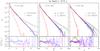 |
Fig. 4 Comparison between the SLN and Γe methods at 0.9 <z< 1.1. Each panel corresponds to a cell radius R of 4, 6, and 8 h-1 Mpc from left to right. Top: the red histogram shows the observed PDF in the MOCK catalogues while the black histogram displays the PDF extracted from the REFERENCE catalogues. The blue diamonds with lines and the magenta triangles each show the Γe expansion performed in the REFERENCE and MOCK catalogues, respectively. On the other hand, the cyan diamonds with lines and the orange triangles show, respectively, the SLN expansion performed in the REFERENCE and MOCK catalogues. Bottom: relative deviation of the Γe and SLN expansions applied to both the REFERENCE and MOCK catalogues with respect to the PDF of the REFERENCE catalogues. |
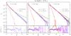 |
Fig. 5 Comparison between the SLN and Γe methods at 0.7 <z< 0.9. Each panel corresponds to a cell radius R of 4, 6, and 8 h-1 Mpc from left to right. |
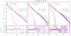 |
Fig. 6 Comparison between the SLN and Γe methods at 0.5 <z< 0.7. Each panel corresponds to a cell radius R of 4, 6, and 8 h-1 Mpc from left to right. |
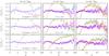 |
Fig. 7 Comparison between the SLN and Γe methods. Each column corresponds to a cell radius R of 4, 6, and 8 h-1 Mpc from left to right, and each row corresponds to a combination of redshift and magnitude cut. |
In Figs. 4–6, we show the reconstruction performances for the SLN and the Γe method. We consider the same population (Mb − 5log h + z< −19.72) but in three redshift bins, 0.9 <z< 1.1, 0.7 <z< 0.9, and 0.5 <z< 0.7. To test the stability of the methods, we perform the reconstruction using three smoothing scales, R = 4, 6, and 8 h-1 Mpc. The comparison is done as follows, on the one hand we estimate the true PN from the REFERENCE catalogue (before applying the observational selection) and we perform the reconstruction on it so that we can test the intrinsic biases that are the result of the assumed parametric method (SLN or Γe). On the other hand, we estimate the observed PM in the MOCK catalogues, from which we perform the reconstruction to verify if we recover the expected PN from the REFERENCE catalogue.
Looking more closely at Fig. 4, firstly, we can see that the intrinsic error that is due to the specific modelling of the methods is much greater for the SLN (cyan diamonds compared to the black histogram) than for the Γe (magenta diamonds compared to the black histogram). From the top panel we see that the SLN does not reproduce the tail of the CPDF, and from the bottom panel we see that, even for low counts, it shows deviations as large as 20%. This intrinsic limitation propagates when performing the reconstruction on the MOCK catalogue (orange triangles compared to the black histogram) while, for the Γe, we see that the agreement is better than 10% (magenta triangles compared to the black histogram) in the low count regime and the tail is fairly well reproduced. In the second place, comparing the Γe that was performed on the REFERENCE and the MOCK catalogues (blue diamonds with respect to magenta triangles), we can see the loss of information owing to the observational strategy that has, at most, an impact of 10% on the reconstructed CPDF, which is reduced when considering larger cells (less shot noise).
In general, Figs. 5 and 6 confirm that for the considered galaxy population the same results hold at lower redshifts. However, the reconstruction at R = 4 h-1 Mpc can, in particular, exhibit deviations larger than 20%, which is at odds with the fact that the shot noise contribution is expected to be the same for the three redshift bins (magnitude limited). We attribute this larger instability to the fact that, not only is the shot noise contribution higher for R = 4 h-1 Mpc, but the volume probed is also smaller when decreasing the redshift.
The performances of the reconstruction for the last three galaxy samples are shown in Fig. 7, where each row corresponds to a galaxy sample (we only show the residual with respect to the REFERENCE). This comparison allows us to claim that the reconstruction instability at 4 h-1 Mpc was indeed due to the high level of shot noise. We can conclude that, in the HOD galaxy mock catalogues, the galaxy distribution is more likely to be modelled by a Γe instead of an SLN. Finally, for a chosen reconstruction method, the information contained in the MOCK catalogues is enough to be able to reconstruct the CPDF of the REFERENCE catalogue at the 10% level.
6. VIPERS PDR-1 data
In this section, we apply the reconstruction method to the VIPERS PDR-1. In the previous sections, we saw that the SLN and Γe methods are sensitive to the assumptions we make about the underlying PDF. In fact, we saw in Sect. 4 that, if the underlying PDF is close to the chosen model, then the reconstruction works. In Sect. 5, we found that the galaxy distribution arising from semi-analytic models is better described by a Γe than an SLN distribution. However, in the following we do not take for granted that the same property holds for galaxies in the PDR-1.
We want to choose which one of the two distributions (log-normal or gamma) best describes the observed galaxy distribution in VIPERS PDR-1, when no expansion is applied. Thus, we compare the observed PDF to the one that is expected from the Poisson sampling of the log-normal probability density function (PS-LN) and to the one that is expected from the Poisson sampling of the Gamma distribution (the so-called negative binomial). Error bars are obtained by performing a jack-knife resampling of 3 × 7 subregions in each of the fields, W1 and W4.
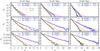 |
Fig. 8 Observed count-in-cell probability distribution function PN (histograms) from VIPERS PDR-1 for various luminosity cuts (indicated in the inset). Each row corresponds to a redshift bin, from the bottom to the top, 0.5 <z< 0.7, 0.7 <z< 0.9, and 0.9 <z< 1.1. Each column corresponds to a cell radius R = 4,6,8 h-1 Mpc from left to right. Moreover we added the expected PDF from two models which match the two first moments of the observed distribution; the red solid line shows the prediction for a Poisson-sampled log-normal (PS-LN) CPDF, while the green dashed line indicates the negative binomial model for the CPDF. |
The SP-LN distribution does not have an analytic expression and must be obtained by numerically integrating Eq. (6), while the Poisson sampling of the Gamma distribution leads to the negative binomial distribution defined as  (18)where
  and
and  to ensure that the first two moments of the negative binomial match those of the observed distribution. We note that the applicability of the negative binomial to galaxies was first suggested by Carruthers & Duong-van (1983). In Fig. 8, we show the outcome of this comparison; it follows that the negative binomial is much closer to the observed PDF than the PS-LN. This is in agreement with what has been found by Yang & Saslaw (2011), who compared the negative binomial and the gravitational equilibrium distribution (Saslaw & Hamilton 1984) to model the galaxy clustering. As a result, the underlying galaxy distribution is more likely to be described by a Gamma distribution than by a log-normal. Hence, we only use the Gamma expansion to model the galaxy distribution of VIPERS PDR-1.
Moreover, the use of the Gamma expansion instead of the SLN substantially simplifies the analysis. In Fig. 9 we provide the reconstructed probability-distribution function of VIPERS PDR-1, together with the corresponding underlying probability-density function for each redshift bin and luminosity cut. Each panel of Fig. 9 shows how the choice of a particular class of tracers (selected according to their absolute magnitude in B-band) influences the PDF of galaxies. When measuring specific properties of the intrinsic galaxy distribution for each luminosity cut, it is enough to look at the CPDF. However, when comparing the distributions with each other, it is necessary to take account of the averaged number of objects per cell, which varies from sample to sample. As a result, it appears more useful to compare the properties of the different galaxy samples using their underlying probability-density function which, assuming Poisson sampling, is free from sampling-rate variation between different type of tracers.
For the two first redshift bins, we can see that the probability density function is broadening when selecting more luminous galaxies, this goes in the direction of increasing the linear bias with respect to the matter distribution. However, for the highest redshift bin, it seems that this goes in the opposite direction, despite a less significant trend. This trend might be an artifact; indeed by analysing Fig. 1, we see that, for all these samples, the averaged number of object per cell is between 0.2–0.4, which shows that theses samples could be highly affected by shot noise effects. Consequently, particular care should be taken when interpreting these three high redshift samples.
In the following, we focus on the evolution of the underlying PDF for a particular class of objects on the wide redshift range probed by VIPERS PDR-1. Figure 10 displays the outcome of this study and shows how the PDF evolves, with regard to the redshift at which it is measured, for three populations (the three highest magnitude cuts). The three populations (top, middle, and bottom panels) exhibit non-monotonic evolution in relation to the redshift. In particular, the more luminous population shows that the PDF at 0.9 <z< 1.1 appears to be systematically different to that is the two lower redshift bins. However, we see also that some instabilities appear in the reconstruction (see wiggles at high 1 + δ). This might be due to the fact that we have fewer galaxies in this sample, giving rise to a large shot-noise contribution ( ). Indeed, we verified that, for the high mass bin and the two other galaxy populations, if we vary the order of the expansion from 6 to 4, the resulting PDF changes by less than 1σ, while for the most luminous population, truncating the expansion at order 4 only removes the instability without changing the overall behaviour of the PDF significantly. This consistency test shows that the radical change in the measured PDF for the highest redshift bin appears to be the true feature. Probably only the final VIPERS data set will be able to give a robust conclusion.
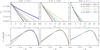 |
Fig. 9 Top: reconstructed PDF applying the Γe method in three redshift bins (from left to right) at the intermediate smoothing scale R = 6 h-1 Mpc. Bottom: underlying PDF corresponding to the CPDF in the top panel, for each luminosity cut the 1-sigma uncertainty is represented by the dotted lines. |
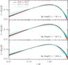 |
Fig. 10 Evolution of three galaxy populations, selected according to their luminosity (from bottom to top). On each panel, the black solid, red dashed, and cyan dot-dashed lines represent, respectively, the three redshift bins 0.5 <z< 0.7, 0.7 <z< 0.9, and, 0.9 <z< 1.1. |
Coefficients of the Γe expansion, which describe the VIPERS PDR-1 data for R = 6 h-1 Mpc.
Finally, in Table 3, we list the relevant coefficients of the Gamma expansion, which we measured from the VIPERS PDR-1 at the scale R = 6 h-1 Mpc. These can be used to model both the CPDF (Eq. (16)) and the PDF (Eq. (13)).
7. Summary
The main goal of the present paper is to measure the probability of finding N galaxies falling into a spherical cell that is randomly placed inside a sparsely sampled (i.e. with masked areas or with low-sampling rate) spectroscopic survey. Our overall approach to this problem has been to use the underlying probability-density distribution of the density contrast of galaxies to recover the counting probability that has been corrected from sparseness effects. We therefore compared three ways (R-L, SLN and Γe) of measuring the probability density of galaxies that are classified in two categories: direct and parametric. We found that, when the sampling is high ( ), the direct method (Rychardson-Lucy deconvolution) performs well and avoids putting any prior on the shape of the distribution. On the other hand, we saw that, when the sampling is low (
 ), the direct method fails to converge to the true underlying distribution. We thus concluded that, in such cases, the only alternative is to use a parametric method.
We presented two parametric forms that are aimed at describing the galaxy density distribution, the SLN, which is often used in the literature to model the matter distribution and the Γe. Despite the fact that the two distributions used in this paper already have been investigated in previous works, the approach we propose to estimate their parameters is completely new. Previously, fitting procedures were used to estimate parameters. Here we propose to measure the parameters of the distributions directly from the observations. The method can be applied to both SLN and Γe distributions and decreases the computational time of the process considerably.
Relying on simulated galaxy catalogues of VIPERS PDR1, we tested the reconstruction scheme of the counting probability (PN) under realistic conditions in the case of the SLN and Γe expansions. We found, that the reconstruction depends on the choice of the model for the galaxy distribution. However, we have also shown that it is possible to test which distribution better describes the observations.
Using VIPERS PDR1, on the relevant scales that are investigated in this paper (R = 4,6,8 h-1 Mpc), we found that the Γ distribution gives a better description of the observed PN than that provided by the log-normal (see Fig. 8). We therefore adopted the Γe parametric form to reconstruct the probability-density functions of galaxies. From these reconstruction we studied how their PDF changes according to their absolute luminosity in B-band and we also studied their redshift evolution. We found that little evolution has been detected in the first two redshift bins, while it seems that the density distribution of the galaxy field is strongly evolving in the last redshift bin.
Finally, we used the measured PDF to reconstruct the counting probability (CPDF) that would be observed if VIPERS was not masked by gaps between the VIMOS quadrants.
Acknowledgments
J.B. acknowledges useful discussions with E. Gaztañaga. We acknowledge the crucial contribution of the ESO staff for the management of service observations. In particular, we are deeply grateful to M. Hilker for his constant help and support of this programme. Italian participation in VIPERS has been funded by INAF through PRIN 2008 and 2010 programmes. J.B., L.G. and B.J.G. acknowledge support of the European Research Council through the Darklight ERC Advanced Research Grant (# 291521). OLF acknowledges support of the European Research Council through the EARLY ERC Advanced Research Grant (# 268107). A.P., K.M., and J.K. have been supported by the National Science Centre (Grants UMO-2012/07/B/ST9/04425 and UMO-2013/09/D/ST9/04030), the Polish-Swiss Astro Project (co-financed by a grant from Switzerland, through the Swiss Contribution to the enlarged European Union), the European Associated Laboratory Astrophysics Poland-France HECOLS and a Japan Society for the Promotion of Science (JSPS) Postdoctoral Fellowship for Foreign Researchers (P11802). G.D.L. acknowledges financial support from the European Research Council under the European Community’s Seventh Framework Programme (FP7/2007-2013)/ERC grant agreement no. 202781. W.J.P. and R.T. acknowledge financial support from the European Research Council under the European Community’s Seventh Framework Programme (FP7/2007-2013)/ERC grant agreement no. 202686. W.J.P. is also grateful for support from the UK Science and Technology Facilities Council through Grant ST/I001204/1. E.B., F.M. and L.M. acknowledge the support from grants ASI-INAF I/023/12/0 and PRIN MIUR 2010-2011. C.M. is grateful for support from specific project funding of the Institut Universitaire de France and the LABEX OCEVU.
References
- Bel, J., & Marinoni, C. 2012, MNRAS, 424, 971 [NASA ADS] [CrossRef] [Google Scholar]
- Bel, J., Marinoni, C., Granett, B. R., et al. (the VIPERS Team) 2014, A&A, 563, A37 [NASA ADS] [CrossRef] [EDP Sciences] [Google Scholar]
- Bernardeau, F., Colombi, S., Gaztaãga, E., & Scoccimarro, R. 2002, Phys. Rep., 367, 1 [NASA ADS] [CrossRef] [EDP Sciences] [MathSciNet] [Google Scholar]
- Bottini, D., Garilli, B., Maccagni, D., et al. 2005, PASP, 117, 996 [NASA ADS] [CrossRef] [Google Scholar]
- Bouchet, F. R., Strauss, M. A., Davis, M., et al. 1993, ApJ, 417, 36 [NASA ADS] [CrossRef] [Google Scholar]
- Cappi, A., Marulli, F., Bel, J., et al. (the VIPERS team) 2015, A&A, 579, A70 [NASA ADS] [CrossRef] [EDP Sciences] [Google Scholar]
- Carruthers, P., Duong-van, M. 1983, Phys. Lett. B, 131, 116 [NASA ADS] [CrossRef] [Google Scholar]
- Coles, P., & Jones, B. 1991, MNRAS, 248, 1 [NASA ADS] [CrossRef] [Google Scholar]
- Colless, M., Dalton, G., Maddox, S., et al. 2001, MNRAS, 328, 1039 [NASA ADS] [CrossRef] [Google Scholar]
- Colombi, S. 1994, ApJ, 435, 536 [NASA ADS] [CrossRef] [Google Scholar]
- de la Torre, S., Guzzo, L., Kovac, K., et al. (the ZCOSMOS collaboration) 2010, MNRAS, 409, 867 [NASA ADS] [CrossRef] [Google Scholar]
- de la Torre, S., Guzzo, L., Peacock, J. A., et al. (VIPERS team) 2013, A&A, 557, A54 [NASA ADS] [CrossRef] [EDP Sciences] [Google Scholar]
- di Porto, C., Branchini, E., Bel, J., et al. (VIPERS team) 2014, A&A, submitted [arXiv:1406.6692] [Google Scholar]
- Eisenstein, D. J., & Hu, W. 1998, ApJ, 496, 605 [NASA ADS] [CrossRef] [Google Scholar]
- Garilli, B., Le Fèvre, O., Guzzo, L., et al. (the VVDS collaboration) 2008, A&A, 486, 683 [NASA ADS] [CrossRef] [EDP Sciences] [Google Scholar]
- Garilli, B., Paioro, L., Scodeggio, M., et al. 2012, PASP, 124, 1232 [NASA ADS] [CrossRef] [Google Scholar]
- Garilli, B., Guzzo, L., Scodeggio, M., et al. (the VIPERS team) 2014, A&A, 562, A23 [NASA ADS] [CrossRef] [EDP Sciences] [Google Scholar]
- Gaztañaga, E., Fosalba, P., & Elizalde, E. 2000, ApJ, 539, 522 [NASA ADS] [CrossRef] [Google Scholar]
- Greiner, M., & Enβlin, T. A. 2015, A&A, 574, A86 [NASA ADS] [CrossRef] [EDP Sciences] [Google Scholar]
- Guzzo, L., Pierleoni, M., Meneux, B., et al. (the VVDS team) 2008, Nature, 451, 541 [NASA ADS] [CrossRef] [PubMed] [Google Scholar]
- Guzzo, L., Scodeggio, M., Garilli, B., et al. (the VIPERS team) 2014, A&A, 566, A108 [NASA ADS] [CrossRef] [EDP Sciences] [Google Scholar]
- Kim, R. S. J., & Strauss, M. A. 1998, ApJ, 493, 39 [NASA ADS] [CrossRef] [Google Scholar]
- Layzer, D. 1956, AJ, 61, 383 [NASA ADS] [CrossRef] [Google Scholar]
- LeFèvre, O., Saisse, M., Mancini, D., et al. 2003, Proc. SPIE, 4841, 1670 [NASA ADS] [CrossRef] [Google Scholar]
- Le Fèvre, O., Vettolani, G., Garilli, B., et al. 2005, A&A, 439, 845 [NASA ADS] [CrossRef] [EDP Sciences] [Google Scholar]
- Lilly, S. J., Le Brun, V., Maier, C., et al. (the ZCOSMOS collaboration) 2009, ApJS, 184, 218 [Google Scholar]
- Marchetti, A., Granett, B. R., Guzzo, L., et al. (the VIPERS team) 2013, MNRAS, 428, 1424 [NASA ADS] [CrossRef] [Google Scholar]
- Mellier, Y., Bertin, E., Hudelot, P., et al. 2008, The CFHTLS T0005 Release, http://terapix.iap.fr/cplt/oldSite/Descart/CFHTLS-T0005-Release.pdf [Google Scholar]
- Mustapha, H., & Dimitrakopoulos, R. 2010, Int. Conf. of Numerical Analysis and Appl. Math., AIP Conf. Proc., 60, 2178 [Google Scholar]
- Newman, J. A., Cooper, M. C., Davis, M., et al. (the DEEP2 collaboration) 2013, ApJS, 208, 5 [Google Scholar]
- Oke, J. B., & Gunn, J. E. 1983, ApJ, 266, 713 [NASA ADS] [CrossRef] [Google Scholar]
- Saslaw, W. C., & Hamilton, A. J. S. 1984, ApJ, 276, 13 [NASA ADS] [CrossRef] [Google Scholar]
- Scodeggio, M., Franzetti, P., Garilli, B., et al. 2009, The Messenger, 135, 13 [NASA ADS] [Google Scholar]
- Szapudi, I., & Pan, J. 2004, ApJ, 602, 26 [NASA ADS] [CrossRef] [Google Scholar]
- Szapudi, I., Meiksin, A., Nichol, R. C., et al. 1996, ApJ, 473, 15 [NASA ADS] [CrossRef] [Google Scholar]
- Yang, A., & Saslaw, W. C. 2011, ApJ, 729, 123 [NASA ADS] [CrossRef] [Google Scholar]
Appendix A: Non-linear system
The problem with this system of equations is that it is non-linear, and is therefore difficult to solve. However, it can be reduced to a one-dimensional equation which can be solved numerically.
The two first equations (n = 1 and n = 2) can be used to express the first two cumulants with respect to the third and fourth order ones: ![Mathematical equation: \appendix \setcounter{section}{1} \begin{eqnarray} \sigma_\Phi^2 & = & \ln(A_2) + \ln\left( \frac{B_1^2}{B_2}\right) \label{sig} \\ \mu_\Phi & = & -\frac{1}{2}\left [\ln(A_2) + \ln\left( \frac{B_1^4}{B_2}\right) \right ] \label{mu} , \end{eqnarray}](/articles/aa/full_html/2016/04/aa26455-15/aa26455-15-eq236.png) where B1 and B2 are both functions of x and y. Then, using other combinations of the equation, one can express a system of two equations for x and y alone:
where B1 and B2 are both functions of x and y. Then, using other combinations of the equation, one can express a system of two equations for x and y alone: 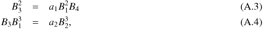 where
where  and
and  . To properly solve the system, we prefer to express it in terms of one parameter η ≡ B2/B1, moreover one can see that polynomials B1 to B4 are not independent, as a result.
  where
where  and which can be substituted in Eq. (A.3). Combining Eqs. (A.3) and (A.4) one obtains a parametric equation for B1
 (A.5)which can be solved for each value of the parameter η and an independent parametric equation for B3
 As a result we can find a couple B1, B3 for each value of the parameter η. It follows that one can express x and y with respect to η and, given the definition of η, the possible solution x and y must satisfy the condition
 ![Mathematical equation: \appendix \setcounter{section}{1} \begin{eqnarray*} B_2[x(\eta),y(\eta)]-\eta B_1[x(\eta),y(\eta)]=0, \end{eqnarray*}](/articles/aa/full_html/2016/04/aa26455-15/aa26455-15-eq252.png) which gives the possible values of η from which one can recover x and y. Finally, from Eqs. (A.1) and (A.2) we can compute the values of σΦ and μΦ that correspond to each couple (x, y) of the solutions. This allows us to select the solution which provides a value of A5 that is closer to the observed one.
which gives the possible values of η from which one can recover x and y. Finally, from Eqs. (A.1) and (A.2) we can compute the values of σΦ and μΦ that correspond to each couple (x, y) of the solutions. This allows us to select the solution which provides a value of A5 that is closer to the observed one.
Once the values of the cumulants μΦ, , ⟨ Φ3 ⟩ c and ⟨ Φ4 ⟩ c are known from the process detailed above, we know that the moments of the corresponding  will match those of the observed up to order 4. In the end, we can check whether the SLN distribution provides a good match to data by numerically integrating the probability-density function that was convolved with the Poisson kernel K (see Eq. (5)).
Appendix B: Generating function
We show that the CPDF that was associated with a Gamma expanded PDF can be calculated analytically from an expression that depends explicitly on the coefficients ci of the Gamma expansion.
Be  the generating function associated to the probability distribution PN, it is defined as
  (B.1)In case of the Poisson sampling of a Gamma distribution, after some algebra, one can show that it can be expressed with respect to the coefficients of the Gamma expansion as
  (B.2)where γ ≡ (1 − λ)θ and
  Nevertheless, this integral can be computed using the Laguerre expansion of the exponential
 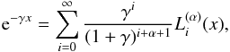 where it reads to
 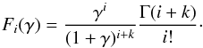 (B.3)The formal expression of the generating function is therefore given by
 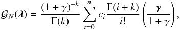 (B.4)where we still use γ = (1 − λ)θ. From the explicit expression of the moment-generating function (Eq. (B.4)) one can get the probability distribution PN by iteratively deriving the generating function with respect to γ:
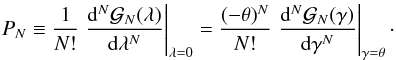 These derivatives can be calculated explicitly.
Appendix C: Synthetic galaxy catalogues
We describe here how we generate synthetic galaxy catalogues from Gaussian realizations. The first requirement of these catalogues is that they must be characterised by a known power spectrum and 1-point probability-distribution function. The second requirement is that the probability-distribution function must be measurable.
The basic idea is simple, we generate a Gaussian random field in Fourier space (assuming a power spectrum), we inverse Fourier transform it to get its analog in configuration space. We further apply a local transform to map the Gaussian field into a stochastic field that is characterised by the target PDF. The two crucial steps of this process are the choice of the input power spectrum and the choice of the local transform.
Be ν a stochastic field following a centered (⟨ ν ⟩ = 0) reduced ( ) Gaussian distribution. From a realization of this field, one can generate a non-Gaussian density field δ by applying a local mapping L between the two, hence
  (C.1)The local transform L must be chosen to match some target PDF Pδ for the density contrast δ. Assuming that the local transform is a monotonic function, which maps the ensemble ]−∞, +∞[ into ]−1, +∞[ then, owing to the probability conservation Pδ(δ)dδ = Pν(ν)dν, the local transform must verify the following matching:
 ![Mathematical equation: \appendix \setcounter{section}{3} \begin{equation} \mathcal{C}_\delta[\delta] = \mathcal{C}_\nu[\nu], \label{matching} \end{equation}](/articles/aa/full_html/2016/04/aa26455-15/aa26455-15-eq277.png) (C.2)where
(C.2)where  stands for the cumulative probability distribution function. If [ a,b ] is the definition assemble of the variable x, then its cumulative probability distribution function is defined as
 ![Mathematical equation: \hbox{$\mathcal{C}_x[x]\equiv \int_{a}^xP_x(x^\prime)\dif x^\prime$}](/articles/aa/full_html/2016/04/aa26455-15/aa26455-15-eq280.png) , where Px is the PDF of x. By definition a probability-density function is positive, it follows that its cumulative is a monotonic function and therefore Eq. (C.2) can always be inverted to read
, where Px is the PDF of x. By definition a probability-density function is positive, it follows that its cumulative is a monotonic function and therefore Eq. (C.2) can always be inverted to read ![Mathematical equation: \appendix \setcounter{section}{3} \begin{eqnarray*} \delta=\mathcal{C}_\delta^{-1}\left [ \mathcal{C}_\nu (\nu ) \right], \end{eqnarray*}](/articles/aa/full_html/2016/04/aa26455-15/aa26455-15-eq282.png) where the exponent −1 stands for the reciprocal function such that F-1[F(x)] = x. For example, by defining the local mapping L, this allows a normal distribution to transform into a log-normal distribution, which is δ = eν − 1. We note that, depending on the PDF to be matched, this inversion can require a numerical evaluation, which can be tabulated.
where the exponent −1 stands for the reciprocal function such that F-1[F(x)] = x. For example, by defining the local mapping L, this allows a normal distribution to transform into a log-normal distribution, which is δ = eν − 1. We note that, depending on the PDF to be matched, this inversion can require a numerical evaluation, which can be tabulated.
Once a local transform is chosen, we need to address the question of finding the appropriate power spectrum of the Gaussian field ν which, once locally mapped into the density field δ, will match the expected power spectrum. Following Greiner & Enβlin (2015), who considered a log-transform, we generalised their result to a generic local transformation. This mapping is not directly in Fourier space although it is in configuration. Writing the two-point moment of order two of the density field δ and assuming the probability conservation leads to 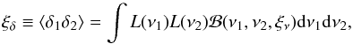 (C.3)where ℬ is a bivariate Gaussian defined as
 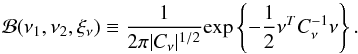 (C.4)We notice that, in our case (central reduced Gaussian), the covariance matrix Cν takes the simple form
 ![Mathematical equation: \hbox{$C_\nu = \left[ \substack{1 \,\,\, \xi_\nu \\ \xi_\nu \,\,\, 1} \right]$}](/articles/aa/full_html/2016/04/aa26455-15/aa26455-15-eq291.png) . Once integrated over the definition domain of ν1 and ν2, Eq. (C.3) provides a mapping between the two-point correlation function of the Gaussian field ν and the two-point correlation function of the density field δ. However, we prefer to rotate the coordinate system before performing the integral (C.3) because, in the case of high correlation (~1), the Gaussian will be comparable with a straight line – and most of the sampling of this function will be useless. That is why we look for the rotation that allows us to diagonalise the matrix Cν and therefore convert ν into a new variable x. It follows that
. Once integrated over the definition domain of ν1 and ν2, Eq. (C.3) provides a mapping between the two-point correlation function of the Gaussian field ν and the two-point correlation function of the density field δ. However, we prefer to rotate the coordinate system before performing the integral (C.3) because, in the case of high correlation (~1), the Gaussian will be comparable with a straight line – and most of the sampling of this function will be useless. That is why we look for the rotation that allows us to diagonalise the matrix Cν and therefore convert ν into a new variable x. It follows that ![Mathematical equation: \appendix \setcounter{section}{3} \begin{eqnarray*} C_x=\left [ \begin{array}{cc} 1 -\xi_\nu & 0\\ 0 & 1+\xi_\nu \end{array} \right] \end{eqnarray*}](/articles/aa/full_html/2016/04/aa26455-15/aa26455-15-eq296.png) and the integral becomes
and the integral becomes 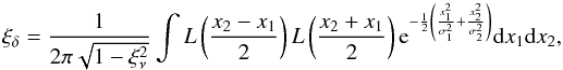 (C.5)where
  and
and  . We can therefore integrate over a bounded domain that corresponds to the −8σ1, 8σ1 along the x1 axis and −8σ2, 8σ2 along the x2 axis. Another possibility for perform the integral (C.3) is to use Mehler’s formula. By doing so, one can show that the two-point correlation of the density field can be expressed as a Taylor expansion on the two-point correlation function of the ν field. Thihs reads
 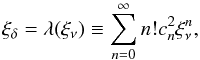 (C.6)where the cn are the coefficients of the Hermit transform of the local mapping
  . The cn coefficients can be calculated using the orthogonal properties of Hermit polynomials
  (C.7)The latter approach speeds up the numerical evaluation of Eq. (C.5) considerably. It allows us to compute the 2D integral as a finite sum of 1D integrals. It also allows us to verify that, when the two-point function of the field ν is positive, then the derivative of ξδ with respect to ξν is positive. Moreover, from Eq. (C.3) we can see that ξν = 0 implies ξδ = 0. This means that the function that transforms ξν into ξδ is invertible as long as ξδ is positive. On the other hand, we know that the zero-crossing of the two-point correlation function occurs at very large scales at which one can safely assume that | ξδ | ≪ 1. Thus, continuing along this train of thought, we can truncate Eq. (C.6) at order one, which provides a linear relation between ξδ and ξν. As a result, we can take the reciprocal of the function λ such that ξν = λ-1(ξδ).
Once the local transform L and the two-point correlation mapping λ are known, then the input power spectrum of the Gaussian field ν can be obtained as follows. We choose a power spectrum P(k), in the present case Eisenstein & Hu (1998), for the density field δ. We calculate its corresponding 2-point correlation function  (C.8)At each scale r, we can deduce the two-point correlation function of the Gaussian field ξν = λ-1(ξδ) and finally, using a Fourier transform, we obtain the input power spectrum
  (C.9)Finally, to make sure that the PDF target will be reproduced, we need to verify that its integral is indeed equal to the expected variance in the size of the mesh, once the input power spectrum Pin(k) has been set up on a regular k-space grid, which will be used to generate the Gaussian field. Thus,
  should be equal to
  . In general, σa and
  are not equal, in which case we renormalise the target power spectrum by the quantity
  ,
,  .
.
We generate a Gaussian field (with a flat power spectrum) on a regular mesh of a = 0.95 h-1 Mpc and a comoving box of 5003h-3 Mpc3. We then Fourier transform with an FFT and keep only the phases of the field νk = eiθ(k). At each position kn, we generate the value of the modulus of  , where
  and ϵ is a random number with a uniform probability distribution between 0 and 1. We then inverse Fourier transform the field to get a centred reduced Gaussian field. In Fig. C.1, we show the input power spectrum of the Gaussian field ν compared to the one that was measured using a FFT, and to the one expected from the local transformation, which was applied to the ν field to generate the density field δ.
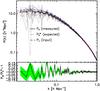 |
Fig. C.1 Upper: grey dotted lines show the power spectrum measured in each of the 20 fake galaxy distributions, the black solid line represent their average and the errors display the dispersion of the measurements. The blue long dashed line displays the input power spectrum used too generate the Gaussian stochastic field nu and the red dashed line shows the corresponding expectation value for the power spectrum of the density contrast δ. Lower: shows the deviation between the measured power spectrum of the δ-field and the expected one. |
All Tables
Coefficients of the Γe expansion, which describe the VIPERS PDR-1 data for R = 6 h-1 Mpc.
All Figures
|
Fig. 1 Upper: expected mean number count in spheres (solid line, from Eq. (2)) with respect to the observed one (symbols) for the various luminosity cuts and for the three redshift bins [ 0.5,0.7 ] (left panel), [ 0.7,0.9 ] (central panel), and [ 0.9,1.1 ] (right panel). The selection in absolute magnitude MB in B-band, corresponding to each symbols/lines and colors, are indicated in the inset. The dotted line displays the |
| In the text | |
|
Fig. 2 Upper: black histogram with error bars showing the true underlying probability-density function (referred to as reference in the inset) compared to the reconstruction obtained with the R-L (red dashed line), the SLN (green dot-dashed line), and the Γe (blue long dashed line) methods. The red dotted histogram shows the PDF used as the initial guess for the R-L method and the coloured dotted lines around each method line represent the dispersion of the reconstruction among the 20 fake galaxy catalogues. We also display the relative difference of the result obtained from each method with respect to the true PDF. Lower: the black histogram with error bars shows the observed probability-density function (referred to as reference in the inset) compared to the reconstruction obtained with the R-L (red dashed line), the SLN (green dot-dashed line), and the Γe (blue long dashed line) methods. We also display the relative difference in the result obtained from each method with respect to the observed PN. |
| In the text | |
|
Fig. 3 Same as in Fig. 2, but we use only 10% of the galaxies contained in the fake galaxy catalogues. As a result, the average number of galaxies per cell drops from |
| In the text | |
|
Fig. 4 Comparison between the SLN and Γe methods at 0.9 <z< 1.1. Each panel corresponds to a cell radius R of 4, 6, and 8 h-1 Mpc from left to right. Top: the red histogram shows the observed PDF in the MOCK catalogues while the black histogram displays the PDF extracted from the REFERENCE catalogues. The blue diamonds with lines and the magenta triangles each show the Γe expansion performed in the REFERENCE and MOCK catalogues, respectively. On the other hand, the cyan diamonds with lines and the orange triangles show, respectively, the SLN expansion performed in the REFERENCE and MOCK catalogues. Bottom: relative deviation of the Γe and SLN expansions applied to both the REFERENCE and MOCK catalogues with respect to the PDF of the REFERENCE catalogues. |
| In the text | |
|
Fig. 5 Comparison between the SLN and Γe methods at 0.7 <z< 0.9. Each panel corresponds to a cell radius R of 4, 6, and 8 h-1 Mpc from left to right. |
| In the text | |
|
Fig. 6 Comparison between the SLN and Γe methods at 0.5 <z< 0.7. Each panel corresponds to a cell radius R of 4, 6, and 8 h-1 Mpc from left to right. |
| In the text | |
|
Fig. 7 Comparison between the SLN and Γe methods. Each column corresponds to a cell radius R of 4, 6, and 8 h-1 Mpc from left to right, and each row corresponds to a combination of redshift and magnitude cut. |
| In the text | |
|
Fig. 8 Observed count-in-cell probability distribution function PN (histograms) from VIPERS PDR-1 for various luminosity cuts (indicated in the inset). Each row corresponds to a redshift bin, from the bottom to the top, 0.5 <z< 0.7, 0.7 <z< 0.9, and 0.9 <z< 1.1. Each column corresponds to a cell radius R = 4,6,8 h-1 Mpc from left to right. Moreover we added the expected PDF from two models which match the two first moments of the observed distribution; the red solid line shows the prediction for a Poisson-sampled log-normal (PS-LN) CPDF, while the green dashed line indicates the negative binomial model for the CPDF. |
| In the text | |
|
Fig. 9 Top: reconstructed PDF applying the Γe method in three redshift bins (from left to right) at the intermediate smoothing scale R = 6 h-1 Mpc. Bottom: underlying PDF corresponding to the CPDF in the top panel, for each luminosity cut the 1-sigma uncertainty is represented by the dotted lines. |
| In the text | |
|
Fig. 10 Evolution of three galaxy populations, selected according to their luminosity (from bottom to top). On each panel, the black solid, red dashed, and cyan dot-dashed lines represent, respectively, the three redshift bins 0.5 <z< 0.7, 0.7 <z< 0.9, and, 0.9 <z< 1.1. |
| In the text | |
|
Fig. C.1 Upper: grey dotted lines show the power spectrum measured in each of the 20 fake galaxy distributions, the black solid line represent their average and the errors display the dispersion of the measurements. The blue long dashed line displays the input power spectrum used too generate the Gaussian stochastic field nu and the red dashed line shows the corresponding expectation value for the power spectrum of the density contrast δ. Lower: shows the deviation between the measured power spectrum of the δ-field and the expected one. |
| In the text | |
Current usage metrics show cumulative count of Article Views (full-text article views including HTML views, PDF and ePub downloads, according to the available data) and Abstracts Views on Vision4Press platform.
Data correspond to usage on the plateform after 2015. The current usage metrics is available 48-96 hours after online publication and is updated daily on week days.
Initial download of the metrics may take a while.