The resolved star-formation relation in nearby active galactic nuclei

Viviana Casasola; Leslie Hunt; Françoise Combes; Santiago García-Burillo

doi:10.1051/0004-6361/201425313

Home

All issues

Volume 577 (May 2015)

A&A, 577 (2015) A135

Full HTML

Free Access

Issue		A&A Volume 577, May 2015


Article Number		A135
Number of page(s)		21
Section		Extragalactic astronomy
DOI		https://doi.org/10.1051/0004-6361/201425313
Published online		19 May 2015

A&A 577, A135 (2015)

The resolved star-formation relation in nearby active galactic nuclei^⋆

Viviana Casasola¹^,2, Leslie Hunt², Françoise Combes³ and Santiago García-Burillo⁴

¹ INAF−Istituto di Radioastronomia & Italian ALMA Regional Centre, via Gobetti 101, 40129 Bologna, Italy
e-mail: casasola@arcetri.astro.it
² INAF−Osservatorio Astrofisico di Arcetri, Largo E. Fermi, 5, 50125 Firenze, Italy
³ Observatoire de Paris, LERMA, CNRS UMR 8112, 61 Av. de l’Observatoire, 75014 Paris, France
⁴ Observatorio Astronómico Nacional (OAN)-Observatorio de Madrid, Alfonso XII, 3, 28014 Madrid, Spain

Received: 10 November 2014
Accepted: 25 February 2015

Abstract

Aims. We present an analysis of the relation between the star formation rate (SFR) surface density (Σ_SFR) and mass surface density of molecular gas (Σ_H₂), commonly referred to as the Kennicutt-Schmidt (K-S) relation, on its intrinsic spatial scale, i.e. the size of giant molecular clouds (~10−150 pc), in the central, high-density regions of four nearby low-luminosity active galactic nuclei (AGN). These are AGN extracted from the NUclei of GAlaxies (NUGA) survey. This study investigates the correlations and slopes of the K-S relation, as a function of spatial resolution and of the different ¹²CO emission lines used to trace Σ_H₂, and tests its validity in the high-density central regions of spiral galaxies.

Methods. We used interferometric IRAM ¹²CO(1−0) and ¹²CO(2−1) and SMA ¹²CO(3−2) emission line maps to derive Σ_H₂ and HST–Hα images to estimate Σ_SFR.

Results. Each galaxy is characterized by a distinct molecular SF relation on spatial scales between 20 to 200 pc. The K-S relations can be sublinear, but also superlinear, with slopes ranging from ~0.5 to ~1.3; slopes are generally superlinear on spatial scales >100 pc and sublinear on smaller scales. Depletion times range from ~1 and 2 Gyr, which is compatible with results for nearby normal galaxies. These findings are valid independently of which transition – ¹²CO(1−0), ¹²CO(2−1), or ¹²CO(3−2) – is used to derive Σ_H₂. Because of either star-formation feedback, the lifetime of clouds, turbulent cascade, or magnetic fields, the K-S relation might be expected to degrade on small spatial scales (<100 pc). However, we find no clear evidence of this, even on scales as small as ~20 pc, and this might be because of the higher density of GMCs in galaxy centers that have to resist higher shear forces. The proportionality between Σ_H₂ and Σ_SFR found between 10 and 100 M_⊙ pc^-2 is valid even at high densities, ~10³ M_⊙ pc^-2. However, by adopting a common CO-to-H₂ conversion factor (α_CO), the central regions of the NUGA galaxies have higher Σ_SFR for a given gas column than those expected from the models, with a behavior that lies between the mergers or high-redshift starburst systems and the more quiescent star-forming galaxies, assuming that the first ones require a lower value of α_CO.

Key words: galaxies: ISM / galaxies: spiral / galaxies: active / ISM: molecules / stars: formation

^⋆

The maps are only available at the CDS via anonymous ftp to cdsarc.u-strasbg.fr (130.79.128.5) or via http://cdsarc.u-strasbg.fr/viz-bin/qcat?J/A+A/577/A135

© ESO, 2015

1. Introduction

The relationship between gas and star formation (SF) in galaxies plays a key role in galaxy evolution. It constrains how efficiently galaxies turn their gas into stars and also serves as essential input to simulations and models (e.g., Boissier et al. 2003; Tan et al. 1999; Springel & Hernquist 2003; Krumholz & McKee 2005). Despite the importance of this relationship, the processes responsible for the conversion of gas into stars in various galactic environments are still poorly understood.

More than fifty years ago, Schmidt (1959, 1963) suggested that the star formation rate (SFR) and the gas content in galaxies are related by $\begin{matrix} Σ SFR = A Σ_{gas}^{N} \end{matrix}$ $\begin{eqnarray} \Sigma{\rm_{SFR}} = A\,\Sigma_{\rm gas}^{N} \label{eq:schmidt} \end{eqnarray}$ (1)where Σ_SFR and Σ_gas are the SFR surface density and the gas surface density, respectively, A is the normalization constant representing the efficiency of the processes regulating gas-stars conversion, and N_fit the power relation index. The gas can be atomic (Hi), molecular (H₂), or a combination of both (Hi+H₂).

Although the atomic phase of the interstellar medium (ISM) is directly traced by the Hi emission line at 21 cm, indirect approaches are needed to estimate the distribution of H₂. The molecular hydrogen indeed lacks a dipole moment and typical temperatures (15−25 K), in giant molecular clouds (GMCs) are too low to excite quadrupole or vibrational transitions. For these reasons, the carbon monoxide (CO) emission lines are the most straightforward and reliable tracer of H₂ in galaxies. CO is relatively bright and its ability to trace the bulk distribution of H₂ has been confirmed by comparisons with gamma rays (Lebrun et al. 1983; Strong et al. 1988) and dust emission (Desert et al. 1988; Dame et al. 2001). Comparing the atomic gas density with the number of representative young stellar objects in the solar neighborhood, Schmidt (1959) derived a power relation index N ≈ 2 in Eq. (1). Values of N ranging approximately from 1.5 to 2 were further confirmed by Guibert et al. (1978), using more precise data on the radial and vertical distributions of the interstellar gas and a variety of young objects as tracers of SFR.

Later, Kennicutt (1998a,b) found that for disk-averaged surface densities, both normal star-forming and starburst galaxies follow Eq. (1) with a power relation index of N ≈ 1.4 for total (Hi+H₂) gas. This correlation between gas and SFR surface density is commonly referred to as the Kennicutt-Schmidt relation (hereafter the K-S relation). Such a relation is in principle consistent with large scale gravitational instability being the major driver of dense cloud formation (Quirk 1972; Madore 1977). Although spatially unresolved studies of Hi, CO, and SFR are useful for characterizing global disk properties, understanding the mechanisms behind the SF requires resolved measurements.

It is now possible to study the K-S relation at sub-kpc scales, approaching the intrinsic scale of SF, i.e. the size of GMCs (~10−150 pc, e.g., Solomon et al. 1987). Several factors have contributed, including the explosion in multiwavelength data for nearby galaxies: for example, UV-GALEX: Gil de Paz et al. (2007); infrared-Spitzer and Hα-HST: SINGS and LVL surveys, Kennicutt et al. (2003), Dale et al. (2009); far-infrared-Herschel: KINGFISH, Kennicutt et al. (2011); ¹²CO: BIMA SONG, Helfer et al. (2003); HERACLES-IRAM 30 m, Leroy et al. (2009); Hi: VLA THINGS survey, Walter et al. (2008). Also technical improvements, especially the construction of millimeter interferometers, now allow higher resolution imaging of ¹²CO in galaxies.

There is now substantial evidence that the molecular gas is well-correlated with the SFR tracers over several orders of magnitude, but mostly for regions where H₂ makes up the majority of the neutral gas, Σ_H2 ≳ Σ_HI (e.g., Wong & Blitz 2002; Komugi et al. 2005; Kennicutt et al. 2007; Thilker et al. 2007; Schuster et al. 2007; Bigiel et al. 2008; Leroy et al. 2008; Blanc et al. 2009; Onodera et al. 2010; Verley et al. 2010; Rahman et al. 2011; Momose et al. 2013). This is because GMCs, the major reservoirs of molecular gas, are the sites of most SF in our Galaxy and other galaxies. Their properties indeed set the initial conditions for protostellar collapse and may play a role in determining the stellar initial mass function (IMF, McKee & Ostriker 2007). Moreover, it has long been known that the spatial distribution of ¹²CO emission follows that of the stellar light and Hα (e.g., Young & Scoville 1982; Scoville & Young 1983; Solomon et al. 1983; Tacconi & Young 1990). The lack of a clear correlation between Σ_HI and Σ_SFR inside galaxy disks (e.g., Bigiel et al. 2008) offers circumstantial evidence that SF remains coupled to the molecular, rather than total gas surface density (Σ_{HI + H2}) even where Hi makes up most of the ISM. Bigiel et al. (2008) find that Σ_HI saturates at surface density of ≈9 M_⊙ pc^-2, and gas in excess of this value is in the molecular phase of spirals and Hi-dominated galaxies.

A crucial parameter in the study of the resolved K-S relation is the choice of the tracer for H₂ and SFR. Most of the studies for deriving the H₂ surface density to study the molecular SF relation are based on the ¹²CO(1−0) (e.g., Rahman et al. 2011; Saintonge et al. 2011; Momose et al. 2013) or ¹²CO(2−1) emission lines (e.g., Bigiel et al. 2008; Leroy et al. 2008), and more rarely on the ¹²CO(3−2) transition (e.g., Komugi et al. 2007; Wilson et al. 2012). Also the dependence of the SFR on dense molecular gas mass has been explored with molecules such as HCN and HCO⁺ (e.g., Gao & Solomon 2004; Wu et al. 2005; García-Burillo et al. 2012).

Over the past thirty years, extensive efforts have been made to derive plausible SFRs for external galaxies (see Kennicutt 1998a; Calzetti et al. 2010, for reviews). Optical SFR tracers, such as Hα, often suffer from dust extinction, which can change dramatically from location to location. Calzetti et al. (2007) find A_V ~ 2.2 mag in typical extragalactic Hii regions and dense star-forming regions can be completely obscured with A_V that can reach ~6 mag (e.g., Scoville et al. 2001). In addition, the A_V value is not always known for a given galaxy. However, IR space facilities (Spitzer and Herschel) and UV (GALEX) have made it possible to also image the details of dust-obscured SF.

Different SFR tracers probe different time scales and hence the SF history of any particular galaxy. Hα emission traces ionized gas by massive (M> 10 M_⊙) stars on a timescale of <20 Myr. The far-UV (FUV) luminosity corresponds to relatively older (<100 Myr), less massive (≳5 M_⊙) stellar populations. The MIR 24 μm emission mostly traces reprocessed radiation of newborn (few Myr) OB stellar associations embedded within the parental molecular clouds. Although star clusters emerge from their natal clouds in less than 1 Myr, they remain associated with it on a much longer time scale, ~10−30 Myr, which is the time scale associated with the 24 μm emission as a SFR tracer. Kennicutt et al. (2007) and Calzetti et al. (2007) have justified the feasibility of correcting the number of ionizing photons, as traced by the Hα recombination line, for the effects of the dust extinction by adding a weighted component from the Spitzer MIPS 24 μm luminosity in individual star-forming regions. Leroy et al. (2008) and Bigiel et al. (2008) have proposed another composite SFR tracer that corrects dust attenuation of far-UV surface brightness using, also in this case, the Spitzer 24 μm emission but with different weights. These composite SFR tracers, Hα+24 μm and FUV+24 μm, have been extensively used for a large number of nearby galaxies (see references above).

Spatially resolved K-S relation studies published in the past decade (e.g., Kennicutt et al. 2007; Bigiel et al. 2008, 2010, 2011; Leroy et al. 2008; Blanc et al. 2009; Eales et al. 2010; Verley et al. 2010; Liu et al. 2011; Rahman et al. 2011, 2012; Schruba et al. 2011; Ford et al. 2013; Viaene et al. 2014) found a wide spread in the value of the power relation index (N ≈ 0.6−3) both within and among galaxies. For a comprehensive review of the most recent SF relation studies on sub-kpc scales, we refer to Kennicutt & Evans (2012). The wide range of the value of N may be intrinsic, suggesting that different SF “laws” exist, and may contain valuable astrophysical information. Alternatively, it may be partially or entirely due to the adopted physical scale (e.g., Schruba et al. 2010; Calzetti et al. 2012), the choice of the molecular gas (e.g., Krumholz & Thompson 2007; Narayanan et al. 2008) and SFR tracer, the type of galaxy under investigation, data sampling, and the fitting method used (e.g., Blanc et al. 2009; Shetty et al. 2013). In particular, different SFR tracers and spatial scales effectively sample different timescales, so that a galaxy’s SF history can play a role in determining the results of the measurements. It is also possible that these differences correspond to a spectrum of physical mechanisms present in a wide range of environments. High shear in galactic bars, harassment in a dense galaxy cluster, and galaxy mergers and interactions have the potential to either dampen or enhance the SF process (e.g., Casasola et al. 2004; Zhou et al. 2011; Lanz et al. 2013). All these environmental processes at work, on both galactic and extragalactic scales, suggest therefore that there is no universal SF relation in the Local Universe.

In addition to the slope of the empirical power relation relation between Σ_gas and Σ_SFR, the other crucial parameter in SF studies is the molecular gas depletion time, defined as the time needed for the present SFR to consume the existing molecular gas reservoir, τ_depl = Σ_gas/ Σ_SFR, i.e. the inverse of the star formation efficiency (SFE). One interpretation of the linear slope for the K-S relation is an approximately constant τ_depl, with an average τ_depl of about 2 Gyr in normal spirals (e.g., Leroy et al. 2013). As for the power relation index, several factors complicate the interpretation of τ_depl. Moreover, while a linear slope (and constant τ_depl) describes the global average scaling relation in the star-forming galaxies well, individual galaxies deviate from a single τ_depl (e.g., Saintonge et al. 2011; Leroy et al. 2013).

The objective of this paper is to explore the molecular SF relation in the inner (~1 kpc), high-density regions of four nearby (D ≲ 20 Mpc), low-luminosity active galactic nuclei (LLAGN) on the spatial scale of ~20−200 pc through a pixel-by-pixel analysis of the available maps. We do not discuss the correlation of SFR with the atomic component of the gas, since the gas phase is predominantly molecular in the central regions we study. These galaxies were originally part of the NUclei of GAlaxies (NUGA) survey carried out at the Plateau de Bure Interferometer (PdBI, García-Burillo et al. 2003). The good spatial resolution offered by ¹²CO NUGA observations enables us to probe GMC spatial scales around LLAGN, and better understand the SF process. Here, we investigate the correlations and slopes of the SF relation as a function of spatial resolution and of various ¹²CO transitions (1−0, 2−1, 3−2) for deriving Σ_H₂, and the validity of the K-S relation in regions with high molecular gas surface densities.

The NUGA sample is ideal for such a study for several reasons: The proximity of the galaxies combined with the good spatial resolution and sensitivity afforded by PdBI and SMA and the high-resolution SFR tracers from the Hubble Space Telescope (HST) let us probe the K-S relation on fine spatial scales that up to now have only been examined in Local Group galaxies. Moreover, the physical conditions in the NUGA LLAGN are more extreme than those found in typical spiral disks. We can thus assess how well the warm dense gas at high column densities in AGN circumnuclear regions can form stars. These findings set the stage for what will be possible with ALMA data.

This paper is organized as follows. We describe the sample selection in Sect. 2, and the data we used, their treatment, the procedure for deriving Σ_H₂ and Σ_SFR maps from the original images, and the applied fitting method in Sect. 3. In Sects. 4 and 5 we show the results on the observed relationships between Σ_H₂ and Σ_SFR for individual galaxies and the whole sample, respectively. In Sect. 6 we stress the caveats and uncertainties associated with the present study, and finally in Sect. 7 we summarize our findings and give our conclusions.

2. The sample

The sample presented in this paper consists of four LLAGN selected from the NUGA survey. The NUGA project is an IRAM Plateau de Bure Interferometer (PdBI) and 30 m single-dish survey of nearby LLAGN with the aims (i) of mapping, at the angular resolution of ~0.5−2′′ and sensitivity of ~2−4 mJy beam^-1, the distribution and dynamics of the molecular gas through the two lowest emission lines of the ¹²CO in the inner kpc of the galaxies; and (ii) of studying the different mechanisms for gas fueling of LLAGN. Each galaxy of the core NUGA sample (12) has been studied on a case-by-case basis.

In this paper, we present the results of the study of the molecular gas spatially-resolved SF relation in the following NUGA galaxies: NGC 3627, NGC 4569, NGC 4579, and NGC 4826. This NUGA subsample offers heterogeneity in terms of nuclear activity, distance, detection or not of gas inflow, gas morphology, and surrounding environment. Since the sample only consists of four galaxies, the wide range of galaxy properties cannot be used to infer statistical conclusions. It is worthwhile, however, looking at the different conditions where the SF relation is studied in the selected NUGA subsample. These properties are collected in Table 1. In this table, Col. (1) indicates the galaxy name, Cols. (2) and (3) the coordinates of the galaxy dynamical center derived from NUGA IRAM ¹²CO observations (see later), Col. (4) the morphological type from the Third Reference Catalog of Bright Galaxies (RC3, de Vaucouleurs et al. 1991), Col. (5) the nuclear activity, Col. (6) the distance (D), Col. (7) the inclination (i), Col. (8) the position angle (PA), Col. (9) the prevalent molecular gas morphology as detected from NUGA observations, Col. (10) the identified molecular gas motion (i.e., inflow), Col. (11) the surrounding environment, and Col. (12) the NUGA references.

Table 1

Properties of the galaxy sample.

3. The data, derived parameters, and fitting method

This study is based on measurements of the molecular gas and SFR surface densities, Σ_H₂ and Σ_SFR, and relies on the existence of multiwavelength datasets. We used ¹²CO(1−0), ¹²CO(2−1), and ¹²CO(3−2) line intensity maps to derive the surface densities of the molecular gas, and HST Hα (6563 Å) emission images to estimate the surface densities of SF. In this section we describe these datasets.

3.1. IRAM ¹²CO(1−0) and ¹²CO(2−1) observations

The ¹²CO(1−0) and ¹²CO(2−1) line intensity maps are part of the NUGA survey. NUGA observations have been carried out with six antennas of the PdBI in the ABCD configuration of the array and with the IRAM 30 m single-dish telescope. ¹²CO images were reconstructed using the standard IRAM/GILDAS¹ software (Guilloteau & Lucas 2000), following the prescriptions described in García-Burillo et al. (2003), and restored with Gaussian beams. The beam sizes are typically ≲2′′ for ¹²CO(1−0) and ≲1′′ for ¹²CO(2−1). We used natural and uniform weightings to generate ¹²CO(1−0) and ¹²CO(2−1) maps, respectively. This allowed us to maximize the flux recovered in ¹²CO(1−0) and optimize the spatial resolution in ¹²CO(2−1). For NGC 3627 and NGC 4579, 30 m observations were used to compute the short spacings and complete the interferometric measurements, whereas for NGC 4569 and NGC 4826, we used ¹²CO maps obtained only from PdBI observations.

For each NUGA galaxy we derived the position of the AGN by assuming that this coincides with the dynamical center of the galaxy (see Table 1). This choice maximizes the symmetry of the global velocity field derived from the two ¹²CO transitions. Details on the determination of the AGN position/dynamical center are discussed on a case-by-case NUGA papers. Properties of IRAM ¹²CO maps are collected in Table 2, and described in detail in Sect. 3.5.

3.2. SMA ¹²CO(3−2) observations

For NGC 4569 and NGC 4826, we also have ¹²CO(3−2) line intensity maps obtained with the Submillimeter Array (SMA) in its compact configuration with seven working antennas. ¹²CO(3−2) single-dish observations carried out with the 15 m James Clerk Maxwell Telescope (JCMT) and published by Wilson et al. (2009) for NGC 4569 and Israel (2009) for NGC 4826 were used to compute and add the missing short spacings to the SMA data. The beam sizes of ¹²CO(3−2) maps are comparable to those of the IRAM ¹²CO(1−0) maps, i.e. ~2′′ (see Table 2). Details on these observations are contained in Boone et al. (2011).

3.3. HST Hα emission-line images

We retrieved Hα emission-line images from the Hubble Legacy Archive (HLA) that makes HST WFPC2 observations of our galaxy sample available. In these images, the Hα emission line was observed through the narrow-band filters F656N or F658N, and the underlying continuum through F547N, F555W, and/or F814W (equivalent to narrow-band V, V, and I, respectively). The HST images have a pixel size of 0.̋05 and a spatial resolution of 0.̋1.

The available maps are emission-line-only Hα+[Nii] images containing emission from both Hα at 6563 Å and [Nii]λλ 6548, 6584 Å. We removed the [Nii] contamination within the filter bandpass using average [N ii]/Hα values available in literature. Then, we corrected the Hα maps both for Galactic foreground extinction and internal extinction. We assumed the values of the B-band Galactic foreground extinction A_B(Gal) available from the literature (see Table 3) and used the interstellar extinction curve by Cardelli et al. (1989). For three galaxies of our sample (NGC 3627, NGC 4569, and NGC 4826), internal extinction corrections were extracted from Calzetti et al. (2007) using Paα images as a yardstick for calibrating the MIR emission. The hydrogen emission lines trace the number of ionizing photons, and the Paα line (at 1.8756 μm) is only modestly affected by dust extinction. Because of its relative insensitivity to dust extinction (less than a factor 2 of correction for typical extinction in nearby galaxies, A_V ≲ 5 mag, Calzetti et al. 2007), Paα is a nearly unbiased tracer of the current SFR (Kennicutt 1998b). Among the various SFR calibrations, the linear combination of the observed Hα and the 24 μm emission is the one most tightly correlated with the extinction-corrected Paα emission (Calzetti et al. 2007). The most straightforward interpretation of this trend is that the 24 μm emission traces the dust-obscured SF, while the observed Hα emission traces the unobscured one (Kennicutt et al. 2007). Thus, the combination of the two recovers all the SF in a given region. This interpretation is confirmed by models (e.g., Starburst99, 2005 update, Leitherer et al. 2005; Draine & Li 2007), which also suggest that the trend is relatively independent of the characteristics of the underlying star-forming population. This implies that Hα/Paα ratio and the internal extinction derived from it, for instance A_V(int) in the V-band as performed by Calzetti et al. (2007), are good tracers of the internal extinction of a galaxy.

Table 2

Basic information on ¹²CO NUGA dataset.

For NGC 4579, rather than the Hα/Paα ratio, we used the internal extinction derived from the Balmer decrement by Ho (1999). One of the most reliable techniques for estimating interstellar extinction is indeed to measure the flux ratio of two nebular Balmer emission lines such as Hα/Hβ (i.e., the Balmer decrement). The determination of dust extinction from the Balmer decrement has been shown to be a very successful technique in the Local Universe since the first statistical work by Kennicutt (1992). These results have been improved upon by the large amount of optical spectra provided by the Sloan Digital Sky Survey (SDSS), which were analyzed in this context by Brinchmann et al. (2004) and Garn & Best (2010). The main limitation to applying the internal extinction correction derived from Balmer decrement is to neglect a possible completely obscured SFR component, hence to underestimate the total SFR. In any case, NGC 4579 has a A_V(int) value similar to those of the other galaxies, as shown in Table 3. This table collects the properties of the original Hα+[Nii] images and the values of the parameters used to obtain final Hα maps. In Table 3, Col. (1) indicates the galaxy name, Col. (2) the HST instrument, Col. (3) the 1σ noise of the background subtracted Hα+[Nii] images, Col. (4) the adopted [Nii]/Hα ratio, Col. (5) the B-band Galactic foreground extinction [A_B(Gal)], and Col. (6) the V-band internal extinction [A_V(int)].

Table 3

Basic information on the HST-Hα dataset.

3.4. Image treatment

With the images described above, we constructed maps of Σ_H₂ and Σ_SFR to perform a pixel-by-pixel analysis of the spatially resolved K-S relation. The procedures for obtaining the final maps are described later in Sects. 3.5 and 3.6. Since we compared images with different properties and wide spreads in resolution, the first task was to convert them to a common alignment and resolution.

All the original images (¹²CO(1−0), ¹²CO(2−1), ¹²CO(3−2), and Hα) were centered on the dynamical centers of the galaxies derived from NUGA IRAM ¹²CO observations (see Table 1). The Hα maps were convolved to the resolution of the ¹²CO (1−0, 2−1, and 3−2) maps with a Gaussian beam (on the sky); i.e., we do not account for the inclination of the galaxy. Then, all maps have been resampled to a pixel size equal to the adopted ¹²CO resolution (see, for instance, Vutisalchavakul et al. 2014, for a similar treatment of images). Since the spatial resolution and pixel size are equivalent, the pixels can be considered as roughly statistically independent, and there should be little correlation among them. Each pixel was thus treated as a single data point. Finally, we also convolved all maps to a common 200 pc resolution to be able to distinguish between the effects of different J transitions and spatial resolution. These procedures were performed by using IRAM/GILDAS and IRAF² softwares.

We thus probed the gas and SFR surface densities in individual galaxies on physical scales ranging from 17 pc to 190 pc, as well as with a common resolution of 200 pc. Such scales are smaller than those previously scrutinized outside the Local Group (e.g., Bigiel et al. 2008; Leroy et al. 2008; Rahman et al. 2011) and are superior in this respect to other kinds of analyses, such as azimuthally averaged radial profiles (e.g., Kennicutt 1989; Bigiel et al. 2008; Rahman et al. 2011) or the aperture analysis encompassing star-forming regions and centering on Hα emission peaks (e.g., Kennicutt et al. 2007; Blanc et al. 2009).

3.5. Molecular gas surface density maps

The availability of ¹²CO(1−0), ¹²CO(2−1), and ¹²CO(3−2) data offers Σ_H₂ maps at different resolutions and the possibility to compare the three lowest ¹²CO transitions in terms of the K-S relation. We derived Σ_H₂ maps from ¹²CO(1−0), ¹²CO(2−1), and ¹²CO(3−2) integrated intensity maps (S_CO(1−0), S_CO(2−1), S_CO(3−2)) by adopting a constant value for the X_CO conversion factor, X_CO = 2.2 × 10²⁰ cm^-2 (K km s^-1)^-1 (Solomon & Barrett 1991) that corresponds to α_CO = 3.5 M_⊙ pc^-2 (K km s^-1)^-1 (e.g., Narayanan et al. 2012; Bolatto et al. 2013). For ¹²CO(1−0) emission, the conversion to Σ_H₂ is $\begin{matrix} Σ_{H_{2}} & = \end{matrix}$ $\begin{eqnarray} \Sigma\rm_{H_{2}} &=& 3.5\,S{\rm_{CO(1-0)}}\,F{\rm_{10}}\,{\rm cos}\,i \label{s10} \end{eqnarray}$ (2)where Σ_H₂ is in units of M_⊙ pc^-2, S_CO(1−0) in Jy beam^-1 km s^-1, F₁₀ is the conversion factor from flux density to brightness temperature for the ¹²CO(1−0) line in K (Jy beam^-1)^-1, and i is the galaxy inclination. For ¹²CO(2−1) emission, the conversion to Σ_H₂ is derived from Eq. (2) by defining R₂₁ as the ¹²CO(2−1)/¹²CO(1−0) line ratio in temperature units: $\begin{matrix} Σ_{H_{2}} & = \end{matrix}$ $\begin{eqnarray} \Sigma\rm_{H_{2}} &=& 3.5\,\frac{S{\rm_{CO(2-1)}}}{R{\rm_{21}}}\,F{\rm_{21}}\,{\rm cos}\,i \label{s21} \end{eqnarray}$ (3)where F₂₁ is the conversion factor from flux density to brightness temperature for the ¹²CO(2−1) line. Consistently with Eq. (3), for ¹²CO(3−2) emission the conversion to Σ_H₂ is derived by defining R₃₂ as the ¹²CO(3−2)/¹²CO(1−0) line ratio: $\begin{matrix} Σ_{H_{2}} & = \end{matrix}$ $\begin{eqnarray} \Sigma\rm_{H_{2}} &=& 3.5\,\frac{S{\rm_{CO(3-2)}}}{R{\rm_{32}}}\,F{\rm_{32}}\,{\rm cos}\,i \label{s32} \end{eqnarray}$ (4)where F₃₂ is the conversion factor from flux density to brightness temperature for the ¹²CO(3−2) line. Both R₂₁ and R₃₂ used in the Eqs. (3) and (4), respectively, have been measured for each NUGA galaxy; we used the mean value of these measured ratios to convert all transitions to CO(1−0). Equations (2)−(4) define hydrogen surface densities; i.e., they do not include any contribution from helium. To scale our quoted surface densities to account for helium, they should be multiplied by a factor ~1.36.

The values needed to apply Eqs. (2)−(4) are listed in Tables 1 and 2. In Table 2, Col. (1) gives the galaxy name, Col. (2) the instruments used for observations, Col. (3) the observed ¹²CO transition, Col. (4) the Gaussian beam FWHM, Col. (5) the 1σ noise of the image, Col. (6) the conversion factor from flux density to brightness temperature for the three ¹²CO transitions, and Col. (7) the R₂₁ and R₃₂ line ratios.

3.6. Star formation rate surface density maps

Several SFR calibrations using different tracers, based on a variety of galaxy and/or region samples and stellar IMFs, have been published (e.g., Wu et al. 2005; Calzetti et al. 2007; Zhu et al. 2008; Rieke et al. 2009). As stated above, the Hα recombination emission line provides a nearly instantaneous measure of the SFR independently of the previous SF history. Among the hydrogen recombination lines, Hα is the most widely used as SFR tracer because of its higher intensity and lower sensitivity to dust attenuation than bluer nebular lines (e.g., Lyα, Lyβ, Hβ).

To derive SFR maps we used the conversion between SFR and dust extinction-corrected Hα flux density derived by Calzetti et al. (2007): $\begin{matrix} \begin{matrix} \begin{matrix} \end{matrix} Σ SFR = 5.3 \times 10^{-42} S (H α)_{corr} \cos i \begin{matrix} \end{matrix} \end{matrix} \end{matrix}$ $\begin{eqnarray} \begin{split} \Sigma{\rm_{SFR}} & = 5.3 \times 10^{-42}\,S({\rm H\alpha)_{corr}}\,{\rm cos}\,i & \label{sfr-halpha} \end{split} \end{eqnarray}$ (5)where Σ_SFR is in units of M_⊙ yr^-1 kpc^-2, and S(Hα)_corr is the dust extinction-corrected Hα in erg s^-1 kpc^-2. This calibration has been derived assuming the stellar IMF of Starburst99, which consists of two power laws with slope −1.3 in the range 0.1−0.5 M_⊙ and slope −2.3 in the range 0.5−120 M_⊙. (For details on the adopted models of stellar populations see Appendix A2 in Calzetti et al. 2007).

We have also checked that the Hα emission is uncontaminated by emission from the AGN by comparing different (albeit lower resolution) estimators of SFR. There is virtually no contamination from AGN-excited Hα emission outside the central pixel for NGC 3627 and NGC 4826. Although NGC 4826 has no X-ray source and NGC 3627 is only weakly detected (Hernández-García et al. 2013), NGC 4569 and NGC 4579 both have weak nuclear X-ray sources (Dudik et al. 2005). In NGC 4579 potential AGN contamination may be more of a problem because of the broad Hα emission (Ho et al. 1997). Nevertheless, the SFR inferred from broad Hα is ~0.02 M_⊙ yr^-1, while the total SFR for this galaxy is ~2.2 M_⊙ yr^-1 (see Table 6), more than 100 times greater. We therefore conclude that SF processes are dominating the AGN in our sample galaxies. For safety, in NGC 4569 and NGC 4579 we masked the central 2 × 2 pixels since there was the possibility that the strong Hα emission there is due to the AGN.

3.7. Fitting method

With the images described above, we constructed maps of Σ_H₂ and Σ_SFR to perform a pixel-by-pixel analysis of the spatially resolved K-S relation. We used data above 3σ significance both in Σ_H₂ and Σ_SFR maps.

We fit the data in logarithmic space: $\begin{matrix} \log (Σ SFR) = A_{fit} + N_{fit} \times \log (Σ_{H_{2}}) \end{matrix}$ $\begin{eqnarray} {\rm log}(\Sigma{\rm_{SFR}}) = A_{\rm fit} + N_{\rm fit}\,\times\, {\rm log}(\Sigma_{\rm H_2}) \label{log} \end{eqnarray}$ (6)where A_fit is the intercept and N_fit the index of the K-S relation. We use the ordinary least squares (OLS) linear bisector method (Isobe et al. 1990; Feigelson & Babu 1992), adopted in several SF relation studies (e.g., Bigiel et al. 2008; Schruba et al. 2011; Momose et al. 2013).

For statistical completeness, we also give results derived from a robust regression fitting method (Li 1985; Fox 1997), an alternative to least squares regression, which provides increased uncertainties of slopes and intercepts with respect to those given by the OLS bisector method. These fits are implemented in the public-domain statistical software package R (Ihaka & Gentleman 1996). However, in the following, we present and discuss results emerging from the OLS bisector method for reasons described later in Sect. 6.3.

4. The molecular star formation relation for individual galaxies

In this section we present the results obtained by the study of the pixel-by-pixel molecular K-S relation for each galaxy of our sample, using the two or three lowest ¹²CO transitions for deriving Σ_H₂ and Hα emission for Σ_SFR, with spatial resolution ranging from ~20 pc to 200 pc. We show two sets of figures for each galaxy. The first one (Fig. 1) displays overlays of Σ_H₂ contours (above 3σ) in M_⊙ pc^-2 derived from ¹²CO(1−0), ¹²CO(2−1), and ¹²CO(3−2) emission line on Σ_SFR maps in M_⊙ yr^-1 kpc^-2 derived from Hα emission line at the resolution of original ¹²CO data. The images involved in these overlays have been obtained following prescriptions described in Sects. 3.4−3.6. Each panel of Fig. 1 reports the galaxy name, the reference to the ¹²CO emission line used to derive Σ_H₂, and the spatial resolution under analysis, i.e. the one offered by the intrinsic ¹²CO line map and at which the Hα image has been degraded.

The second set of images (Figs. 2−6) consists of two or three plots for galaxy, according to the available ¹²CO line maps, displaying the K-S relation at the intrinsic resolution of the ¹²CO line data. These plots contain the galaxy name, the reference to the adopted ¹²CO line for deriving Σ_H₂, the spatial resolution, the fit line derived from the OLS bisector method described in Sect. 3.7, the values of the power index N_fit and of the intercept A_fit and their uncertainties of the fit line according to Eq. (6), and the derived value for τ_depl defined as τ_depl ≡ ⟨ Σ_H₂ ⟩ / ⟨ Σ_SFR ⟩ (e.g., Leroy et al. 2013).

The available FoVs vary as a function of observed line and instrument. IRAM ¹²CO(1−0) maps have a FoV of the primary beam of ~42′′, IRAM ¹²CO(2−1) of ~21′′, SMA ¹²CO(3−2) of ~36′′, while HST Hα images have usable FoVs ranging from ~24′′ to ~40′′.

The results of this analysis, including the findings derived convolving all maps to the common spatial resolution of 200 pc, are collected in Table 4. In this table, Col. (1) indicates the galaxy name, Col. (2) the ¹²CO transition used to derive Σ_H₂, Col. (3) the spatial resolution in pc, Col. (4) the available FoV (diameter) in arcsec on the plane of the sky, Col. (5) the radius under investigation in kpc on the plane of the galaxy. Columns (6) and (7) give the power index (N_{fit(OLS bis.)}) and the intercept (A_{fit(OLS bis.)}) and their uncertainties of the OLS bisector fitting line (for simplicity in the text these two parameters are indicated with N_fit and A_fit). Column (8) indicates the Pearson correlation coefficient (r_{corr(OLS bis.)}) of the OLS bisector fitting line (for simplicity in the text indicated with r_corr) and the number of points under analysis (n. pts), Cols. (9) and (10) the power index (N_fit(RR)) and the intercept (A_fit(RR)) and their uncertainties of the robust regression fitting line, Col. (11) the mean Σ_H₂ (⟨ Σ_H2 ⟩) in M_⊙ pc^-2 within the FoV and taking only data points above 3σ significance into account, Col. (12) the mean Σ_SFR (⟨ Σ_SFR ⟩) in M_⊙ yr^-1 kpc^-2 under the same conditions, Col. (13) the molecular τ_depl in Gyr, and Col. (14) the final pixel size of ¹²CO and Hα images after procedures described in Sect. 3.4.

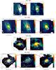Fig. 1

Σ_H₂ contours in M_⊙ pc^-2 derived from ¹²CO(1−0), ¹²CO(2−1), and ¹²CO(3−2) overlaid on Σ_SFR images in M_⊙ yr^-1 kpc^-2 at the intrinsic spatial resolution of the ¹²CO data and with pixel sizes equal to the ¹²CO resolution. The beams are plotted (in yellow) in the lower left corners of maps and their values are listed in Table 2. (Δα, Δδ)-offsets are with respect to the dynamical center of each galaxy. Σ_H₂ contours are drawn starting from noise levels >3σ with contour spacings that are whole multiples of >3σ.

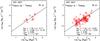Fig. 2

Left panel: K-S relation plot for NGC 3627 at the resolution of 82 pc. Σ_H₂ was derived from the ¹²CO(1−0) emission line map and Σ_SFR from the Hα image based on Eqs. (2) and (5), respectively. Red triangles indicate data points above 3σ significance both in Σ_H₂ and Σ_SFR, within a radius of 1.3 kpc (on the plane of the galaxy). The solid black line indicates the OLS bisector fitting line (see Sect. 3.7 for fitting method). The index N_fit and the intercept A_fit of the OLS bisector fitting line, the Pearson correlation coefficient r_core, and τ_depl values are reported in figure. Right panel: same as left panel with Σ_H₂ derived from the ¹²CO(2−1) emission line map based on Eq. (3) at the resolution of 36 pc. Red triangles indicate data points above 3σ significance both in Σ_H₂ and Σ_SFR, within a radius of 1.1 kpc (on the plane of the galaxy).

4.1. NGC 3627

NGC 3627 (Messier 66) is an interacting (e.g., Casasola et al. 2004) and barred galaxy classified as SAB(s)b at a distance of 10 Mpc, with signatures of a LINER/Seyfert 2 type nuclear activity (Ho et al. 1997). With NGC 3623 and NGC 3628, it forms the well-known Leo Triplet (M 66 Group, VV 308). Optical broad-band images of NGC 3627 reveal a pronounced and asymmetric spiral pattern with heavy dust lanes, indicating strong density wave action (Ptak et al. 2006). While the western arm is accompanied by weak traces of SF visible in Hα, the eastern arm contains a star-forming segment in its inner part (Smith et al. 1994; Chemin et al. 2003). NGC 3627 also possesses X-ray properties of a galaxy with a recent starburst (Dahlem et al. 1996). Both the radio continuum (2.8 cm and 20 cm, Urbanik et al. 1985; Paladino et al. 2008) and the CO emissions (e.g., Regan et al. 2001; Paladino et al. 2008; Haan et al. 2009; Casasola et al. 2011; Watanabe et al. 2011) show a nuclear peak, extending along the leading edges of the bar that forms two broad maxima at the bar ends, and then the spiral arms trail off from the bar ends. In contrast, the Hi emission exhibits a spiral morphology without signatures of a bar in the atomic gas (Haan et al. 2008; Walter et al. 2008). The derived gravity torque budget shows that NGC 3627 is a potential smoking gun of inner gas inflow at a resolution of ~60 pc (Casasola et al. 2011). In addition to ¹²CO lines, other molecular transitions have been detected in NGC 3627, including HCN(1−0), HCN(2−1), HCN(3−2), HCO⁺(1−0), and HCO⁺(3−2), suggesting the presence of high density gas (e.g., Gao & Solomon 2004; Krips et al. 2008).

The panels of the first line of Fig. 1 show the superposition of Σ_H₂ image contours derived from ¹²CO(1−0) and ¹²CO(2−1) emission lines overlaid on Σ_SFR images estimated from the Hα emission at the intrinsic resolutions of CO maps, i.e., ~1.̋7 (~82 pc) for the (1−0) transition and ~0.̋7 (~36 pc) for the (2−1) one. The value of Σ_H₂ has been derived from ¹²CO(1−0) and ¹²CO(2−1) emission lines by using Eqs. (2) and (3), respectively, and Σ_SFR by using Eq. (5). For ¹²CO(1−0) (left panel), the Σ_H₂ and Σ_SFR peaks are spatially coincident in the limit of the resolution of ~1.̋7 and the two distributions are quite consistent within a radius of ~3−4′′ (150−200 pc) from the nucleus (on the plane of the sky). At larger distances, Σ_H₂ and Σ_SFR are not correlated, mainly because Σ_SFR is not distributed along a bar as is Σ_H₂. Similar (anti-)correlations also characterize the comparison between Σ_H₂ derived from ¹²CO(2−1) emission line and Σ_SFR at the resolution of ~0.̋7 (right panel).

The lefthand panel of Fig. 2 shows the molecular K-S relation derived for NGC 3627 using the ¹²CO(1−0) emission line to estimate Σ_H₂ at the resolution of 82 pc. At this resolution the power index N_fit is equal to 1.18 ± 0.11 within a radius of 1.3 kpc (on the plane of the galaxy). Following the same procedure but convolving the original ¹²CO(1−0) and Hα maps at the lower resolution of 200 pc, the K-S relation has N_fit equal to 1.11 ± 0.41. The righthand panel of Fig. 2 shows the results obtained using the ¹²CO(2−1) emission line to derive Σ_H₂(Eq. (3)) at the resolution of 36 pc. At this resolution N_fit = 1.16 ± 0.05 within a radius of 1.1 kpc (on the plane of the galaxy), while N_fit increases to 1.59 ± 0.63 at the resolution of 200 pc. Although all the derived N_fit values are consistent with literature results (see later discussion in Sect. 5.1), the K-S relations studied at the resolution of 200 pc − for both ¹²CO(1−0) and ¹²CO(2−1) emission lines − with only four data points involved in the analysis do not allow us to infer statistical conclusions. In NGC 3627, we can only say that N_fit ≈ 1.2 both with Σ_H₂ derived from ¹²CO(1−0) at 82 pc and from ¹²CO(2−1) at 36 pc.

Neglecting the 200 pc-resolution cases, the Pearson correlation coefficient is ~0.6−0.7 and τ_depl is ~1.2−1.3 Gyr for both the lowest ¹²CO transitions.

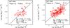Fig. 3

Left panel: same as left panel of Fig. 2 for NGC 4569 at the resolution of 154 pc. Red triangles indicate data points above 3σ significance both in Σ_H₂ and Σ_SFR, within a radius of 2.9 kpc (on the plane of the galaxy). Right panel: same as left panel with Σ_H₂ derived from the ¹²CO(2−1) emission line map at the resolution of 74 pc. Red triangles indicate data points above 3σ significance both in Σ_H₂ and Σ_SFR, within a radius of 2.1 kpc (on the plane of the galaxy).

4.2. NGC 4569

NGC 4569 (Messier 90) is a bright SAB(rs)ab galaxy at a distance of 17 Mpc in the Virgo cluster. A large scale bar is seen in NIR images (Laurikainen & Salo 2002) and is almost aligned with the major axis of the galaxy (PA = 15 deg according to Jogee et al. 2005). The galaxy harbors a nucleus of the transition type (type T2 in Ho et al. 1997), which exhibits a pronounced nuclear starburst activity. Hi emission line observations have revealed that in NGC 4569 the atomic gas is distributed along a central bar with radius of ~60′′ (~5 kpc, Haan et al. 2008). Interferometric CO observations of NGC 4569 presented previously (e.g., Helfer et al. 2003; Jogee et al. 2005; Nakanishi et al. 2005; Boone et al. 2007) have shown that the major part of the molecular gas detected in the inner 20′′ is concentrated within a radius of 800 pc, distributed along the large scale stellar bar seen in NIR observations, and with a peak close to the center and another one at ~500 pc from it. A hole in the CO distribution coincides with the nucleus where most of the Hα emission and blue light are emitted (Pogge et al. 2000). Boone et al. (2007) also demonstrate that the gravitational torques are able to efficiently funnel the gas down to ~300 pc.

The panels of the second line of Fig. 1 show the comparison between Σ_H₂ and Σ_SFR distributions in NGC 4569 at resolutions of ~1.̋9 (~154 pc from ¹²CO(1−0)), ~0.̋9 (~74 pc from ¹²CO(2−1)), and ~2.̋3 (~190 pc from ¹²CO(3−2)). The case involving the ¹²CO(3−2) emission line refers to Eq. (4) for deriving Σ_H₂. From these overlays it can be seen that Σ_H₂ and Σ_SFR are differently distributed at the available resolutions. While Σ_SFR is centrally concentrated and peaked, Σ_H₂ (derived both from ¹²CO(1−0) and ¹²CO(2−1) emission line) is distributed along a large scale bar of ~17′′× 6′′ (~1.4 kpc × 0.5 kpc) in size (in the plane of the sky) whose peak is far away from the peak of Σ_SFR. The same distribution is also visible in the SMA ¹²CO(3−2) map. There are, however, differences, perhaps due to the lower signal-to-noise ratio of the ¹²CO(3−2) SMA data relative to the IRAM observations (Boone et al. 2011).

Similar to NGC 3627, NGC 4569 exhibits a centrally concentrated morphology in the Σ_SFR images and a bar-like distribution in the Σ_gas maps. This could mean that the action of the bar has transported the gas to the nuclear regions to fuel a mini-starburst episode as found in many nearby spiral galaxies (Sakamoto et al. 1999).

Figure 3 and the lefthand panel of Fig. 6 show the molecular K-S relation derived for NGC 4569 with Σ_H₂ estimated from the three lowest ¹²CO emission lines at the intrinsic resolution of the ¹²CO maps. These figures, together with findings collected in Table 4, show that NGC 4569 has an index N_fit of the K-S relation that is sublinear (~0.6−0.7) for the three available ¹²CO transitions studied at spatial scales from 74 to 200 pc (producing six subcases), roughly constant as a function of resolution for a given ¹²CO transition, and only slightly varying as a function of ¹²CO transition at a resolution of 200 pc.

For NGC 4569, the Pearson correlation coefficient is approximately invariant with respect to the resolution, from 74 to 200 pc, for a given ¹²CO transition. In contrast to this, r_corr varies as a function of ¹²CO line at a given resolution (i.e., 200 pc). The best r_corr is obtained with the ¹²CO(2−1) line (~0.5−0.6), while the worst one with the ¹²CO(3−2) transition (~0.3) (¹²CO(1−0) gives r_corr~0.4).

As in NGC 3627, NGC 4569 has a short molecular τ_depl of ~1 Gyr, suggesting that the gas is efficiently converted in stars. Within a radius of 0.5 kpc, τ_depl is even smaller assuming values of ~0.7−0.9 Gyr.

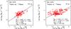Fig. 4

Left panel: same as left panel of Fig. 2 for NGC 4579 at the resolution of 154 pc. Red triangles indicate data points above 3σ significance both in Σ_H₂ and Σ_SFR, within a radius of 2.7 kpc (on the plane of the galaxy). Right panel: same as left panel with Σ_H₂ derived from the ¹²CO(2−1) emission line map at the resolution of 76 pc. Red triangles indicate data points above 3σ significance both in Σ_H₂ and Σ_SFR, within a radius of 1.5 kpc (on the plane of the galaxy).

4.3. NGC 4579

NGC 4579 (Messier 58) is a SAB(rs)b galaxy classified as an intermediate type 1 object (LINER/Seyfert 1.9) by Ho et al. (1997) at a distance of 20 Mpc in the Virgo cluster. It also has an unresolved nuclear hard X-ray (variable) source with a prominent broad Fe Kα line (Terashima et al. 2000; Ho et al. 2001; Eracleous et al. 2002; Dewangan et al. 2004). A non-thermal radio continuum source is detected at the position of the AGN (Hummel et al. 1987; Ho & Ulvestad 2001; Ulvestad & Ho 2001; Krips et al. 2007). The NIR K-band image of NGC 4579 has revealed a large-scale stellar bar and a weak nuclear oval (García-Burillo et al. 2009). The 21 cm Hi line observations have shown that the atomic gas in NGC 4579 is currently piling up in a pseudo-ring (radius of ~40′′, ~4 kpc) formed by two winding spiral arms that are morphologically decoupled from the bar structure (Haan et al. 2008). Molecular gas in the inner r ≤ 2 kpc disk is distributed in two spiral arms, an outer arc and a central lopsided disk-like structure (García-Burillo et al. 2009). The derived gravity torque budget in NGC 4579 have shown that inward gas flow is occurring on different spatial scales in the disk, with clear smoking gun evidence of inward gas transport down to r ~ 50 pc.

The panels of the third line of Fig. 1 show that in NGC 4579, Σ_H₂ and Σ_SFR have completely different distributions distributions at resolutions of both ~1.̋6 (~154 pc from ¹²CO(1−0)) and ~0.̋8 (~76 pc from ¹²CO(2−1)). The distribution of Σ_SFR is centrally concentrated within the inner ~4′′ (on the plane of the sky) and, at larger distances from the center, lies along two spiral arms extending up to ~12′′ from the nucleus. The morphology of Σ_H₂ traced by ¹²CO(1−0) and ¹²CO(2−1) is instead mainly defined by two highly contrasted spiral lanes without a central peak (García-Burillo et al. 2009).

Figure 4 shows the results obtained from the analysis of the K-S relation for NGC 4579. The value of N_fit ranges from ~0.5 to ~1.1 on spatial scales of 76−200 pc and considering ¹²CO(1−0) and ¹²CO(2−1) lines for Σ_H₂ derivation. For a given ¹²CO line, N_fit decreases with finer resolution. While for ¹²CO(1−0) N_fit gradually decreases from ~0.9 at 200 pc-resolution to ~0.8 at 154 pc-resolution, for ¹²CO(2−1) the decreasing of N_fit is stronger, from 1.1 to 0.5, possibly because the change from 200 to 76 pc in resolution is more drastic. At the common resolution of 200 pc, N_fit increases with higher J-CO transition.

In NGC 4579, the quality of the correlation tends to worsen with resolution. While for ¹²CO(1−0) r_corr is approximately constant (~0.6) through 154−200 pc resolution, for ¹²CO(2−1) it drops down from 0.6 to 0.5 in the resolution range from 200 to 76 pc. The correlation coefficient r_corr does not seem to depend on the CO transition, since it is ~0.6 for both ¹²CO lines at the common resolution of 200 pc.

Unlike NGC 3627 and NGC 4569, NGC 4579 has a more “standard” molecular τ_depl of ~2 Gyr (see later discussion in Sect. 5.2), without a radial trend. The similar trends obtained for N_fit and r_corr as a function of the resolution and for both the two lowest ¹²CO transitions suggest that in NGC 4579 the K-S relation is almost invariant with respect to ¹²CO(1−0) and ¹²CO(2−1) emission lines, but it changes slightly with spatial resolution.

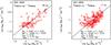Fig. 5

Left panel: same as left panel of Fig. 2 for NGC 4826 at the resolution of 56 pc. Red triangles indicate data points above 3σ significance both in Σ_H₂ and Σ_SFR, within a radius of 1.1 kpc (on the plane of the galaxy). Right panel: same as left panel with Σ_H₂ derived from the ¹²CO(2−1) emission line map at the resolution of 17 pc. Red triangles indicate data points above 3σ significance both in Σ_H₂ and Σ_SFR, within a radius of 0.6 kpc (on the plane of the galaxy).

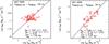Fig. 6

Left panel: same as Fig. 3, for NGC 4569, with Σ_H₂ derived from the ¹²CO(3−2) emission line map based on Eq. (4) at the resolution of 190 pc. Red triangles indicate data points above 3σ significance both in Σ_H₂ and Σ_SFR, within a radius of 2.9 kpc (on the plane of the galaxy). Right panel: same as left panel for NGC 4826 at the resolution of 59 pc. Red triangles indicate data points above 3σ significance both in Σ_H₂ and Σ_SFR, within a radius of 1.0 kpc (on the plane of the galaxy).

4.4. NGC 4826

NGC 4826, also known as the “Black Eye” or “Evil Eye” galaxy due to its optical appearance, is the closest target (~5 Mpc) of the NUGA core sample, and its nucleus is classified as a LINER type (Ho et al. 1997). It hosts two nested counter-rotating atomic and molecular gas disks of comparable mass (~10⁸ M_⊙, Braun et al. 1992, 1994; Casoli & Gerin 1993). The inner disk has a radius of ~50′′ (~1.3 kpc), while the outer one from ~80′′ to ~9.́8 (~2.1−15.3 kpc). By studying the stellar kinematics along the principal axes of NGC 4826, Rix et al. (1995) found that the stars rotate at all radii in the same direction as the inner disk, providing strong evidence that stars and gas are coplanar. NUGA observations have shown a high concentration of molecular gas (in ¹²CO(1−0), ¹²CO(2−1), and ¹²CO(3−2)), within a radius of 80 pc, forming a circumnuclear molecular disk. A detailed analysis of the kinematics, however, does not reveal any evidence of fueling of the nucleus.

The panels of the fourth line of Fig. 1 show the comparison between Σ_H₂ and Σ_SFR distributions in NGC 4826 at a resolution of ~2.̋1 (~56 pc from ¹²CO(1−0)), ~0.̋7 (~17 pc from ¹²CO(2−1)), and ~2.̋3 (~59 pc from ¹²CO(3−2)). Unlike NGC 4569 and NGC 4579, the morphologies of Σ_SFR and Σ_H₂ in NGC 4826 are spatially coincident and characterized by a structured disk.

Figure 5 and the righthand panel of Fig. 6 show the molecular K-S relation derived for NGC 4826 with Σ_H₂ estimated from the three lowest ¹²CO emission lines at the intrinsic resolution of the gas maps. As in NGC 3627, there are some cases where only four or five data points are involved in the analysis (¹²CO(2−1) and ¹²CO(3−2) at 200 pc). Neglecting these cases, the K-S relation derived from ¹²CO(1−0) shows that N_fit decreases from ~1.3 at 200 pc-resolution to ~0.9 at 56 pc-resolution. The case with ¹²CO(1−0) at 200 pc has a superlinear N_fit, while those analyzed at the intrinsic resolution of the all three ¹²CO maps (17−59 pc) are sublinear. The comparison between the K-S relation with ¹²CO(1−0) at 56 pc and that with ¹²CO(3−2) at 59 pc gives an almost identical N_fit (~0.9).

The good agreement between Σ_SFR and Σ_H₂ distributions (Fig. 1) consequently corresponds to a high Pearson correlation coefficient, equal to ~0.7−0.8 for all the cases with more than five data points at resolutions of 56−200 pc. These values of r_corr are the best in our sample of galaxies, and those of r_corr drop down to ~0.5 in the case using the ¹²CO(2−1) line at 17 pc, the highest resolution available not only in NGC 4826 but also in the present study. This drop of r_corr could be due to the high resolution; however, the comparison with the K-S relationship derived using the ¹²CO(2−1) line at 200 pc is not definitive proof of this because of the poor number statistics. For other sample galaxies (NGC 4569 and NGC 4579), there is no a strong difference in r_corr between ¹²CO(1−0) and ¹²CO(2−1). In addition to N_fit, r_corr also assumes similar values (0.7−0.8) in the cases of ¹²CO(1−0) at 56 pc and ¹²CO(3−2) at 59 pc. The results obtained for N_fit and r_corr therefore suggest that NGC 4826 has a K-S relationship independent of the ¹²CO transition at resolutions as high as ~60 pc.

Like NGC 4579, NGC 4826 has a τ_depl of ~2 Gyr without radial trend both by using ¹²CO(1−0) and ¹²CO(2−1), when taking only the statistically significant cases into account. The use of the ¹²CO(3−2) line instead gives a shorter τ_depl, of ~1 Gyr, and radial trend since it goes from ~1 Gyr within r< 1.0 kpc to ~0.7 Gyr within r< 0.2 kpc.

5. The molecular star-formation relation across the sample

The analysis performed for each galaxy showed a wide range of behaviors in terms of the K-S relations, and there is no “universal” molecular SF relation although the investigated galaxies belong to the same subclass of objects (i.e., nearby active galaxies), and all the derived quantities have been treated with the same methodology and at comparable spatial resolutions. The main result is therefore that each galaxy has its own SF relation (with its own index N_fit, correlation coefficient, and τ_depl) on spatial scales of ~20−200 pc. Nevertheless, we identified some common behaviors in terms of K-S relation, as discussed below.

5.1. The K-S relation index: resolution vs. ¹²CO transitions

By using the three lowest ¹²CO at resolutions of ~20−200 pc, we found K-S relation indexes N_fit ranging from ~0.5 to ~1.6, which are all values that are consistent with literature results. A superlinear slope of the K-S relation is consistent both with the early global disk studies of the SF relation by Kennicutt (1998a) and Kennicutt (1998b) based on the combination of atomic and molecular gas data for the Σ_gas computation and with more recent works based only on molecular component at sub-kpc scales (e.g., Kennicutt et al. 2007; Verley et al. 2010; Liu et al. 2011; Rahman et al. 2011; Momose et al. 2013). Bigiel et al. (2008) instead derived N ≈ 1 from the correlation between Σ_SFR and Σ_H₂ estimated from ¹²CO(2−1) data for seven nearby spiral galaxies. As already mentioned in Sect. 1, Bigiel et al. (2008) suggest that a linear correlation is evident in regions of high gas surface densities where the gas is typically molecular (≳10 M_⊙ pc^-2). Other studies using ¹²CO(2−1) also show a linear correlation (e.g., Leroy et al. 2008; Schruba et al. 2011), including one that combined single-dish ¹²CO(2−1) data with interferometric ¹²CO(1−0) data (Rahman et al. 2011). These ¹²CO(2−1) studies analyzed a substantial number of nearby galaxies, though it should be recognized that some studies based on ¹²CO(1−0) data showed a superlinear (power-law) correlation, rather than a linear correlation (e.g., Wong & Blitz 2002; Kennicutt et al. 2007; Liu et al. 2011). This suggests that the choice of the CO transition for deriving Σ_H₂ could affect N_fit values (see Bigiel et al. 2008). A linear slope has also been found by Vutisalchavakul et al. (2014) for the SF relation in an 11 deg² region of the Galactic plane with dust continua at 1.1 mm and 22 μm emission used as tracers of molecular gas and SFR, respectively, over a range of resolution from 33′′ to 20′ (~0.1−45 pc).

The most common explanation for a linear K-S relationship is that the observed CO luminosity is directly proportional to the number of star-forming clouds or GMCs, with all clouds having similar properties, such as the volume density, the efficiency of the cloud, and the SFR. In observations at resolution ≳100 pc, the individual clouds are not resolved but rather their CO flux is dispersed throughout the beam. In this case, regions with more clouds emit more CO in proportion to the number of clouds. Other recent works favor a sublinear (N ~ 0.6−0.8) K-S relationship at resolutions ≳170 pc (e.g., Blanc et al. 2009; Ford et al. 2013; Shetty et al. 2013, 2014a). A sublinear K-S relationship, in contrast to a linear one, suggests that the clouds do not have the same properties, and SFRs and/or volume densities vary (Shetty et al. 2014b). This means that there is no one-to-one correspondence between the CO luminosity and the number of clouds. In addition, the conversion factor X_CO also varies with the location in a galaxy (see later Sect. 6.1). Finally, a more straightforward explanation for the sublinear K-S relationship would be that CO permeates the hierarchical interstellar medium, including the filaments and lower density regions within which GMCs are embedded (Shetty et al. 2013, 2014b).

From Table 4 it emerges that for a given ¹²CO transition, the index N_fit tends to gradually decrease with finer resolution down to a resolution of approximately 20 pc. On the other hand, on scales larger than ~100 pc, the slope of the SF relation tends to increase and become somewhat superlinear. This result is common to all three lowest ¹²CO transitions and to all galaxies except for NGC 4569 whose N_fit is almost constant as a function of resolution as shown in the previous section. Our study therefore suggests that ~80−100 pc is the scale at which the K-S relation undergoes a change, both with respect to kpc scales and slightly finer spatial scales (≲250 pc, e.g., Bigiel et al. 2008, and this work). This contrasts with previous results by Onodera et al. (2010) for the Local Group spiral galaxy M 33, in which the slope steepens, and the correlation virtually disappears on small spatial scales of ~80 pc (i.e., GMC scales). However, in M 33, both the SFR and gas surface densities at 80 pc resolution are significantly lower than in the NUGA sample.

Table 4

Derived parameters from the pixel-by-pixel molecular star-formation relation for each galaxy.

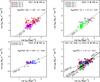Fig. 7

K-S relation plot for all sample galaxies. The top left panel plots all galaxies and only ¹²CO(1−0) emission line data; the top right panel all galaxies and only ¹²CO(2−1) emission line data; the bottom left panel all galaxies and only ¹²CO(3−2) emission line data; and the bottom right panel all galaxies and all the available ¹²CO emission line data, at the common spatial resolution of 200 pc. Different symbols and/or colors indicate galaxies whose Σ_H₂ has been derived from a given ¹²CO transition, as shown in the labels. The black lines refer to the OLS fits derived for different cases: the short-dotted line is for all galaxies and ¹²CO(1−0) emission line data, the point-dotted line for all galaxies and ¹²CO(2−1), the long-dotted line for all galaxies and ¹²CO(3−2), and the black solid line is for all galaxies and all the available ¹²CO lines. In the bottom right panel the ¹²CO(2−1) OLS fit line is hidden by total OLS fit line.

For distinguishing effects on the K-S relation index of different ¹²CO transitions to derive Σ_H₂, data are needed at a common resolution, 200 pc in the present work. The results from this comparison are displayed and collected in Fig. 7 and Table 5, respectively. Each panel of Fig. 7 shows the K-S relation plot for all sample galaxies and taking the three ¹²CO lines into account both separately and all together without distinction based on the transition. Different symbols and/or colors indicate galaxies whose Σ_H₂ has been derived from a given ¹²CO transition, and the black lines refer to the OLS fits derived for different cases. At the resolution of 200 pc, taking all sample galaxies into account and ¹²CO(1−0) (top left panel) and ¹²CO(2−1) (top right panel) separately, the resulting K-S relations have indices of 1.20 ± 0.03 and 1.14 ± 0.01, respectively. These findings indicate that ¹²CO(1−0) and ¹²CO(2−1) lines lead to quite similar results in terms of the slope of the K-S relation. Under the same conditions but by using ¹²CO(3−2) data (bottom left panel), we found a sublinear slope of 0.67 ± 0.02. However, this result is based only on two cases, NGC 4569 and NGC 4826, and for NGC 4569 all slopes for the three lowest ¹²CO transitions at all investigated resolutions (74−200 pc) are sublinear. In contrast, in NGC 4826 the slope derived from the ¹²CO(3−2) line is roughly unity at 200 pc of resolution (see Table 4). Taking all sample galaxies and all available ¹²CO transitions (bottom left panel) into account, the K-S relation has a “standard” index of 1.14 ± 0.01.

It is well known that each transition traces different physical gas properties. The kinematic temperature of molecular gas is typically ~10 K (Scoville et al. 1987), which is above the level energy temperature of 5.5 K for the J = 1 level of the ¹²CO, but below the temperatures of 16.5 K and 33 K for the J = 2 and J = 3 levels, respectively. This implies that a slight change in gas kinematic temperature is sufficient to affect the excitation for the ¹²CO(2−1) and ¹²CO(3−2) emission lines. The different critical densities of the three ¹²CO transitions (~10³ cm^-3, ~2 × 10⁴ cm^-3, and ~7 × 10⁴ cm^-3 for ¹²CO(1−0), ¹²CO(2−1), and ¹²CO(3−2), respectively) make their line ratios sensitive to local gas density. The value of R₂₁ has been observed to systematically vary with SFR and Σ_gas in the Milky Way (e.g., Sakamoto et al. 1995; Sawada et al. 2001) and M 51 (Koda et al. 2012; Vlahakis et al. 2013). Despite this, because of the use of individually measured mean R₃₂ to convert to an equivalent CO(1−0) mass conversion, such variations do not have a significant impact on the resulting index N_fit of the K-S relation.

Another result emerging from Table 4 concerns the K-S relation studied at 200 pc resolution with Σ_H₂ derived from ¹²CO(1−0). NGC 3627, NGC 4579, and NGC 4826 exhibit K-S relations with indices N_fit around unity, with Σ_H₂ of ~20−100 M_⊙ pc^-2, and τ_depl of ~1.5−2 Gyr. NGC 4569 is different from the other sample galaxies also in this respect; it indeed has a Σ_H₂ of ~50 M_⊙ pc^-2, comparable to the other galaxies, but its K-S relation has a sublinear slope and τ_depl of ~1 Gyr.

Table 5

Derived parameters from the pixel-by-pixel molecular star-formation relation across the sample at the common spatial resolution of 200 pc.

5.2. The molecular gas depletion time

As discussed in Sect. 1, τ_depl is an important parameter in the study of the K-S relation, as is the power index N_fit, for understanding the SF phenomenon in galaxies. We found molecular τ_depl ranging from ~1 to ~2 Gyr, which is consistent with more recent results as discussed below. Each galaxy has its own τ_depl that seems to be invariant with respect to the spatial scale probed in a given galaxy, at resolutions from ~20 to 200 pc. The molecular τ_depl is also invariant with respect to ¹²CO(1−0) and ¹²CO(2−1) lines. The discussion of the τ_depl derived from ¹²CO(3−2), for NGC 4569 and NGC 4826, deserves separate treatment and is discussed later.

Both NGC 3627 and NGC 4569 have molecular τ_depl of ~1−1.3 Gyr, by using ¹²CO(1−0) and ¹²CO(2−1) and taking only the statistically significant cases into account. These values of τ_depl are compatible with the mean molecular [¹²CO(1−0)] τ_depl of ~1.2 Gyr (with α_CO = 3.5 M_⊙ (K km s^-1 pc^-2)^-1) found by Saintonge et al. (2011) for the COLD GASS sample of more than 200 galaxies at distances of ~100−200 Mpc, but lower than the mean molecular [¹²CO(2−1)] τ_depl of ~2 Gyr found by Bigiel et al. (2008) and Leroy et al. (2008) in the HERACLES survey consisting of a sample of 48 nearby (D ~ 3−20 Mpc) galaxies. NGC 3627 and NGC 4569 therefore have a τ_depl that is more consistent with the COLD GASS single-dish survey that gives a global picture of gas and SF in the Local Universe but lacks the power to trace the exact distribution of these components, rather than with the HERACLES survey, which like the present study, maps them. However, Saintonge et al. (2011) demonstrate that after using the same conversion factor from CO luminosity and H₂ mass (α_CO = 3.5 M_⊙ (K km s^-1 pc^-2)^-1) and restricting the HERACLES sample to the COLD GASS stellar mass range, the mean molecular τ_depl for HERACLES is ~1 Gyr, which is consistent with the COLD GASS estimate.

As mentioned in Sect. 4.2, τ_depl of NGC 4569 also shows a hint of radial trend-reaching values of ~0.7−0.9 Gyr within a radius of 0.5 kpc. These low values for the molecular τ_depl are also in line with the recent results by Faesi et al. (2014) for NGC 300 on 250 pc scales, so slightly larger than but comparable to ours, and by Lada et al. (2010) for the Milky Way GMCs, who found depletion times of ~0.2 Gyr. After Faesi et al. (2014) studied the relation between molecular gas and SF in 76 Hii regions of NGC 300, they concluded that the short τ_depl arises because their analysis accounts for only the gas and stars within the youngest star-forming regions. These depletion times correspond to the timescale for SF to consume the gas reservoir in the star clusters’ parent GMCs, which may be the more relevant quantity in the context of GMC-regulated SF in galaxies.

The hint of a radial trend of τ_depl in NGC 4569 also suggests that SF becomes more inefficient at larger radii under the assumption of a fixed X_CO conversion factor. This finding agrees with results obtained by Leroy et al. (2013) who find systematically lower τ_depl for a given X_CO in the inner kpc of a sample of 30 galaxies, among AGN and starbursts. Since X_CO is typically smaller when closer to galaxy nuclei (Sandstrom et al. 2013), implying shorter τ_depl for a given CO luminosity, the radial trend in τ_depl could be even steeper. The shortening of τ_depl toward the very center of NGC 4569 coincides both with a better correlation between Σ_H₂ and Σ_SFR distributions (see Fig. 1) and with an increase in the R₂₁ ratio there, which is indicative of more excited gas. The value of R₂₁ ranges from 0.2 to 0.9 in the inner region of NGC 4569 (Boone et al. 2007, 2011), with a smooth and fairly symmetric distribution with respect to the center, and continuously increasing toward the nucleus.

Similar radial trends in R₂₁ that are also present in other NUGA galaxies (NGC 4579, NGC 6574: García-Burillo et al. 2009; Lindt-Krieg et al. 2008, respectively) and in the sample of Leroy et al. (2013) presumably reflect similar changing physical conditions that drive the lower X_CO factors found by Sandstrom et al. (2013). This would underscore that molecular gas in the central regions gives off more CO emission, appears more excited, and forms stars more rapidly than molecular gas farther out in the disks of galaxies. Compared to R₂₁, R₃₂ shows a clumpier and more asymmetric distribution within the central region (Boone et al. 2011), differently from the large-scale gradient in R₃₂ reported by Wilson et al. (2009). Usually, R₃₂ is expected to probe more extreme physical conditions, such as those occurring in star-forming or shock regions. Boone et al. (2011) indeed confirm that R₃₂ tracks massive SF in NGC 4569 better than R₂₁ by comparing R₂₁ and R₃₂ maps to the Paα image as detected by NICMOS (see also Wilson et al. 2009). In any case, in NGC 4569, ¹²CO is less excited (R₃₂ ~ 0.6) than in the Galactic center and in most of the centers of normal, starburst, and active galaxies studied so far for which R₃₂ ≈ 0.2−5 (e.g., Devereux et al. 1994; Mauersberger et al. 1999; Matsushita et al. 2004; Mao et al. 2010; Combes et al. 2013; García-Burillo et al. 2014). Shorter τ_depl could also be due to the high pressure driven by the deep potential well in the central parts of galaxies, driving gas to higher densities. This effect has been seen both in our Galaxy (Oka et al. 2001) and in others (Rosolowsky & Blitz 2005), and it has been suggested that it explains shorter τ_depl (i.e., enhanced SFE in galaxy centers) in the sample of Leroy et al. (2013).

NGC 4579 and NGC 4826 instead have higher molecular τ_depl of ~2 Gyr, both with ¹²CO(1−0) and ¹²CO(2−1) when only taking the statistically significant cases into account. For NGC 4579, neglecting the case of the net sublinear K-S relationship found with ¹²CO(2−1) at the resolution of 76 pc, τ_depl~ 2 Gyr is accompanied by an index N_fit around unity. As already mentioned above, the interpretation of a linear K-S relationship is that CO is primarily tracing star-forming clouds with relatively uniform properties, including Σ_SFR, and consequently the τ_depl of the CO traced gas is constant and of ~2 Gyr, both within and between galaxies. However, there is still no consensus on either the precise K-S parameter estimates or the associated interpretation (see Dobbs & Pringle 2013, for a review of explanations of the K-S relationship). In contrast to NGC 4569, τ_depl in NGC 4579 does not show a radial trend although R₂₁ varies as a function of the radius. Close to the AGN, at r< 200 pc, R₂₁≈0.8−1, whereas at r> 500 pc R₂₁≈0.4−0.6 (García-Burillo et al. 2009).

The use of the ¹²CO(3−2) line gives a τ_depl of ~1 Gyr both for NGC 4569 and NGC 4826, suggesting that the gas traced by this transition could be more efficiently converted into stars with respect to ¹²CO(1−0) and ¹²CO(2−1) emissions, despite using mean CO(1−0)/CO(3−2) ratios to convert mass densities. While NGC 4569 has τ_depl~ 1 Gyr for all three ¹²CO lines and for all resolutions taken into account, NGC 4826 shows a lower ¹²CO(3−2) τ_depl than those derived from ¹²CO(1−0) and ¹²CO(2−1) (~2 Gyr). In addition, for NGC 4826, this trend is seen by using ¹²CO(3−2), while τ_depl does not show a radial trend in the cases of ¹²CO(1−0) and ¹²CO(2−1). However, the ¹²CO(3−2) distribution is similar to that of the CO(1−0) and CO(2−1) lines at the same resolution (Boone et al. 2011). In contrast to NGC 4569, R₃₂ does not appear to be clumpier than R₂₁ in NGC 4826, and both maps look relatively symmetric with respect to the dynamical center, with both ratios increasing steadily toward the center (Boone et al. 2011). As in NGC 4569, high R₃₂ values (>0.3) occur within the Paα emission region as detected by NICMOS, while this is not true for R₂₁, which reaches high values (>0.7) away from the Paα emitting regions (Boone et al. 2011). This difference, along with the variation in R₃₂, could be responsible for the short τ_depl inferred by ¹²CO(3−2) in NGC 4826.

Table 6

Stellar and star formation properties of our galaxy sample.

Compared to the ¹²CO(1−0) and ¹²CO(2−1), the ¹²CO(3−2) traces relatively warmer and denser gas. There is also growing evidence that the ¹²CO(3−2) emission correlates more tightly with the SFR or SFE than does ¹²CO(1−0) and ¹²CO(2−1) (e.g., Komugi et al. 2007; Muraoka et al. 2007; Wilson et al. 2009, 2012). Similarly, Iono et al. (2009) show that the ¹²CO(3−2) emission correlates nearly linearly with the FIR luminosity for a sample of local luminous IR galaxies and high-redshift submillimeter galaxies. Thus, it appears that the ¹²CO(3−2) emission primarily traces the molecular gas associated directly with SF, such as high-density gas that is forming stars or warm gas heated by SF, rather than the total molecular gas content of a galaxy usually traced by ¹²CO(1−0) and ¹²CO(2−1). Nevertheless, this evidence is not able to explain the shorter τ_depl characterizing the ¹²CO(3−2)-molecular K-S relation for NGC 4826 with respect to ¹²CO(1−0) and ¹²CO(2−1).

Values of τ_depl derived for a given galaxy and within comparable FoVs are indeed expected to be similar for all ¹²CO lines, by construction, since we are not deriving gas traced by ¹²CO(3−2) but rather the total gas, assuming a R₃₂ line ratio, in addition to the X_CO conversion factor (see Eq. (4)). The bottom righthand panels of Figs. 7 and 8 show that Σ_H₂ data points derived from the ¹²CO(3−2) line emission have typically lower Σ_H₂ values with respect to ¹²CO(1−0) and ¹²CO(2−1) derivation, but this effect is not due to the choice of the ¹²CO line but simply to the availability of ¹²CO(3−2) data only for NGC 4569 and NGC 4826. It is possible that our result is simply due to the variation in R₃₂ that could not be considered in the mean value used for the derivation of Σ_H₂ in Eq. (4).

The radial trend of τ_depl as a function of physical conditions of gas, typically expressed in terms of line ratios, is not clearly defined. While NGC 4569 exhibits a τ_depl that decreases toward the very center, together with an increase in R₂₁, NGC 4579 has constant τ_depl as a function of the radius but higher R₂₁ in the central galaxy region. This difference could be explained by the (dis)agreements between gas and SFR morphologies for the two galaxies. Both NGC 4569 and NGC 4579 are centrally peaked in Σ_SFR without a counterpart in Σ_H₂ (see Fig. 1). However, NGC 4569 shows CO emission in the very center, but NGC 4579 has neither gaseous nuclear emission nor a radial trend in the gas morphology (although the R₂₁ line ratio decreases as a function of radius). It appears therefore that the radial trend of τ_depl as a function of CO line ratios also has to be accompanied by similar radial trends in both gas and SFR morphologies in a given galaxy.

It is well known that gas depletion times are different in extreme starburst galaxies and merging systems in the Local Universe, as well as in submillimeter galaxies at high redshifts (e.g., Kennicutt 1998a; Bouché et al. 2007; Riechers et al. 2007; Bothwell et al. 2010). In these galaxies, gas depletion times are significantly shorter than the normal galaxy population, with the star formation surface density being an order of magnitude larger at fixed gas surface density (Genzel et al. 2010). More recently, it has emerged that the molecular τ_depl varies even within the population of nearby “normal” star-forming galaxies and that this variation has been quantified as a function of a range of fundamental parameters. Saintonge et al. (2011), Boselli et al. (2014), and Bothwell et al. (2014) all find that depletion timescales vary monotonically from ~2 Gyr to ~0.1 Gyr across two orders of magnitude in stellar mass. This finding also persists when using a constant conversion factor and different conversion factor values (Bothwell et al. 2014). Saintonge et al. (2011) also find that τ_depl correlates inversely with the specific SFR (SFR per unit stellar masses, sSFR). Table 6 collects the main stellar and star formation properties of our galaxy sample. In this table, Col. (1) gives the galaxy name, Col. (2) the logarithm of the stellar mass (M_∗), Col. (3) the logarithm of the total IR (TIR) luminosity, Col. (4) the SFR derived adopting the conversion of Kennicutt (1998a) for TIR (from 8−1000 μm), and Col. (5) the logarithm of the sSFR. NUGA galaxies have stellar masses in the COLD GAS range (log(M_∗) from 10 to 11.5 M_⊙) and sSFR toward the high end of the COLD GAS sample (log(sSFR) from −11.8 to −9.5 yr^-1), so are consistent both with our results for short depletion times and the correlation that Saintonge et al. (2011) find between τ_depl and sSFR. Nevertheless, the NUGA galaxies with the longest τ_depl (although only a factor of 2) have the highest sSFR, although the values are within the scatter found by Saintonge et al. (2011).

The dependence of τ_depl on the spatial scale has also been explored by other groups. Schruba et al. (2010) find a median τ_depl~1.1 Gyr for M 33 (using the conversion factor we use here) with no dependence on type of region targeted on kpc scales, but below these scales τ_depl is a strong function of both the adopted scale and the type of region that is targeted (see also Komugi et al. 2005, for τ_depl even down to 0.1 Gyr in the central few hundred parsecs of local spirals). Schruba et al. (2010) derived very long τ_depl (up to 10 Gyr) using small apertures centered on CO peaks, but very short τ_depl (0.3 Gyr) with small apertures targeted toward Hα peaks. This may not be surprising, given the disparity in the bright Hα and CO distributions in M 33 (see Fig. 1 in Schruba et al. 2010), similar to the inconsistencies between Σ_gas and Σ_SFR morphologies characterizing some NUGA galaxies, such as NGC 4569 and NGC 4579 (see Fig 1). Schruba et al. (2010) find that the SF relation in M 33 observed on kpc scales breaks down for aperture sizes of ~300 pc. These aperture sizes are larger than the breakdown scale of 80−100 pc found by Onodera et al. (2010) for the same galaxy.

5.3. The dispersion of the data

At the relatively high resolutions studied here, the Pearson correlation coefficient r_corr is generally low, and there is large scatter with values as low as ~0.3. Angular resolutions of ~1−2′′ correspond to ~20−200 pc at the distances of the sample galaxies. An inspection of the maps shown in Fig. 1 reveals that CO intensity peaks are offset from the Hα peak, often by more than ~1−2′′. In addition, there is the possibility that such small beams do not include both the star-forming region and its counterpart molecular cloud, which is generally several tens of parsecs in size. In general, star-forming regions do not coincide with the molecular clouds that give birth to them. This is typically seen in spiral arms of galaxies, where the optical and molecular spiral structures are offset. If only the molecular clouds are observed and not the star-forming regions which are physically coupled to them, the gas density would be expected to show an excess over the expected correlation.

For a given galaxy, for a given ¹²CO transition, and with only the statistically significant cases, r_corr is quite stable (see NGC 4569) or it tends to decrease with resolution, although this tendency is weak (see NGC 4579 in ¹²CO(2−1) and NGC 4826 in ¹²CO(1−0)). The latter trend is consistent with the result of a larger scatter on smaller scales found by Vutisalchavakul et al. (2014) when studying the SF relation in the Galactic plane. They found that the rank correlation coefficients between log(Σ_H₂) and log(Σ_SFR) increase from ~0.4 to ~0.8 in the resolution range from 33′′ to 20′. Vutisalchavakul et al. (2014) also compared their results with some resolved extragalactic SF relations, available on a scale of about 200 pc (for instance, M 33 from Schruba et al. 2010), finding the same trend of the dispersion as a function of resolution for extragalactic data and a smaller scatter in the depletion time distribution for the Galactic plane than for the extragalactic sources.

5.4. The K-S relation at high densities of molecular gas

The range of Σ_H₂ over which we studied the K-S relation is ~20−120 M_⊙ pc^-2. These densities are higher than those of 20−50 M_⊙ pc^-2 studied by Bigiel et al. (2008) and other authors. The circumnuclear regions examined here are subject to physical conditions that are different from the disk. Besides denser gas tracers, such as HCN and HCO⁺, observed in these regions (e.g., Krips et al. 2011; Combes et al. 2013, 2014; García-Burillo et al. 2014), rotation curves in the central kpc are different from disks, following roughly rigid-body rotation compared to nearly flat in the disks (e.g., Sofue et al. 2003). This would lessen the effect of shear, which works on the clouds, and may enhance the efficiency of the SF arising from gravitational collapse. These effects could conspire to produce a systematic change in the K-S relation in the central regions of galaxies. Figure 8 shows the comparison between our results for the whole sample at 200 pc resolution (as also displayed in Fig. 7) and the findings from Bigiel et al. (2008). Also plotted in Fig. 8 are the predictions from the Krumholz et al. (2009) models for solar metallicity and various clumping factors (see Krumholz et al. 2009, for more details). For the comparison we have converted the Σ_H₂ measurements in Bigiel et al. (2008) to the conversion factor we use here, but have not adjusted the SFRs since the Kroupa IMF (Kroupa 2001) used by them is similar to ours (see Calzetti et al. 2007). Figure 8 also shows two trends found by Genzel et al. (2010): the (blue) short-dashed line gives the common trend for star-forming galaxies (SFGs) and mergers/starburst using a single conversion factor (α_CO = 3.2 M_⊙ pc^-2 (K km s^-1)^-1); the (red) long-dashed line corresponds to the merger/starburst trend only (with α_CO = 1 M_⊙ pc^-2 (K km s^-1)^-1). Both regressions have been adjusted to our α_CO (3.5 M_⊙ pc^-2 (K km s^-1)^-1) and to our not including helium.

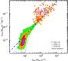Fig. 8

Comparison between (i) the K-S relation plot derived for all sample galaxies and taking all the ¹²CO emission lines at the common resolution of 200 pc into account, as shown in Fig. 7; and (ii) results from Bigiel et al. (2008). The model predictions from Krumholz et al. (2009) are also shown with solar metallicity and clumping factor c = 1, 2, and 5; see Krumholz et al. (2009) for more details. Also shown (as a blue short-dashed line) is the trend for star-forming galaxies and mergers found by Genzel et al. (2010) using a common conversion factor α_CO (=3.2 M_⊙ pc^-2 (K km s^-1)^-1). The horizontal axis has been adjusted to our α_CO (=3.5 M_⊙ pc^-2 (K km s^-1)^-1) and our non-inclusion of helium. We have also plotted the merger/starburst trend by Genzel et al. (2010) (with α_CO = 1 M_⊙ pc^-2 (K km s^-1)^-1) as shown by a (red) long-dashed line.

We find that at densities as high as ~10³ M_⊙ pc^-2 there is reasonable agreement with the predictions of Krumholz et al. (2009). However, with a common conversion factor, the central regions of the NUGA galaxies have higher Σ_SFR for a given gas column than would be expected from the models. They fill in the region between the mergers or high-z starburst systems and the more quiescent SFGs studied by Genzel et al. (2010), assuming that the former require a lower value of α_CO. The apparently high Σ_H₂ would also be consistent with the results of Sandstrom et al. (2013), who find that α_CO in centers of galaxies relative to their disks can be as much as ten times lower. We could thus be slightly overestimating Σ_H₂ in our sample, although it is difficult to determine by exactly how much. To assuage the offset between mergers or starbursts and SFGs, Krumholz et al. (2012) have devised a “universal SF law” that is based on volumetric densities (see also Genzel et al. 2010). They argue that such a formulation is particularly important for resolutions of 10−100 pc, similar to what is achieved by our observations. In addition, the galaxies studied here are roughly consistent with model predictions of Krumholz & McKee (2005) and Krumholz et al. (2009).

It is difficult to consider the K-S relation for normal galaxies at even higher densities. This would require that we observe with even better spatial resolution (possible with ALMA), but the GMCs would then be highly resolved. Thus we may not be able to observe the molecular cloud and its counterpart star-forming region within one beam, for galaxies − such as those studied here − at distances of ~5−20 Mpc (see Sect. 5.3). It is possible that the K-S relation is fundamentally a correlation that is seen only when the ISM is averaged over a considerable area. As already discussed in Sect. 5.1, our work shows that the K-S relation undergoes a change at a spatial resolution of ~80−100 pc (~GMC scale); i.e., its slope starts to decrease sharply with respect to higher scales. The breakdown of the K-S relation could therefore occur at ~80−100 pc, as found by Onodera et al. (2010) for M 33, even if in NUGA dense nuclei a net breakdown is still not visible on scales as high as ~20 pc.

6. Caveats

Here we examine possible caveats or systematic uncertainties associated with our analysis and results presented in the previous sections. These can arise from physical causes connected to our simplified assumptions, from the methodology we used to derive the various quantities, and/or from the adopted fitting method of data.

6.1. Derivation of Σ_H₂

It is well known that the X_CO conversion factor is a source of systematic uncertainty in the estimate of Σ_H₂. By adopting a constant value for X_CO, we do not account for its changes with galaxy properties, such as physical gas conditions and metallicity (e.g., Maloney & Black 1988; Bolatto et al. 2008; Glover & Mac Low 2011; Magrini et al. 2011; Bolatto et al. 2013). Estimates of “typical” values of X_CO in the Milky Way and other spiral galaxies range from ~1.5 × 10²⁰ cm^-2 (K km s^-1)^-1 to ~4 × 10²⁰ cm^-2 (K km s^-1)^-1.

CO line ratios are typically used to constrain the excitation conditions (temperature, density, and column density) of the line-emitting gas. Some studies have shown that these line ratios (mainly R₂₁) tend to radially vary, with higher values toward galaxy nuclei (e.g., Lindt-Krieg et al. 2008; García-Burillo et al. 2009), and this effect presumably reflects similar changing of the physical conditions that drive the lower X_CO factors found by Sandstrom et al. (2013). When presenting a review of the theoretical underpinning, techniques, and results of efforts to estimate X_CO conversion factor in different environments, Bolatto et al. (2013) also stress that X_CO appears to drop in the central, bright regions of some but not all galaxies.

The AGN may also play a role since a higher R₂₁ toward the center of active galaxies could be interpreted as evidence of external heating of molecular clouds by X-rays in the vicinity of the AGN (e.g., Baker et al. 2003). However, this radial trend of the gas physical conditions does not unambiguously characterize all the LLAGN in our sample. Although R₂₁ ratios show a radial trend, or hints of it, in NGC 4569, NGC 4579, and NGC 4826, R₂₁ in NGC 3627 and R₃₂ in NGC 4569 and NGC 4579 do not exhibit the same behavior when assuming a constant or stochastic variation as a function of radius. For the lack of a common trend in our sample, we adopted constant values of R₂₁ and R₃₂. This assumption may introduce an uncertainty into the Σ_H₂derivation, although NUGA galaxies benefit from individual measures of line ratios for each galaxy nuclear region.

As for metallicity, Boissier et al. (2003) and Narayanan et al. (2012) find that by using metallicity-dependent X_CO, Σ_H₂ should typically change by a factor of 2 to 3 in the central regions compared to disk regions of nearby spirals, in the sense of decreasing the gas mass. Our sample galaxies have all been observed by Moustakas et al. (2010), who find roughly solar metallicities for all but were unable to evaluate metallicity gradients for lack of data. Nevertheless, because of the relatively small FoV afforded by our CO observations, any metallicity gradient is expected to be very slight over the radial range sampled by our data. We therefore adopted a constant X_CO for the sake of uniformity and simplicity, as suggested in the review of Bolatto et al. (2013) in the absence of a detailed characterization of X_CO in a given galaxy and as typically done in the major portion of studies aimed at determining molecular gas mass from ¹²CO line intensities.

As already discussed in Sect. 1, we only used molecular (hydrogen) gas in our study based on the assumption that SF formation occurs in molecular cloud cores where H₂ dominates. This implies a two-step process of SF where H₂ clouds are first formed from Hi, and stars are then formed from H₂. This leads to the hypothesis that H₂ should be more directly connected with SFR. Moreover, we are interested in galactic centers that are high-density regions of galaxies and that can be Hi deficient (e.g., Bigiel et al. 2008). Haan et al. (2008) observed the atomic gas for the galaxies in our sample, but the Hi beam approximately subtends our entire CO FoV, ranging from ~20′′ to ~40′′. With this beam, NGC 4579 has an Hi central hole with a surrounding ring, and this galaxy also has the lowest ⟨Σ_H₂⟩ in our sample (see Table 4). For the other galaxies, Hi column densities Σ_HI≈ 10−13 M_⊙ pc^-2 for NGC 4569 and NGC 4826, and ~100 M_⊙ pc^-2 for NGC 3627. In the first two, mean Σ_H₂ are 20−40 times higher, so neglecting Hi will introduce a few percent systematic underestimate of gas surface density; nevertheless, the Hi beam is large so this could be an underestimate. NGC 3627 has the highest Σ_H₂ of our sample (600−700 M_⊙ pc^-2), but the dense Hi gas is still a relatively small fraction. In any case, as shown by the model predictions of Krumholz et al. (2009) in Fig. 8, Σ_H₂ in the NUGA galaxies even at 200 pc resolution are in the surface-density regime where H₂ is expected to dominate.

For most of CO data of our sample, it has been possible to combine interferometric data with single-dish ones, allowing the “missing flux” problem to be resolved (see Table 2). Because in a interferometer two antennas cannot be placed closer than some minimum distance (D_min), signals that are stronger than some value (∝λ/D_min) will be attenuated. For only interferometric ¹²CO maps can the spatially extended sources therefore not be detected, which would have the effect of underestimating the gas surface density.

6.2. Derivation of Σ_SFR: diffuse Hα, [N II] contamination, and Hα extinction

Our values of Σ_SFR inferred from Hα could be overestimated if some fraction of the emission not directly associated with ionization by massive stars were diffuse. Rahman et al. (2011) find that K-S slopes are steeper, the stronger the fraction of diffuse emission in the SFR tracer (see also Liu et al. 2011). However, they also conclude that diffuse emission either in the SFR tracer or in CO do not compromise results in the high column-density regions of the galaxy they studied, NGC 4254. Since NGC 4254 has peak Σ_H₂≲ 200 M_⊙ pc^-2, comparable to the mean Σ_H₂ of our sample galaxies, we do not expect the potential overestimate of SFR from diffuse Hα emission to be a significant problem.

We removed the [N ii] contamination within the filter bandpass using average [N ii]/Hα values available in the literature, as typically done in narrow-band studies. However, Blanc et al. (2009) used integral-field spectroscopy to study the spatially-resolved SF relation in NGC 5194, and checked the validity of the assumption of a constant [N ii]/Hα and the bias introduced by it. They find an increasing [N ii]/Hα ratio as one goes to fainter Hα fluxes, which is consistent with the nebular emission in the faintest parts of the galaxy (mainly in the interarm regions) being dominated by the diffuse ionized gas. Assuming a constant [N ii]/Hα may thus introduce an underestimation of the Hα flux (and therefore of the derived SFR) in the galaxy’s central regions.

In Sects. 1 and 3.3, we stressed that the Hα emission lines are subject to extinction within the galaxies, which we took into account for our analysis by adopting A_V(int) values determined for each sample galaxy rather than a mean value. However, we applied this throughout, as suggested by Kennicutt & Kent (1983). This is somewhat of an oversimplification because central regions of galaxies are generally subject to greater extinction than disk regions. This may cause the extinction correction and (therefore) the SFR to be underestimated.

6.3. Choice of the fitting method

A central component of observational investigations is also the quantification of the correlation between two or more observed quantities. Typically, linear regression provides estimates of the zero point and slope of the “best-fit” regression line between the observed data. Since each adopted methodology for fitting a power law to the data introduces a bias in the results, it is important to understand the limitations of common fitting methods. Usually in the K-S relation studies a linear regression in logarithmic space is performed, but methods differ in the treatment of error bars. Some works (e.g., Kennicutt et al. 2007; Rahman et al. 2011; Momose et al. 2013) used the FITEXY algorithm (Press et al. 1992), which has the advantage of incorporating errors in both the ordinate and abscissa coordinates, thus providing robust regression results, although errors must be assumed to be symmetric in logarithmic space, which is not always the case. Other studies, already quoted in Sect. 3.7 and including the present work, adopted the OLS bisector method, which returns a bisector line in x- and y-axes without the errors being taken into account. Both methods have the disadvantage of not being able to incorporate upper limits in the minimization.

For this reason, Blanc et al. (2009) introduced and used a new method for fitting, based on Monte Carlo approach combined with two-dimensional distribution comparison techniques, which is not affected by the above issue. This method has the strong advantage of including the regions not detected in the CO map, including those with negative measured fluxes, in addition to incorporating the intrinsic scatter in the SF relation as a free parameter and performing the fitting in linear space, thereby avoiding the assumption of log-normal symmetric errors. For a detailed discussion of the disadvantages of the linear regressions with respect to a Monte Carlo fitting method for a more realistic treatment of systematics and accurate determination of the parameters and errors, we refer the reader to Blanc et al. (2009) and Shetty et al. (2013). Such an analysis is beyond the scope of this paper.

Based on the IRAM PdBI CO data reduction performed for all NUGA galaxies, we preferred to take only data above 3σ level into account, for which we are certain of the interferometric significance. When analyzing the SF relation at sub-kpc scales of ten nearby galaxies, Momose et al. (2013) note that the choice of CO threshold surface density (3σ also in their case) affects the results very little; however when repeating the analysis with various thresholds, they obtained the same findings in terms of the K-S relation. Since we had compared our results with Bigiel et al. (2008) (see Fig. 8) who used the OLS bisector method, we also adopted it.

We note that results derived from the robust regression-fitting method can differ very much from OLS bisector ones (see Table 4), confirming that the choice of the fitting method affects the findings (Blanc et al. 2009; Shetty et al. 2013). This further reinforces the need to compare K-S relation results obtained based on the same fitting method.

7. Conclusions

We have investigated the resolved molecular K-S relation in the central kpc of four NUGA galaxies that have different types, which interact or do or not, which are barred or not, which have either a Seyfert or a Liner nucleus. Their SFR ranges from ~0.7 to ~4 M_⊙ yr^-1, and sSFR from 0.04 to 0.5 Gyr^-1. The spatial scales studied in this work lie between ~20 and 200 pc, and densities sampled are higher than in the usual galaxy disks, extending toward 100−1000 M_⊙ pc^-2.

The first result was that each galaxy has its own molecular SF relation on the investigated spatial scales. The K-S relation is most often underlinear (see NGC 4569), with slopes ranging from ~0.5 to ~1.3. The derived depletion time scales range between 1 and 2 Gyr, which is very compatible with what is found on a larger scale in the COLD GASS sample of nearby galaxies. These results are valid regardless of the ¹²CO line observed, from the (1−0) to (3−2) transition. We also found that the K-S relation changes behavior on spatial scales of ~80−100 pc, with the index N_fit starting to sharply decrease with finer resolution with respect to larger scales. A break in the relation between Σ_H₂ and Σ_SFR is expected on small scales (~10−50 pc), owing to phenomena such as star formation feedback, the life time of clouds, a turbulent cascade, or magnetic fields (e.g., Kruijssen et al. 2014), and it has been observed in M 51 (Liu et al. 2011) and M 33 (Onodera et al. 2010) in dense nuclei. However, in dense nuclei available thanks to NUGA sample a net break is still not visible on scales of 20 pc. This might be due to the higher density of the GMCs present in galaxy centers, which have to resist higher shear forces. Finally, one of the most important findings was that the proportionality between Σ_H₂ and Σ_SFR found between 10 and 100 M_⊙ pc^-2 continues at densities as high as ~10³ M_⊙ pc^-2. However, with a common conversion factor, the central regions of the NUGA galaxies have higher Σ_SFR for a given gas column than those expected from the models, with behavior between the mergers or high-z starburst systems and the more quiescent SFGs, assuming that the former require a lower value of α_CO.

¹

http://www.iram.fr/IRAMFR/GILDAS/

²

IRAF is the Image Reduction and Analysis Facility. IRAF is written and supported by the National Optical Astronomy Observatories (NOAO) in Tucson, Arizona. NOAO is operated by the Association of Universities for Research in Astronomy (AURA), Inc. under cooperative agreement with the National Science Foundation.

Acknowledgments

We thank the anonymous referee for useful comments and suggestions that improved the quality of the manuscript. We also thank Daniela Calzetti for precious comments and suggestions. V. Casasola also wishes to thank Laura Magrini and Jacopo Fritz for helpful discussions on star-formation processes. This research made use of the NASA/IPAC Extragalactic Database (NED), which is operated by the Jet Propulsion Laboratory, California Institute of Technology, under contract with the National Aeronautics and Space Administration. This research also made use of observations with the NASA/ESA Hubble Space Telescope and others obtained from the Hubble Legacy Archive, which is a collaboration between the Space Telescope Science Institute (STScI/NASA), the Space Telescope European Coordinating Facility (ST-ECF/ESA), and the Canadian Astronomy Data Centre (CADC/NRC/CSA).

References

Baker, A. J., Jogee, S., Sakamoto, K., & Scoville, N. Z. 2003, in Active Galactic Nuclei: From Central Engine to Host Galaxy, eds. S. Collin, F. Combes, & I. Shlosman, ASP Conf. Ser., 290, 479 [Google Scholar]
Bigiel, F., Leroy, A., Walter, F., et al. 2008, AJ, 136, 2846 [NASA ADS] [CrossRef] [Google Scholar]
Bigiel, F., Leroy, A., Walter, F., et al. 2010, AJ, 140, 1194 [NASA ADS] [CrossRef] [Google Scholar]
Bigiel, F., Leroy, A. K., Walter, F., et al. 2011, ApJ, 730, L13 [NASA ADS] [CrossRef] [Google Scholar]
Blanc, G. A., Heiderman, A., Gebhardt, K., Evans, N. J., II, & Adams, J. 2009, ApJ, 704, 842 [NASA ADS] [CrossRef] [Google Scholar]
Boissier, S., Prantzos, N., Boselli, A., & Gavazzi, G. 2003, MNRAS, 346, 1215 [NASA ADS] [CrossRef] [Google Scholar]
Bolatto, A. D., Leroy, A. K., Rosolowsky, E., Walter, F., & Blitz, L. 2008, ApJ, 686, 948 [NASA ADS] [CrossRef] [Google Scholar]
Bolatto, A. D., Wolfire, M., & Leroy, A. K. 2013, ARA&A, 51, 207 [Google Scholar]
Boone, F., Baker, A. J., Schinnerer, E., et al. 2007, A&A, 471, 113 [NASA ADS] [CrossRef] [EDP Sciences] [Google Scholar]
Boone, F., García-Burillo, S., Combes, F., et al. 2011, A&A, 525, A18 [NASA ADS] [CrossRef] [EDP Sciences] [Google Scholar]
Boselli, A., Cortese, L., Boquien, M., et al. 2014, A&A, 564, A66 [NASA ADS] [CrossRef] [EDP Sciences] [Google Scholar]
Bothwell, M. S., Chapman, S. C., Tacconi, L., et al. 2010, MNRAS, 405, 219 [NASA ADS] [Google Scholar]
Bothwell, M. S., Wagg, J., Cicone, C., et al. 2014, MNRAS, 445, 2599 [NASA ADS] [CrossRef] [Google Scholar]
Bouché, N., Cresci, G., Davies, R., et al. 2007, ApJ, 671, 303 [NASA ADS] [CrossRef] [Google Scholar]
Braun, R., Walterbos, R. A. M., & Kennicutt, R. C., Jr. 1992, Nature, 360, 442 [NASA ADS] [CrossRef] [Google Scholar]
Braun, R., Walterbos, R. A. M., Kennicutt, R. C., Jr., & Tacconi, L. J. 1994, ApJ, 420, 558 [NASA ADS] [CrossRef] [Google Scholar]
Brinchmann, J., Charlot, S., White, S. D. M., et al. 2004, MNRAS, 351, 1151 [NASA ADS] [CrossRef] [Google Scholar]
Burstein, D., & Heiles, C. 1982, AJ, 87, 1165 [NASA ADS] [CrossRef] [Google Scholar]
Calzetti, D., Kennicutt, R. C., Engelbracht, C. W., et al. 2007, ApJ, 666, 870 [NASA ADS] [CrossRef] [Google Scholar]
Calzetti, D., Wu, S.-Y., Hong, S., et al. 2010, ApJ, 714, 1256 [NASA ADS] [CrossRef] [Google Scholar]
Calzetti, D., Liu, G., & Koda, J. 2012, ApJ, 752, 98 [NASA ADS] [CrossRef] [Google Scholar]
Cardelli, J. A., Clayton, G. C., & Mathis, J. S. 1989, ApJ, 345, 245 [NASA ADS] [CrossRef] [Google Scholar]
Casasola, V., Bettoni, D., & Galletta, G. 2004, A&A, 422, 941 [NASA ADS] [CrossRef] [EDP Sciences] [Google Scholar]
Casasola, V., Hunt, L. K., Combes, F., García-Burillo, S., & Neri, R. 2011, A&A, 527, A92 [NASA ADS] [CrossRef] [EDP Sciences] [Google Scholar]
Casoli, F., & Gerin, M. 1993, A&A, 279, L41 [NASA ADS] [Google Scholar]
Chemin, L., Cayatte, V., Balkowski, C., et al. 2003, A&A, 405, 89 [NASA ADS] [CrossRef] [EDP Sciences] [Google Scholar]
Combes, F., García-Burillo, S., Casasola, V., et al. 2013, A&A, 558, A124 [NASA ADS] [CrossRef] [EDP Sciences] [Google Scholar]
Combes, F., García-Burillo, S., Casasola, V., et al. 2014, A&A, 565, A97 [NASA ADS] [CrossRef] [EDP Sciences] [Google Scholar]
Dahlem, M., Heckman, T. M., Fabbiano, G., Lehnert, M. D., & Gilmore, D. 1996, ApJ, 461, 724 [NASA ADS] [CrossRef] [Google Scholar]
Dale, D. A., Cohen, S. A., Johnson, L. C., et al. 2009, ApJ, 703, 517 [NASA ADS] [CrossRef] [Google Scholar]
Dale, D. A., Aniano, G., Engelbracht, C. W., et al. 2012, ApJ, 745, 95 [NASA ADS] [CrossRef] [Google Scholar]
Dame, T. M., Hartmann, D., & Thaddeus, P. 2001, ApJ, 547, 792 [NASA ADS] [CrossRef] [Google Scholar]
Desert, F. X., Bazell, D., & Boulanger, F. 1988, ApJ, 334, 815 [NASA ADS] [CrossRef] [Google Scholar]
de Vaucouleurs, G., de Vaucouleurs, A., Corwin, H. G., Jr., et al. 1991, Third Reference Catalogue of Bright Galaxies (New York: Springer), 2091 [Google Scholar]
Devereux, N., Taniguchi, Y., Sanders, D. B., Nakai, N., & Young, J. S. 1994, AJ, 107, 2006 [NASA ADS] [CrossRef] [Google Scholar]
Dewangan, G. C., Griffiths, R. E., Di Matteo, T., & Schurch, N. J. 2004, ApJ, 607, 788 [NASA ADS] [CrossRef] [Google Scholar]
Dobbs, C. L., & Pringle, J. E. 2013, MNRAS, 432, 653 [NASA ADS] [CrossRef] [Google Scholar]
Dudik, R. P., Satyapal, S., Gliozzi, M., & Sambruna, R. M. 2005, ApJ, 620, 113 [NASA ADS] [CrossRef] [Google Scholar]
Eales, S. A., Smith, M. W. L., Wilson, C. D., et al. 2010, A&A, 518, L62 [NASA ADS] [CrossRef] [EDP Sciences] [Google Scholar]
Eracleous, M., Shields, J. C., Chartas, G., & Moran, E. C. 2002, ApJ, 565, 108 [NASA ADS] [CrossRef] [Google Scholar]
Faesi, C. M., Lada, C. J., Forbrich, J., Menten, K. M., & Bouy, H. 2014, ApJ, 789, 81 [NASA ADS] [CrossRef] [Google Scholar]
Feigelson, E. D., & Babu, G. J. 1992, ApJ, 397, 55 [NASA ADS] [CrossRef] [Google Scholar]
Ford, G. P., Gear, W. K., Smith, M. W. L., et al. 2013, ApJ, 769, 55 [NASA ADS] [CrossRef] [Google Scholar]
Fox, J. 1997, Applied regression analysis, linear models, and related models. Thousand Oaks (CA: Sage publications) [Google Scholar]
Gao, Y., & Solomon, P. M. 2004, ApJS, 152, 63 [NASA ADS] [CrossRef] [Google Scholar]
García-Burillo, S., Combes, F., Hunt, L. K., et al. 2003, A&A, 407, 485 [NASA ADS] [CrossRef] [EDP Sciences] [Google Scholar]
García-Burillo, S., Combes, F., Schinnerer, E., Boone, F., & Hunt, L. K. 2005, A&A, 441, 1011 [NASA ADS] [CrossRef] [EDP Sciences] [Google Scholar]
García-Burillo, S., Fernández-García, S., Combes, F., et al. 2009, A&A, 496, 85 [NASA ADS] [CrossRef] [EDP Sciences] [Google Scholar]
García-Burillo, S., Usero, A., Alonso-Herrero, A., et al. 2012, A&A, 539, A8 [NASA ADS] [CrossRef] [EDP Sciences] [Google Scholar]
García-Burillo, S., Combes, F., Usero, A., et al. 2014, A&A, 567, A125 [NASA ADS] [CrossRef] [EDP Sciences] [Google Scholar]
Garn, T., & Best, P. N. 2010, MNRAS, 409, 421 [NASA ADS] [CrossRef] [Google Scholar]
Genzel, R., Tacconi, L. J., Gracia-Carpio, J., et al. 2010, MNRAS, 407, 2091 [NASA ADS] [CrossRef] [Google Scholar]
Glover, S. C. O., & Mac Low, M.-M. 2011, MNRAS, 412, 337 [NASA ADS] [CrossRef] [MathSciNet] [Google Scholar]
Guibert, J., Lequeux, J., & Viallefond, F. 1978, A&A, 68, 1 [NASA ADS] [Google Scholar]
Guilloteau, S., & Lucas, R. 2000, in Imaging at Radio through Submillimeter Wavelengths, ASP Conf. Ser., 217, 299 [NASA ADS] [Google Scholar]
Haan, S., Schinnerer, E., Mundell, C. G., García-Burillo, S., & Combes, F. 2008, AJ, 135, 232 [NASA ADS] [CrossRef] [Google Scholar]
Haan, S., Schinnerer, E., Emsellem, E., et al. 2009, ApJ, 692, 1623 [NASA ADS] [CrossRef] [Google Scholar]
Helfer, T. T., Thornley, M. D., Regan, M. W., et al. 2003, ApJS, 145, 259 [NASA ADS] [CrossRef] [Google Scholar]
Hernández-García, L., González-Martín, O., Márquez, I., & Masegosa, J. 2013, A&A, 556, A47 [NASA ADS] [CrossRef] [EDP Sciences] [Google Scholar]
Ho, L. C. 1999, ApJ, 516, 672 [NASA ADS] [CrossRef] [Google Scholar]
Ho, L. C., & Ulvestad, J. S. 2001, ApJS, 133, 77 [NASA ADS] [CrossRef] [Google Scholar]
Ho, L. C., Filippenko, A. V., Sargent, W. L. W., & Peng, C. Y. 1997, ApJS, 112, 391 [NASA ADS] [CrossRef] [Google Scholar]
Ho, L. C., Feigelson, E. D., Townsley, L. K., et al. 2001, ApJ, 549, L51 [NASA ADS] [CrossRef] [Google Scholar]
Hummel, E., van der Hulst, J. M., Keel, W. C., & Kennicutt, R. C., Jr. 1987, A&AS, 70, 517 [NASA ADS] [Google Scholar]
Ihaka, R., & Gentleman, R. 1996, J. Comput. Graph. Stat., 5, 299 [Google Scholar]
Iono, D., Wilson, C. D., Yun, M. S., et al. 2009, ApJ, 695, 1537 [NASA ADS] [CrossRef] [Google Scholar]
Isobe, T., Feigelson, E. D., Akritas, M. G., & Babu, G. J. 1990, ApJ, 364, 104 [NASA ADS] [CrossRef] [EDP Sciences] [Google Scholar]
Israel, F. P. 2009, A&A, 493, 525 [NASA ADS] [CrossRef] [EDP Sciences] [Google Scholar]
Jogee, S., Scoville, N., & Kenney, J. D. P. 2005, ApJ, 630, 837 [NASA ADS] [CrossRef] [Google Scholar]
Kennicutt, R. C., Jr. 1989, ApJ, 344, 685 [NASA ADS] [CrossRef] [Google Scholar]
Kennicutt, R. C., Jr. 1992, ApJ, 388, 310 [NASA ADS] [CrossRef] [Google Scholar]
Kennicutt, R. C., Jr. 1998a, ARA&A, 36, 189 [Google Scholar]
Kennicutt, R. C., Jr. 1998b, ApJ, 498, 541 [NASA ADS] [CrossRef] [Google Scholar]
Kennicutt, R. C., Jr., & Kent, S. M. 1983, AJ, 88, 1094 [NASA ADS] [CrossRef] [Google Scholar]
Kennicutt, R. C., Jr.Armus, L., Bendo, G., et al. 2003, PASP, 115, 928 [NASA ADS] [CrossRef] [Google Scholar]
Kennicutt, R. C., Jr., Calzetti, D., Walter, F., et al. 2007, ApJ, 671, 333 [NASA ADS] [CrossRef] [Google Scholar]
Kennicutt, R. C., Jr., Lee, J. C., Funes, S. J., et al. 2008, ApJS, 178, 247 [NASA ADS] [CrossRef] [Google Scholar]
Kennicutt, R. C., Jr., Hao, C.-N., Calzetti, D., et al. 2009, ApJ, 703, 1672 [NASA ADS] [CrossRef] [Google Scholar]
Kennicutt, R. C., Calzetti, D., Aniano, G., et al. 2011, PASP, 123, 1347 [NASA ADS] [CrossRef] [Google Scholar]
Kennicutt, R. C., Jr., & Evans, N. J. 2012, ARA&A, 50, 531 [NASA ADS] [CrossRef] [Google Scholar]
Koda, J., Scoville, N., Hasegawa, T., et al. 2012, ApJ, 761, 41 [NASA ADS] [CrossRef] [Google Scholar]
Komugi, S., Sofue, Y., Nakanishi, H., Onodera, S., & Egusa, F. 2005, PASJ, 57, 733 [NASA ADS] [Google Scholar]
Komugi, S., Kohno, K., Tosaki, T., et al. 2007, PASJ, 59, 55 [NASA ADS] [Google Scholar]
Krips, M., Eckart, A., Krichbaum, T. P., et al. 2007, A&A, 464, 553 [NASA ADS] [CrossRef] [EDP Sciences] [Google Scholar]
Krips, M., Neri, R., García-Burillo, S., et al. 2008, ApJ, 677, 262 [NASA ADS] [CrossRef] [Google Scholar]
Krips, M., Martín, S., Eckart, A., et al. 2011, ApJ, 736, 37 [NASA ADS] [CrossRef] [Google Scholar]
Kroupa, P. 2001, MNRAS, 322, 231 [NASA ADS] [CrossRef] [Google Scholar]
Kruijssen, J. M. D., Longmore, S. N., Elmegreen, B. G., et al. 2014, MNRAS, 440, 3370 [NASA ADS] [CrossRef] [Google Scholar]
Krumholz, M. R., & McKee, C. F. 2005, ApJ, 630, 250 [NASA ADS] [CrossRef] [Google Scholar]
Krumholz, M. R., & Thompson, T. A. 2007, ApJ, 669, 289 [NASA ADS] [CrossRef] [Google Scholar]
Krumholz, M. R., McKee, C. F., & Tumlinson, J. 2009, ApJ, 699, 850 [NASA ADS] [CrossRef] [Google Scholar]
Krumholz, M. R., Dekel, A., & McKee, C. F. 2012, ApJ, 745, 69 [NASA ADS] [CrossRef] [Google Scholar]
Lada, C. J., Lombardi, M., & Alves, J. F. 2010, ApJ, 724, 687 [NASA ADS] [CrossRef] [Google Scholar]
Lanz, L., Zezas, A., Brassington, N., et al. 2013, ApJ, 768, 90 [NASA ADS] [CrossRef] [Google Scholar]
Laurikainen, E., & Salo, H. 2002, MNRAS, 337, 1118 [NASA ADS] [CrossRef] [Google Scholar]
Lebrun, F., Bennett, K., Bignami, G. F., et al. 1983, ApJ, 274, 231 [NASA ADS] [CrossRef] [Google Scholar]
Leroy, A. K., Walter, F., Brinks, E., et al. 2008, AJ, 136, 2782 [NASA ADS] [CrossRef] [Google Scholar]
Leroy, A. K., Walter, F., Bigiel, F., et al. 2009, AJ, 137, 4670 [NASA ADS] [CrossRef] [Google Scholar]
Leroy, A. K., Walter, F., Sandstrom, K., et al. 2013, AJ, 146, 19 [NASA ADS] [CrossRef] [Google Scholar]
Li, G. K. 1985, in Exploring Data Tables, Trends, and Shapes, eds. D. C. Hoaglin, F. Mosteller, & J. W. Tukey (New York: Wiley & Sons) [Google Scholar]
Lindt-Krieg, E., Eckart, A., Neri, R., et al. 2008, A&A, 479, 377 [NASA ADS] [CrossRef] [EDP Sciences] [Google Scholar]
Liu, G., Koda, J., Calzetti, D., Fukuhara, M., & Momose, R. 2011, ApJ, 735, 63 [NASA ADS] [CrossRef] [Google Scholar]
Madore, B. F. 1977, MNRAS, 178, 1 [NASA ADS] [CrossRef] [Google Scholar]
Magrini, L., Bianchi, S., Corbelli, E., et al. 2011, A&A, 535, A13 [NASA ADS] [CrossRef] [EDP Sciences] [Google Scholar]
Maloney, P., & Black, J. H. 1988, ApJ, 325, 389 [NASA ADS] [CrossRef] [Google Scholar]
Mao, R.-Q., Schulz, A., Henkel, C., et al. 2010, ApJ, 724, 1336 [NASA ADS] [CrossRef] [Google Scholar]
Matsushita, S., Sakamoto, K., Kuo, C.-Y., et al. 2004, ApJ, 616, L55 [NASA ADS] [CrossRef] [Google Scholar]
Mauersberger, R., Henkel, C., Walsh, W., & Schulz, A. 1999, A&A, 341, 256 [NASA ADS] [Google Scholar]
McKee, C. F., & Ostriker, E. C. 2007, ARA&A, 45, 565 [NASA ADS] [CrossRef] [Google Scholar]
Momose, R., Koda, J., Kennicutt, R. C., Jr., et al. 2013, ApJ, 772, L13 [NASA ADS] [CrossRef] [Google Scholar]
Moustakas, J., Kennicutt, R. C., Jr., Tremonti, C. A., et al. 2010, ApJS, 190, 233 [NASA ADS] [CrossRef] [Google Scholar]
Muraoka, K., Kohno, K., Tosaki, T., et al. 2007, PASJ, 59, 43 [NASA ADS] [Google Scholar]
Nakanishi, H., Sofue, Y., & Koda, J. 2005, PASJ, 57, 905 [NASA ADS] [Google Scholar]
Narayanan, D., Cox, T. J., Shirley, Y., et al. 2008, ApJ, 684, 996 [NASA ADS] [CrossRef] [Google Scholar]
Narayanan, D., Krumholz, M. R., Ostriker, E. C., & Hernquist, L. 2012, MNRAS, 421, 3127 [NASA ADS] [CrossRef] [Google Scholar]
Oka, T., Hasegawa, T., Sato, F., et al. 2001, ApJ, 562, 348 [NASA ADS] [CrossRef] [Google Scholar]
Onodera, S., Kuno, N., Tosaki, T., et al. 2010, ApJ, 722, L127 [NASA ADS] [CrossRef] [Google Scholar]
Paladino, R., Murgia, M., Tarchi, A., Moscadelli, L., & Comito, C. 2008, A&A, 485, 679 [NASA ADS] [CrossRef] [EDP Sciences] [Google Scholar]
Pogge, R. W., Maoz, D., Ho, L. C., & Eracleous, M. 2000, ApJ, 532, 323 [NASA ADS] [CrossRef] [Google Scholar]
Press, W. H., Flannery, B. P., Teukolsky, S. A., & Vetterling, W. T. 1992, Numerical recipes in C. The art of scientific computing, 2nd edn. (Cambridge: Cambridge University Press) [Google Scholar]
Ptak, A., Colbert, E., van der Marel, R. P., et al. 2006, ApJS, 166, 154 [NASA ADS] [CrossRef] [Google Scholar]
Quirk, W. J. 1972, ApJ, 176, L9 [NASA ADS] [CrossRef] [Google Scholar]
Rahman, N., Bolatto, A. D., Wong, T., et al. 2011, ApJ, 730, 72 [NASA ADS] [CrossRef] [Google Scholar]
Rahman, N., Bolatto, A. D., Xue, R., et al. 2012, ApJ, 745, 183 [NASA ADS] [CrossRef] [Google Scholar]
Regan, M. W., Thornley, M. D., Helfer, T. T., et al. 2001, ApJ, 561, 218 [NASA ADS] [CrossRef] [Google Scholar]
Riechers, D. A., Walter, F., Carilli, C. L., & Bertoldi, F. 2007, ApJ, 671, L13 [NASA ADS] [CrossRef] [Google Scholar]
Rieke, G. H., Alonso-Herrero, A., Weiner, B. J., et al. 2009, ApJ, 692, 556 [NASA ADS] [CrossRef] [Google Scholar]
Rix, H.-W. R., Kennicutt, R. C., Jr., Braun, R., & Walterbos, R. A. M. 1995, ApJ, 438, 155 [NASA ADS] [CrossRef] [Google Scholar]
Rosolowsky, E., & Blitz, L. 2005, ApJ, 623, 826 [NASA ADS] [CrossRef] [Google Scholar]
Saintonge, A., Kauffmann, G., Wang, J., et al. 2011, MNRAS, 415, 61 [NASA ADS] [CrossRef] [Google Scholar]
Sakamoto, S., Hasegawa, T., Hayashi, M., Handa, T., & Oka, T. 1995, ApJS, 100, 125 [NASA ADS] [CrossRef] [Google Scholar]
Sakamoto, K., Okumura, S. K., Ishizuki, S., & Scoville, N. Z. 1999, ApJS, 124, 403 [NASA ADS] [CrossRef] [Google Scholar]
Sandstrom, K. M., Leroy, A. K., Walter, F., et al. 2013, ApJ, 777, 5 [NASA ADS] [CrossRef] [Google Scholar]
Sawada, T., Hasegawa, T., Handa, T., et al. 2001, ApJS, 136, 189 [NASA ADS] [CrossRef] [Google Scholar]
Schlegel, D. J., Finkbeiner, D. P., & Davis, M. 1998, ApJ, 500, 525 [NASA ADS] [CrossRef] [Google Scholar]
Schmidt, M. 1959, ApJ, 129, 243 [NASA ADS] [CrossRef] [Google Scholar]
Schmidt, M. 1963, ApJ, 137, 758 [NASA ADS] [CrossRef] [Google Scholar]
Schruba, A., Leroy, A. K., Walter, F., Sandstrom, K., & Rosolowsky, E. 2010, ApJ, 722, 1699 [NASA ADS] [CrossRef] [Google Scholar]
Schruba, A., Leroy, A. K., Walter, F., et al. 2011, AJ, 142, 37 [NASA ADS] [CrossRef] [Google Scholar]
Schuster, K. F., Kramer, C., Hitschfeld, M., Garcia-Burillo, S., & Mookerjea, B. 2007, A&A, 461, 143 [NASA ADS] [CrossRef] [EDP Sciences] [Google Scholar]
Scoville, N., & Young, J. S. 1983, ApJ, 265, 148 [NASA ADS] [CrossRef] [Google Scholar]
Scoville, N. Z., Yun, M. S., Sanders, D. B., Clemens, D. P., & Waller, W. H. 1987, ApJS, 63, 821 [NASA ADS] [CrossRef] [Google Scholar]
Scoville, N. Z., Polletta, M., Ewald, S., et al. 2001, AJ, 122, 3017 [NASA ADS] [CrossRef] [Google Scholar]
Shetty, R., Kelly, B. C., & Bigiel, F. 2013, MNRAS, 430, 288 [NASA ADS] [CrossRef] [Google Scholar]
Shetty, R., Kelly, B. C., Rahman, N., et al. 2014a, MNRAS, 437, L61 [NASA ADS] [CrossRef] [Google Scholar]
Shetty, R., Clark, P. C., & Klessen, R. S. 2014b, MNRAS, 442, 2208 [NASA ADS] [CrossRef] [Google Scholar]
Skibba, R. A., Engelbracht, C. W., Dale, D., et al. 2011, ApJ, 738, 89 [NASA ADS] [CrossRef] [Google Scholar]
Smith, B. J., Harvey, P. M., Colome, C., et al. 1994, ApJ, 425, 91 [NASA ADS] [CrossRef] [Google Scholar]
Sofue, Y., Koda, J., Nakanishi, H., & Onodera, S. 2003, PASJ, 55, 59 [NASA ADS] [Google Scholar]
Solomon, P. M., & Barrett, J. W. 1991, in Dynamics of Galaxies and Their Molecular Cloud Distributions, eds. F. Combes & F. Casoli (Dordrecht: Kluwer Academic Publisher), Proc. IAU Symp., 146, 235 [Google Scholar]
Solomon, P. M., Barrett, J., Sanders, D. B., & de Zafra, R. 1983, ApJ, 266, L103 [NASA ADS] [CrossRef] [Google Scholar]
Solomon, P. M., Rivolo, A. R., Barrett, J., & Yahil, A. 1987, ApJ, 319, 730 [NASA ADS] [CrossRef] [Google Scholar]
Solomon, P. M., Downes, D., Radford, S. J. E., & Barrett, J. W. 1997, ApJ, 478, 144 [NASA ADS] [CrossRef] [Google Scholar]
Springel, V., & Hernquist, L. 2003, MNRAS, 339, 289 [Google Scholar]
Strong, A. W., Bloemen, J. B. G. M., Dame, T. M., et al. 1988, A&A, 207, 1 [NASA ADS] [Google Scholar]
Tacconi, L. J., & Young, J. S. 1990, ApJ, 352, 595 [NASA ADS] [CrossRef] [Google Scholar]
Tan, J. C., Silk, J., & Balland, C. 1999, ApJ, 522, 579 [NASA ADS] [CrossRef] [Google Scholar]
Terashima, Y., Ho, L. C., Ptak, A. F., et al. 2000, ApJ, 535, L79 [NASA ADS] [CrossRef] [Google Scholar]
Thilker, D. A., Boissier, S., Bianchi, L., et al. 2007, ApJS, 173, 572 [NASA ADS] [CrossRef] [Google Scholar]
Ulvestad, J. S., & Ho, L. C. 2001, ApJ, 562, L133 [NASA ADS] [CrossRef] [Google Scholar]
Urbanik, M., Graeve, R., & Klein, U. 1985, A&A, 152, 291 [NASA ADS] [Google Scholar]
Verley, S., Corbelli, E., Giovanardi, C., & Hunt, L. K. 2010, A&A, 510, A64 [NASA ADS] [CrossRef] [EDP Sciences] [Google Scholar]
Viaene, S., Fritz, J., Baes, M., et al. 2014, A&A, 567, A71 [NASA ADS] [CrossRef] [EDP Sciences] [Google Scholar]
Vlahakis, C., van der Werf, P., Israel, F. P., & Tilanus, R. P. J. 2013, MNRAS, 433, 1837 [NASA ADS] [CrossRef] [Google Scholar]
Vutisalchavakul, N., Evans, N. J., II, & Battersby, C. 2014, ApJ, 797, 77 [NASA ADS] [CrossRef] [Google Scholar]
Walter, F., Brinks, E., de Blok, W. J. G., et al. 2008, AJ, 136, 2563 [NASA ADS] [CrossRef] [Google Scholar]
Watanabe, Y., Sorai, K., Kuno, N., & Habe, A. 2011, MNRAS, 411, 1409 [NASA ADS] [CrossRef] [Google Scholar]
Wilson, C. D., Warren, B. E., Israel, F. P., et al. 2009, ApJ, 693, 1736 [NASA ADS] [CrossRef] [Google Scholar]
Wilson, C. D., Warren, B. E., Israel, F. P., et al. 2012, MNRAS, 424, 3050 [NASA ADS] [CrossRef] [Google Scholar]
Wong, T., & Blitz, L. 2002, ApJ, 569, 157 [NASA ADS] [CrossRef] [Google Scholar]
Wu, H., Cao, C., Hao, C.-N., et al. 2005, ApJ, 632, L79 [NASA ADS] [CrossRef] [Google Scholar]
Young, J. S., & Scoville, N. 1982, ApJ, 258, 467 [NASA ADS] [CrossRef] [Google Scholar]
Zhou, Z.-M., Cao, C., Meng, X.-M., & Wu, H. 2011, AJ, 142, 38 [NASA ADS] [CrossRef] [Google Scholar]
Zhu, Y.-N., Wu, H., Cao, C., & Li, H.-N. 2008, ApJ, 686, 155 [NASA ADS] [CrossRef] [Google Scholar]

All Tables

Table 1

Properties of the galaxy sample.

In the text

Table 2

Basic information on ¹²CO NUGA dataset.

In the text

Table 3

Basic information on the HST-Hα dataset.

In the text

Table 4

Derived parameters from the pixel-by-pixel molecular star-formation relation for each galaxy.

In the text

Table 5

Derived parameters from the pixel-by-pixel molecular star-formation relation across the sample at the common spatial resolution of 200 pc.

In the text

Table 6

Stellar and star formation properties of our galaxy sample.

In the text

All Figures

Fig. 1

Σ_H₂ contours in M_⊙ pc^-2 derived from ¹²CO(1−0), ¹²CO(2−1), and ¹²CO(3−2) overlaid on Σ_SFR images in M_⊙ yr^-1 kpc^-2 at the intrinsic spatial resolution of the ¹²CO data and with pixel sizes equal to the ¹²CO resolution. The beams are plotted (in yellow) in the lower left corners of maps and their values are listed in Table 2. (Δα, Δδ)-offsets are with respect to the dynamical center of each galaxy. Σ_H₂ contours are drawn starting from noise levels >3σ with contour spacings that are whole multiples of >3σ.

In the text

Fig. 2

Left panel: K-S relation plot for NGC 3627 at the resolution of 82 pc. Σ_H₂ was derived from the ¹²CO(1−0) emission line map and Σ_SFR from the Hα image based on Eqs. (2) and (5), respectively. Red triangles indicate data points above 3σ significance both in Σ_H₂ and Σ_SFR, within a radius of 1.3 kpc (on the plane of the galaxy). The solid black line indicates the OLS bisector fitting line (see Sect. 3.7 for fitting method). The index N_fit and the intercept A_fit of the OLS bisector fitting line, the Pearson correlation coefficient r_core, and τ_depl values are reported in figure. Right panel: same as left panel with Σ_H₂ derived from the ¹²CO(2−1) emission line map based on Eq. (3) at the resolution of 36 pc. Red triangles indicate data points above 3σ significance both in Σ_H₂ and Σ_SFR, within a radius of 1.1 kpc (on the plane of the galaxy).

In the text

Fig. 3

Left panel: same as left panel of Fig. 2 for NGC 4569 at the resolution of 154 pc. Red triangles indicate data points above 3σ significance both in Σ_H₂ and Σ_SFR, within a radius of 2.9 kpc (on the plane of the galaxy). Right panel: same as left panel with Σ_H₂ derived from the ¹²CO(2−1) emission line map at the resolution of 74 pc. Red triangles indicate data points above 3σ significance both in Σ_H₂ and Σ_SFR, within a radius of 2.1 kpc (on the plane of the galaxy).

In the text

Fig. 4

Left panel: same as left panel of Fig. 2 for NGC 4579 at the resolution of 154 pc. Red triangles indicate data points above 3σ significance both in Σ_H₂ and Σ_SFR, within a radius of 2.7 kpc (on the plane of the galaxy). Right panel: same as left panel with Σ_H₂ derived from the ¹²CO(2−1) emission line map at the resolution of 76 pc. Red triangles indicate data points above 3σ significance both in Σ_H₂ and Σ_SFR, within a radius of 1.5 kpc (on the plane of the galaxy).

In the text

Fig. 5

Left panel: same as left panel of Fig. 2 for NGC 4826 at the resolution of 56 pc. Red triangles indicate data points above 3σ significance both in Σ_H₂ and Σ_SFR, within a radius of 1.1 kpc (on the plane of the galaxy). Right panel: same as left panel with Σ_H₂ derived from the ¹²CO(2−1) emission line map at the resolution of 17 pc. Red triangles indicate data points above 3σ significance both in Σ_H₂ and Σ_SFR, within a radius of 0.6 kpc (on the plane of the galaxy).

In the text

Fig. 6

Left panel: same as Fig. 3, for NGC 4569, with Σ_H₂ derived from the ¹²CO(3−2) emission line map based on Eq. (4) at the resolution of 190 pc. Red triangles indicate data points above 3σ significance both in Σ_H₂ and Σ_SFR, within a radius of 2.9 kpc (on the plane of the galaxy). Right panel: same as left panel for NGC 4826 at the resolution of 59 pc. Red triangles indicate data points above 3σ significance both in Σ_H₂ and Σ_SFR, within a radius of 1.0 kpc (on the plane of the galaxy).

In the text

Fig. 7

K-S relation plot for all sample galaxies. The top left panel plots all galaxies and only ¹²CO(1−0) emission line data; the top right panel all galaxies and only ¹²CO(2−1) emission line data; the bottom left panel all galaxies and only ¹²CO(3−2) emission line data; and the bottom right panel all galaxies and all the available ¹²CO emission line data, at the common spatial resolution of 200 pc. Different symbols and/or colors indicate galaxies whose Σ_H₂ has been derived from a given ¹²CO transition, as shown in the labels. The black lines refer to the OLS fits derived for different cases: the short-dotted line is for all galaxies and ¹²CO(1−0) emission line data, the point-dotted line for all galaxies and ¹²CO(2−1), the long-dotted line for all galaxies and ¹²CO(3−2), and the black solid line is for all galaxies and all the available ¹²CO lines. In the bottom right panel the ¹²CO(2−1) OLS fit line is hidden by total OLS fit line.

In the text

Fig. 8

Comparison between (i) the K-S relation plot derived for all sample galaxies and taking all the ¹²CO emission lines at the common resolution of 200 pc into account, as shown in Fig. 7; and (ii) results from Bigiel et al. (2008). The model predictions from Krumholz et al. (2009) are also shown with solar metallicity and clumping factor c = 1, 2, and 5; see Krumholz et al. (2009) for more details. Also shown (as a blue short-dashed line) is the trend for star-forming galaxies and mergers found by Genzel et al. (2010) using a common conversion factor α_CO (=3.2 M_⊙ pc^-2 (K km s^-1)^-1). The horizontal axis has been adjusted to our α_CO (=3.5 M_⊙ pc^-2 (K km s^-1)^-1) and our non-inclusion of helium. We have also plotted the merger/starburst trend by Genzel et al. (2010) (with α_CO = 1 M_⊙ pc^-2 (K km s^-1)^-1) as shown by a (red) long-dashed line.

In the text

Current usage metrics show cumulative count of Article Views (full-text article views including HTML views, PDF and ePub downloads, according to the available data) and Abstracts Views on Vision4Press platform.

Data correspond to usage on the plateform after 2015. The current usage metrics is available 48-96 hours after online publication and is updated daily on week days.

Initial download of the metrics may take a while.

[1] Baker, A. J., Jogee, S., Sakamoto, K., & Scoville, N. Z. 2003, in Active Galactic Nuclei: From Central Engine to Host Galaxy, eds. S. Collin, F. Combes, & I. Shlosman, ASP Conf. Ser., 290, 479 [Google Scholar]

[2] Bigiel, F., Leroy, A., Walter, F., et al. 2008, AJ, 136, 2846 [NASA ADS] [CrossRef] [Google Scholar]

[3] Bigiel, F., Leroy, A., Walter, F., et al. 2010, AJ, 140, 1194 [NASA ADS] [CrossRef] [Google Scholar]

[4] Bigiel, F., Leroy, A. K., Walter, F., et al. 2011, ApJ, 730, L13 [NASA ADS] [CrossRef] [Google Scholar]

[5] Blanc, G. A., Heiderman, A., Gebhardt, K., Evans, N. J., II, & Adams, J. 2009, ApJ, 704, 842 [NASA ADS] [CrossRef] [Google Scholar]

[6] Boissier, S., Prantzos, N., Boselli, A., & Gavazzi, G. 2003, MNRAS, 346, 1215 [NASA ADS] [CrossRef] [Google Scholar]

[7] Bolatto, A. D., Leroy, A. K., Rosolowsky, E., Walter, F., & Blitz, L. 2008, ApJ, 686, 948 [NASA ADS] [CrossRef] [Google Scholar]

[8] Bolatto, A. D., Wolfire, M., & Leroy, A. K. 2013, ARA&A, 51, 207 [Google Scholar]

[9] Boone, F., Baker, A. J., Schinnerer, E., et al. 2007, A&A, 471, 113 [NASA ADS] [CrossRef] [EDP Sciences] [Google Scholar]

[10] Boone, F., García-Burillo, S., Combes, F., et al. 2011, A&A, 525, A18 [NASA ADS] [CrossRef] [EDP Sciences] [Google Scholar]

[11] Boselli, A., Cortese, L., Boquien, M., et al. 2014, A&A, 564, A66 [NASA ADS] [CrossRef] [EDP Sciences] [Google Scholar]

[12] Bothwell, M. S., Chapman, S. C., Tacconi, L., et al. 2010, MNRAS, 405, 219 [NASA ADS] [Google Scholar]

[13] Bothwell, M. S., Wagg, J., Cicone, C., et al. 2014, MNRAS, 445, 2599 [NASA ADS] [CrossRef] [Google Scholar]

[14] Bouché, N., Cresci, G., Davies, R., et al. 2007, ApJ, 671, 303 [NASA ADS] [CrossRef] [Google Scholar]

[15] Braun, R., Walterbos, R. A. M., & Kennicutt, R. C., Jr. 1992, Nature, 360, 442 [NASA ADS] [CrossRef] [Google Scholar]

[16] Braun, R., Walterbos, R. A. M., Kennicutt, R. C., Jr., & Tacconi, L. J. 1994, ApJ, 420, 558 [NASA ADS] [CrossRef] [Google Scholar]

[17] Brinchmann, J., Charlot, S., White, S. D. M., et al. 2004, MNRAS, 351, 1151 [NASA ADS] [CrossRef] [Google Scholar]

[18] Burstein, D., & Heiles, C. 1982, AJ, 87, 1165 [NASA ADS] [CrossRef] [Google Scholar]

[19] Calzetti, D., Kennicutt, R. C., Engelbracht, C. W., et al. 2007, ApJ, 666, 870 [NASA ADS] [CrossRef] [Google Scholar]

[20] Calzetti, D., Wu, S.-Y., Hong, S., et al. 2010, ApJ, 714, 1256 [NASA ADS] [CrossRef] [Google Scholar]

[21] Calzetti, D., Liu, G., & Koda, J. 2012, ApJ, 752, 98 [NASA ADS] [CrossRef] [Google Scholar]

[22] Cardelli, J. A., Clayton, G. C., & Mathis, J. S. 1989, ApJ, 345, 245 [NASA ADS] [CrossRef] [Google Scholar]

[23] Casasola, V., Bettoni, D., & Galletta, G. 2004, A&A, 422, 941 [NASA ADS] [CrossRef] [EDP Sciences] [Google Scholar]

[24] Casasola, V., Hunt, L. K., Combes, F., García-Burillo, S., & Neri, R. 2011, A&A, 527, A92 [NASA ADS] [CrossRef] [EDP Sciences] [Google Scholar]

[25] Casoli, F., & Gerin, M. 1993, A&A, 279, L41 [NASA ADS] [Google Scholar]

[26] Chemin, L., Cayatte, V., Balkowski, C., et al. 2003, A&A, 405, 89 [NASA ADS] [CrossRef] [EDP Sciences] [Google Scholar]

[27] Combes, F., García-Burillo, S., Casasola, V., et al. 2013, A&A, 558, A124 [NASA ADS] [CrossRef] [EDP Sciences] [Google Scholar]

[28] Combes, F., García-Burillo, S., Casasola, V., et al. 2014, A&A, 565, A97 [NASA ADS] [CrossRef] [EDP Sciences] [Google Scholar]

[29] Dahlem, M., Heckman, T. M., Fabbiano, G., Lehnert, M. D., & Gilmore, D. 1996, ApJ, 461, 724 [NASA ADS] [CrossRef] [Google Scholar]

[30] Dale, D. A., Cohen, S. A., Johnson, L. C., et al. 2009, ApJ, 703, 517 [NASA ADS] [CrossRef] [Google Scholar]

[31] Dale, D. A., Aniano, G., Engelbracht, C. W., et al. 2012, ApJ, 745, 95 [NASA ADS] [CrossRef] [Google Scholar]

[32] Dame, T. M., Hartmann, D., & Thaddeus, P. 2001, ApJ, 547, 792 [NASA ADS] [CrossRef] [Google Scholar]

[33] Desert, F. X., Bazell, D., & Boulanger, F. 1988, ApJ, 334, 815 [NASA ADS] [CrossRef] [Google Scholar]

[34] de Vaucouleurs, G., de Vaucouleurs, A., Corwin, H. G., Jr., et al. 1991, Third Reference Catalogue of Bright Galaxies (New York: Springer), 2091 [Google Scholar]

[35] Devereux, N., Taniguchi, Y., Sanders, D. B., Nakai, N., & Young, J. S. 1994, AJ, 107, 2006 [NASA ADS] [CrossRef] [Google Scholar]

[36] Dewangan, G. C., Griffiths, R. E., Di Matteo, T., & Schurch, N. J. 2004, ApJ, 607, 788 [NASA ADS] [CrossRef] [Google Scholar]

[37] Dobbs, C. L., & Pringle, J. E. 2013, MNRAS, 432, 653 [NASA ADS] [CrossRef] [Google Scholar]

[38] Dudik, R. P., Satyapal, S., Gliozzi, M., & Sambruna, R. M. 2005, ApJ, 620, 113 [NASA ADS] [CrossRef] [Google Scholar]

[39] Eales, S. A., Smith, M. W. L., Wilson, C. D., et al. 2010, A&A, 518, L62 [NASA ADS] [CrossRef] [EDP Sciences] [Google Scholar]

[40] Eracleous, M., Shields, J. C., Chartas, G., & Moran, E. C. 2002, ApJ, 565, 108 [NASA ADS] [CrossRef] [Google Scholar]

[41] Faesi, C. M., Lada, C. J., Forbrich, J., Menten, K. M., & Bouy, H. 2014, ApJ, 789, 81 [NASA ADS] [CrossRef] [Google Scholar]

[42] Feigelson, E. D., & Babu, G. J. 1992, ApJ, 397, 55 [NASA ADS] [CrossRef] [Google Scholar]

[43] Ford, G. P., Gear, W. K., Smith, M. W. L., et al. 2013, ApJ, 769, 55 [NASA ADS] [CrossRef] [Google Scholar]

[44] Fox, J. 1997, Applied regression analysis, linear models, and related models. Thousand Oaks (CA: Sage publications) [Google Scholar]

[45] Gao, Y., & Solomon, P. M. 2004, ApJS, 152, 63 [NASA ADS] [CrossRef] [Google Scholar]

[46] García-Burillo, S., Combes, F., Hunt, L. K., et al. 2003, A&A, 407, 485 [NASA ADS] [CrossRef] [EDP Sciences] [Google Scholar]

[47] García-Burillo, S., Combes, F., Schinnerer, E., Boone, F., & Hunt, L. K. 2005, A&A, 441, 1011 [NASA ADS] [CrossRef] [EDP Sciences] [Google Scholar]

[48] García-Burillo, S., Fernández-García, S., Combes, F., et al. 2009, A&A, 496, 85 [NASA ADS] [CrossRef] [EDP Sciences] [Google Scholar]

[49] García-Burillo, S., Usero, A., Alonso-Herrero, A., et al. 2012, A&A, 539, A8 [NASA ADS] [CrossRef] [EDP Sciences] [Google Scholar]

[50] García-Burillo, S., Combes, F., Usero, A., et al. 2014, A&A, 567, A125 [NASA ADS] [CrossRef] [EDP Sciences] [Google Scholar]

[51] Garn, T., & Best, P. N. 2010, MNRAS, 409, 421 [NASA ADS] [CrossRef] [Google Scholar]

[52] Genzel, R., Tacconi, L. J., Gracia-Carpio, J., et al. 2010, MNRAS, 407, 2091 [NASA ADS] [CrossRef] [Google Scholar]

[53] Glover, S. C. O., & Mac Low, M.-M. 2011, MNRAS, 412, 337 [NASA ADS] [CrossRef] [MathSciNet] [Google Scholar]

[54] Guibert, J., Lequeux, J., & Viallefond, F. 1978, A&A, 68, 1 [NASA ADS] [Google Scholar]

[55] Guilloteau, S., & Lucas, R. 2000, in Imaging at Radio through Submillimeter Wavelengths, ASP Conf. Ser., 217, 299 [NASA ADS] [Google Scholar]

[56] Haan, S., Schinnerer, E., Mundell, C. G., García-Burillo, S., & Combes, F. 2008, AJ, 135, 232 [NASA ADS] [CrossRef] [Google Scholar]

[57] Haan, S., Schinnerer, E., Emsellem, E., et al. 2009, ApJ, 692, 1623 [NASA ADS] [CrossRef] [Google Scholar]

[58] Helfer, T. T., Thornley, M. D., Regan, M. W., et al. 2003, ApJS, 145, 259 [NASA ADS] [CrossRef] [Google Scholar]

[59] Hernández-García, L., González-Martín, O., Márquez, I., & Masegosa, J. 2013, A&A, 556, A47 [NASA ADS] [CrossRef] [EDP Sciences] [Google Scholar]

[60] Ho, L. C. 1999, ApJ, 516, 672 [NASA ADS] [CrossRef] [Google Scholar]

[61] Ho, L. C., & Ulvestad, J. S. 2001, ApJS, 133, 77 [NASA ADS] [CrossRef] [Google Scholar]

[62] Ho, L. C., Filippenko, A. V., Sargent, W. L. W., & Peng, C. Y. 1997, ApJS, 112, 391 [NASA ADS] [CrossRef] [Google Scholar]

[63] Ho, L. C., Feigelson, E. D., Townsley, L. K., et al. 2001, ApJ, 549, L51 [NASA ADS] [CrossRef] [Google Scholar]

[64] Hummel, E., van der Hulst, J. M., Keel, W. C., & Kennicutt, R. C., Jr. 1987, A&AS, 70, 517 [NASA ADS] [Google Scholar]

[65] Ihaka, R., & Gentleman, R. 1996, J. Comput. Graph. Stat., 5, 299 [Google Scholar]

[66] Iono, D., Wilson, C. D., Yun, M. S., et al. 2009, ApJ, 695, 1537 [NASA ADS] [CrossRef] [Google Scholar]

[67] Isobe, T., Feigelson, E. D., Akritas, M. G., & Babu, G. J. 1990, ApJ, 364, 104 [NASA ADS] [CrossRef] [EDP Sciences] [Google Scholar]

[68] Israel, F. P. 2009, A&A, 493, 525 [NASA ADS] [CrossRef] [EDP Sciences] [Google Scholar]

[69] Jogee, S., Scoville, N., & Kenney, J. D. P. 2005, ApJ, 630, 837 [NASA ADS] [CrossRef] [Google Scholar]

[70] Kennicutt, R. C., Jr. 1989, ApJ, 344, 685 [NASA ADS] [CrossRef] [Google Scholar]

[71] Kennicutt, R. C., Jr. 1992, ApJ, 388, 310 [NASA ADS] [CrossRef] [Google Scholar]

[72] Kennicutt, R. C., Jr. 1998a, ARA&A, 36, 189 [Google Scholar]

[73] Kennicutt, R. C., Jr. 1998b, ApJ, 498, 541 [NASA ADS] [CrossRef] [Google Scholar]

[74] Kennicutt, R. C., Jr., & Kent, S. M. 1983, AJ, 88, 1094 [NASA ADS] [CrossRef] [Google Scholar]

[75] Kennicutt, R. C., Jr.Armus, L., Bendo, G., et al. 2003, PASP, 115, 928 [NASA ADS] [CrossRef] [Google Scholar]

[76] Kennicutt, R. C., Jr., Calzetti, D., Walter, F., et al. 2007, ApJ, 671, 333 [NASA ADS] [CrossRef] [Google Scholar]

[77] Kennicutt, R. C., Jr., Lee, J. C., Funes, S. J., et al. 2008, ApJS, 178, 247 [NASA ADS] [CrossRef] [Google Scholar]

[78] Kennicutt, R. C., Jr., Hao, C.-N., Calzetti, D., et al. 2009, ApJ, 703, 1672 [NASA ADS] [CrossRef] [Google Scholar]

[79] Kennicutt, R. C., Calzetti, D., Aniano, G., et al. 2011, PASP, 123, 1347 [NASA ADS] [CrossRef] [Google Scholar]

[80] Kennicutt, R. C., Jr., & Evans, N. J. 2012, ARA&A, 50, 531 [NASA ADS] [CrossRef] [Google Scholar]

[81] Koda, J., Scoville, N., Hasegawa, T., et al. 2012, ApJ, 761, 41 [NASA ADS] [CrossRef] [Google Scholar]

[82] Komugi, S., Sofue, Y., Nakanishi, H., Onodera, S., & Egusa, F. 2005, PASJ, 57, 733 [NASA ADS] [Google Scholar]

[83] Komugi, S., Kohno, K., Tosaki, T., et al. 2007, PASJ, 59, 55 [NASA ADS] [Google Scholar]

[84] Krips, M., Eckart, A., Krichbaum, T. P., et al. 2007, A&A, 464, 553 [NASA ADS] [CrossRef] [EDP Sciences] [Google Scholar]

[85] Krips, M., Neri, R., García-Burillo, S., et al. 2008, ApJ, 677, 262 [NASA ADS] [CrossRef] [Google Scholar]

[86] Krips, M., Martín, S., Eckart, A., et al. 2011, ApJ, 736, 37 [NASA ADS] [CrossRef] [Google Scholar]

[87] Kroupa, P. 2001, MNRAS, 322, 231 [NASA ADS] [CrossRef] [Google Scholar]

[88] Kruijssen, J. M. D., Longmore, S. N., Elmegreen, B. G., et al. 2014, MNRAS, 440, 3370 [NASA ADS] [CrossRef] [Google Scholar]

[89] Krumholz, M. R., & McKee, C. F. 2005, ApJ, 630, 250 [NASA ADS] [CrossRef] [Google Scholar]

[90] Krumholz, M. R., & Thompson, T. A. 2007, ApJ, 669, 289 [NASA ADS] [CrossRef] [Google Scholar]

[91] Krumholz, M. R., McKee, C. F., & Tumlinson, J. 2009, ApJ, 699, 850 [NASA ADS] [CrossRef] [Google Scholar]

[92] Krumholz, M. R., Dekel, A., & McKee, C. F. 2012, ApJ, 745, 69 [NASA ADS] [CrossRef] [Google Scholar]

[93] Lada, C. J., Lombardi, M., & Alves, J. F. 2010, ApJ, 724, 687 [NASA ADS] [CrossRef] [Google Scholar]

[94] Lanz, L., Zezas, A., Brassington, N., et al. 2013, ApJ, 768, 90 [NASA ADS] [CrossRef] [Google Scholar]

[95] Laurikainen, E., & Salo, H. 2002, MNRAS, 337, 1118 [NASA ADS] [CrossRef] [Google Scholar]

[96] Lebrun, F., Bennett, K., Bignami, G. F., et al. 1983, ApJ, 274, 231 [NASA ADS] [CrossRef] [Google Scholar]

[97] Leroy, A. K., Walter, F., Brinks, E., et al. 2008, AJ, 136, 2782 [NASA ADS] [CrossRef] [Google Scholar]

[98] Leroy, A. K., Walter, F., Bigiel, F., et al. 2009, AJ, 137, 4670 [NASA ADS] [CrossRef] [Google Scholar]

[99] Leroy, A. K., Walter, F., Sandstrom, K., et al. 2013, AJ, 146, 19 [NASA ADS] [CrossRef] [Google Scholar]

[100] Li, G. K. 1985, in Exploring Data Tables, Trends, and Shapes, eds. D. C. Hoaglin, F. Mosteller, & J. W. Tukey (New York: Wiley & Sons) [Google Scholar]

[101] Lindt-Krieg, E., Eckart, A., Neri, R., et al. 2008, A&A, 479, 377 [NASA ADS] [CrossRef] [EDP Sciences] [Google Scholar]

[102] Liu, G., Koda, J., Calzetti, D., Fukuhara, M., & Momose, R. 2011, ApJ, 735, 63 [NASA ADS] [CrossRef] [Google Scholar]

[103] Madore, B. F. 1977, MNRAS, 178, 1 [NASA ADS] [CrossRef] [Google Scholar]

[104] Magrini, L., Bianchi, S., Corbelli, E., et al. 2011, A&A, 535, A13 [NASA ADS] [CrossRef] [EDP Sciences] [Google Scholar]

[105] Maloney, P., & Black, J. H. 1988, ApJ, 325, 389 [NASA ADS] [CrossRef] [Google Scholar]

[106] Mao, R.-Q., Schulz, A., Henkel, C., et al. 2010, ApJ, 724, 1336 [NASA ADS] [CrossRef] [Google Scholar]

[107] Matsushita, S., Sakamoto, K., Kuo, C.-Y., et al. 2004, ApJ, 616, L55 [NASA ADS] [CrossRef] [Google Scholar]

[108] Mauersberger, R., Henkel, C., Walsh, W., & Schulz, A. 1999, A&A, 341, 256 [NASA ADS] [Google Scholar]

[109] McKee, C. F., & Ostriker, E. C. 2007, ARA&A, 45, 565 [NASA ADS] [CrossRef] [Google Scholar]

[110] Momose, R., Koda, J., Kennicutt, R. C., Jr., et al. 2013, ApJ, 772, L13 [NASA ADS] [CrossRef] [Google Scholar]

[111] Moustakas, J., Kennicutt, R. C., Jr., Tremonti, C. A., et al. 2010, ApJS, 190, 233 [NASA ADS] [CrossRef] [Google Scholar]

[112] Muraoka, K., Kohno, K., Tosaki, T., et al. 2007, PASJ, 59, 43 [NASA ADS] [Google Scholar]

[113] Nakanishi, H., Sofue, Y., & Koda, J. 2005, PASJ, 57, 905 [NASA ADS] [Google Scholar]

[114] Narayanan, D., Cox, T. J., Shirley, Y., et al. 2008, ApJ, 684, 996 [NASA ADS] [CrossRef] [Google Scholar]

[115] Narayanan, D., Krumholz, M. R., Ostriker, E. C., & Hernquist, L. 2012, MNRAS, 421, 3127 [NASA ADS] [CrossRef] [Google Scholar]

[116] Oka, T., Hasegawa, T., Sato, F., et al. 2001, ApJ, 562, 348 [NASA ADS] [CrossRef] [Google Scholar]

[117] Onodera, S., Kuno, N., Tosaki, T., et al. 2010, ApJ, 722, L127 [NASA ADS] [CrossRef] [Google Scholar]

[118] Paladino, R., Murgia, M., Tarchi, A., Moscadelli, L., & Comito, C. 2008, A&A, 485, 679 [NASA ADS] [CrossRef] [EDP Sciences] [Google Scholar]

[119] Pogge, R. W., Maoz, D., Ho, L. C., & Eracleous, M. 2000, ApJ, 532, 323 [NASA ADS] [CrossRef] [Google Scholar]

[120] Press, W. H., Flannery, B. P., Teukolsky, S. A., & Vetterling, W. T. 1992, Numerical recipes in C. The art of scientific computing, 2nd edn. (Cambridge: Cambridge University Press) [Google Scholar]

[121] Ptak, A., Colbert, E., van der Marel, R. P., et al. 2006, ApJS, 166, 154 [NASA ADS] [CrossRef] [Google Scholar]

[122] Quirk, W. J. 1972, ApJ, 176, L9 [NASA ADS] [CrossRef] [Google Scholar]

[123] Rahman, N., Bolatto, A. D., Wong, T., et al. 2011, ApJ, 730, 72 [NASA ADS] [CrossRef] [Google Scholar]

[124] Rahman, N., Bolatto, A. D., Xue, R., et al. 2012, ApJ, 745, 183 [NASA ADS] [CrossRef] [Google Scholar]

[125] Regan, M. W., Thornley, M. D., Helfer, T. T., et al. 2001, ApJ, 561, 218 [NASA ADS] [CrossRef] [Google Scholar]

[126] Riechers, D. A., Walter, F., Carilli, C. L., & Bertoldi, F. 2007, ApJ, 671, L13 [NASA ADS] [CrossRef] [Google Scholar]

[127] Rieke, G. H., Alonso-Herrero, A., Weiner, B. J., et al. 2009, ApJ, 692, 556 [NASA ADS] [CrossRef] [Google Scholar]

[128] Rix, H.-W. R., Kennicutt, R. C., Jr., Braun, R., & Walterbos, R. A. M. 1995, ApJ, 438, 155 [NASA ADS] [CrossRef] [Google Scholar]

[129] Rosolowsky, E., & Blitz, L. 2005, ApJ, 623, 826 [NASA ADS] [CrossRef] [Google Scholar]

[130] Saintonge, A., Kauffmann, G., Wang, J., et al. 2011, MNRAS, 415, 61 [NASA ADS] [CrossRef] [Google Scholar]

[131] Sakamoto, S., Hasegawa, T., Hayashi, M., Handa, T., & Oka, T. 1995, ApJS, 100, 125 [NASA ADS] [CrossRef] [Google Scholar]

[132] Sakamoto, K., Okumura, S. K., Ishizuki, S., & Scoville, N. Z. 1999, ApJS, 124, 403 [NASA ADS] [CrossRef] [Google Scholar]

[133] Sandstrom, K. M., Leroy, A. K., Walter, F., et al. 2013, ApJ, 777, 5 [NASA ADS] [CrossRef] [Google Scholar]

[134] Sawada, T., Hasegawa, T., Handa, T., et al. 2001, ApJS, 136, 189 [NASA ADS] [CrossRef] [Google Scholar]

[135] Schlegel, D. J., Finkbeiner, D. P., & Davis, M. 1998, ApJ, 500, 525 [NASA ADS] [CrossRef] [Google Scholar]

[136] Schmidt, M. 1959, ApJ, 129, 243 [NASA ADS] [CrossRef] [Google Scholar]

[137] Schmidt, M. 1963, ApJ, 137, 758 [NASA ADS] [CrossRef] [Google Scholar]

[138] Schruba, A., Leroy, A. K., Walter, F., Sandstrom, K., & Rosolowsky, E. 2010, ApJ, 722, 1699 [NASA ADS] [CrossRef] [Google Scholar]

[139] Schruba, A., Leroy, A. K., Walter, F., et al. 2011, AJ, 142, 37 [NASA ADS] [CrossRef] [Google Scholar]

[140] Schuster, K. F., Kramer, C., Hitschfeld, M., Garcia-Burillo, S., & Mookerjea, B. 2007, A&A, 461, 143 [NASA ADS] [CrossRef] [EDP Sciences] [Google Scholar]

[141] Scoville, N., & Young, J. S. 1983, ApJ, 265, 148 [NASA ADS] [CrossRef] [Google Scholar]

[142] Scoville, N. Z., Yun, M. S., Sanders, D. B., Clemens, D. P., & Waller, W. H. 1987, ApJS, 63, 821 [NASA ADS] [CrossRef] [Google Scholar]

[143] Scoville, N. Z., Polletta, M., Ewald, S., et al. 2001, AJ, 122, 3017 [NASA ADS] [CrossRef] [Google Scholar]

[144] Shetty, R., Kelly, B. C., & Bigiel, F. 2013, MNRAS, 430, 288 [NASA ADS] [CrossRef] [Google Scholar]

[145] Shetty, R., Kelly, B. C., Rahman, N., et al. 2014a, MNRAS, 437, L61 [NASA ADS] [CrossRef] [Google Scholar]

[146] Shetty, R., Clark, P. C., & Klessen, R. S. 2014b, MNRAS, 442, 2208 [NASA ADS] [CrossRef] [Google Scholar]

[147] Skibba, R. A., Engelbracht, C. W., Dale, D., et al. 2011, ApJ, 738, 89 [NASA ADS] [CrossRef] [Google Scholar]

[148] Smith, B. J., Harvey, P. M., Colome, C., et al. 1994, ApJ, 425, 91 [NASA ADS] [CrossRef] [Google Scholar]

[149] Sofue, Y., Koda, J., Nakanishi, H., & Onodera, S. 2003, PASJ, 55, 59 [NASA ADS] [Google Scholar]

[150] Solomon, P. M., & Barrett, J. W. 1991, in Dynamics of Galaxies and Their Molecular Cloud Distributions, eds. F. Combes & F. Casoli (Dordrecht: Kluwer Academic Publisher), Proc. IAU Symp., 146, 235 [Google Scholar]

[151] Solomon, P. M., Barrett, J., Sanders, D. B., & de Zafra, R. 1983, ApJ, 266, L103 [NASA ADS] [CrossRef] [Google Scholar]

[152] Solomon, P. M., Rivolo, A. R., Barrett, J., & Yahil, A. 1987, ApJ, 319, 730 [NASA ADS] [CrossRef] [Google Scholar]

[153] Solomon, P. M., Downes, D., Radford, S. J. E., & Barrett, J. W. 1997, ApJ, 478, 144 [NASA ADS] [CrossRef] [Google Scholar]

[154] Springel, V., & Hernquist, L. 2003, MNRAS, 339, 289 [Google Scholar]

[155] Strong, A. W., Bloemen, J. B. G. M., Dame, T. M., et al. 1988, A&A, 207, 1 [NASA ADS] [Google Scholar]

[156] Tacconi, L. J., & Young, J. S. 1990, ApJ, 352, 595 [NASA ADS] [CrossRef] [Google Scholar]

[157] Tan, J. C., Silk, J., & Balland, C. 1999, ApJ, 522, 579 [NASA ADS] [CrossRef] [Google Scholar]

[158] Terashima, Y., Ho, L. C., Ptak, A. F., et al. 2000, ApJ, 535, L79 [NASA ADS] [CrossRef] [Google Scholar]

[159] Thilker, D. A., Boissier, S., Bianchi, L., et al. 2007, ApJS, 173, 572 [NASA ADS] [CrossRef] [Google Scholar]

[160] Ulvestad, J. S., & Ho, L. C. 2001, ApJ, 562, L133 [NASA ADS] [CrossRef] [Google Scholar]

[161] Urbanik, M., Graeve, R., & Klein, U. 1985, A&A, 152, 291 [NASA ADS] [Google Scholar]

[162] Verley, S., Corbelli, E., Giovanardi, C., & Hunt, L. K. 2010, A&A, 510, A64 [NASA ADS] [CrossRef] [EDP Sciences] [Google Scholar]

[163] Viaene, S., Fritz, J., Baes, M., et al. 2014, A&A, 567, A71 [NASA ADS] [CrossRef] [EDP Sciences] [Google Scholar]

[164] Vlahakis, C., van der Werf, P., Israel, F. P., & Tilanus, R. P. J. 2013, MNRAS, 433, 1837 [NASA ADS] [CrossRef] [Google Scholar]

[165] Vutisalchavakul, N., Evans, N. J., II, & Battersby, C. 2014, ApJ, 797, 77 [NASA ADS] [CrossRef] [Google Scholar]

[166] Walter, F., Brinks, E., de Blok, W. J. G., et al. 2008, AJ, 136, 2563 [NASA ADS] [CrossRef] [Google Scholar]

[167] Watanabe, Y., Sorai, K., Kuno, N., & Habe, A. 2011, MNRAS, 411, 1409 [NASA ADS] [CrossRef] [Google Scholar]

[168] Wilson, C. D., Warren, B. E., Israel, F. P., et al. 2009, ApJ, 693, 1736 [NASA ADS] [CrossRef] [Google Scholar]

[169] Wilson, C. D., Warren, B. E., Israel, F. P., et al. 2012, MNRAS, 424, 3050 [NASA ADS] [CrossRef] [Google Scholar]

[170] Wong, T., & Blitz, L. 2002, ApJ, 569, 157 [NASA ADS] [CrossRef] [Google Scholar]

[171] Wu, H., Cao, C., Hao, C.-N., et al. 2005, ApJ, 632, L79 [NASA ADS] [CrossRef] [Google Scholar]

[172] Young, J. S., & Scoville, N. 1982, ApJ, 258, 467 [NASA ADS] [CrossRef] [Google Scholar]

[173] Zhou, Z.-M., Cao, C., Meng, X.-M., & Wu, H. 2011, AJ, 142, 38 [NASA ADS] [CrossRef] [Google Scholar]

[174] Zhu, Y.-N., Wu, H., Cao, C., & Li, H.-N. 2008, ApJ, 686, 155 [NASA ADS] [CrossRef] [Google Scholar]

The resolved star-formation relation in nearby active galactic nuclei⋆

1. Introduction

2. The sample

3. The data, derived parameters, and fitting method

3.1. IRAM 12CO(1−0) and 12CO(2−1) observations

3.2. SMA 12CO(3−2) observations

3.3. HST Hα emission-line images

3.4. Image treatment

3.5. Molecular gas surface density maps

3.6. Star formation rate surface density maps

3.7. Fitting method

4. The molecular star formation relation for individual galaxies

4.1. NGC 3627

4.2. NGC 4569

4.3. NGC 4579

4.4. NGC 4826

5. The molecular star-formation relation across the sample

5.1. The K-S relation index: resolution vs. 12CO transitions

5.2. The molecular gas depletion time

5.3. The dispersion of the data

5.4. The K-S relation at high densities of molecular gas

6. Caveats

6.1. Derivation of ΣH2

6.2. Derivation of ΣSFR: diffuse Hα, [N II] contamination, and Hα extinction

6.3. Choice of the fitting method

7. Conclusions

Acknowledgments

References

All Tables

All Figures

The resolved star-formation relation in nearby active galactic nuclei^⋆

3.1. IRAM ¹²CO(1−0) and ¹²CO(2−1) observations

3.2. SMA ¹²CO(3−2) observations

5.1. The K-S relation index: resolution vs. ¹²CO transitions

6.1. Derivation of Σ_H₂

6.2. Derivation of Σ_SFR: diffuse Hα, [N II] contamination, and Hα extinction