| Issue |
A&A
Volume 549, January 2013
|
|
|---|---|---|
| Article Number | A75 | |
| Number of page(s) | 13 | |
| Section | Stellar structure and evolution | |
| DOI | https://doi.org/10.1051/0004-6361/201220266 | |
| Published online | 21 December 2012 | |
Seismic diagnostics for transport of angular momentum in stars⋆
II. Interpreting observed rotational splittings of slowly rotating red giant stars
1
LESIA, CNRS UMR 8109, Université Pierre et Marie Curie, Université Denis
Diderot, Observatoire de Paris,
92195
Meudon,
France
e-mail: This email address is being protected from spambots. You need JavaScript enabled to view it.
2
Georg-August-Universität Göttingen, Institut für Astrophysik,
Friedrich-Hund-Platz
1, 37077
Göttingen,
Germany
3
Institut d’Astrophysique, Géophysique et Océanographie de
l’Université de Liège, Allée du 6
Août 17, 4000
Liège,
Belgium
4
Observatoire de Paris, GEPI, CNRS UMR 8111,
92195
Meudon,
France
Received:
20
August
2012
Accepted:
5
November
2012
Abstract
Asteroseismology based on observations from the space-borne missions CoRoT and Kepler provides a powerful means of testing the modeling of transport processes in stars. Rotational splittings are currently measured for a large number of red giant stars and can provide stringent constraints on the rotation profiles. The aim of this paper is to obtain a theoretical framework for understanding the properties of the observed rotational splittings of red giant stars with slowly rotating cores. This allows us to establish appropriate seismic diagnostics for the rotation of these evolved stars. Rotational splittings were computed for stochastically excited dipolar modes by adopting a first-order perturbative approach for two 1.3 M⊙ benchmark models that assume slowly rotating cores. For red giant stars with slowly rotating cores, we show that the variation in the rotational splittings of ℓ = 1 modes with frequency depends only on the large frequency separation, the g-mode period spacing, and the ratio of the average envelope to core rotation rates (ℛ). This led us to propose a way to infer directly ℛ from the observations. This method is validated using the Kepler red giant star KIC 5356201. Finally, we provide theoretical support for using a Lorentzian profile to measure the observed splittings for red giant stars.
Key words: stars: evolution / stars: oscillations / stars: rotation / stars: interiors
Appendix A is available in electronic form at http://www.aanda.org
© ESO, 2012
1. Introduction
Stellar rotation plays an important role in the structure and evolution of stars. The problem of the transport of angular momentum inside stars is not yet fully understood, however. Several mechanisms seem to be active, although they are either only approximately described or not modeled at all. To study the internal transport and evolution of angular momentum with time, one needs observational constraints on the physical quantities affected by such transport processes. In particular, the knowledge of the internal rotation profiles and their evolution with time is crucial. An efficient way is to obtain seismic information on the internal rotation profile of stars.
The ultra-high precision photometry (UHP) asteroseismic space missions, such as CoRoT (Baglin et al. 2006) and Kepler (Borucki et al. 2010), offer such an opportunity. Because cool low-mass stars have a convective envelope, oscillations can be stochastically excited as in the solar case. Red giant stars are of particular interest here. Stochastically excited nonradial modes were detected with CoRoT (De Ridder et al. 2009). Analyses of these data revealed the oscillation properties of a large number of these stars (e.g., Hekker et al. 2009; Mosser et al. 2010, 2011a; Bedding et al. 2011). Their frequency spectra show similarities, as well as differences, with the solar case (Mosser et al. 2011b). Several works have investigated the properties of the nonradial oscillation modes of red giant stars (e.g., Osaki 1975; Dziembowski 1977; Dziembowski et al. 2001; Dupret et al. 2009; Montalbán et al. 2010). The internal properties of a red giant star, a dense core and a diffuse envelope, give rise to both gravity-type oscillations in the central region and acoustic-type oscillations in the envelope. These oscillations were first called mixed modes by Dziembowski (1971) for a Cepheid model and Scuflaire (1974) for condensed models representative of a red giant structure. This has already been proven useful for probing the structure of these stars (e.g., Bedding et al. 2011; Mosser et al. 2011a).
More recently, measurements of rotational splittings of red giant stars have been obtained by using the Kepler observations (e.g., Deheuvels et al. 2012; Beck et al. 2012; Mosser et al. 2012b). These splittings provide the first direct insight into the rotation profiles of the innermost layers of stars (Deheuvels et al. 2012). Observations (Mosser et al. 2012a) reveal that a subsample of oscillating red giants have complex frequency spectra. Their central layers are likely to rotate quite fast. A correct rotation rate ought then to be deduced from direct calculations of frequencies in a nonpertubative approach (see the case for polytropes and acoustic modes in Reese et al. 2006; Lignières 2011; Ouazzani et al. 2012; and for g modes in Ballot et al. 2010, 2011). This will be necessary in order to decipher the complex spectra for fast rotation. On the other hand, the rest of the sample shows simple power spectra that can be easily identified without ambiguity. These identifications then lead to quite small rotational splittings (Beck et al. 2012; Mosser et al. 2012a), hence to slowly rotating cores.
On the theoretical side, the central rotations predicted theoretically by the standard models currently including rotationally induced mixing are far too fast (e.g., Eggenberger et al. 2012) and cannot account for the observed slow core rotation in red giants.
Motivated by these recent results, we have started a series of studies dedicated to understanding the rotational properties of oscillating evolved stars. Marques et al. (2013, hereafter Paper I) computed the rotation profiles and their evolution with time from the pre-main sequence (PMS) to the red giant branch (RGB) for 1.3 M⊙ stellar models with an evolutionary code where rotationally induced mixing had been implemented. The authors then followed the evolution of the rotational splittings calculated to first-order approximation in the rotation rate using the rotation profiles predicted by their evolutionary computations. The authors found that for low-mass stars, the first-order approximation is valid for most stochastically excited oscillation modes for all evolutionary stages except the RGB. For red giants, the authors showed that there is indeed room enough in the uncertainties of the description of transport of angular momentum to significantly decrease the core rotation of red giant models (see also Meynet et al. 2012). However, they still predict a core rotation that is still too large compared with the observed rotational splittings, meaning that some additional processes are operating in the star to slow down its core. To test such possible additional mechanisms, investigations of the specific properties of the rotational splittings of red giants with slow core rotation must be carried out, essentially because of the particular dual nature of the excited red giant modes.
We thus defer the study of red giants with fast-rotating cores to the third paper of this series. We focus here on red giants with slowly rotating cores. We present a study of the properties of linear rotational splittings, computed for adiabatic oscillation modes, in the frequency range of observed modes in red giant stars. We assume arbitrarily slow rotation profiles and then study the impact of the properties of the modes on the rotational splittings. Our goal is to provide a theoretical framework for interpreting the observed rotational splittings of red giants in terms of core and envelope rotation.
The paper is organized as follows. In Sect. 2, we describe the properties of our models. In order to interpret the rotational splittings, we first need to identify the physical nature of the excited modes. This is done in Sect. 3 where we distinguish two classes of mixed modes. In Sect. 4, we compute theoretical rotational splittings using adiabatic eigenfrequencies and eigenfunctions obtained for ℓ = 1 modes. The studied frequency range corresponds to expected stochastically excited modes. We then show that the variation in the rotational splittings with frequency exhibit repetitive patterns that can be folded into a single pattern as they carry nearly the same information. We then consider in detail such a pattern for one of our models and investigate the information provided by the corresponding rotational splittings. In Sect. 5, we establish an approximate formulation for the linear rotational splittings in terms of the core contribution to mode inertia. The approximate expression fits the numerical ones well and allows us to interpret them. We also give a procedure that enables one to derive the mean rotation of the core and of the envelope. Proceeding further in the approximations in Sect. 6, we find an approximate formulation of the core contribution to mode inertia – thus to rotational splittings – that only depends on observable quantities aside rotation. We validate our theoretical results on the Kepler observations of the star KIC 5356201 (Beck et al. 2012). Finally, we end with some conclusions in Sect. 8.
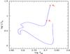 |
Fig. 1 Hertzsprung-Rüssell (HR) diagram showing a 1.3 M⊙ evolutionary track. The red crosses indicate the selected models as described in Sect. 2 and in Table 1. |
Fundamental parameters of the 1.3 M⊙ stellar models.
2. Structures of stellar models and rotation profiles
We consider 1.3 M⊙ models of red giants since this mass is typical of observed red giant stars (Mosser et al. 2010). These models (structure and rotation profile) were evolved from the PMS as described in Paper I.
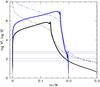 |
Fig. 2 Logarithm of normalized squared Brunt-Väisälä N2 (solid
curve) and (ℓ = 1) Lamb frequencies
|


2.1. Selected models
The first model (M1) lies at the base of the red giant branch (Fig. 1). Its outer convective zone occupies 67% in mass of the outer envelope
and is located at Δm/M = 0.2 above
the H-shell burning. The second model (M2) is farther up on the ascending branch
(Fig. 1). Its outer convective zone occupies 80% of
the outer envelope and is at
Δm/M = 0.015 above the H-shell
burning. Table 1 lists the stellar radius in solar
units, the effective temperature, luminosity in solar units, the central
density ρc, the ratio
 with
with  ,
the radius at the base of the outer convective zone, the radius of maximum nuclear
production rate (both normalized to the stellar radius), the seismic quantities: the large
separation Δν, the g-mode period spacing ΔΠ (in s), the frequency at
maximum power spectrum intensity νmax, the radial order
nmax at νmax.
,
the radius at the base of the outer convective zone, the radius of maximum nuclear
production rate (both normalized to the stellar radius), the seismic quantities: the large
separation Δν, the g-mode period spacing ΔΠ (in s), the frequency at
maximum power spectrum intensity νmax, the radial order
nmax at νmax.
The propagation diagrams (Osaki 1975) for models
M1 and M2 are displayed in Fig. 2. Only the central
part is shown because it plays a major role in determining the properties of the
oscillation modes of red giants (see Sect. 3). The
Brunt-Väisälä (N) and Lamb
(Sℓ) frequencies take their usual
definition, i.e.,  where
Λ = ℓ(ℓ + 1), ℓ is the angular degree
of the mode,
where
Λ = ℓ(ℓ + 1), ℓ is the angular degree
of the mode,  the squared sound
speed, the gravity
g = Gm/r2,
and p,ρ,Γ1 have their usual meaning. Unless otherwise stated,
we consider all squared frequencies
the squared sound
speed, the gravity
g = Gm/r2,
and p,ρ,Γ1 have their usual meaning. Unless otherwise stated,
we consider all squared frequencies  to be
normalized to GM/R3 and
σ2 = ω2/(GM/R3)
(where ω is the mode pulsation in rad/s).
to be
normalized to GM/R3 and
σ2 = ω2/(GM/R3)
(where ω is the mode pulsation in rad/s).
Model M2 is more evolved and more centrally condensed than M1. Accordingly, the inner maximum of the Brunt-Väisälä frequency is higher than for the younger model M1 (Montalbán et al. 2010), and N decreases more sharply. The range of frequency corresponding to the expected excited modes are indicated. They show that the evanescent region between the inner g resonant cavity and the upper p resonant cavity (i.e., between the Brunt-Väisälä and Lamb frequencies) is quite narrow for these modes.
2.2. Rotation profiles
The original rotation profiles obtained for models M1 and M2 from evolution are displayed in Fig. 3. The central regions of the more evolved model M2 rotate much faster than those of M1 (amounting to 181.5 and 260 μHz, respectively). With such high rotation rates, we checked first that the centrifugal acceleration is negligible compared to local gravity in our models (that is, with a relative magnitude of 10-4 at most). We can therefore still safely assume a spherically symmetric equilibrium state. However, the linear approximation is no longer valid due to Coriolis effects when 2Ω/ω is close to unity. This happens in the central regions of the models for the modes we consider. Since we study slowly rotating red giants here, we assumed that some slowing down process has and/or is occurring in real stars that have not yet been included in our models. We therefore artificially decreased the rotation rates stemmed from our evolutionary models so that the first-order approximation for the rotational splittings is valid. The shape of the rotation profile due to slowing down is unknown, we therefore kept it unchanged and investigated whether this can be confirmed or not by confrontation with observations.
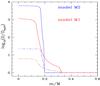 |
Fig. 3 Rotation profiles as a function of the normalized mass. The surface values are Ωsurf/(2π) = 0.154, 0.042 μHz, respectively. Original Ω profiles stemmed from the evolution of the stellar models (red solid curve for model M1 and blue solid curve for model M2). The dot-dashed lines represent the rotation profiles that have been arbitrarily decreased by assuming Ωsurf(Ω/Ωsurf)1/f with f = 3.85 for model M1 (red curve) and f = 2.8 for model M2 (blue curve). |
We therefore decreased the central rotation rates by rescaling the rotation profile stemmed from our evolutionary models, i.e. decreased the central values but kept the same envelope rotation rate. The decrease is set so that the value of the computed rotational splittings agree with observed ones. For instance, for model M1, the initial central rotation, 181.5 μHz, is decreased down to 0.967 μHz. The rotation profiles we used to compute the linear rotational splittings in the following sections are then shown in Fig. 3.
3. Classification of mixed modes
The rotational splittings depend not only on the rotation profile but also on the
eigenfunctions – that is, on the physical nature – of the excited modes. Stellar models of
red giant stars exhibit an outer convective region that is able to efficiently drive modes
stochastically (Samadi et al. 2012). Thus, we
consider only those frequency ranges for our models that span an interval of a few radial
orders below and above nmax (the radial order corresponding to
the frequency at maximum power). We estimate nmax as
nmax = νmax/Δν,
where the frequency at maximum power spectrum νmax and the mean
large separation Δν are given by the usual scaling relations (e.g., Kjeldsen & Bedding 1995)
 \arraycolsep1.75ptwith
Teff, ⊙ = 5777 K and the reference
asymptotic values
νmax, ⊙ = 3106 μHz, and
Δν⊙ = 138.8 μHz defined and calibrated by
Mosser et al. (2013). Indeed, it has been
conjectured by Brown et al. (1991), then shown
observationally by Bedding & Kjeldsen (2003),
that νmax predicts the location of the excited frequency range
of stochastically excited modes well. A physical justification has recently been proposed by
Belkacem et al. (2011). The adiabatic oscillation
frequencies and eigenfunctions for ℓ = 1 modes are computed with the ADIPLS
code (Christensen-Dalsgaard 2008).
\arraycolsep1.75ptwith
Teff, ⊙ = 5777 K and the reference
asymptotic values
νmax, ⊙ = 3106 μHz, and
Δν⊙ = 138.8 μHz defined and calibrated by
Mosser et al. (2013). Indeed, it has been
conjectured by Brown et al. (1991), then shown
observationally by Bedding & Kjeldsen (2003),
that νmax predicts the location of the excited frequency range
of stochastically excited modes well. A physical justification has recently been proposed by
Belkacem et al. (2011). The adiabatic oscillation
frequencies and eigenfunctions for ℓ = 1 modes are computed with the ADIPLS
code (Christensen-Dalsgaard 2008).
Model M1 frequencies of the selected pattern.
Normalized radius of the turning points for selected modes for model M1 frequencies.
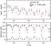 |
Fig. 4 Top: integrated kernel (β I) with β and I given by Eqs. (13) and (8) respectively, (blue dotted line, dots correspond to modes) and mode inertia I (red dotted line, dots correspond to modes) in decimal logarithm for model M1. Black crosses represent the inertia of radial modes. Bottom: rotational splittings (Eq. (11)), in μHz, for ℓ = 1 modes as a function of the normalized frequency ν/Δν for M1 (black dots connected by a dotted line). The magenta open dots connected with the magenta dotted line represents the core contribution to the rotational splittings ⟨ Ω ⟩ coreβcore (Eqs. (15) and (18)). The core contribution to the rotational splittings (Eq. (15)) with ⟨ Ω ⟩ core computed with the horizontal eigenfunction z2 alone is displayed with the blue crosses dotted line. The blue dotted line represents the contribution from the envelope to the rotational splittings ⟨ Ω ⟩ env (β − βcore). The value ⟨ Ω ⟩ core/4π is drawn with the horizontal red dotted line. |
As expected from previous works (e.g., Osaki 1975;
Dziembowski 1977; Dziembowski et al. 2001; Dupret et al.
2009; Montalbán et al. 2010), our red giant
models show many mixed ℓ = 1 modes. For model M1, for instance, the
frequency range of excited modes is expected to be
log 10(σ2) ~ 2−2.8. For modes that are expected
to be excited around νmax (given in Table 2), the corresponding frequencies are much lower than both the
Brunt-Väisälä frequency and the Lamb frequency in the central regions of the models (see
Fig. 2). Therefore, modes with frequencies close to
νmax are trapped in the g resonant cavity, which is located in
the radiative central region. Moreover,  in most of the
envelope so that the modes are also trapped in the p resonant cavity in the convective
envelope (not shown). These cavities’ boundaries are delimited by turning points, i.e. the
radii satisfying
σ2 = N2(r) (g
cavity bounded by x1 and x2) or
in most of the
envelope so that the modes are also trapped in the p resonant cavity in the convective
envelope (not shown). These cavities’ boundaries are delimited by turning points, i.e. the
radii satisfying
σ2 = N2(r) (g
cavity bounded by x1 and x2) or
 (p cavity bounded by
x3 and x4). The location of these
turning points for a list of selected modes are given in Sect. 4.1, Table 3.
(p cavity bounded by
x3 and x4). The location of these
turning points for a list of selected modes are given in Sect. 4.1, Table 3.
To interpret the observed rotational splittings correctly, we need to define a measure of
the g nature of the modes with respect to their p part and classify them accordingly.
Convenient quantities for that purpose are the kinetic energy (Unno et al. 1989) or the mode inertia (Dziembowski et al. 2001), defined as  (5)with
Λ = ℓ(ℓ + 1), and
x = r/R is the
normalized radius. The oscillation quantities entering the above definition are the fluid
vertical and horizontal displacement eigenfunctions ξr and
ξh respectively. For later convenience, we use the following
variables
(5)with
Λ = ℓ(ℓ + 1), and
x = r/R is the
normalized radius. The oscillation quantities entering the above definition are the fluid
vertical and horizontal displacement eigenfunctions ξr and
ξh respectively. For later convenience, we use the following
variables  Using
Eqs. (6) and (7) in (5) leads to
(dropping the subscripts n,ℓ)
Using
Eqs. (6) and (7) in (5) leads to
(dropping the subscripts n,ℓ) 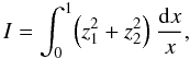 (8)where we have defined
the dimensionless mode inertia I as
I = ℐ/(MR2).
(8)where we have defined
the dimensionless mode inertia I as
I = ℐ/(MR2).
The variation in ℓ = 1 mode inertia with frequency is shown in Figs. 4 and 5 for models M1
and M2. The number of nodes in the g cavity is given by 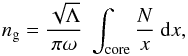 (9)(Unno et al. 1989, and references therein).
Because N2 increases with evolution (see Fig. 2 for M1 and M2), the number of nodes, hence of modes, in a given frequency range increases with the age of the star. This can be seen by comparing Fig. 4 for model M1 and Fig. 5 for model M2. Mixed modes with a g-dominated character have their inertia larger than modes that have their inertia shared between the g and p cavities. These results are in agreement with previous works (e.g., Dupret et al. 2009).
We now define for convenience a measure of the g nature of the mode with the ratio of mode
inertia in the g cavity over the total mode inertia (Deheuvels et al. 2012), i.e., 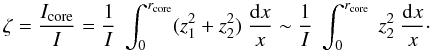 (10)For a mode that is
p-dominated, the inertia is concentrated in the p-cavity and is small due to the low density
in the envelope (ζ ~ 0). Its frequency is mainly determined by the p-cavity
and is therefore half a large separation away from the frequencies of consecutive radial
modes.
(10)For a mode that is
p-dominated, the inertia is concentrated in the p-cavity and is small due to the low density
in the envelope (ζ ~ 0). Its frequency is mainly determined by the p-cavity
and is therefore half a large separation away from the frequencies of consecutive radial
modes.
For a mixed mode where the g character dominates (ζ ~ 1), the mode inertia is strong due to the high density of the central regions where the mode has its maximum amplitude. The frequency of this ℓ = 1 mixed mode differs significantly from that of a ℓ = 1 mode that would be a pure p mode. Its frequency is then closer to that of the closest radial mode. We refer later to such a mode as a g-m mode as in Mosser et al. (2012a).
When the contributions to mode inertia from the core and the envelope are nearly equal, the mode frequencies are less affected by the core and therefore remain closer to the frequencies of pure ℓ = 1 p modes. We refer to such mixed modes as p-m modes (Mosser et al. 2012a). These modes take intermediate values of ζ.
4. Linear rotational splittings
For slow rotation, a first-order perturbation theory provides the following expression for
the rotational splittings (Ledoux 1951; Christensen-Dalsgaard & Berthomieu 1991)
 (11)where Ω is the angular
rotation velocity and the rotational kernel K takes the form
(11)where Ω is the angular
rotation velocity and the rotational kernel K takes the form 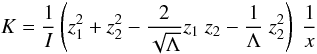 (12)normalized
to the mode inertia I. For later purposes, we also define
(12)normalized
to the mode inertia I. For later purposes, we also define 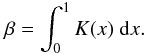 (13)We computed the
rotational splittings according to Eq. (11)
for ℓ = 1 modes and refer to them as numerical rotational splittings later
on. The variations in the rotational splittings with the normalized frequency
ν/Δν are shown for models M1 an M2 in
Figs. 4 and 5.
Also displayed are the variations in both the inertia I and the product
β I (with β and I
respectively given by Eqs. (13) and (8)). They show that the oscillatory variations of
the splittings with frequency are dominated by the nature of the modes since they closely
follow those of mode inertia and of the integrated kernel
β I (see Sect. 4.2).
(13)We computed the
rotational splittings according to Eq. (11)
for ℓ = 1 modes and refer to them as numerical rotational splittings later
on. The variations in the rotational splittings with the normalized frequency
ν/Δν are shown for models M1 an M2 in
Figs. 4 and 5.
Also displayed are the variations in both the inertia I and the product
β I (with β and I
respectively given by Eqs. (13) and (8)). They show that the oscillatory variations of
the splittings with frequency are dominated by the nature of the modes since they closely
follow those of mode inertia and of the integrated kernel
β I (see Sect. 4.2).
It may be useful to the reader to note that models that are located at the same location in the HR diagram (models with the same mass but one with an overshoot of 0.1 pressure scale height and no rotational induced mixing and one without overshoot but with rotational induced mixing) have similar structures. As a consequence, the rotational splitting of any given mode in the range of interest here is the same for both models when computed with the eigenfunctions of the respective models and the same rotation profile.
4.1. Periodic patterns for rotational splittings
It is clear from Figs. 4 and 5 that the variation in the mode inertia and rotational splitting with frequency shows a quasi-periodic pattern, with a period close to the large separation. Each pattern around a radial mode carries roughly the same information about the rotation, at least in the range of observed modes for red giants as found by Mosser et al. (2012a). We note, however, that at higher frequencies, the physical nature of the mixed modes is closer to that of pure p modes and probe the rotation of the surface layers. At lower frequency, the nature of g-m modes is much closer to that of pure g modes and probe the inner rotation better.
The existence of repeated patterns leads us to gather information by folding the power spectrum according to the large separation Δν. The rotational splittings are plotted in Fig. 6 as a function of (ν − ν0)/Δν where ν0 is the closest radial mode to the ℓ = 1 mode of frequency ν. The folding (ν − ν0)/Δν corresponds to the asymptotic folding ν/Δν − (np + ε) as suggested by Mosser et al. (2012b), where np is the radial order of the mode and ε represents some departure from the asymptotic description (Tassoul 1980; Mosser et al. 2012a). This folding is shown for our two models in Fig. 6. We see that all patterns nearly do superpose for each model. Here, ε ~ 1.3−1.4 for model M1 and ε ~ 0 for model M2. A clear correlation exists between the magnitude of the splitting and the g nature of the mixed mode. The minimum, that-is the smallest rotation splittings, corresponds to the p-m modes. The larger rotation splittings that lie on the left- and right-hand sides of this minimum correspond to g-m modes. This agrees with recent observations (Mosser et al. 2012b). In the low-frequency domain, the modes are, for most of them, g-m modes. At higher frequency, they can be either g- or p-m modes (Fig. 6). This is clearly seen when one looks at restricted domains of frequency (corresponding to different color codes in Fig. 6).
We also note that the ratio of the minimum splittings δνmin to the maximum ones δνmax (~0.5 for for model M1 and M2) is only slightly sensitive to rotation. Actually, it only depends on the ratio of the envelope to core rotation, which is small. This is explained in Sect. 6.
 |
Fig. 6 Folded rotational splittings according to (ν − ν0)/Δν for Top: model M1 (blue 9 < ν/Δν < 15; magenta ν/Δν > 15; green ν/Δν < 9) and Bottom: for model M2 (blue 8 < ν/Δν < 14; magenta ν/Δν > 14; green ν/Δν < 8). The splittings are normalized to their maximum values, which are written in the panels. |
4.2. Properties of a periodic pattern
To interpret the behavior of the splittings, we consider a single pattern around a given ℓ = 0 mode with radial-order np = 10 (Table 2) for model M1. There are six modes in the pattern labeled ν1 to ν6 from the lowest to the highest frequency.
4.2.1. Mode inertia I and rotational splittings
The rotational splittings for ν1 to
ν6 are displayed in Fig. 7. The relative contributions
I1/I related to
 , and
I2/I related to
, and
I2/I related to
 , defined as
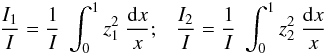 (14)are
displayed in Fig. 7.
(14)are
displayed in Fig. 7.
The contribution of the z1z2
terms to the rotational splittings (Eq. (11)) is negligible in front of in the
envelope and in front of in the
core. Thus, the following conclusions apply for both the mode inertia and the rotational
splittings.
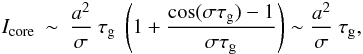
The I1 contribution coincides with the envelope contribution Ienv to a good approximation, while the I2 contribution coincides with the core contribution to a good approximation. The core contribution to inertia, Icore, and the rotational kernel, KΩ, core = ∫coreΩ(x) K(x) dx, are computed between the lower and upper turning points of the g cavity for each mode. The dense core contributes heavily to the total mode inertia I and rotational splittings. The values of the ratio ζ = Icore/I are given in Table 2.
-
The modes with frequencies ν3 and ν4 are g-m modes. For these modes, the contribution of the horizontal displacement z2 (essentially in the core) dominates their inertia (I2/I ~ Icore/I ≈ 1), while the contribution due to the radial displacement z1 (largest in the envelope), I1/I, is negligible. The envelope above the core where the mode is either evanescent or of acoustic type contributes almost nothing to the total mode inertia Ienv/I = 1 − ζ ≪ ζ for such modes. The contribution of the envelope to δν is negligible because the rotation is quite small there.
-
The other modes are p-m modes. The envelope above the core where the mode is either evanescent or acoustic contributes for half for these modes (I1 ~ I2 ~ I/2). They share their inertia almost equally in the core and in the envelope with an almost equal contribution of the horizontal and radial displacements.
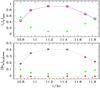 |
Fig. 7 Top: relative inertia contributions
I1/I (green dots
connected dashed line dots correspond to modes) and
I2/I (Eq. (14)) (black), relative contribution
ζ = Icore/I
(magenta dashed line, hexagons correspond to modes). Bottom:
contribution to the rotational splittings for model M1 due to
|

4.2.2. Integrated kernels
The modes are trapped in the same g cavity, so they probe the same inner part of the rotational profile of the model. This can be seen with the behavior of the integrated rotational kernels that are shown in Fig. 8 (left panel). For all modes of the pattern, the integrated rotational kernels increase rapidly from the center.
-
For the g-m modes, the integrated kernels saturate quite rapidly to the maximum value, indicating that the envelope does not significantly contribute. This is the case for ν4 in our studied pattern. The saturated value is obtained long before the upper turning point of the g cavity is reached. This is because the amplitudes of the displacement rapidly become small in the upper part of the g-cavity.
-
The p-m modes, such as ν1 and ν6, have their integrated kernels that saturate less rapidly and to a much lower value than the g-m modes. The corresponding integrated contributions to the splittings are shown in Figs. 7 and 8 (right panel). Since they include the rotation profile, they increase faster than the integrated rotational kernel.
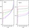 |
Fig. 8 Integrated kernels |


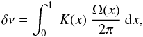
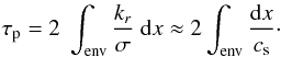
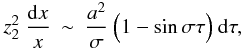
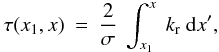
5. Seismic constraint on rotation
For more physical insight into the information carried by rotational splittings, it is
worthwhile emphasizing their dependences. To this end, we decompose the rotational
splittings into two contributions. Given that the inner (radiative) and outer (convective)
cavities have very distinct properties, we write  (15)where
  and
and
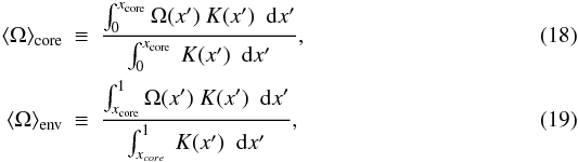 where
K(x) is defined in Eq. (12) and ⟨ Ω ⟩ core is the angular rotation velocity averaged
over the central layers enclosed within a radius
xcore = rcore/R
corresponding to the g resonant cavity. The radius xcore is
taken as the radius of the upper turning point of the g cavity
x2 (see Table 3 for one
pattern). Here, ⟨ Ω ⟩ env is defined as the angular rotation velocity averaged
over the layers above xcore.
where
K(x) is defined in Eq. (12) and ⟨ Ω ⟩ core is the angular rotation velocity averaged
over the central layers enclosed within a radius
xcore = rcore/R
corresponding to the g resonant cavity. The radius xcore is
taken as the radius of the upper turning point of the g cavity
x2 (see Table 3 for one
pattern). Here, ⟨ Ω ⟩ env is defined as the angular rotation velocity averaged
over the layers above xcore.
For the modes we consider in this paper, the evanescent regions above the g resonant cavity and above the p cavity are narrow. Then, the envelope essentially corresponds to the p resonant cavity. The boundary radii are then taken as x3 and x4 (see Table 3). Strictly speaking, the above quantities depend on the frequency mode. However, because of the sharp decrease of the Brunt-Väisälä frequency at the edge of the H shell burning region, the upper turning point of the g cavity is roughly the same for all modes (see Table 3). The modes have a significant amplitude in the g cavity in a region that is quite narrower than the extent of the g cavity and that is independent of the mode (in the frequency regime we consider). This can be seen in Fig. A.1 where the horizontal and radial displacement eigenfunctions are shown for two typical modes of the studied pattern with frequencies listed in Table 2. We can then consider that xcore and the quantity ⟨ Ω ⟩ core are nearly the same for all considered modes.
The radius of the lower turning point, x3, for the p-cavity of
p-m ℓ = 1 modes decreases slightly with increasing frequency of the mode,
while the upper turning point remains approximately the same (see Table 3). In that case, mode inertia depend on the mode. On the
other hand, the mean envelope rotation is nearly that given by the uniform rotation of the
convective zones and remains the same for all modes.  (20)In Fig. 4, the rotational splittings obtained with two
approximations for ⟨ Ω ⟩ core are compared with the exact calculation Eq. (11). The core contribution to the rotational
splittings ⟨ Ω ⟩ coreβcore (Eqs. (15) and (18)) cannot be distinguished from the core contribution to the
rotational splittings (Eq. (15)) with
⟨ Ω ⟩ core computed with the horizontal eigenfunction
z2 alone. The contribution from the envelope to the rotational
splittings ⟨ Ω ⟩ env (β − βcore)
is also represented and is found to be much less for model M2 than for model M1.
(20)In Fig. 4, the rotational splittings obtained with two
approximations for ⟨ Ω ⟩ core are compared with the exact calculation Eq. (11). The core contribution to the rotational
splittings ⟨ Ω ⟩ coreβcore (Eqs. (15) and (18)) cannot be distinguished from the core contribution to the
rotational splittings (Eq. (15)) with
⟨ Ω ⟩ core computed with the horizontal eigenfunction
z2 alone. The contribution from the envelope to the rotational
splittings ⟨ Ω ⟩ env (β − βcore)
is also represented and is found to be much less for model M2 than for model M1.
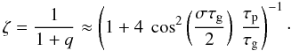
For the g-m modes (i.e. for ζ ~ 1),
βcore ≈ 1/2. The maximum rotational
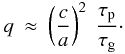
splitting is then given by  (21)The maximum values
of the computed rotational splittings, δνmax,
reach 0.44 and 0.430 μHz for M1 and M2 models, respectively. These values
give rise to a mean core rotation
⟨Ω/2π⟩core = 0.88 μHz
and 0.86 μHz, which are close to, but smaller than the central rotation
for models M1 and M2 respectively (resp. 0.97 and 0.95 μHz). This is
explained by the fact that the rotation decreases sharply in the central regions of our
models and that the major contribution to the rotational splitting is slightly shifted off
the center as are the maximum amplitudes of the horizontal displacement eigenfunctions
(Fig. A.1) and the rotational kernels.
(21)The maximum values
of the computed rotational splittings, δνmax,
reach 0.44 and 0.430 μHz for M1 and M2 models, respectively. These values
give rise to a mean core rotation
⟨Ω/2π⟩core = 0.88 μHz
and 0.86 μHz, which are close to, but smaller than the central rotation
for models M1 and M2 respectively (resp. 0.97 and 0.95 μHz). This is
explained by the fact that the rotation decreases sharply in the central regions of our
models and that the major contribution to the rotational splitting is slightly shifted off
the center as are the maximum amplitudes of the horizontal displacement eigenfunctions
(Fig. A.1) and the rotational kernels.
Moreover, for ℓ = 1 modes, one obtains
βcore ≃ ζ/2 ,
β = 1 − ζ/2, and
βenv = 1 − ζ, to a very good approximation
(Eq. (A.5) in Appendix A.2). Then the linear rotational splitting Eq. (15) is easily rewritten as 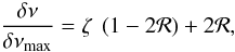 (22)where we have defined the
ratio
(22)where we have defined the
ratio 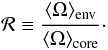 (23)The splittings linearly
increase with ζ. This linear dependence is verified using the numerical
frequencies computed for model M1 and M2 and is shown in Fig. 9.
(23)The splittings linearly
increase with ζ. This linear dependence is verified using the numerical
frequencies computed for model M1 and M2 and is shown in Fig. 9.
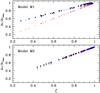 |
Fig. 9 The rotational splitting normalized to its maximum value as a function of ζ (black dots) for model M1 (top) and model M2 (bottom). The red crosses represent the approximation δν/δνmax = ζ as a function of ζ. The blue crosses represent the approximation δν/δνmax = ζ(1 − 2ℛ) + 2ℛ as a function of ζ with R = 0.1785 and using numerical values of ζ. |
We stress that the ratio ℛ imposed by our choice of rotation profile is quite small for
model M2 and the approximation  (24)agrees with the numerical
splitting values.
(24)agrees with the numerical
splitting values.
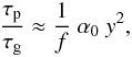
We find that the rotational splittings of p-m modes, as well as g-m modes, are dominated by the central layers for model M2. For the most g-dominated modes, ζ ~ 1, and the rotational splittings in that case directly give half the mean core rotation.
This is not true for less-evolved models such as model M1, for which the approximation Eq. (24) is not sufficient (Fig. 9). The contribution from the envelope layers is not negligible for the rotation profiles we have assumed and the surface rotation must be taken into account as in Eq. (22). This is explained by the p cavity extending quite deep down inside the model where the rotation already shows a sharp gradient toward the center.
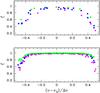 |
Fig. 10 ζ = Icore/I as a function (ν − ν0)/Δν for all l = 1 modes for model M1 (top panel) and for model M2 (bottom panel). ν0 is the frequency of the closest radial mode for the l = 1 mode with frequency ν. For model M1, blue dots correspond to modes with 9 < ν/Δν < 15, magenta dots to modes with ν/Δν > 15, and green dots to modes with ν/Δν < 9). For model M2, blue dots correspond to modes with 8 < ν/Δν < 12, magenta dots to modes with ν/Δν > 12, and green dots to modes with ν/Δν < 8). |
The interest of Eq. (22) is that ζ, as well as δν and δνmax, can be obtained from observations. Mosser et al. (2012b,a) have shown that it is possible to identify the m = 0 modes and their nature (p- or g-dominated mixed). We show here that it is also possible to attribute them a ζ value from the observations. We use as proxy for the measure of the g nature of the mixed mode the distance of the ℓ = 1 mode frequency from that of its companion radial mode: ν − ν0.
Figure 10 shows the ζ values for ℓ = 1 modes as a function of ν − ν0 for models M1 and M2 where ν0 is the frequency of the radial mode closest to ν. The ζ values all follow the same curve. Due to this monotonic dependence, it is possible to estimate the value of ζ from observations (i.e., from the knowledge of ν − ν0). The dispersion of the ζ values about the mean curve in Fig. 10 introduces uncertainties on the induced ζ value. This nevertheless offers a way to derive not only δνmax – hence the mean core rotation – but also the ratio ℛ, hence a measure of the mean rotation gradient from observations.
6. Physical interpretation of the observed splittings
In this section, we show that rotational splittings can be expressed as a function of observables. Indeed, this will further permit us to derive physical properties related to rotation by only using observations (see Sect. 7).
We interpret the two components of the rotational splitting ⟨ Ω ⟩ core and
⟨ Ω ⟩ env physically as the rotation angular velocities averaged over the time
spent in the g and p cavities, respectively. We checked numerically with our stellar models
and numerical frequencies and eigenfunctions that ⟨ Ω ⟩ core and
⟨ Ω ⟩ env are approximated well by mean rotations defined as  (25)The time spent by
the mode is approximately given by
(25)The time spent by
the mode is approximately given by  (26)(Unno et al. 1989, and references therein) where σ is the
normalized frequency of the mode. The radial wave number of the wave normalized to the
stellar radius, kr, is given, in a local asymptotic analysis, by
(26)(Unno et al. 1989, and references therein) where σ is the
normalized frequency of the mode. The radial wave number of the wave normalized to the
stellar radius, kr, is given, in a local asymptotic analysis, by
 (27)(Osaki 1975; Unno et al. 1989)
where N2 and
(27)(Osaki 1975; Unno et al. 1989)
where N2 and  are the
normalized squared Brunt-Väisälä and Lamb frequencies, respectively. As seen below, the
level of approximation is sufficient for our purpose.
are the
normalized squared Brunt-Väisälä and Lamb frequencies, respectively. As seen below, the
level of approximation is sufficient for our purpose.
In the g cavity,  , therefore
 (28)then the time spent in the
resonant g cavity becomes
(28)then the time spent in the
resonant g cavity becomes  (29)This provides the
number of nodes in the g cavity as ng, which is defined as
2πng/σ = τg.
(29)This provides the
number of nodes in the g cavity as ng, which is defined as
2πng/σ = τg.
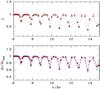 |
Fig. 11 Top: ζ as a function of ν/Δν. Black open symbols: numerical results (Eq. (10)). Red dots: ζ approximated by (Eq. (33)) with χ = 2.5 ycos(π/(ΔΠν)) and y = ν/Δν. Bottom: δν/δνmax as a function of ν/Δν. Black dots: numerical values (Eq. (11)). Red dots: approximate expression for δν/δνmax (Eq. (22)) with ℛ = 0.1785 and ζ given by its numerical values. Blue crosses: δν/δνmax given by Eq. (37) with ℛ = 0.1785 and χ given by Eq. (34). |
Similarly, in the acoustic cavity in the envelope where
 , one can write
 (30)The time
τp and τg are defined in units of
the dynamical time
tdyn = (GM/R3)−1/2.
(30)The time
τp and τg are defined in units of
the dynamical time
tdyn = (GM/R3)−1/2.
The expressions for the mean core (resp. envelope) rotation become  The
theoretical values of
The
theoretical values of  and
and  ,
Eqs. (31) and (32), are computed for both equilibrium models M1
and M2. We find
,
Eqs. (31) and (32), are computed for both equilibrium models M1
and M2. We find  Hz,
Hz,
 Hz,
then
δνmax,th = 0.44 μHz,
ℛ = 0.178 for model M1 and
Hz,
then
δνmax,th = 0.44 μHz,
ℛ = 0.178 for model M1 and 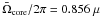 Hz,
Hz,
 Hz,
δνmax,th = 0.428 μHz,
ℛ = 0.05 for model M2 where the subscript th stands for theoretical.
Hz,
δνmax,th = 0.428 μHz,
ℛ = 0.05 for model M2 where the subscript th stands for theoretical.
We then computed the rotational splittings from the approximate expression Eq. (22) using these figures with ζ
computed with the associated eigenfunctions (Eq. (10)). As a result, the theoretical dependence given by Eq. (22) perfectly matches the numerical curve
δν/δνmax
and  ,
,
 .
This can be seen in Fig. 11 for model M1 where one
compares the behavior of the numerical splittings
δν/δνmax
with ν/Δν to the splitting values
obtained by using Eq. (22).
.
This can be seen in Fig. 11 for model M1 where one
compares the behavior of the numerical splittings
δν/δνmax
with ν/Δν to the splitting values
obtained by using Eq. (22).
One can go to a further level of approximation by deriving an approximate expression for
the mode inertia. Appendix A.3 shows that one can
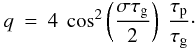
derive an approximate expression for ζ as  (33)where
 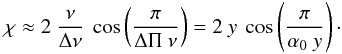 (34)For convenience we have
defined y = ν/Δν and a
dimensionless constant α0 as
(34)For convenience we have
defined y = ν/Δν and a
dimensionless constant α0 as
 (35)with ΔΠ is the period
spacing for g-m modes
(35)with ΔΠ is the period
spacing for g-m modes  (36)For models M1 and M2, we
respectively have α0 = 2.2 × 10⁻³ and
α0 = 6.0 × 10⁻⁴.
(36)For models M1 and M2, we
respectively have α0 = 2.2 × 10⁻³ and
α0 = 6.0 × 10⁻⁴.
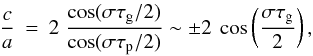
The behavior of the ratio ζ as a function of ν/Δν is computed with Eqs. (33) and (34) and is compared to that of the numerical one in Fig. 11 (top). The cosine term gives rise to the oscillation of ζ, while the decrease in the minimum values of ζ with frequency is driven by the ratio τp/τg. The ratio ζ is computed using Eqs. (33) and (34) where the factor 2 is replaced by a factor 2.5, which fits the numerical results better. This difference is explained by the fact that we took the factor f (Appendix A.3) as equal to unity, while it is in reality smaller. For model M1, the difference between the large separation Δν and the equivalent quantity computed over the p resonant cavity is on the order of f = 0.8. This increases the constant in χ from 2 to 2.24, closer to the adopted 2.5 value. As also mentionned in Appendix A.3, the amplitude ratio Eq. (A.20) is further increased if one takes the effect of the evanescent zone into account between the outer p and inner g resonant cavities of modes. As a consequence, this leads to an increase in the χ term contribution. Actually, some departure from asymptotic is expected for the p part of red giants modes. It is then striking that the numerical results agree that well with Eq. (33).
An expression for the normalized rotational splitting as a function of the observable
y ≡ ν/Δν is then
obtained by combining Eqs. (22) and (33) so that  (37)with χ
given by Eq. (34).
(37)with χ
given by Eq. (34).
The rotational splittings computed with Eqs. (34) and (37) are compared with the numerical values for model M1 in Fig. 11. The behavior of both theoretical and numerical quantities agree quite well. An illustration is provided in Sect. 7 with the red giant star KIC 5356201 (Beck et al. 2012) for which such a procedure has been used.
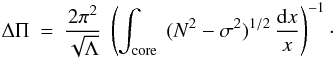
The ratio
δν/δνmax
as a function of
(ν − ν0)/δν
is nearly independent of rotation, in particular when ℛ ≪ 1. Maxima of the
ζ oscillation, ζmax = 1, are obtained for
cos(π/(α0 y)) = 0.
Minima are defined for
cos(π/(α0yn0)) = ± 1,
i.e.,
α0yn0 = 1/n0
(for any integer n0): 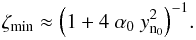 (38)Accordingly, the
contrast η defined as the ratio of minimum to maximum splittings is
obtained from Eq. (37) using Eq. (38) and Eq. (A.23) as
(38)Accordingly, the
contrast η defined as the ratio of minimum to maximum splittings is
obtained from Eq. (37) using Eq. (38) and Eq. (A.23) as 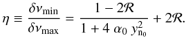 (39)Because
 decreases
with increasing integer n0, the contrast
δνmin/δνmax
increases with frequency for a given rotation profile. This can be seen quite clearly for
model M2 in Fig. 5 for instance.
decreases
with increasing integer n0, the contrast
δνmin/δνmax
increases with frequency for a given rotation profile. This can be seen quite clearly for
model M2 in Fig. 5 for instance.
Typical values of the quantity  for different
types of observed red giants are listed in Table 4,
according to the analysis done by Mosser et al.
(2012b). For simplicity, yn0 is evaluated at
ν = νmax. The first two lines are given for
red giants corresponding to models M1 and M2, respectively, as discussed in the previous
sections. More generally, this quantity decreases from about four at the bottom of the RGB
down to 0.06 for red giants stars located on the highest part of the RGB for which
stochastically oscillations are detected. It amounts to roughly 0.4 for the clump stars.
Note that for the most evolved red giant stars, is quite
small. In that case, the contrast η varies as
for different
types of observed red giants are listed in Table 4,
according to the analysis done by Mosser et al.
(2012b). For simplicity, yn0 is evaluated at
ν = νmax. The first two lines are given for
red giants corresponding to models M1 and M2, respectively, as discussed in the previous
sections. More generally, this quantity decreases from about four at the bottom of the RGB
down to 0.06 for red giants stars located on the highest part of the RGB for which
stochastically oscillations are detected. It amounts to roughly 0.4 for the clump stars.
Note that for the most evolved red giant stars, is quite
small. In that case, the contrast η varies as  (40)and the influence of the
rotation on this contrast throughout ℛ can become negligible.
(40)and the influence of the
rotation on this contrast throughout ℛ can become negligible.
 |
Fig. 12 Top: observed rotational splittings as a function of ν/Δν for the Kepler star KIC 5356201 (Beck et al. 2012). For this star, the mean large separation is Δν = 15.92 μHz while the mean g-mode spaging is ΔΠ = 86.11 s and the maximum rotational splittings is δνmax = 0.405 nHz. Bottom: rotational splittings normalized to δνmax are folded with (ν − ν0)/Δν. |
7. The illustrative case of the red giant KIC 5356201
Differential rotation of the red giant KIC 5356201 observed by Kepler has been analyzed by Beck et al. (2012). Since the inclination of the star has an intermediate value, the three components of the dipole mixed-mode multiplets are clearly visible, which allows precise determination of the rotational splittings. With νmax = 209.7 ± 0.7μHz, Δν = 15.92 ± 0.02 μHz, and a period spacing ΔΠ = 86.2 ± 0.03 s, determined according to the method presented in Mosser et al. (2012b), the star lies at the bottom of the RGB, with a seismically inferred radius of about 4.5 R⊙. The minimum rotational splitting given by Beck et al. (2012) is 0.154 ± 0.003 μHz. The authors also mention that the average contrast between the maximum and minimum value of the splittings is 1.7; the maximum value inferred by Mosser et al. (2012b) is 0.405 ± 0.010 μHz. With such global seismic parameters, one infers that this star is slightly more evolved than model M1 but can be approximately represented by this model.
The observational rotational splittings are displayed as a function of ν/Δν (ν is the frequency of the centroid mode of each identified multiplet) in Fig. 12 (top). The folded splittings are shown in Fig. 12 (bottom). The global behavior of the curve shows the same characteristics as the theoretical equivalent in Fig. 6 for model M1. Only the value of the minimum at (ν − ν0)/Δν is lower than 0.4 (Fig. 12) for the observations compared with 0.59 for model M1 (Fig. 6). The difference is due to different values of the parameters α0 (α0 = 1.37 × 10⁻³ for the Kepler star).
Using the observed values for νmax,Δν and ΔΠ for the star KIC 5356201, we find η = 0.49 (Eq. (39)) when evaluated for the mode with frequency ν/Δν = 13.7(~νmax/Δν). This is close to the observed contrast δν/δνmax = 0.43 evaluated for the same mode. If one corrects η with the factor f mentioned above, taking a typical f = 0.8 as for model M1, one obtains η = 0.45 even closer to the observed value.
In Fig. 13 (top), the observed rotational splittings normalized to their maximum value δνmax are plotted as a function of ζ obtained using Eqs. (33) and (34). The linear dependence of the observed rotational splittings with ζ is clear. One single parameter, 2ℛ, enters the expression for δν/δνmax (Eq. (22)) and can then be estimated to range between 0. and 0.1 from Fig. 13 (top). This indicates that for this star the ratio between the average core rotation and that of the convective envelope is higher than 20. We next compare the theoretical rotational splittings computed using Eqs. (34) and (37) with the observed rotational splittings in Fig. 13 (bottom). The agreement is quite acceptable and validates our theoretical derivations of Sect. 6.
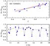 |
Fig. 13 Top: observed rotational splittings as a function of ζ computed with Eqs. (33) and (34) for the Kepler star KIC 5358201 (blue dots). The solid curves are ζ(1 − 2ℛ) + 2ℛ with ℛ = 0 (black) and 2ℛ = 0.1 (red). Bottom: observed rotational splittings (blue filled dots) as a function of ν/Δν. Theoretical rotational splittings computed according to Eqs. (37) and (34) (black open dots connected with a dashed line) with ℛ = 0. |
8. Conclusion
We have investigated the properties of the rotational splittings of the dipole (ℓ = 1) modes of red giant models. The rotational splittings are computed with a first-order perturbation method because we focused on slowly rotating red giant stars. We considered two models in two different H shell-burning evolutionary stages. We find that such modes are either g-m modes (inertia and rotational splittings are fully dominated by the core properties) or p-m modes (inertia is almost equally shared between the core and the envelope). For g-m modes, the rotational splittings are fully dominated by the average core rotation. As the time spent by all considered g-m modes in the core is roughly the same, the resulting mean core rotation corresponds to the rotation in the central layers weighted by the time spent by the modes in the core. For a radiative core, if the rotation decreases sharply from the center, the mean core rotation is a lower limit of the central rotation. For p-m modes, the rotational splittings remain dominated by the core rotation, but the contribution of the envelope is no longer negligible.
We find that the rotational splittings normalized to their maximum value linearly depend on the core contribution of mode inertia. The slope provides the ratio of the average envelope rotation to the core one (ℛ). A one-to-one relation is observed between the mode inertia and the frequency difference between any observed ℓ = 1 mode and the closest radial mode. Because this last quantity is measurable, one can use the simple relation between the core inertia and this frequency difference to determine the core inertia. This knowledge, together with a measure of the rotational splitting, then provides a measure of ℛ.
As a step further in the modeling, we used asymptotic properties to show that the core contribution to mode inertia relative to the total mode inertia depends on the frequency normalized to the large separation through a Lorentzian. This provides a theoretical support for using of a Lorentzian profile for measuring the observed splittings for red giant stars (Mosser et al. 2012a). This also led us to find that the behavior of the rotational splittings of ℓ = 1 modes with the frequency for slowly rotating core red giant stars depends on only three parameters. One is the large separation Δν, the second is the g-mode period spacing ΔΠ, and both can be determined observationally and can therefore again provide a measure of the third one, ℛ.
The contrast between the minimum (δνmin) and maximum (δνmax) values of the splittings can be evaluated at the frequency of maximum power. It only depends on the above three parameters. For a core rotating much faster than the envelope (negligible ℛ), we obtain a relation between (δνmin), (δνmax), Δν and, ΔΠ. This can provide (δνmax) (hence the average core rotation) in cases where the g-m modes have amplitudes that are too small to be detected and only (δνmin) is available.
Based on the theoretical developments above, we find that the Kepler red giant star KIC 53656201 observed by Kepler (Beck et al. 2012) rotates with a rotation in the convective envelope ΩCZ < 0.05 ⟨ Ω ⟩ core ≤ Ω(r = 0) so that the core is rotating more than 20 times faster than the envelope.
The present understanding of the properties of rotational splittings is a contribution to the effort to decipher the effect of slow rotation on red giant star frequency spectra and establish seismic diagnostics on the rotation and transport of angular momentum. For more rapidly rotating red giant stars, nonperturbative methods must be used. This will be the subject of the third paper in this series.
Online material
Appendix A: Properties of eigenfunctions and mode inertia
A.1. Displacement eigenfunctions
 |
Fig. A.1 Displacement eigenfunctions as a function of the normalized radius r/R. In blue the horizontal component to the displacement eigenfunction z2 (Eq. (7)) and in red the radial component to the displacement eigenfunction z1 (Eq. (6)). From top to bottom ℓ = 1 modes 1 and 3 of Table 2. |
The displacement eigenfunctions computed for two modes of the selected pattern (see Table 2) for model M1 are shown as a function of the normalized radius r/R in Fig. A.1. They correspond to the modes with the largest and smallest maximum amplitudes in the pattern. The inner part is dominated by the horizontal displacement z2 and oscillates with a large number of nodes, as is typical of a high-order gravity mode. The largest maximum amplitude corresponds to the most g-dominated mode whereas the smallest maximum amplitudes arise for the p-m modes ν1 and ν6.
The maximum amplitude of z2 occurs deep in the g-cavity, at the same radius for all modes of the pattern. The region of non-negligible amplitude defines the radius of a seismic rotating core which is here found to be independent of the mode (r/R ~ 0.02) and far smaller than the upper turning radius of the inner gravity resonant cavity (x2 ~ 0.08, Table 3)
A.2. Behavior of β and βcore with ζ
For ℓ = 1 modes of red giants, the term
z2z1 in β
(Eq. (13)) plays almost no role
because  in the
core and
in the
core and  in the
envelope (see Fig. A.1). As a result, we have
in the
envelope (see Fig. A.1). As a result, we have
 where
ζ is defined in Eq. (10). The linear dependence of β with ζ is
verified in Fig. A.2. Furthermore, for all
modes,
where
ζ is defined in Eq. (10). The linear dependence of β with ζ is
verified in Fig. A.2. Furthermore, for all
modes,  ,
2z1z2 in the g-cavity (see
Fig. A.1), then
βcore,nl ≈ βcore
where for l = 1 modes, we derive
,
2z1z2 in the g-cavity (see
Fig. A.1), then
βcore,nl ≈ βcore
where for l = 1 modes, we derive  hence
hence
 (A.6)Numerical
values for model M1 confirm that βcore increases linearly
with ζ with a slope 1/2 (Fig. A.2). For g-m modes (ζ ~ 1),
βcore dominates with a nearly constant value of 0.5. P-m
modes correspond to the teeth of the saw-type variation in
βenv and the ratio
βenv/βcore ~ 0.25
(Fig. A.2).
(A.6)Numerical
values for model M1 confirm that βcore increases linearly
with ζ with a slope 1/2 (Fig. A.2). For g-m modes (ζ ~ 1),
βcore dominates with a nearly constant value of 0.5. P-m
modes correspond to the teeth of the saw-type variation in
βenv and the ratio
βenv/βcore ~ 0.25
(Fig. A.2).
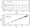 |
Fig. A.2 Top: βenv and βcore as a function of ν/Δν for model M1. Bottom: same as top for the ratio βcore as a function of ζ (black open dots). The approximation β = 1 − (1/2) ζ using the numerical values of ζ is represented with red crosses. |
A.3. An approximate expression for ζ
This section determines an approximate expression of ζ = Icore/I as a function of ν/Δν. The derivation is based on results of an asymptotic method developed by Shibahashi (1979) to which we refer for details (see also Unno et al. 1989).
-
The envelope (~p-propagative cavity) is characterized by
 . Using
Eq. (16.47) from Unno et al., it is straightforward to derive the following
approximate expression
. Using
Eq. (16.47) from Unno et al., it is straightforward to derive the following
approximate expression  (A.7)The
constant c can be determined by the condition
ξr = 1 at the surface.
(A.7)The
constant c can be determined by the condition
ξr = 1 at the surface.
 (A.8)with
 (A.9)where
we have assumed σ2 ≫ N2
in Eq. (27). In the process of
deriving the amplitude of arising
in front of the sinusoidal term in Eq. (A.7), one can neglect in
front of σ2 in the expression for
kr (i.e.
kr ~ σ/cs).
However this is not the case when kr is in the phase
of the sinusoidal term where we keep the expression Eq. (A.9). The inertia in the envelope
can then be approximated as
(A.9)where
we have assumed σ2 ≫ N2
in Eq. (27). In the process of
deriving the amplitude of arising
in front of the sinusoidal term in Eq. (A.7), one can neglect in
front of σ2 in the expression for
kr (i.e.
kr ~ σ/cs).
However this is not the case when kr is in the phase
of the sinusoidal term where we keep the expression Eq. (A.9). The inertia in the envelope
can then be approximated as  where
we have defined
where
we have defined  (A.12)and
the mean large separation is
(A.12)and
the mean large separation is
 (A.13)The
factor f is of order unity and represents the difference
between the integration from x3 and from the center.
We take f = 1 unless specified otherwise. The last equality in
Eq. (A.10) is obtained
assuming στp ≫ 1.
(A.13)The
factor f is of order unity and represents the difference
between the integration from x3 and from the center.
We take f = 1 unless specified otherwise. The last equality in
Eq. (A.10) is obtained
assuming στp ≫ 1. -
The core (~g-propagative cavity) is characterized by
. Again,
the asymptotic results lead to the following expression
 (A.14)where
a is a constant that is determined by the resonant frequency
condition between the p and g cavities, and
(A.14)where
a is a constant that is determined by the resonant frequency
condition between the p and g cavities, and
 (A.15)and
we have used
(A.15)and
we have used 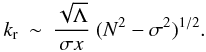 (A.16)Recalling
that στg ≫ 1, therefore the inertia
in the core can be approximated as
(A.16)Recalling
that στg ≫ 1, therefore the inertia
in the core can be approximated as
 (A.17)where
we have defined
(A.17)where
we have defined 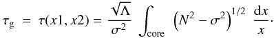 (A.18)
 -
The ratio q ≡ Ienv/Icore is then approximated by
 (A.19)
 -
We obtain the ratio c/a (from Eqs. (16.49) and (16.50) of Unno et al.) as
 (A.20)where
we have used
στp ~ 2npπ.
A exponential term is present in the Unno et al expression with the argument
being an integral over the evanescent region between the p- and g-cavities. As
this region is quite narrow in our models for the considered modes, the
exponential is taken to be 1. Nevertheless the width of the evanescent region
depends on the considered mode, and in some cases, for accurate quantitative
results, it might be necessary to include effects of the evanescent zone with a
finite width.
(A.20)where
we have used
στp ~ 2npπ.
A exponential term is present in the Unno et al expression with the argument
being an integral over the evanescent region between the p- and g-cavities. As
this region is quite narrow in our models for the considered modes, the
exponential is taken to be 1. Nevertheless the width of the evanescent region
depends on the considered mode, and in some cases, for accurate quantitative
results, it might be necessary to include effects of the evanescent zone with a
finite width. -
The ratio q is then eventually approximated by
 (A.21)
 -
For the relative core inertia ζ = Icore/I,
 (A.22)
 -
We now use the approximate expressions Eqs. (A.12) and (A.18) in order to derive for the ratio τp/τg in terms of observable quantities
 (A.23)where
for convenience we have defined
y = ν/Δν,
and
(A.23)where
for convenience we have defined
y = ν/Δν,
and 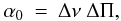 (A.24)with
the period spacing for g modes
(A.24)with
the period spacing for g modes
 (A.25)We
also write
(A.25)We
also write 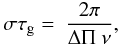 (A.26)so that we
obtain
(A.26)so that we
obtain 
Acknowledgments
JPM acknowledges financial support through a 3-year CDD contract with CNES. R-M.O. is indebted to the “Fédération Wallonie- Bruxelles – Fonds Spéciaux pour la Recherche / Crédit de démarrage – Université de Liège” for financial support. The authors also acknowledge financial support from the French National Research Agency (ANR) for the project ANR-07-BLAN-0226 SIROCO (SeIsmology, ROtation and COnvection with the CoRoT satellite). We also thank the anonymous referee for a careful reading of the manuscript and useful suggestions.
References
- Baglin, A., Auvergne, M., Boisnard, L., et al. 2006, in 36th COSPAR Scientific Assembly, 36, 3749 [Google Scholar]
- Ballot, J., Lignières, F., Reese, D. R., & Rieutord, M. 2010, A&A, 518, A30 [NASA ADS] [CrossRef] [EDP Sciences] [Google Scholar]
- Ballot, J., Lignières, F., Prat, V., Reese, D. R., & Rieutord, M. 2011 [arXiv:1109.6856] [Google Scholar]
- Beck, P. G., Montalban, J., Kallinger, T., et al. 2012, Nature, 481, 55 [NASA ADS] [CrossRef] [Google Scholar]
- Bedding, T. R., & Kjeldsen, H. 2003, PASA, 20, 203 [Google Scholar]
- Bedding, T. R., Mosser, B., Huber, D., et al. 2011, Nature, 471, 608 [NASA ADS] [CrossRef] [PubMed] [Google Scholar]
- Belkacem, K., Goupil, M. J., Dupret, M. A., et al. 2011, A&A, 530, A142 [NASA ADS] [CrossRef] [EDP Sciences] [Google Scholar]
- Borucki, W. J., Koch, D., Basri, G., et al. 2010, Science, 327, 977 [NASA ADS] [CrossRef] [PubMed] [Google Scholar]
- Brown, T. M., Gilliland, R. L., Noyes, R. W., & Ramsey, L. W. 1991, ApJ, 368, 599 [NASA ADS] [CrossRef] [Google Scholar]
- Christensen-Dalsgaard, J. 2008, Ap&SS, 316, 113 [NASA ADS] [CrossRef] [Google Scholar]
- Christensen-Dalsgaard, J., & Berthomieu, G. 1991, Theory of solar oscillations, eds. A. N. Cox, W. C. Livingston, & M. S. Matthews, 401 [Google Scholar]
- De Ridder, J., Barban, C., Baudin, F., et al. 2009, Nature, 459, 398 [Google Scholar]
- Deheuvels, S., García, R. A., Chaplin, W. J., et al. 2012, ApJ, 756, 19 [NASA ADS] [CrossRef] [Google Scholar]
- Dupret, M.-A., Belkacem, K., Samadi, R., et al. 2009, A&A, 506, 57 [NASA ADS] [CrossRef] [EDP Sciences] [Google Scholar]
- Dziembowski, W. A. 1971, Acta Astron., 21, 289 [NASA ADS] [Google Scholar]
- Dziembowski, W. 1977, Acta Astron., 27, 95 [NASA ADS] [Google Scholar]
- Dziembowski, W. A., Gough, D. O., Houdek, G., & Sienkiewicz, R. 2001, MNRAS, 328, 601 [NASA ADS] [CrossRef] [Google Scholar]
- Eggenberger, P., Montalbán, J., & Miglio, A. 2012, A&A, 544, L4 [NASA ADS] [CrossRef] [EDP Sciences] [Google Scholar]
- Hekker, S., Kallinger, T., Baudin, F., et al. 2009, A&A, 506, 465 [NASA ADS] [CrossRef] [EDP Sciences] [Google Scholar]
- Kjeldsen, H., & Bedding, T. R. 1995, A&A, 293, 87 [NASA ADS] [Google Scholar]
- Ledoux, P. 1951, ApJ, 114, 373 [NASA ADS] [CrossRef] [Google Scholar]
- Lignières, F. 2011, in Lect. Notes Phys. (Berlin: Springer Verlag), eds. J.-P. Rozelot, & C. Neiner, 832, 259 [Google Scholar]
- Marques, J. P., Goupil, M. J., Lebreton, Y., et al. 2013, A&A, 549, A74 [NASA ADS] [CrossRef] [EDP Sciences] [Google Scholar]
- Meynet, G., Ekstrom, S., Maeder, A., et al. 2012, Lect. Notes Phys. (in press) [Google Scholar]
- Montalbán, J., Miglio, A., Noels, A., Scuflaire, R., & Ventura, P. 2010, ApJ, 721, L182 [NASA ADS] [CrossRef] [Google Scholar]
- Mosser, B., Belkacem, K., Goupil, M.-J., et al. 2010, A&A, 517, A22 [NASA ADS] [CrossRef] [EDP Sciences] [Google Scholar]
- Mosser, B., Barban, C., Montalbán, J., et al. 2011a, A&A, 532, A86 [NASA ADS] [CrossRef] [EDP Sciences] [Google Scholar]
- Mosser, B., Belkacem, K., Goupil, M. J., et al. 2011b, A&A, 525, L9 [NASA ADS] [CrossRef] [EDP Sciences] [Google Scholar]
- Mosser, B., Goupil, M. J., Belkacem, K., et al. 2012a, A&A, 548, A10 [NASA ADS] [CrossRef] [EDP Sciences] [Google Scholar]
- Mosser, B., Goupil, M. J., Belkacem, K., et al. 2012b, A&A, 540, A143 [NASA ADS] [CrossRef] [EDP Sciences] [Google Scholar]
- Mosser, B., Michel, E., Belkacem, K., et al. 2013, A&A, submitted [Google Scholar]
- Osaki, Y. 1975, PASJ, 27, 237 [NASA ADS] [Google Scholar]
- Ouazzani, R.-M., Dupret, M.-A., & Reese, D. 2012, A&A, 547, A75 [NASA ADS] [CrossRef] [EDP Sciences] [Google Scholar]
- Reese, D., Lignières, F., & Rieutord, M. 2006, A&A, 455, 621 [NASA ADS] [CrossRef] [EDP Sciences] [Google Scholar]
- Samadi, R., Belkacem, K., Dupret, M.-A., et al. 2012, A&A, 543, A120 [NASA ADS] [CrossRef] [EDP Sciences] [Google Scholar]
- Scuflaire, R. 1974, A&A, 36, 107 [NASA ADS] [Google Scholar]
- Shibahashi, H. 1979, PASJ, 31, 87 [NASA ADS] [Google Scholar]
- Tassoul, M. 1980, ApJS, 43, 469 [NASA ADS] [CrossRef] [Google Scholar]
- Unno, W., Osaki, Y., Ando, H., Saio, H., & Shibahashi, H. 1989, Nonradial oscillations of stars (Tokyo: University of Tokyo Press), 2nd edn. [Google Scholar]
All Tables
Normalized radius of the turning points for selected modes for model M1 frequencies.
All Figures
|
Fig. 1 Hertzsprung-Rüssell (HR) diagram showing a 1.3 M⊙ evolutionary track. The red crosses indicate the selected models as described in Sect. 2 and in Table 1. |
| In the text | |
|
Fig. 2 Logarithm of normalized squared Brunt-Väisälä N2 (solid
curve) and (ℓ = 1) Lamb frequencies
|
| In the text | |
|
Fig. 3 Rotation profiles as a function of the normalized mass. The surface values are Ωsurf/(2π) = 0.154, 0.042 μHz, respectively. Original Ω profiles stemmed from the evolution of the stellar models (red solid curve for model M1 and blue solid curve for model M2). The dot-dashed lines represent the rotation profiles that have been arbitrarily decreased by assuming Ωsurf(Ω/Ωsurf)1/f with f = 3.85 for model M1 (red curve) and f = 2.8 for model M2 (blue curve). |
| In the text | |
|
Fig. 4 Top: integrated kernel (β I) with β and I given by Eqs. (13) and (8) respectively, (blue dotted line, dots correspond to modes) and mode inertia I (red dotted line, dots correspond to modes) in decimal logarithm for model M1. Black crosses represent the inertia of radial modes. Bottom: rotational splittings (Eq. (11)), in μHz, for ℓ = 1 modes as a function of the normalized frequency ν/Δν for M1 (black dots connected by a dotted line). The magenta open dots connected with the magenta dotted line represents the core contribution to the rotational splittings ⟨ Ω ⟩ coreβcore (Eqs. (15) and (18)). The core contribution to the rotational splittings (Eq. (15)) with ⟨ Ω ⟩ core computed with the horizontal eigenfunction z2 alone is displayed with the blue crosses dotted line. The blue dotted line represents the contribution from the envelope to the rotational splittings ⟨ Ω ⟩ env (β − βcore). The value ⟨ Ω ⟩ core/4π is drawn with the horizontal red dotted line. |
| In the text | |
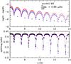 |
Fig. 5 Same as Fig. 4 but for model M2. |
| In the text | |
|
Fig. 6 Folded rotational splittings according to (ν − ν0)/Δν for Top: model M1 (blue 9 < ν/Δν < 15; magenta ν/Δν > 15; green ν/Δν < 9) and Bottom: for model M2 (blue 8 < ν/Δν < 14; magenta ν/Δν > 14; green ν/Δν < 8). The splittings are normalized to their maximum values, which are written in the panels. |
| In the text | |
|
Fig. 7 Top: relative inertia contributions
I1/I (green dots
connected dashed line dots correspond to modes) and
I2/I (Eq. (14)) (black), relative contribution
ζ = Icore/I
(magenta dashed line, hexagons correspond to modes). Bottom:
contribution to the rotational splittings for model M1 due to
|
| In the text | |
|
Fig. 8 Integrated kernels |
| In the text | |
|
Fig. 9 The rotational splitting normalized to its maximum value as a function of ζ (black dots) for model M1 (top) and model M2 (bottom). The red crosses represent the approximation δν/δνmax = ζ as a function of ζ. The blue crosses represent the approximation δν/δνmax = ζ(1 − 2ℛ) + 2ℛ as a function of ζ with R = 0.1785 and using numerical values of ζ. |
| In the text | |
|
Fig. 10 ζ = Icore/I as a function (ν − ν0)/Δν for all l = 1 modes for model M1 (top panel) and for model M2 (bottom panel). ν0 is the frequency of the closest radial mode for the l = 1 mode with frequency ν. For model M1, blue dots correspond to modes with 9 < ν/Δν < 15, magenta dots to modes with ν/Δν > 15, and green dots to modes with ν/Δν < 9). For model M2, blue dots correspond to modes with 8 < ν/Δν < 12, magenta dots to modes with ν/Δν > 12, and green dots to modes with ν/Δν < 8). |
| In the text | |
|
Fig. 11 Top: ζ as a function of ν/Δν. Black open symbols: numerical results (Eq. (10)). Red dots: ζ approximated by (Eq. (33)) with χ = 2.5 ycos(π/(ΔΠν)) and y = ν/Δν. Bottom: δν/δνmax as a function of ν/Δν. Black dots: numerical values (Eq. (11)). Red dots: approximate expression for δν/δνmax (Eq. (22)) with ℛ = 0.1785 and ζ given by its numerical values. Blue crosses: δν/δνmax given by Eq. (37) with ℛ = 0.1785 and χ given by Eq. (34). |
| In the text | |
|
Fig. 12 Top: observed rotational splittings as a function of ν/Δν for the Kepler star KIC 5356201 (Beck et al. 2012). For this star, the mean large separation is Δν = 15.92 μHz while the mean g-mode spaging is ΔΠ = 86.11 s and the maximum rotational splittings is δνmax = 0.405 nHz. Bottom: rotational splittings normalized to δνmax are folded with (ν − ν0)/Δν. |
| In the text | |
|
Fig. 13 Top: observed rotational splittings as a function of ζ computed with Eqs. (33) and (34) for the Kepler star KIC 5358201 (blue dots). The solid curves are ζ(1 − 2ℛ) + 2ℛ with ℛ = 0 (black) and 2ℛ = 0.1 (red). Bottom: observed rotational splittings (blue filled dots) as a function of ν/Δν. Theoretical rotational splittings computed according to Eqs. (37) and (34) (black open dots connected with a dashed line) with ℛ = 0. |
| In the text | |
|
Fig. A.1 Displacement eigenfunctions as a function of the normalized radius r/R. In blue the horizontal component to the displacement eigenfunction z2 (Eq. (7)) and in red the radial component to the displacement eigenfunction z1 (Eq. (6)). From top to bottom ℓ = 1 modes 1 and 3 of Table 2. |
| In the text | |
|
Fig. A.2 Top: βenv and βcore as a function of ν/Δν for model M1. Bottom: same as top for the ratio βcore as a function of ζ (black open dots). The approximation β = 1 − (1/2) ζ using the numerical values of ζ is represented with red crosses. |
| In the text | |
Current usage metrics show cumulative count of Article Views (full-text article views including HTML views, PDF and ePub downloads, according to the available data) and Abstracts Views on Vision4Press platform.
Data correspond to usage on the plateform after 2015. The current usage metrics is available 48-96 hours after online publication and is updated daily on week days.
Initial download of the metrics may take a while.