| Issue |
A&A
Volume 525, January 2011
|
|
|---|---|---|
| Article Number | A139 | |
| Number of page(s) | 11 | |
| Section | Cosmology (including clusters of galaxies) | |
| DOI | https://doi.org/10.1051/0004-6361/201013999 | |
| Published online | 09 December 2010 | |
The galaxy cluster YSZ−LX and YSZ−M relations from the WMAP 5-yr data
1
DSM/Irfu/SPP, CEA/Saclay, 91191
Gif-sur-Yvette Cedex,
France
e-mail: jean-baptiste.melin@cea.fr
2
APC – Université Paris Diderot, 10 rue Alice Domon et Léonie Duquet,
75205
Paris Cedex 13,
France
e-mail: bartlett@apc.univ-paris7.fr
3
APC – CNRS, 10
rue Alice Domon et Léonie Duquet, 75205
Paris Cedex 13,
France
e-mail: delabrouille@apc.univ-paris7.fr
4
DSM/Irfu/SAp, CEA/Saclay, 91191
Gif-sur-Yvette Cedex,
France
e-mail: monique.arnaud@cea.fr; rocco.piffaretti@cea.fr; gabriel.pratt@cea.fr
Received:
6
January
2010
Accepted:
21
October
2010
We use multifrequency matched filters to estimate, in the WMAP 5-year data, the
Sunyaev-Zel’dovich (SZ) fluxes of 893 ROSAT NORAS/REFLEX clusters spanning the luminosity
range
LX,[0.1−2.4] keV = 2 × 1041−3.5 × 1045 erg s-1.
The filters are spatially optimised by using the universal pressure profile recently
obtained from combining XMM-Newton observations of the REXCESSsample and numerical
simulations. Although the clusters are individually only marginally detected, we are able
to firmly measure the SZ signal (>10σ) when
averaging the data in luminosity/mass bins. The comparison between the bin-averaged SZ
signal versus luminosity and X-ray model predictions shows excellent agreement, implying
that there is no deficit in SZ signal strength relative to expectations from the X-ray
properties of clusters. Using the individual cluster SZ flux measurements, we directly
constrain the Y500−LX and
Y500−M500 relations, where
Y500 is the Compton y-parameter integrated
over a sphere of radius r500. The
Y500−M500 relation, derived
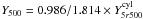
for the first time in such a wide mass range, has a normalisation
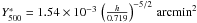
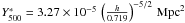
![\hbox{$Y^*_{500} = \left [ 1.60 \pm 0.19 \right ]\times 10^{-3}~{\rm arcmin}^2$}](/articles/aa/full_html/2011/01/aa13999-10/aa13999-10-eq13.png) at
M500 = 3 × 10¹⁴ h-1 M⊙,
in excellent agreement with the X-ray prediction of
1.54 × 10⁻³ arcmin2, and a mass exponent of
α = 1.79 ± 0.17, consistent with the self-similar expectation of
5/3. Constraints on the redshift exponent are weak due to the limited
redshift range of the sample, although they are compatible with self-similar
evolution.
at
M500 = 3 × 10¹⁴ h-1 M⊙,
in excellent agreement with the X-ray prediction of
1.54 × 10⁻³ arcmin2, and a mass exponent of
α = 1.79 ± 0.17, consistent with the self-similar expectation of
5/3. Constraints on the redshift exponent are weak due to the limited
redshift range of the sample, although they are compatible with self-similar
evolution.
Key words: cosmology: observations / galaxies: clusters: general / galaxies: clusters: intracluster medium / cosmic background radiation / X-rays: galaxies: clusters
© ESO, 2010
1. Introduction
Capability to observe the Sunyaev-Zel’dovich (SZ) effect has improved immensely in recent years. Dedicated instruments now produce high resolution images of single objects (e.g. Kitayama et al. 2004; Halverson et al. 2009; Nord et al. 2009) and moderately large samples of high-quality SZ measurements of previously-known clusters (e.g., Mroczkowski et al. 2009; Plagge et al. 2010). In addition, large-scale surveys for clusters using the SZ effect are underway, both from space with the Planck mission (Valenziano et al. 2007; Lamarre et al. 2003) and from the ground with several dedicated telescopes, such as the South Pole Telescope (Carlstrom et al. 2009) leading to the first discoveries of clusters solely through their SZ signal (Staniszewski et al. 2009). These results open the way for a better understanding of the SZ-Mass relation and, ultimately, for cosmological studies with large SZ cluster catalogues.
The SZ effect probes the hot gas in the intracluster medium (ICM). Inverse Compton
scattering of cosmic microwave background (CMB) photons by free electrons in the ICM creates
a unique spectral distortion (Sunyaev & Zeldovich
1970, 1972) seen as a frequency-dependent
change in the CMB surface brightness in the direction of galaxy clusters that can be written
as  ,
where jν is a universal function of the
dimensionless frequency
x = hν/kTcmb.
The Compton y-parameter is given by the integral of the electron pressure
along the line-of-sight in the direction
,
where jν is a universal function of the
dimensionless frequency
x = hν/kTcmb.
The Compton y-parameter is given by the integral of the electron pressure
along the line-of-sight in the direction  ,
,
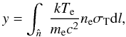 (1)where
σT is the Thomson cross section.
(1)where
σT is the Thomson cross section.
Most notably, the integrated SZ flux from a cluster directly measures the total thermal
energy of the gas. Expressing this flux in terms of the integrated Compton
y-parameter YSZ – defined by
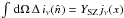 – we see that
YSZ ∝ ∫ dΩ dlneTe ∝ ∫ neTedV.
For this reason, we expect YSZ to closely correlate with total
cluster mass, M, and to provide a low-scatter mass proxy.
– we see that
YSZ ∝ ∫ dΩ dlneTe ∝ ∫ neTedV.
For this reason, we expect YSZ to closely correlate with total
cluster mass, M, and to provide a low-scatter mass proxy.
This expectation, borne out by both numerical simulations (e.g., da Silva et al. 2004; Motl et al. 2005; Kravtsov et al. 2006) and indirectly from X-ray observations using YX, the product of the gas mass and mean temperature (Nagai et al. 2007; Arnaud et al. 2007; Vikhlinin et al. 2009), strongly motivates the use of SZ cluster surveys as cosmological probes. Theory predicts the cluster abundance and its evolution – the mass function – in terms of M and the cosmological parameters. With a good mass proxy, we can measure the mass function and its evolution and hence constrain the cosmological model, including the properties of dark energy. In this context the relationship between the integrated SZ flux and total mass, YSZ−M, is fundamental as the required link between theory and observation. Unfortunately, despite its importance, we are only beginning to observationally constrain the relation (Bonamente et al. 2008; Marrone et al. 2009).
Several authors have extracted the cluster SZ signal from WMAP data (Bennett et al. 2003; Hinshaw et al. 2007, 2009). However, the latter are not ideal for SZ observations: the instrument having been designed to measure primary CMB anisotropies on scales larger than galaxy clusters, the spatial resolution and sensitivity of the sky maps render cluster detection difficult. Nevertheless, these authors extracted the cluster SZ signal by either cross-correlating with the general galaxy distribution (Fosalba et al. 2003; Myers et al. 2004; Hernández-Monteagudo et al. 2004, 2006) or “stacking” existing cluster catalogues in the optical or X-ray (Lieu et al. 2006; Afshordi et al. 2007; Atrio-Barandela et al. 2008; Bielby & Shanks 2007; Diego & Partridge 2009). These analyses indicate that an isothermal β-model is not a good description of the SZ profile, and some suggest that the SZ signal strength is lower than expected from the X-ray properties of the clusters (Lieu et al. 2006; Bielby & Shanks 2007).
Recent in-depth X-ray studies of the ICM pressure profile demonstrate regularity in shape and simple scaling with cluster mass. Combining these observations with numerical simulations leads to a universal pressure profile (Nagai et al. 2007; Arnaud et al. 2010) that is best fit by a modified NFW profile. The isothermal β-model, on the other hand, does not provide an adequate fit. From this newly determined X-ray pressure profile, we can infer the expected SZ profile, y(r), and the YSZ−M relation at low redshift (Arnaud et al. 2010).
It is in light of this recent progress from X-ray observations that we present a new analysis of the SZ effect in WMAP with the aim of constraining the SZ scaling laws. We build a multifrequency matched filter (Herranz et al. 2002; Melin et al. 2006) based on the known spectral shape of the thermal SZ effect and the shape of the universal pressure profile of Arnaud et al. (2010). This profile was derived from REXCESS (Böhringer et al. 2007), a sample expressly designed to measure the structural and scaling properties of the local X-ray cluster population by means of an unbiased, representative sampling in luminosity. Using the multifrequency matched filter, we search for the SZ effect in WMAP from a catalogue of 893 clusters detected by ROSAT, maximising the signal-to-noise by adapting the filter scale to the expected characteristic size of each cluster. The size is estimated through the luminosity-mass relation derived from the REXCESS sample by Pratt et al. (2009).
We then use our SZ measurements to directly determine the YSZ−LX and YSZ−M relations and compare to expectations based on the universal X-ray pressure profile. As compared to the previous analyses of Bonamente et al. (2008) and Marrone et al. (2009), the large number of systems in our WMAP/ROSAT sample allows us to constrain both the normalisation and slope of the YSZ−LX and YSZ−M relations over a wider mass range and in the larger aperture of r500. In addition, the analysis is based on a more realistic pressure profile than in these analyses, which were based on an isothermal β-model. Besides providing a direct constraint on these relations, the good agreement with X-ray predictions implies that there is in fact no deficit in SZ signal strength relative to expectations from the X-ray properties of these clusters.
The discussion proceeds as follows. We first present the WMAP 5-year data and the ROSAT cluster sample used, a combination of the REFLEX and NORAS catalogues. We then present the SZ model based on the X-ray-measured pressure profile (Sect. 3). In Sect. 4, we discuss our SZ measurements, after first describing how we extract the signal using the matched filter. Section 5 details the error budget. We compare our measured scaling laws to the X-ray predictions in Sects. 6 and 7 and then conclude in Sect. 8. Finally, we collect useful SZ definitions and unit conversions in the Appendices.
Throughout this paper, we use the WMAP5-only cosmological parameters set as our “fiducial
cosmology”, i.e. h = 0.719, ΩM = 0.26, ΩΛ = 0.74,
where h is the Hubble parameter at redshift z = 0 in
units of 100 km s-1/Mpc. We note
h70 = h/0.7 and
E(z) is the Hubble parameter at
redshift z normalised to its present value.
M500 is defined as the mass within the radius
r500 at which the mean mass density is 500 times the critical
density, ρcrit(z), of the universe at the
cluster redshift: 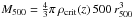 .
.
2. The WMAP-5yr data and the NORAS/REFLEX cluster sample
2.1. The WMAP-5 yr data
We work with the WMAP full resolution coadded five year sky temperature maps at each frequency channel (downloaded from the LAMBDA archive1). There are five full sky maps corresponding to frequencies 23, 33, 41, 61, 94 GHz (bands K, Ka,Q,V,W respectively). The corresponding beam full widths at half maximum are approximately 52.8, 39.6, 30.6 21.0 and 13.2 arcmins. The maps are originally at HEALPix2 resolution nside = 512 (pixel = 6.87 arcmin). Although this is reasonably adequate to sample WMAP data, it is not adapted to the multifrequency matched filter algorithm we use to extract the cluster fluxes. We oversample the original data, to obtain nside = 2048 maps, by zero-padding in harmonic space. In detail, this is performed by computing the harmonic transform of the original maps, and then performing the back transform towards a map with nside = 2048, with a maximum value of ℓ of ℓmax = 750, 850, 1100, 1500, 2000 for the K,Ka,Q,V,W bands respectively. The upgraded maps are smooth and do not show pixel edges as we would have obtained using the HEALPix upgrading software, based on the tree structure of the HEALPix pixelisation scheme. This smooth upgrading scheme is important as the high spatial frequency content induced by pixel edges would have been amplified through the multifrequency matched filters implemented in harmonic space.
In practice, the multifrequency matched filters are implemented locally on small, flat patches (gnomonic projection on tangential maps), which permits adaptation of the filter to the local conditions of noise and foreground contamination. We divide the sphere into 504 square tangential overlapping patches (100 deg2 each, pixel = 1.72 arcmin). All of the following analysis is done on these sky patches.
The implementation of the matched filter requires knowledge of the WMAP beams. In this work, we assume symmetric beams, for which the transfer function bℓ is computed, in each frequency channel, from the noise-weighted average of the transfer functions of individual differential assemblies (a similar approach was used in Delabrouille et al. 2009).
2.2. The NORAS/REFLEX cluster sample and derived X-ray properties
We construct our cluster sample from the largest published X-ray catalogues: NORAS (Böhringer et al. 2000) and REFLEX (Böhringer et al. 2004), both constructed from the ROSAT All-Sky Survey. We merge the cluster lists given in Tables 1, 6 and 8 from Böhringer et al. (2000) and Table 6 from Böhringer et al. (2004) and since the luminosities of the NORAS clusters are given in a standard cold dark matter (SCDM) cosmology (h = 0.5, ΩM = 1), we converted them to the WMAP5 cosmology. We also convert the luminosities of REFLEX clusters from the basic ΛCDM cosmology (h = 0.7, ΩM = 0.3, ΩΛ = 0.7) to the more precise WMAP5 cosmology. Removing clusters appearing in both catalogues leaves 921 objects, of which 893 have measured redshifts. We use these 893 clusters in the analysis detailed in the next section.
The NORAS/REFLEX luminosities LX, measured in the soft
[0.1–2.4] keV energy band, are given within various apertures depending on the
cluster. We convert the luminosities LX to
L500, the luminosities within
r500, using an iterative scheme. This scheme is based on the
mean electron density profile of the REXCESS cluster sample (Croston et al. 2008), which allows conversion of the luminosity between
various apertures, and the REXCESS
L500−M500 relation (Pratt et al. 2009), which implicitly relates
r500 and L500. The procedure
thus simultaneously yields an estimate of the cluster mass,
M500, and the corresponding angular extent
θ500 = r500/Dang(z),
where Dang(z) is the angular distance at
redshift z. In the following we consider values derived from relations
both corrected and uncorrected for Malmquist bias. The relations are described by the
following power law models3: 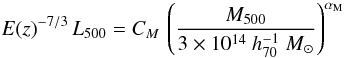 (2)where
the normalisation CM, the exponent
αM and the dispersion (nearly constant with mass) are given
in Table 1. The
L500−M500 relation was derived
in the mass range
[1014−1015] M⊙. These limits
are shown in Fig. 1. Note that we assume the relation
is valid for lower masses.
(2)where
the normalisation CM, the exponent
αM and the dispersion (nearly constant with mass) are given
in Table 1. The
L500−M500 relation was derived
in the mass range
[1014−1015] M⊙. These limits
are shown in Fig. 1. Note that we assume the relation
is valid for lower masses.
Values for the parameters of the LX − M relation derived from REXCESS data (Pratt et al. 2009; Arnaud et al. 2010).
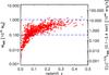 |
Fig. 1 Inferred masses for the 893 NORAS/REFLEX clusters as a function of redshift. The cluster sample is flux limited. The right vertical axis gives the corresponding X-ray luminosities scaled by E(z)−7/3. The dashed blue lines delineate the mass range over which the L500−M500 relation from Pratt et al. (2009) was derived. |
3. The cluster SZ model
In this section we describe the cluster SZ model, based on X-ray observations of the REXCESS sample combined with numerical simulations, as presented in Arnaud et al. (2010). We use the standard self-similar model presented in their Appendix B. Given a cluster mass M500 and redshift z, the model predicts the electronic pressure profile. This gives both the SZ profile shape and Y500, the SZ flux integrated in a sphere of radius r500.
3.1. Cluster shape
The dimensionless universal pressure profile is taken from Eqs. (B1) and (B2) of Arnaud et al. (2010):  (3)where
x = r/rs
with
rs = r500/c500
and c500 = 1.156, α = 1.0620,
β = 5.4807, γ = 0.3292 and with
P500 defined in Eq. (4) below.
(3)where
x = r/rs
with
rs = r500/c500
and c500 = 1.156, α = 1.0620,
β = 5.4807, γ = 0.3292 and with
P500 defined in Eq. (4) below.
This profile shape is used to optimise the SZ signal detection. As described below in Sect. 4, we extract the YSZ flux from WMAP data for each ROSAT system fixing c500, α, β, γ to the above values, but leaving the normalisation free.
3.2. Normalisation
The model allows us to compute the physical pressure profile as a function of mass
and z, thus the
YSZ−M500 relation by
integration of P(r) to r500.
For the shape parameters given above, the normalisation parameter
 and the self-similar
definition of P500 (Arnaud
et al. 2010, Eq. (5) and Eq. (B2)),
and the self-similar
definition of P500 (Arnaud
et al. 2010, Eq. (5) and Eq. (B2)),  (4)one obtains:
![\begin{eqnarray} \label{ym_ss_rel} Y_{500}~[{\rm arcmin}^2] &=& Y^*_{500} \, \left({M_{500} \over 3\times 10^{14}\,h^{-1}~M_\odot} \right)^{5/3} \nonumber\\ &\quad \times & E(z)^{2/3} \, \left( {D_{\rm ang} (z) \over 500~{\rm Mpc}} \right )^{-2}, \end{eqnarray}](/articles/aa/full_html/2011/01/aa13999-10/aa13999-10-eq93.png) (5)where
(5)where
 . Equivalently,
one can write:
. Equivalently,
one can write: ![\begin{equation} Y_{500} \, \, [{\rm Mpc}^2] = Y^*_{500} \; \left ({M_{500} \over 3\times10^{14}\,h^{-1}~M_\odot} \right )^{5/3} \; E(z)^{2/3} \end{equation}](/articles/aa/full_html/2011/01/aa13999-10/aa13999-10-eq95.png) (6)where
(6)where
 . Details of unit
conversions are given in Appendix B. The mass
dependence (
. Details of unit
conversions are given in Appendix B. The mass
dependence ( )
and the redshift dependence
(E(z)2/3) of the
relation are self-similar by construction. This model is used to predict the
Y500 value for each cluster. These predictions are compared
to the WMAP-measured values in Figs. 3–6.
)
and the redshift dependence
(E(z)2/3) of the
relation are self-similar by construction. This model is used to predict the
Y500 value for each cluster. These predictions are compared
to the WMAP-measured values in Figs. 3–6.
4. Extraction of the SZ flux
4.1. Multifrequency matched filters
We use multifrequency matched filters to estimate cluster fluxes from the WMAP frequency maps. By incorporating prior knowledge of the cluster signal, i.e., its spatial and spectral characteristics, the method maximally enhances the signal-to-noise of a SZ cluster source by optimally filtering the data. The universal profile shape described in Sect. 3 is assumed, and we evaluate the effects of uncertainty in this profile as outlined in Sect. 5 where we discuss our overall error budget. We fix the position and the characteristic radius θs of each cluster and estimate only its flux. The position is taken from the NORAS/REFLEX catalogue and θs = θ500/c500 with θ500 derived from X-ray data as described in Sect. 2.2. Below, we recall the main features of the multifrequency matched filters. More details can be found in Herranz et al. (2002) or Melin et al. (2006).
Consider a cluster with known radius θs and unknown central
y-value yo positioned at a known point
xo on the sky. The region is covered by the five WMAP maps
Mi(x) at frequencies
νi = 23, 33, 41, 61, 94 GHz
(i = 1,...,5). We
arrange the survey maps into a column vector
M(x) whose ith component
is the map at frequency νi. The maps contain
the cluster SZ signal plus noise:  (7)where
N is the noise vector (whose components are noise maps
at the different observation frequencies) and
jν is a
vector with components given by the SZ spectral function
jν evaluated at each frequency. Noise in
this context refers to both instrumental noise as well as all signals other than the
cluster thermal SZ effect; it thus also comprises astrophysical foregrounds, for example,
the primary CMB anisotropy, diffuse Galactic emission and extragalactic point sources.
Tθs(x − xo)
is the SZ template, taking into account the WMAP beam, at projected distance
(x − xo) from the cluster centre,
normalised to a central value of unity before convolution. It is computed by integrating
along the line-of-sight and normalising the universal pressure profile (Eq. (3)). The profile is truncated at
5 × r500 (i.e. beyond the virial radius) so that what is
actually measured is the flux within a cylinder of aperture radius
5 × r500.
(7)where
N is the noise vector (whose components are noise maps
at the different observation frequencies) and
jν is a
vector with components given by the SZ spectral function
jν evaluated at each frequency. Noise in
this context refers to both instrumental noise as well as all signals other than the
cluster thermal SZ effect; it thus also comprises astrophysical foregrounds, for example,
the primary CMB anisotropy, diffuse Galactic emission and extragalactic point sources.
Tθs(x − xo)
is the SZ template, taking into account the WMAP beam, at projected distance
(x − xo) from the cluster centre,
normalised to a central value of unity before convolution. It is computed by integrating
along the line-of-sight and normalising the universal pressure profile (Eq. (3)). The profile is truncated at
5 × r500 (i.e. beyond the virial radius) so that what is
actually measured is the flux within a cylinder of aperture radius
5 × r500.
X-ray observations are typically well-constrained out to r500. Our decision to integrate out to 5 × r500 is motivated by the fact that for the majority of clusters the radius r500 is of order the Healpix pixel size (nside = 512, pixel = 6.87 arcmin). Integrating only out to r500 would have required taking into account that only a fraction of the flux of some pixels contributes to the true SZ flux in a cylinder of aperture radius r500. We thus obtain the total SZ flux of each cluster by integrating out to 5 × r500, and then convert this to the value in a sphere of radius r500 for direct comparison with the X-ray prediction.
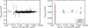 |
Fig. 2 Left: estimated SZ flux from a cylinder of aperture radius
5 × r500 ( |
The multifrequency matched filters
Ψθs(x)
return a minimum variance unbiased estimate,  ,
of yo when centered on the cluster:
,
of yo when centered on the cluster: 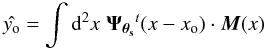 (8)where superscript
t indicates a transpose (with complex conjugation when necessary). This
is just a linear combination of the maps, each convolved with its frequency-specific
filter (Ψθs)i. The
result expressed in Fourier space is:
(8)where superscript
t indicates a transpose (with complex conjugation when necessary). This
is just a linear combination of the maps, each convolved with its frequency-specific
filter (Ψθs)i. The
result expressed in Fourier space is:
 (9)where
 ![\begin{eqnarray} \vec{\Ft}({k}) & \equiv & \vec{\jnu} \Ts({k})\\ \label{eq:sigt} \sigt & \equiv & \left[\int {\rm d}^2k\; \vec{\Ft}^t( {k})\cdot \vec{P}^{-1} \cdot \vec{\Ft}( {k})\right]^{-1/2} \end{eqnarray}](/articles/aa/full_html/2011/01/aa13999-10/aa13999-10-eq125.png) with
P(k) being the noise power spectrum, a
matrix in frequency space with components Pij
defined by
with
P(k) being the noise power spectrum, a
matrix in frequency space with components Pij
defined by  . The quantity
σθs gives the total noise
variance through the filter, corresponding to the statistical errors quoted in this paper.
The other uncertainties are estimated separately as described in Sect. 5.1. The noise power spectrum
P(k) is directly estimated from the maps:
since the SZ signal is subdominant at each frequency, we assume
N(x) ≈ M(x)
to do this calculation. We undertake the Fourier transform of the maps and average their
cross-spectra in annuli with width Δl = 180.
. The quantity
σθs gives the total noise
variance through the filter, corresponding to the statistical errors quoted in this paper.
The other uncertainties are estimated separately as described in Sect. 5.1. The noise power spectrum
P(k) is directly estimated from the maps:
since the SZ signal is subdominant at each frequency, we assume
N(x) ≈ M(x)
to do this calculation. We undertake the Fourier transform of the maps and average their
cross-spectra in annuli with width Δl = 180.
4.2. Measurements of the SZ flux
The derived total WMAP flux from a cylinder of aperture radius
5 × r500 ( ) for the 893
individual NORAS/REFLEX clusters is shown as a function of the measured X-ray luminosity
L500 in the left-hand panel of Fig. 2. The clusters are barely detected individually. The average
signal-to-noise ratio (S/N) of the
total population is 0.26 and only 29 clusters are detected at
S/N > 2,
the highest detection being at 4.2. However, one can distinguish the deviation towards
positive flux at the very high luminosity end.
) for the 893
individual NORAS/REFLEX clusters is shown as a function of the measured X-ray luminosity
L500 in the left-hand panel of Fig. 2. The clusters are barely detected individually. The average
signal-to-noise ratio (S/N) of the
total population is 0.26 and only 29 clusters are detected at
S/N > 2,
the highest detection being at 4.2. However, one can distinguish the deviation towards
positive flux at the very high luminosity end.
In the right-hand panel of Fig. 2, we average the
893 measurements in four logarithmically-spaced luminosity bins (red diamonds plotted at
bin center). The number of clusters are 7, 150, 657, 79 from the lowest to the highest
luminosity bin. Here and in the following, the bin average is defined as the weighted mean
of the SZ flux in the bin (weight of  ). The thick
error bars correspond to the statistical uncertainties on the WMAP data only, while the
thin bar gives the total errors as discussed in Sect. 5.1. The SZ signal is clearly detected in the two highest luminosity bins (at
6.0 and 5.4σ, respectively). As a demonstrative check, we have undertaken
the analysis a second time using random cluster positions. The result is shown by the
green triangles in Fig. 2 and is consistent with no
SZ signal, as expected.
). The thick
error bars correspond to the statistical uncertainties on the WMAP data only, while the
thin bar gives the total errors as discussed in Sect. 5.1. The SZ signal is clearly detected in the two highest luminosity bins (at
6.0 and 5.4σ, respectively). As a demonstrative check, we have undertaken
the analysis a second time using random cluster positions. The result is shown by the
green triangles in Fig. 2 and is consistent with no
SZ signal, as expected.
In the following sections, we study both the relation between the SZ signal and the X-ray
luminosity and that with the mass M500. We consider
Y500, the SZ flux from a sphere of radius
r500, converting the measured
into
Y500 as described in Appendix A. This allows a more direct comparison with the model derived from
X-ray observations (Sect. 3). Before presenting the
results, we first discuss the overall error budget.
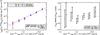 |
Fig. 3 Left: bin averaged SZ flux from a sphere of radius r500 (Y500) as a function of X-ray luminosity in a aperture of r500 (L500). The WMAP data (red diamonds and crosses), the SZ cluster signal expected from the X-ray based model (blue stars) and the combination of the Y500−M500 and L500−M500 relations (dash and dotted dashed lines) are given for two analyses, using respectively the intrinsic L500−M500 and the REXCESS L500−M500 relations. As expected, the data points do not change significantly from one case to the other showing that the Y500-L500 relation is rather insensitive to the finer details of the underlying L500−M500 relation. Right: ratio of data points to model for the two analysis. The points for the analysis undertaken with the intrinsic L500−M500 are shifted to lower luminosities by 20% for clarity. |
5. Overall error budget
5.1. Error due to dispersion in X-ray properties
The error σθs on Y500 given by the multifrequency matched filter only includes the statistical SZ measurement error, due to the instrument (beam, noise) and to the astrophysical contaminants (primary CMB, Galaxy, point sources). However, we must also take into account: 1) uncertainties on the cluster mass estimation from the X-ray luminosities via the L500−M500 relation, 2) uncertainties on the cluster profile parameters. These are sources of error on individual Y500 estimates (actual parameters for each individual cluster may deviate somewhat from the average cluster model). These deviations from the mean, however, induce additional random uncertainties on statistical quantities derived from Y500, i.e. bin averaged Y500 values and the Y500−L500 scaling relation parameters. Their impact on the Y500−M500 relation, which depends directly on the M500 estimates, is also an additional random uncertainty.
The uncertainty on M500 is dominated by the intrinsic dispersion in the L500−M500 relation. Its effect is estimated by a Monte Carlo (MC) analysis of 100 realisations. We use the dispersion at z = 0 as estimated by Pratt et al. (2009), given in Table 1. For each realisation, we draw a random mass log M500 for each cluster from a Gaussian distribution with mean given by the L500−M500 relation and standard deviation σlog L−log M/αM. We then redo the full analysis (up to the fitting of the YSZ scaling relations) with the new values of M500 (thus θs).
The second uncertainty is due to the observed dispersion in the cluster profile shape, which depends on radius as shown in Arnaud et al. (2010, σlog P ~ 0.10. Using new 100 MC realisations, we estimate this error by drawing a cluster profile in the log-log plane from a Gaussian distribution with mean given by Eq. (3) and standard deviation depending on the cluster radius as shown in the lower panel of Fig. 2 in Arnaud et al. (2010).
The total error on Y500 and on the scaling law parameters is calculated from the quadratic sum of the standard deviation of both the above MC realisations and the error due to the SZ measurement uncertainty.
5.2. The Malmquist bias
The NORAS/REFLEX sample is flux limited and is thus subject to the Malmquist bias (MB). This is a source of systematic error. Ideally we should use a L500−M500 relation which takes into account the specific bias of the sample, i.e. computed from the true L500−M500 relation, with dispersion and bias according to each survey selection function. We have an estimate of the true, ie MB corrected, L500−M500 relation, from the published analysis of REXCESS data (Table 1). However, while the REFLEX selection function is known and available, this is not the case for the NORAS sample. This means that we cannot perform a fully consistent analysis. In order to estimate the impact of the Malmquist Bias we thus present, in the following, results for two cases.
In the first case, we use the published L500−M500 relation derived directly from the REXCESS data, i.e. not corrected for the REXCESS MB (hereafter the REXCESS L500−M500 relation). Note that the REXCESS is a sub-sample of REFLEX. Using this relation should result in correct masses if the Malmquist bias for the NORAS/REFLEX sample is the same as that for the REXCESS. The Y500−M500 relation derived in this case would also be correct and could be consistently compared with the X-ray predicted relation. We recall that this relation was derived from pressure and mass measurements that are not sensitive to the Malmquist bias. However L500 would remain uncorrected so that the Y500−L500 relation derived in this case should be viewed as a relation uncorrected for the Malmquist bias. In the second case, we use the MB corrected L500−M500 relation (hereafter the intrinsic L500−M500 relation). This reduces to assuming that the Malmquist bias is negligible for the NORAS/REFLEX sample. The comparison of the two analyses provides an estimate of the direction and amplitude of the effect of the Malmquist bias on our results. The REXCESS L500−M500 relation is expected to be closer to the L500−M500 relation for the NORAS/REFLEX sample than the intrinsic relation. The discussions and figures correspond to the results obtained when using the former, unless explicitly specified.
Fitted parameters for the observed YSZ–L500 relation.
The choice of the L500−M500
relation has an effect both on the estimated L500,
M500 and Y500 values and on the
expectation for the SZ signal from the NORAS/REFLEX clusters. However, for a cluster of
given luminosity measured a given aperture, L500 depends
weakly on the exact value of r500 due to the steep drop of
X-ray emission with radius. As a result, and although L500 and
M500 (or equivalently r500) are
determined jointly in the iterative procedure described in Sect. 2.2, changing the underlying
L500−M500 relation mostly
impacts the M500 estimate: L500 is
essentially unchanged (median difference of ~0.8%) and the difference in
M500 simply reflects the difference between the relations at
fixed luminosity. This has an impact on the measured Y500 via
the value of r500 (the profile shape being fixed) but the
effect is also small (<1%). This is due to the rapidly
converging nature of the YSZ flux (see Fig. 11 of Arnaud et al. 2010). On the other hand, all results that
depend directly on M500, namely the derived
Y500−M500 relation or the
model value for each cluster, that varies as  (Eq. (5)), depend sensitively on the
L500−M500 relation.
M500 derived from the intrinsic relation is higher, an
effect increasing with decreasing cluster luminosity (see Fig. B2 of Pratt et al. 2009).
(Eq. (5)), depend sensitively on the
L500−M500 relation.
M500 derived from the intrinsic relation is higher, an
effect increasing with decreasing cluster luminosity (see Fig. B2 of Pratt et al. 2009).
5.3. Other possible sources of uncertainty
The analysis presented in this paper has been performed on the entire NORAS/REFLEX cluster sample without removal of clusters hosting radio point sources. To investigate the impact of the point sources on our result, we have cross-correlated the NVSS (Condon et al. 1998) and SUMMS (Mauch et al. 2003) catalogues with our cluster catalogue. We conservatively removed from the analysis all the clusters hosting a total radio flux greater than 1 Jy within 5 × r500. This leaves 328 clusters in the catalogue, removing the measurements with large uncertainties visible in Fig. 2 left. We then performed the full analysis on these 328 objects up to the fitting of the scaling laws, finding that the impact on the fitted values is marginal. For example, for the REXCESS case, the normalisation of the Y500−M500 relation decreases from 1.60 to 1.37 (1.6 statistical σ) and the slope changes from 1.79 to 1.64 (1 statistical σ). The statistical errors on these parameters decrease respectively from 0.14 to 0.30 and from 0.15 to 0.40 due to the smaller number of remaining clusters in the sample.
The detection method does not take into account superposition effects along the line of
sight, a drawback that is inherent to any SZ observation. Thus we cannot fully rule out
that our flux estimates are not partially contaminated by low mass systems surrounding the
clusters of our sample. Numerical simulations give a possible estimate of the
contamination: Hallman et al. (2007) suggest that
low-mass systems and unbound gas may contribute up to
 of the
SZ signal. This would lower our estimated cluster fluxes by ~1.5σ.
of the
SZ signal. This would lower our estimated cluster fluxes by ~1.5σ.
6. The YSZ–L500 relation
6.1. WMAP SZ measurements vs. X-ray model
We first consider bin averaged data, focusing on the luminosity range L500~ > 1043 ergs/s where the SZ signal is significantly detected (Fig. 2 right). The left panel of Fig. 3 shows Y500 from a sphere of radius r500 as a function of L500, averaging the data in six equally-spaced logarithmic bins in X-ray luminosity. Both quantities are scaled according to their expected redshift dependence. The results are presented for the analyses based on the REXCESS (red diamonds) and intrinsic (red crosses) L500−M500 relations. For the reasons discussed in Sect. 5.2, the derived data points do not differ significantly between the two analyses (Fig. 3 left), confirming that the measured Y500−L500 relation is insensitive to the finer details of the underlying L500−M500 relation.
We also apply the same averaging procedure to the model Y500 values derived for each cluster in Sect. 3. The expected values for the same luminosity bins are plotted as stars in the left-hand hand panel of Fig. 3. The Y500−L500 relation expected from the combination of the Y500−M500 (Eq. (5)) and L500−M500 (Eq. (2)) relations is superimposed to guide the eye. The right-hand panel of Fig. 3 shows the ratio between the measured data points and those expected from the model. As discussed in Sect. 5.2, the model values depend on the assumed L500−M500 relation. The difference is maximum in the lowest luminosity bin where the intrinsic relation yields ~40% higher value than the REXCESS relation (Fig. 3 left panel). The SZ model prediction and the data are in good agreement, but the agreement is better when the REXCESS L500−M500 is used in the analysis (Fig. 3 right panel). This is expected if indeed the agreement is real and the effective Malmquist bias for the NORAS/REFLEX sample is not negligible and is similar to that of the REXCESS.
6.2. Y500–L500 relation fit
Working now with the individual flux measurements, Y500, and
L500 values, we fit an
Y500−L500 relation of the
form:  (12)using
the statistical error on Y500 given by the multifrequency
matched filter. The total error is estimated by Monte Carlo (see Sect. 5.1) but is dominated by the statistical error. The
results are presented in Table 2. As already stated
in Sect. 6.1, the fitted values depend only weakly
on the choice of L500−M500
relation.
(12)using
the statistical error on Y500 given by the multifrequency
matched filter. The total error is estimated by Monte Carlo (see Sect. 5.1) but is dominated by the statistical error. The
results are presented in Table 2. As already stated
in Sect. 6.1, the fitted values depend only weakly
on the choice of L500−M500
relation.
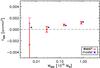 |
Fig. 4 Estimated SZ flux Y500 (in a sphere of radius r500) as a function of the mass M500 averaged in 4 mass bins. Red diamonds are the WMAP data. Blue stars correspond to the X-ray based model predictions and are shifted to higher masses by 20% for clarity. The model is in very good agreement with the data. |
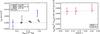 |
Fig. 5 Evolution of the Y500-M500
relation. Left: the WMAP data from Fig. 4 are divided into three redshift bins:
z < 0.08 (blue diamonds),
0.08 < z < 0.18
(green crosses), z > 0.18 (red triangles).
We observe the expected trend: at fixed mass, Y500
decreases with redshift. This redshift dependence is mainly due to the angular
distance
(Y500 ∝ Dang(z)-2).
The stars give the prediction of the model. Right: we divide
Y500 by |

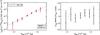 |
Fig. 6 Left: zoom on the >5 × 10¹³ M⊙ mass range of the Y500−M500 relation shown in Fig. 4. The data points and model stars are now scaled with the expected redshift dependence and are placed at the mean mass of the clusters in each bin. Right: ratio between data and model. |
7. The YSZ–M500 relation and its evolution
In this section, we study the mass and redshift dependence of the SZ signal and check it against the X-ray based model. Furthermore, we fit the Y500−M500 relation and compare it with the X-ray predictions.
7.1. Mass dependence and redshift evolution
Figure 4 shows the bin averaged SZ flux measurement as a function of mass compared to the X-ray based model prediction. As expected, the SZ cluster flux increases as a function of mass and is compatible with the model. In order to study the behaviour of the SZ flux with redshift, we subdivide each of the four mass bins into three redshift bins corresponding to the following ranges: z < 0.08, 0.08 < z < 0.18, z > 0.18. The result is shown in the left panel of Fig. 5. In a given mass bin the SZ flux decreases with redshift, tracing the Dang(z)-2 dependence of the flux. In particular, in the highest mass bin (1015 M⊙), the SZ flux decreases from 0.007 to 0.001 arcmin2 while the redshift varies from z < 0.08 to z > 0.18. The mass and the redshift dependence are in good agreement with the model (stars) described in Sect. 3.
Since the Dang(z)-2 dependence is
the dominant effect in the redshift evolution, we multiply
Y500 by
Dang(z)2 and divide it by the
self-similar mass dependence .
The expected self-similar behaviour of the new quantity
 as a
function of redshift is
E(z)2/3 (see Eq. (5)). The right panel of Fig. 5 shows as a
function of redshift for the three redshift bins
z < 0.08,
0.08 < z < 0.18,
z > 0.18. The points have been centered at the
average value of the cluster redshifts in each bin. The model is displayed as blue stars.
Since the model has a self-similar redshift dependence and
E(z)2/3 increases only
by a factor of 5% over the studied redshift range, the model stays nearly constant. The
blue dotted line is plotted through the model and varies as
E(z)2/3. The data points
are in good agreement with the model, but clearly, the redshift leverage of the sample is
insufficient to put strong constraints on the evolution of the scaling laws.
as a
function of redshift is
E(z)2/3 (see Eq. (5)). The right panel of Fig. 5 shows as a
function of redshift for the three redshift bins
z < 0.08,
0.08 < z < 0.18,
z > 0.18. The points have been centered at the
average value of the cluster redshifts in each bin. The model is displayed as blue stars.
Since the model has a self-similar redshift dependence and
E(z)2/3 increases only
by a factor of 5% over the studied redshift range, the model stays nearly constant. The
blue dotted line is plotted through the model and varies as
E(z)2/3. The data points
are in good agreement with the model, but clearly, the redshift leverage of the sample is
insufficient to put strong constraints on the evolution of the scaling laws.
We now focus on the mass dependence of the relation. We scale the SZ flux with the expected redshift dependence and plot it as a function of mass. The result is shown in Fig. 6 for the high mass end. The figure shows a very good agreement between the data points and the model, which is confirmed by fitting the relation to the individual SZ flux measurements (see next section).
7.2. Y500−M500 relation fit
Using the individual Y500 measurements and
M500 estimated from the X-ray luminosity, we fit a relation
of the form: 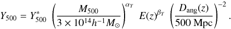 (13)The results are presented
in Table 3 for the analysis undertaken using the
REXCESS and that using the intrinsic
L500−M500 relation. The pivot
mass
3 × 10¹⁴h-1 M⊙,
close to that used by Arnaud et al. (2010), is
slightly larger than the average mass of the sample
(2.8|2.5 × 10¹⁴ M⊙ for the
REXCESS|intrinsic L500−M500
relation, respectively). We use a non-linear least-squares fit built on a
gradient-expansion algorithm (IDL curvefit function). In the fitting procedure, only the
statistical errors given by the matched multifilter
(σY500) are taken into
account. The total errors on the final fitted parameters, taking into account
uncertainties in X-ray properties, are estimated by Monte Carlo as described in
Sect. 5.
(13)The results are presented
in Table 3 for the analysis undertaken using the
REXCESS and that using the intrinsic
L500−M500 relation. The pivot
mass
3 × 10¹⁴h-1 M⊙,
close to that used by Arnaud et al. (2010), is
slightly larger than the average mass of the sample
(2.8|2.5 × 10¹⁴ M⊙ for the
REXCESS|intrinsic L500−M500
relation, respectively). We use a non-linear least-squares fit built on a
gradient-expansion algorithm (IDL curvefit function). In the fitting procedure, only the
statistical errors given by the matched multifilter
(σY500) are taken into
account. The total errors on the final fitted parameters, taking into account
uncertainties in X-ray properties, are estimated by Monte Carlo as described in
Sect. 5.
Fitted parameters for the observed YSZ–M500 relation.
 , in agreement
with the X-ray prediction
, in agreement
with the X-ray prediction  (at
0.4σ). Then, we relax the constraint on αY
and fit the normalisation and mass dependence at the same time. We obtain a value for
αY = 1.79, slightly greater than the self-similar
expectation (5/3) by 0.8σ. To study the redshift dependence of the
effect, we fix the mass dependence to
αY = 5/3 and fit
(at
0.4σ). Then, we relax the constraint on αY
and fit the normalisation and mass dependence at the same time. We obtain a value for
αY = 1.79, slightly greater than the self-similar
expectation (5/3) by 0.8σ. To study the redshift dependence of the
effect, we fix the mass dependence to
αY = 5/3 and fit
 and
βY at the same time. We obtain a somewhat stronger evolution
βY = 1.05 than the self-similar expectation (2/3). The
difference, however, is not significant (0.2σ). As already mentioned
above (see also Fig. 5 right), the redshift leverage
is too small to get interesting constraints on βY.
and
βY at the same time. We obtain a somewhat stronger evolution
βY = 1.05 than the self-similar expectation (2/3). The
difference, however, is not significant (0.2σ). As already mentioned
above (see also Fig. 5 right), the redshift leverage
is too small to get interesting constraints on βY.
As cluster mass estimates depend on the assumption of the underlying L500−M500 relation, so does the derived Y500−M500 relation as well. However, the effect is small. The normalisation is shifted from (1.60 ± 0.14 stat[±0.19 tot]) 10-3 arcmin2 to (1.37 ± 0.12 stat[±0.17 tot]) 10-3 arcmin2 when using the intrinsic L500−M500 relation. The difference is less than two statistical sigmas, and for the mass exponent, it is less than one.
8. Discussion and conclusions
In this paper we have investigated the SZ effect and its scaling with mass and X-ray luminosity using WMAP 5-year data of the largest published X-ray-selected cluster catalogue to date, derived from the combined NORAS and REFLEX samples. Cluster SZ flux estimates were made using an optimised multifrequency matched filter. Filter optimisation was achieved through priors on the pressure distribution (i.e., cluster shape) and the integration aperture (i.e., cluster size). The pressure distribution is assumed to follow the universal pressure profile of Arnaud et al. (2010), derived from X-ray observations of the representative local REXCESS sample. This profile is the most realistic available for the general population at this time, and has been shown to be in good agreement with recent high-quality SZ observations from SPT (Plagge et al. 2010). Furthermore, our analysis takes into account the dispersion in the pressure distribution. The integration aperture is estimated from the L500−M500 relation of the same REXCESS sample. We emphasise that these two priors determine only the input spatial distribution of the SZ flux for use by the multifrequency matched filters; the priors give no information on the amplitude of the measurement. As the analysis uses minimal X-ray data input, the measured and X-ray predicted SZ fluxes are essentially independent.
We studied the YSZ−LX relation using both bin averaged analyses and individual flux measurements. The fits using individual flux measurements give quantitative results for calibrating the scaling laws. The bin averaged analyses allow a direct quantitative check of SZ flux measurements versus X-ray model predictions based on the universal pressure profile derived by Arnaud et al. (2010) from REXCESS. An excellent agreement is found.
Using WMAP 3-year data, both Lieu et al. (2006) and Bielby & Shanks (2007) found that the SZ signal strength is lower than predicted given expectations from the X-ray properties of their clusters, concluding that that there is some missing hot gas in the intra-cluster medium. The excellent agreement between the SZ and X-ray properties of the clusters in our sample shows that there is in fact no deficit in SZ signal strength rel ative to expectations from X-ray observations. Due to the large size and homogeneous nature of our sample, and the internal consistency of our baseline cluster model, we believe our results to be robust in this respect. We note that there is some confusion in the literature regarding the phrase “missing baryons”. The “missing baryons” mentioned by Afshordi et al. (2007) in the WMAP 3-year data are missing with respect to the universal baryon fraction, but not with respect to the expectations from X-ray measurements. Afshordi et al. (2007) actually found good agreement between the strength of the SZ signal and the X-ray properties of their cluster sample, a conclusion that agrees with our results. This good convergence between SZ direct measurements and X-ray data is an encouraging step forward for the prediction and interpretation of SZ surveys.
Using L500 as a mass proxy, we also calibrated the Y500−M500 relation, finding a normalisation in excellent agreement with X-ray predictions based on the universal pressure profile, and a slope consistent with self-similar expectations. However, there is some indication that the slope may be steeper, as also indicated from the REXCESS analysis when using the best fitting empirical M500-YX relation (Arnaud et al. 2010). M500 depends on the assumed L500−M500 relation, making the derived Y500−M500 relation sensitive to Malmquist bias which we cannot fully account for in our analysis. However, we have shown that the effect of Malmquist bias on the present results is less than 2σ (statistical).
Regarding evolution, we have shown observationally that the SZ flux is indeed sensitive to
the angular size of the cluster through the diameter distance effect. For a given mass, a
low redshift cluster has a bigger integrated SZ flux than a similar system at high redshift,
and the redshift dependence of the integrated SZ flux is dominated by the angular diameter
distance ( ). However, the redshift
leverage of the present cluster sample is too small to put strong contraints on the
evolution of the Y500−L500 and
Y500−M500 relations. We have
nevertheless checked that the observed evolution is indeed compatible with the self-similar
prediction.
). However, the redshift
leverage of the present cluster sample is too small to put strong contraints on the
evolution of the Y500−L500 and
Y500−M500 relations. We have
nevertheless checked that the observed evolution is indeed compatible with the self-similar
prediction.
In this analysis, we have compensated for the poor sensitivity and resolution of the WMAP experiment (regarding SZ science) with the large number of known ROSAT clusters, leading to self-consistent and robust results. We expect further progress using upcoming Planck all-sky data. While Planck will offer the possibility of detecting the clusters used in this analysis to higher precision, thus significantly reducing the uncertainty on individual measurements, the question of evolution will not be answered with the present RASS sample due to its limited redshift range. A complementary approach will thus be to obtain new high sensitivity SZ observations of a smaller sample. The sample must be representative, cover a wide mass range, and extend to higher z (e.g., XMM-Newton follow-up of samples drawn from Planck and ground based SZ surveys). This would deliver efficient constraints not only on the normalisation and slope of the YSZ−LX and YSZ−M relations, but also their evolution, opening the way for the use of SZ surveys for precision cosmology.
Since we consider a standard self-similar model, we used the power law relations given in Appendix B of Arnaud et al. (2010). They are derived as in Pratt et al. (2009) with the same luminosity data but for masses derived from a standard slope M500−YX relation.
Acknowledgments
The authors wish to thank the anonymous referee for useful comments. J.-B. Melin thanks R. Battye for suggesting introduction of the h dependance into the presentation of the results. The authors also acknowledge the use of the HEALPix package (Górski et al. 2005) and of the Legacy Archive for Microwave Background Data Analysis (LAMBDA). Support for LAMBDA is provided by the NASA Office of Space Science. We also acknowledge use of the Planck Sky Model, developed by the Component Separation Working Group (WG2) of the Planck Collaboration, for the estimation of the radio source flux in the clusters and for the development of the matched multifilter, although the model was not directly used in the present work.
References
- Afshordi, N., Lin, Y.-T., Nagai, D., & Sanderson, A. J. R. 2007, MNRAS, 378, 293 [NASA ADS] [CrossRef] [Google Scholar]
- Arnaud, M., Pointecouteau, E., & Pratt, G. W. 2007, A&A, 474, L37 [NASA ADS] [CrossRef] [EDP Sciences] [Google Scholar]
- Arnaud, M., Pratt, G. W., Piffaretti, R., et al. 2010, A&A, 517, A92 [NASA ADS] [CrossRef] [EDP Sciences] [Google Scholar]
- Atrio-Barandela, F., Kashlinsky, A., Kocevski, D., & Ebeling, H. 2008, ApJ, 675, L57 [NASA ADS] [CrossRef] [Google Scholar]
- Bennett, C. L., Halpern, M., Hinshaw, G., et al. 2003, ApJS, 148, 1 [NASA ADS] [CrossRef] [Google Scholar]
- Bielby, R. M., & Shanks, T. 2007, MNRAS, 382, 1196 [NASA ADS] [CrossRef] [Google Scholar]
- Böhringer, H., Voges, W., Huchra, J. P., et al. 2000, ApJS, 129, 435 [NASA ADS] [CrossRef] [Google Scholar]
- Böhringer, H., Schuecker, P., Guzzo, L., et al. 2004, A&A, 425, 367 [NASA ADS] [CrossRef] [EDP Sciences] [Google Scholar]
- Böhringer, H., Schuecker, P., Pratt, G. W., et al. 2007, A&A, 469, 363 [NASA ADS] [CrossRef] [EDP Sciences] [Google Scholar]
- Bonamente, M., Joy, M., LaRoque, S. J., et al. 2008, ApJ, 675, 106 [NASA ADS] [CrossRef] [Google Scholar]
- Carlstrom, J. E., Ade, P. A. R., Aird, K. A., et al. 2009, PASP, submitted [arXiv:0907.4445] [Google Scholar]
- Condon, J. J., Cotton, W. D., Greisen, E. W., et al. 1998, AJ, 115, 1693 [NASA ADS] [CrossRef] [Google Scholar]
- Croston, J. H., Pratt, G. W., Böhringer, H., et al. 2008, A&A, 487, 431 [NASA ADS] [CrossRef] [EDP Sciences] [Google Scholar]
- da Silva, A. C., Kay, S. T., Liddle, A. R., & Thomas, P. A. 2004, MNRAS, 348, 1401 [NASA ADS] [CrossRef] [Google Scholar]
- Delabrouille, J., Cardoso, J.-F., Le Jeune, M., et al. 2009, A&A, 493, 835 [NASA ADS] [CrossRef] [EDP Sciences] [Google Scholar]
- Diego, J. M., & Partridge, B. 2009, MNRAS, 1927 [Google Scholar]
- Fosalba, P., Gaztañaga, E., & Castander, F. J. 2003, ApJ, 597, L89 [NASA ADS] [CrossRef] [Google Scholar]
- Górski, K. M., Hivon, E., Banday, A. J., et al. 2005, ApJ, 622, 759 [NASA ADS] [CrossRef] [Google Scholar]
- Hallman, E. J., O’Shea, B. W., Burns, J. O., et al. 2007, ApJ, 671, 27 [NASA ADS] [CrossRef] [Google Scholar]
- Halverson, N. W., Lanting, T., Ade, P. A. R., et al. 2009, ApJ, 701, 42 [NASA ADS] [CrossRef] [Google Scholar]
- Hernández-Monteagudo, C., Genova-Santos, R., & Atrio-Barandela, F. 2004, ApJ, 613, L89 [NASA ADS] [CrossRef] [Google Scholar]
- Hernández-Monteagudo, C., Macías-Pérez, J. F., Tristram, M., & Désert, F.-X. 2006, A&A, 449, 41 [NASA ADS] [CrossRef] [EDP Sciences] [Google Scholar]
- Herranz, D., Sanz, J. L., et al. 2002, MNRAS, 336, 1057 [NASA ADS] [CrossRef] [Google Scholar]
- Hinshaw, G., Nolta, M. R., Bennett, C. L., et al. 2007, ApJS, 170, 288 [NASA ADS] [CrossRef] [Google Scholar]
- Hinshaw, G., Weiland, J. L., Hill, R. S., et al. 2009, ApJS, 180, 225 [NASA ADS] [CrossRef] [Google Scholar]
- Kitayama, T., Komatsu, E., Ota, N., et al. 2004, PASJ, 56, 17 [NASA ADS] [Google Scholar]
- Kravtsov, A. V., Vikhlinin, A., & Nagai, D. 2006, ApJ, 650, 128 [NASA ADS] [CrossRef] [Google Scholar]
- Lieu, R., Mittaz, J. P. D., & Zhang, S.-N. 2006, ApJ, 648, 176 [NASA ADS] [CrossRef] [Google Scholar]
- Lamarre, J. M., Puget, J. L., Bouchet, F., et al. 2003, New Astron. Rev., 47, 1017 [Google Scholar]
- Marrone, D. P., Smith, G. P., Richard, J., et al. 2009, ApJ, 701, L114 [NASA ADS] [CrossRef] [Google Scholar]
- Mauch, T., Murphy, T., Buttery, H. J., et al. 2003, MNRAS, 342, 1117 [NASA ADS] [CrossRef] [Google Scholar]
- Melin, J.-B., Bartlett, J. G., & Delabrouille, J. 2006, A&A, 459, 341 [NASA ADS] [CrossRef] [EDP Sciences] [Google Scholar]
- Motl, P. M., Hallman, E. J., Burns, J. O., & Normal, M. L. 2005, ApJ, 623, L63 [NASA ADS] [CrossRef] [Google Scholar]
- Mroczkowski, T., Bonamente, M., Carlstrom, J., et al. 2009, ApJ, 694, 1034 [NASA ADS] [CrossRef] [Google Scholar]
- Myers, A. D., Shanks, T., Outram, P. J., Frith, W. J., & Wolfendale, A. W. 2004, MNRAS, 347, L67 [NASA ADS] [CrossRef] [Google Scholar]
- Nagai, D., Kravtsov, A. V., & Vikhlinin, A. 2007, ApJ, 668, 1 [NASA ADS] [CrossRef] [Google Scholar]
- Nord, M., Basu, K., Pacaud, F., et al. 2009, A&A, 506, 623 [NASA ADS] [CrossRef] [EDP Sciences] [Google Scholar]
- Plagge, T., Benson, B., Ade, P. A. R., et al. 2010, ApJ, 716, 1118 [NASA ADS] [CrossRef] [Google Scholar]
- Pratt, G. W., Croston, J. H., Arnaud, M., Böhringer, H. 2009, A&A, 498, 361 [NASA ADS] [CrossRef] [EDP Sciences] [Google Scholar]
- Staniszewski, Z., Ade, P. A. R., Aird, K. A., et al. 2009, ApJ, 701, 32 [CrossRef] [Google Scholar]
- Sunyaev, R. A., & Zel’dovich, Ya. B. 1970, Comments Astrophys. Space Phys., ComAp, 2, 66 [NASA ADS] [Google Scholar]
- Sunyaev, R. A., & Zel’dovich, Ya. B. 1972, Comments Astrophys. Space Phys., 4, 173 [NASA ADS] [EDP Sciences] [Google Scholar]
- Valenziano, L., et al. 2007, New Astron. Rev., 51, 287 [NASA ADS] [CrossRef] [Google Scholar]
- Vikhlinin, A., Burenin, R., Ebeling, H., et al. 2009, ApJ, 692, 1033 [NASA ADS] [CrossRef] [Google Scholar]
Appendix A: SZ flux definitions
In this Appendix, we give the definitions of SZ fluxes we used. Table A.1 gives the equivalence between them. In this paper,
we mainly use Y500 as the definition of the SZ flux. This flux
is the integrated SZ flux from a sphere of radius r500. It can
be related to Ynr500, the flux from a sphere
of radius n × r500 by integrating over the
cluster profile: 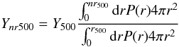 (A.1)where
P(r) is given by Eq. (3). The ratio
Ynr500/Y500
is given in Table A.1 for
n = 1, 2 ,3 ,5 ,10.
(A.1)where
P(r) is given by Eq. (3). The ratio
Ynr500/Y500
is given in Table A.1 for
n = 1, 2 ,3 ,5 ,10.
In practice, an experiment does not directly measure Y500 but
the SZ signal of a cluster integrated along the line of sight and within an angular
aperture. This corresponds to the Compton parameter integrated over a cylindrical volume.
In Sect. 4, we estimate
, the flux
from a cylinder of aperture radius 5 × r500 using the matched
multifilter. Given the cluster profile, we can derive
Ynr500 from
 :
:
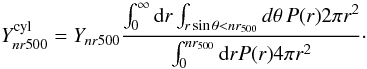 (A.2)The ratio
 is given in
Table A.1 for
n = 1, 2 ,3 ,5 ,10.
In the paper, we calculate Y500 from
is given in
Table A.1 for
n = 1, 2 ,3 ,5 ,10.
In the paper, we calculate Y500 from
 .
.
Equivalence of SZ flux definitions
Appendix B: SZ units conversion
In this Appendix, we provide the numerical factor needed for the SZ flux units conversion and derive the relation between the recently introduced YX parameter and the SZ flux YSZ. The latter will allow readers to easily convert between SZ fluxes given in this paper and those reported in other publications.
Given the definition of SZ flux:
 (B.1)where
Ωnr500 is the solid angle covered by
n × r500, and the fact that the Compton
parameter y is unitless, the observational units for the SZ flux are
those of a solid angle and usually given in arcmin2.
(B.1)where
Ωnr500 is the solid angle covered by
n × r500, and the fact that the Compton
parameter y is unitless, the observational units for the SZ flux are
those of a solid angle and usually given in arcmin2.
The SZ flux can be also computed in units of Mpc2 and the conversion is given
by ![\appendix \setcounter{section}{2} \begin{eqnarray} Y_{\rm SZ} [{\rm Mpc}^2] & = & 60^{-2} \, \left ( {\pi \over 180} \right )^2 \, Y_{\rm SZ} [{\rm arcmin}^2] \, \left ( D_{\rm ang}(z) \over 1 \, {\rm Mpc} \right )^2 \nonumber\\ & = & 8.46 \times 10^{-8} \, Y_{\rm SZ} [{\rm arcmin}^2] \, \left ( D_{\rm ang}(z) \over 1~{\rm Mpc} \right )^2 \end{eqnarray}](/articles/aa/full_html/2011/01/aa13999-10/aa13999-10-eq236.png) (B.2)where
Dang(z) is the angular distance to the
cluster.
(B.2)where
Dang(z) is the angular distance to the
cluster.
The X-ray analogue of the integrated SZ Comptonisation parameter is
YX = Mgas,500TX
whose natural units are M⊙ keV, where
Mgas,500 is the gas mass in
r500 and TX is the
spectroscopic temperature excluding the central
0.15 r500 region (Kravtsov
et al. 2006). To convert between YSZ and
YX, we first have
![\appendix \setcounter{section}{2} \begin{equation} Y_{\rm SZ} [{\rm Mpc}^2] = {\int_0^{r_{500}} {\rm d}r \, \sigma_{\rm T} \, {T_{\rm e}(r) \over m_{\rm e} c^2} \, n_{\rm e}(r) 4 \pi r^2} \end{equation}](/articles/aa/full_html/2011/01/aa13999-10/aa13999-10-eq242.png) (B.3)where
σT is the Thomson cross section (in Mpc2),
mec2 the electron mass (in keV),
Te(r) the electronic temperature (in keV)
and ne(r) the electronic density. By assuming
that the gas temperature Tg(r) is equal to
the electronic temperature Te(r) and writing
the gas density as
ρg(r) = μempne(r),
where mp is the proton mass and
μe = 1.14 the mean molecular weight per free electron, one
obtains:
(B.3)where
σT is the Thomson cross section (in Mpc2),
mec2 the electron mass (in keV),
Te(r) the electronic temperature (in keV)
and ne(r) the electronic density. By assuming
that the gas temperature Tg(r) is equal to
the electronic temperature Te(r) and writing
the gas density as
ρg(r) = μempne(r),
where mp is the proton mass and
μe = 1.14 the mean molecular weight per free electron, one
obtains: ![\appendix \setcounter{section}{2} \begin{eqnarray} Y_{\rm SZ} [{\rm Mpc}^2] & = & {\sigma_T \over m_{\rm e} c^2} {1 \over \mu_{\rm e} m_p} {\int_0^{r_{500}} {\rm d}r \, \rho_{\rm g}(r) \, T_{\rm g}(r) 4 \pi r^2} \nonumber\\ & = & C_{{\rm XSZ}} \, M_{{\rm gas},500} \, T_{\rm MW} = A \, C_{{\rm XSZ}} \, Y_{\rm X} \end{eqnarray}](/articles/aa/full_html/2011/01/aa13999-10/aa13999-10-eq251.png) (B.4)where,
as in Arnaud et al. (2010), we defined
(B.4)where,
as in Arnaud et al. (2010), we defined
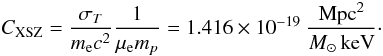 (B.5)The mass weighted
temperature is defined as:
(B.5)The mass weighted
temperature is defined as:
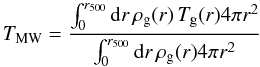 (B.6)and
the factor
A = TMW/TX
takes into account for the difference between mass weighted and spectroscopic average
temperatures. Arnaud et al. (2010) find
A ~ 0.924.
(B.6)and
the factor
A = TMW/TX
takes into account for the difference between mass weighted and spectroscopic average
temperatures. Arnaud et al. (2010) find
A ~ 0.924.
All Tables
Values for the parameters of the LX − M relation derived from REXCESS data (Pratt et al. 2009; Arnaud et al. 2010).
All Figures
|
Fig. 1 Inferred masses for the 893 NORAS/REFLEX clusters as a function of redshift. The cluster sample is flux limited. The right vertical axis gives the corresponding X-ray luminosities scaled by E(z)−7/3. The dashed blue lines delineate the mass range over which the L500−M500 relation from Pratt et al. (2009) was derived. |
| In the text | |
|
Fig. 2 Left: estimated SZ flux from a cylinder of aperture radius
5 × r500 ( |
| In the text | |
|
Fig. 3 Left: bin averaged SZ flux from a sphere of radius r500 (Y500) as a function of X-ray luminosity in a aperture of r500 (L500). The WMAP data (red diamonds and crosses), the SZ cluster signal expected from the X-ray based model (blue stars) and the combination of the Y500−M500 and L500−M500 relations (dash and dotted dashed lines) are given for two analyses, using respectively the intrinsic L500−M500 and the REXCESS L500−M500 relations. As expected, the data points do not change significantly from one case to the other showing that the Y500-L500 relation is rather insensitive to the finer details of the underlying L500−M500 relation. Right: ratio of data points to model for the two analysis. The points for the analysis undertaken with the intrinsic L500−M500 are shifted to lower luminosities by 20% for clarity. |
| In the text | |
|
Fig. 4 Estimated SZ flux Y500 (in a sphere of radius r500) as a function of the mass M500 averaged in 4 mass bins. Red diamonds are the WMAP data. Blue stars correspond to the X-ray based model predictions and are shifted to higher masses by 20% for clarity. The model is in very good agreement with the data. |
| In the text | |
|
Fig. 5 Evolution of the Y500-M500
relation. Left: the WMAP data from Fig. 4 are divided into three redshift bins:
z < 0.08 (blue diamonds),
0.08 < z < 0.18
(green crosses), z > 0.18 (red triangles).
We observe the expected trend: at fixed mass, Y500
decreases with redshift. This redshift dependence is mainly due to the angular
distance
(Y500 ∝ Dang(z)-2).
The stars give the prediction of the model. Right: we divide
Y500 by |
| In the text | |
|
Fig. 6 Left: zoom on the >5 × 10¹³ M⊙ mass range of the Y500−M500 relation shown in Fig. 4. The data points and model stars are now scaled with the expected redshift dependence and are placed at the mean mass of the clusters in each bin. Right: ratio between data and model. |
| In the text | |
Current usage metrics show cumulative count of Article Views (full-text article views including HTML views, PDF and ePub downloads, according to the available data) and Abstracts Views on Vision4Press platform.
Data correspond to usage on the plateform after 2015. The current usage metrics is available 48-96 hours after online publication and is updated daily on week days.
Initial download of the metrics may take a while.