| Issue |
A&A
Volume 694, February 2025
ZTF SN Ia DR2
|
|
|---|---|---|
| Article Number | A5 | |
| Number of page(s) | 8 | |
| Section | Cosmology (including clusters of galaxies) | |
| DOI | https://doi.org/10.1051/0004-6361/202450391 | |
| Published online | 14 February 2025 | |
ZTF SN Ia DR2: Evidence of changing dust distribution with redshift using type Ia supernovae
1
Université Claude Bernard Lyon 1, CNRS, IP2I Lyon/IN2P3, IMR 5822, F-69622 Villeurbanne, France
2
Department of Physics, Lancaster University, Lancs LA1 4YB, UK
3
Sorbonne Université, CNRS/IN2P3, LPNHE, F-75005 Paris, France
4
The Oskar Klein Centre, Department of Physics, AlbaNova, SE-106 91 Stockholm, Sweden
5
School of Physics, Trinity College Dublin, College Green, Dublin 2, Ireland
6
National Research Council of Canada, Herzberg Astronomy & Astrophysics Research Centre, 5071 West Saanich Road, Victoria BC V9E 2E7, Canada
7
Université Clermont Auvergne, CNRS/IN2P3, LPCA, F-63000 Clermont-Ferrand, France
8
Aix Marseille Université, CNRS/IN2P3, CPPM, Marseille, France
9
Department of Physics, Duke University Durham, NC 27708, USA
10
Institute of Astronomy and Kavli Institute for Cosmology, University of Cambridge, Madingley Road, Cambridge CB3 0HA, UK
11
Institute of Space Sciences (ICE-CSIC), Campus UAB, Carrer de Can Magrans, s/n, E-08193 Barcelona, Spain
12
Institut d’Estudis Espacials de Catalunya (IEEC), 08860 Castelldefels (Barcelona), Spain
13
Division of Physics, Mathematics & Astronomy, California Institute of Technology, Pasadena, CA 91125, USA
14
The Oskar Klein Centre, Department of Astronomy, Stockholm University, AlbaNova, SE-106 91 Stockholm, Sweden
15
Nordic Optical Telescope, Rambla José Ana Fernández Pérez 7, ES-38711 Breña Baja, Spain
16
Lawrence Berkeley National Laboratory, 1 Cyclotron Road, MS 50B-4206, Berkeley CA 94720, USA
17
Department of Astronomy, University of California, Berkeley, 501 Campbell Hall, Berkeley CA 94720, USA
⋆ Corresponding author; b.popovic@ip2i.in2p3.fr
Received:
15
April
2024
Accepted:
1
August
2024
Context. Type Ia supernova (SNIa) are excellent probes of local distance and the growing sample sizes of SNIa have driven an increased propensity to study the associated systematic uncertainties and improve standardisation methods in preparation for the next generation of cosmological surveys into the dark energy equation of state, w.
Aims. We aim to probe the potential change in the SNIa standardisation parameter, c, with redshift and the host-galaxy of the supernova. Improving the standardisation of SNIa brightness measurements will require the relationship between the host and the SNIa to be accounted for. In addition, potential shifts in the SNIa standardisation parameters with redshift will cause biases in the recovered cosmology.
Methods. In this work, we assembled a volume-limited sample of 3000 likely SNIa across a redshift range from z = 0.015 to z = 0.36. This sample was fitted with changing mass and redshift bins to determine the relationship between the intrinsic properties of SNe Ia and their redshift and host galaxy parameters. We then investigated the colour-luminosity parameter, β, as a subsequent test of the SNIa standardisation process.
Results. We find that the changing colour distribution of SNe Ia with redshift is driven by dust at a confidence of > 4σ. Additionally, we show a strong correlation between the host galaxy mass and the colour-luminosity coefficient β (> 4σ), even when accounting for the quantity of dust in a host galaxy.
Conclusions. These results indicate that the observed colour distribution of SNe Ia does change with redshift. However, we note that this is an observational effect, rather than an intrinsic change. Future cosmological measurements with SNe Ia must take into account these changing dust distributions to reduce the number of potential sources of systematic uncertainty.
Key words: supernovae: general / cosmology: observations / dark energy
© The Authors 2025
 Open Access article, published by EDP Sciences, under the terms of the Creative Commons Attribution License (https://creativecommons.org/licenses/by/4.0), which permits unrestricted use, distribution, and reproduction in any medium, provided the original work is properly cited.
This article is published in open access under the Subscribe to Open model. Subscribe to A&A to support open access publication.
1. Introduction
The discovery of the accelerating expansion of the universe (Riess et al. 1998; Perlmutter et al. 1999) was undertaken using standardised type Ia supernovae (SNe Ia). The cause of this accelerating expansion remains an unsolved mystery, but the standard model of cosmology associates it to a cosmological constant Λ; or, more generically, to dark energy. The two decades between the discovery of the accelerating expansion and have now seen sample sizes of SNe Ia grow from tens of supernovae to thousands. Modern measurements of the dark energy equation-of-state parameter, w, have statistical uncertainties on the order of ∼0.02 (Brout et al. 2022; Vincenzi et al. 2024; Popovic et al. 2024) and this field of research will soon be dominated by the relative systematic uncertainties. The decreasing statistical uncertainties place a greater emphasis on understanding the systematic uncertainties that are inherent with respect to measurements of cosmology undertaken using SNe Ia.
Here, we further improve on previous works that study the correlation between the properties of SNe Ia and their host galaxies (Sullivan et al. 2010; Rigault et al. 2013; Uddin et al. 2017; Rigault et al. 2020; Popovic et al. 2021). Most cosmology analyses with SNe Ia use a variation of the SALT (Guy et al. 2010) framework to fit type Ia supernova (SNIa) light curves and standardise their brightness. SALT uses two parameters to standardise the SNIa brightness: a stretch parameter, x1, which encompasses the luminosity dependence on light curve duration and a colour parameter, c, which describes the wavelength-dependent luminosity. Since the study of Kelly et al. (2010), Sullivan et al. (2010), these two parameters have been joined by an ad hoc correction, the ‘mass step’, that accounts for the otherwise unexplained observed correlation between the standardised brightness of the SNIa and the properties of their host galaxy.
Correlations between SNIa properties and their environment have long been studied in the context of SN cosmology. Early on, the correlation between the light curve stretch and the host parameters was demonstrated (e.g. Hamuy et al. 1996; Howell et al. 2007; Sullivan et al. 2010; Lampeitl et al. 2010). Recently, with increased statistical power, progress has been made into uncovering underlying reasons for the correlations between fitted SALT properties (e.g., x1, c) and the properties of the host galaxies of the SNe Ia. While Popovic et al. (2021) found strong evidence that both x1 and c change with the host galaxy mass, Nicolas et al. (2021) provided an analytical description of changing x1 values with both host galaxy mass and the local specific star formation rate (LsSFR). However, this refined description was insufficient to explain the mass step. In the last decades, several explanations arose to find the origin of the mass-step, with the aim to correctly account for this SN astrophysical dependency while fitting cosmological parameters. Rigault et al. (2013, 2020) and Briday et al. (2022), following earlier works on SN rates (e.g. Sullivan et al. 2006) suggest that prompt and delayed SNe Ia have intrinsically different absolute magnitudes. In that model, the prompt SNe, associated with recent star formation, are fainter, and the mass-step originates from the fact that massive galaxies host few prompt SNe Ia (see also: e.g. Childress et al. 2013, 2014).
Recently, following on prior works (from e.g. Mandel et al. 2017) Brout & Scolnic (2021) provided an explanation that is disconnected from the prompt and delayed-rate model. They show that the amplitude of the mass-step depends on the SN colour and were able explain the variation (and, consequently, the mass-step) by allowing the colour-magnitude relation to change as a function of host-mass. This model, further developed in Popovic et al. (2023), Kelsey et al. (2023), and Wiseman et al. (2022), follows the assumption that the redder end of the SN Ia color distribution is caused by dust, whose properties varies as a function of host stellar mass. This dust model describes the data well (Popovic et al. 2023).
While both approaches (dust or age) have their benefits and their limitations with respect to unveiling the true origin of the observed astrophysical biases is of paramount importance for SN cosmology as the resulting modelling for deriving distances may impact the measurement of cosmological parameters. In this analysis, we use the second data release of the Zwicky Transient Facility (ZTF; Bellm et al. 2019; Graham et al. 2019; Masci et al. 2019) SNIa sample (ZTF Data Release Paper), with spectra from Blagorodnova et al. (2018), Rigault et al. (2019). This release (ZTF-Cosmo-DR2) contains ∼3000 cosmological-quality SNe Ia at z < 0.1. Combined with recent improvements in the reliability of non-spectroscopically confirmed SNIa samples (Vincenzi et al. 2024; Popovic et al. 2024), we present the largest study of the evolution of the SNIa colour and colour-magnitude relation with redshift.
This study is important for the future of studies of the equation of state, w. Combining constraints from SNe Ia with external probes provides exquisite measurements of the properties of our universe, as in Vincenzi et al. (2024) and DESI Collaboration (2024). Systematics that evolve with redshift are degenerate with different cosmologies. With recent results from DESI Collaboration (2024) that indicate a non-static w may be preferred, even-further increased control of systematic uncertainties will be needed for the next generation of measurements of cosmology with SNe Ia.
The overview of the paper is as follows: Section 2 provides an overview of the data: ZTF, SDSS, PS1, and DES, alongside quality cuts and light curve fitting parameters. Section 3 explains the methodology used to define and fit the sample to explore evolution of c with redshift and mass. Section 4 presents the results and any potential evolution of c with other SNIa parameters, while Sects. 5 and 6, respectively, present the discussion and conclusions.
2. Data
High- and low-redshift surveys require different cadences, sky-coverage, and overall survey strategies. In order to maximise the statistics and redshift range, samples of SNIa are often combined, as in Amanullah et al. (2010), Betoule et al. (2014), Brout et al. (2022), Popovic et al. (2024).
We make use of the SNIa samples from the Zwicky Transient Facility (ZTF; ZTF Data Release Paper), the Sloan Digital Sky Survey (SDSS; Frieman et al. 2008; Sako et al. 2018; Popovic et al. 2020), Pan-STARRS (PS1; Jones et al. 2018), and Dark Energy Survey 5-year (DES; Vincenzi et al. 2024). Table 1 provides a summary of the dataset used in this analysis, showing the magnitude limit of the telescope, the resulting redshift cut, and the number of SNe in the final sample. We include an additional conservative sample, with a stricter redshift cut, that is shown in parentheses. This is explained further in Sect. 3.
Summary of redshift cuts for fiducial (Fid) and conservative (Con) samples after other quality cuts.
The second ZTF data release covers the years of 2018 to 2020. The survey overview is presented in ZTF Data Release Paper. Light curve data typical have a two-day cadence in g and r and a 5 day cadence in i. All SNe Ia have a spectroscopic classification and about half have a host-galaxy redshift with the typical precision of 10−4. For the other half, the data release relies on SN spectroscopic feature that has been shown to have an unbiased redshift precision of 10−3. Table 2 shows a summary of the ZTF sample compared to the largest historic low-redshift surveys of SNe Ia; while all cover a similar redshift range (z < 0.1), ZTF is the first all-sky survey with statistics an order of magnitude larger than previous samples.
Comparison of ZTF with historical low-redshift samples.
The SDSS supernova programme was run for three observing seasons between 2005 to 2007. The survey overview is provided in Frieman et al. (2008). SDSS light curves have data in the ugriz bands with an average observing cadence of four days. We took light curves from Sako et al. (2018) and host galaxies and redshifts from Popovic et al. (2020). PS1 ran from 2009 to 2013, observing with the griz filters at a cadence of six observations every five days. The PS1 light curves were taken from Chambers et al. (2016), with host galaxy redshifts drawn from papers listed in Jones et al. (2018).
The DES-SN programme was run for five years, covering 23 deg2 across the sky. With an average observing cadence of even days, DES took data in the griz bands across eight ’shallow’ fields and two ‘deep’ fields, covering a balance between increased maximum redshift in the deep fields, which utilise multiple exposures and an area coverage and volume in the shallow fields; the data come from Sánchez et al. (2024).
SNe Ia at peak brightness are not uniform enough to support accurate measurements of cosmological parameters on their own; they require standardisation via a light curve modelling and fitting programme. We use the SALT2 programme introduced by Guy et al. (2010) with updated training from Taylor et al. (2021). The SALT fit returns four parameters for each SNIa: t0 the time of peak brightness; x0 the overall light curve amplitude; c the colour parameter; and x1, the stretch parameter related to the width of the light curve. These latter three parameters are directly used to standardise SNIa luminosity, μ, according to the Tripp estimator (Tripp 1998):

where mB = −2.5log10(x0), c and x1 are defined above, and M0 is the absolute magnitude of a SNIa, with c = x1 = 0. Then, α and β are the stretch-luminosity and colour-luminosity coefficients, respectively, and are defined for a given sample of SNIa.
For the data, we apply the following conventional cuts, following papers, such as Betoule et al. (2014), Scolnic et al. (2018), Brout et al. (2022):
-
σx1 < 1: SALT2 x1 uncertainty < 1,
-
σc < 0.1: SALT2 c uncertainty < 0.1,
-
σt0 < 1: Uncertainty on fitted peak brightness epoch < 1 days,
-
−4 < x1 < 4,
-
−0.3 < c < 0.8,
-
Trest,min < 5: requires at least 1 observation five days prior to peak brightness (rest frame),
-
Trest,max > 0: Requires at least 1 observation after peak brightness (rest frame).
With respect to the case for SDSS, PS1, and DES, we institute an additional cut, that the probability of a SN being a SNIa is greater than 0.9: PIa > 0.9. We make use of the SuperNNova classifier from Möller & de Boissière (2020), taking trained surfaces from Popovic et al. (2024) and Vincenzi et al. (2024). This cut is not applied for ZTF, which has a spectroscopic identification for the entire sample. The extra cut placed on the high redshift surveys ensures that the sample is comprised of SNe Ia and that the limiting magnitude of these surveys is determined by the survey photometry rather than the spectroscopic followup, bringing them in line with the ZTF sample.
3. Methodology
This work has been made possible thanks to the unprecedented redshift range and statistics of the ZTF sample. Combining ZTF with the higher-redshift surveys, SDSS, PS1, and DES, offers a volume-limited sample of ∼3500 SNe Ia, ranging from 0.04 < z < 0.36. This selection is larger than any previously assembled collection of SNe Ia.
Here, we outline the methodology used to assess the evolution of SNIa colour with redshift and host galaxy mass. In this section, we begin with the definition and creation of a volume-limited sample for each survey so as to remove potential biases arising from selection effects, then we split the samples into redshift and mass bins to fit the colour population within each bin.
One consequence of the need for standardisation for SNIa is that redder SNIa (those approaching c = 0.3) are dimmer than bluer supernovae. This presents a problem for investigating the colour evolution with redshift; as the redshift increases, surveys approach the magnitude limit of being able to observe objects. This Malmquist bias can impact inferred cosmologies and, indeed, our colour distributions as well.
There are two solutions to this magnitude limit. The first is the introduction of bias corrections from Kessler & Scolnic (2017), using realistic simulations to correct for limitations in observing the apparent magnitudes of SNIa. The second method is to create a ‘volume-limited’ sample. Since the purpose of this work is to find the underlying distribution of colour, we are not able to provide accurate bias corrections. Instead, we follow Nicolas et al. (2021) and define two volume limited samples for each survey: a fiducial survey and a conservative one.
To define the volume limited sample, we follow Nicolas et al. (2021). We use Equation 1 and assume that the absolute magnitude for an SNIa with c = x1 = 0 is M0 − 19.36. From this, we can calculate a brightness at time of maximum light M = M0 − αx1 + βc. Assuming a common β = 3.1 and α = 0.15 (Betoule et al. 2014; Scolnic et al. 2018; Brout et al. 2022), the faintest magnitude we would expect to see is approximately −18.31 mags, from a SNIa with x1 = −1.65 and c = 0.25. However, we require at least one observation before the peak brightness, which requires an even fainter magnitude, namely, at −18 for our fiducial limiting magnitude. Our conservative limiting magnitude is fainter, set at −17.5. In both cases, the limiting magnitudes we place are in reference to the SALT-fitted brightness.
With the limiting magnitudes and the magnitude limit of the surveys (taken from Nicolas et al. 2021, ZTF Data Release Paper), we were able to calculate a redshift, zlim, such that we expect the sample to be complete and free of magnitude-based selection effects below zlim. A review of the magnitude limits, limiting redshifts, and resulting number of SNIa is shown for each survey in Table 1. The redshift distributions for the full, fiducial, and conservative are shown in Fig. 1 for each survey included in this paper. We placed our redshift cuts on the sample after calculating the limiting redshift, zlim, from the SALT-fitted magnitude of the supernovae.
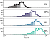 |
Fig. 1. Redshift distributions for ZTF, SDSS, PS1, and DES. The full sample is presented for each survey before any redshift cuts in unfilled histogram. The light fill represents the redshift range of the fiducial sample and the dark fill shows the redshift range of the conservative sample. For details, see Sect. 2. |
To investigate evolution of SNIa colour c with redshift, we quantile-bin our sample to create seven evenly populated bins of redshift. For the colour evolution with host galaxy stellar masses measured relative to the mass of our Sun (i.e. Sol = 1 M⊙, MStar = 10X M⊙; whereas here we report X), we made use of evenly spaced mass bins, so as to maintain a bin edge at MStar = 10 and to be consistent with literature involving the mass step at 10MStar.
In both cases, we fit within the individual bins of mass or redshift separately to find the apparent colour distribution. The change of the fit results in each bin can be assessed to determine any kind of evolution.
Within the individual bins, we made use of the fitting code from Ginolin et al. (2025) to fit the apparent colour via a convolution of a Gaussian intrinsic SNIa colour, cint, and an exponential dust component, Edust:

with a noise term: ϵnoise. The Gaussian and exponential tail is drawn as:
The minimisation process is done via MINUIT (James & Roos 1975), which also returns fitting errors that are used within the analysis. The errors recorded by MINUIT are symmetric Gaussians. We report these results with  as the mean of the Gaussian intrinsic colour distribution, cσ as the standard deviation, and EDust as the τ value describing the exponential distribution.
The choice here of an intrinsic Gaussian distribution that is reddened by external dust is taken from Brout & Scolnic (2021), but has recently gained traction with SNIa cosmology, used in such works as Wiseman et al. (2022), Kelsey et al. (2023), Popovic et al. (2021). It was also applied as the default model in the cosmology analyses performed by Brout et al. (2022), Vincenzi et al. (2024), Popovic et al. (2024).
Brout & Scolnic (2021) and Popovic et al. (2023) showed that while the observed SNIa colour distribution is an acceptable probe of the columnar density of dust EDust (e.g. the quantity of dust through the line-of-sight), it is not able to provide strong constraints on the Rv parameter. The best indicator of the Rv of the host galaxy, from SNIa data alone, is the colour-luminosity coefficient β. To further investigate the relationship between colour and host-galaxy properties, we investigate the relationship between host galaxy mass and the β parameter.
To fit β, we modify Equation (1):
where mB and x1 are as normally defined, and we float α alongside our β. μtheory is the theoretical distance modulus from a Flat ΛCDM cosmology with H0 = 74. The slope of this μ* value, when plotted against the supernova colour c, is β. We fit this slope, simultaneously with the intercept, using MINUIT in bins of mass to determine potential β evolution.
The masses reported in this paper have been taken from their respective data releases, namely: ZTF DR2 Data Release and Vincenzi et al. (2024) for ZTF and DES, or in the case of SDSS and PS1, the updated masses from Popovic et al. (2024). All surveys use consistent PEGASE.2 code with a Kroupa (2001) initial mass function. We used the same methodology and star formation history as in Smith et al. (2020); in short, the SED of each star formation history was initialised with a metallicity of 0.004, which evolves consistently, calculated at 102 time steps from 0 to 14 Gyr. We used seven foreground dust screens, with the colour excess ranging from 0 to 0.3 magnitudes.
4. Results
We present the results of the fitting process from Sect. 3 on the samples defined in Sect. 2. In Fig. 2 shows mB vs. redshift for the fiducial sample, alongside the demarcations for the quantile redshift bins. In the inset, we show the colour distributions of each of the redshift bins; here we investigate the cause of the apparent change in colour distribution. Significance measurements are calculated by comparing the binned results to the mean of the overall distribution and converting them to a significance measurement using the number of degrees of freedom.
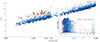 |
Fig. 2. mB vs. redshift for the SNIa in the Fiducial Sample defined in Table 1. Each supernova is colour coded according to its colour c. The grey vertical lines demark the quantile redshift bins, and the colour histogram is provided for each redshift bin in the inset plot. See Sect. 2 for more details. |
4.1. Evolution with redshift
We fit the colour distribution of the SNIa in each of the seven quantile redshift bins and present the inferred Gaussian+exponential distribution in Fig. 3.
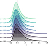 |
Fig. 3. Fit results for the quantile redshift bins of the fiducial sample. The c distribution is shown for each redshift bin and colour coded to become darker with increasing redshift. For details, see Sect. 4.1. |
We plotted the Gaussian and exponential parameters from Fig. 3 to more accurately assess any potential trends. We find that the Gaussian parameters that describe the SNIa colour distribution are consistent with no evolution.  changes with redshift at a confidence of < 1σ, and cσ changes with redshift at a confidence of 3.4σ. These low signals are in contrast with the EDust parameter, for which we find evidence of evolution with redshift at a confidence of > 6σ. For comparison, we show the χ2 values from the conservative sample that was detailed in Sect. 3. The conservative sample trends are qualitatively similar to the full sample, though the larger uncertainties that arise from the smaller sample decrease the evidence of EDust evolving from 6σ to 3σ (Fig. 4).
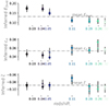 |
Fig. 4. Fit parameters for the Gaussian and exponential distributions plotted with increasing redshift. Alongside each parameter, the mean fit value is plotted in dash-dotted line to provide context. The fit results from the conservative sample are overlaid in triangles for comparison. See more in Sect. 4.1. |
Table 3 shows the χ2 breakdown for each of the parameters and their evolution with redshift. We see the trends from the fiducial sample (i.e. data that appear to prefer an evolving dust-based EDust parameter over a change in the intrinsic SNIa colour distribution) hold for the conservative sample, although we do find a confidence of > 5σ for EDust evolution in the conservative sample, instead of > 6σ.
Goodness-of-fit χ2 values for each parameter compared to the null hypothesis of no z-evolution, with seven DOF.
4.2. Evolution with mass
Figure 5 shows the evolution of the host galaxy mass with redshift. There is an under-density of SNe between z = 0.06 and z = 0.1; this under-density arises from the redshift cut on ZTF at z = 0.06, leaving only SDSS SNe in the range of 0.06 < z0.1. Even with this under-density we find no evidence of the median host galaxy mass changing with redshift (< 1σ from the median of the full distribution).
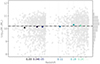 |
Fig. 5. Host galaxy mass plotted vs redshift for the Fiducial sample. Supernovae are shown in grey, the coloured circles represent the median host galaxy mass in each quantile redshift bin. The dash-dotted black line shows the median host galaxy mass of the entire sample. The mass distribution, marginalised over redshift, is shown on the right. See Sect. 4.2 for more details. |
Bolstered by the confidence that there is no correlation between the host galaxy mass and redshift, we show the evolution of the SNIa colour distribution with host galaxy mass. Figure 6 shows the change of colour distribution with host galaxy mass, binned in steps of 0.5MStar, starting at 8MStar and going to 11.5MStar. As a reminder, in contrast to the quantile binning for redshift, we do not require equal statistics in each bin, so that we can place a bin edge at the historical mass step value of 10MStar.
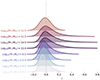 |
Fig. 6. Fit results for the host galaxy mass bins of the fiducial sample. The c distribution is shown for each mass bin, colour coded with increasing host galaxy mass. (Sect. 4.2). |
Figure 7 displays the individual parameters  , cσ, and EDust from the fitted results presented in Fig. 6. We show the χ2 values in Table 4 and we see results similar to the redshift distribution results. There is little evidence of the SNIa colour parameters changing, as
  exhibits a change of < 1σ and cσ exhibits a 3.3σ signal of evolution with host galaxy mass. Again, the conservative sample, which is plotted alongside the fiducial, does not show significantly different trends, shown in Table 4.
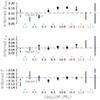 |
Fig. 7. Fit parameters for the Gaussian and exponential distributions plotted with increasing host galaxy mass. Alongside each parameter, the mean fit values is plotted in dash-dotted line to provide context. The fit results from the conservative sample are overlaid with triangles for comparison. See Sect. 4.2 for more details. |
Goodness-of-fit χ2 values for each parameter compared to the null hypothesis of no stellar mass evolution, with 9 DOF.
On the other hand, the EDust parameter displays a clear evolution, namely, > 6σ, with the mass of the host galaxy. The EDust values peak around the host galaxy mass of 10 /MStar, decreasing beyond this point for both higher and lower mass galaxies. The first mass bin, however, does not follow this trend. This does not appear to be a binning effect, as it persists across different bin edges and sizes. However, the discrepancy here may be caused by the mis-association of host galaxies, or biases arising from too-faint hosts (Paulino-Afonso et al. 2022). This trend is equally strong with the conservative sample, at > 6σ.
For both the z and host galaxy mass evolution tests, we attempted to account for potential non-Ia contamination in the signal by making use of simulations from Popovic et al. (2024). While these simulations are only available for SDSS and PS1, they are a good test for any potential signal contaminant by representing the two surveys with the highest potential non-Ia contamination. We performed the redshift and host galaxy mass analysis twice: once with a simulated contamination and once with a pure-Ia sample. We applied the same PIa > 0.9 cut to the contaminated simulated sample as we did in the case of the real data to test any bias due to this additional cut. This is compared with the pure SNIa simulated sample. We find no significant difference ( < 0.5σ) in recovered results between the contaminated and un-contaminated samples.
4.3. Evolution of β with host galaxy mass
While the observed c distribution is a tracer of EDust, it does not provide strong constraints on the type or size of the dust particulates, conventionally denoted as Rv. Instead, Rv has been shown to be better tracked with supernova data by the colour-luminosity relationship, β (Brout & Scolnic 2021; Popovic et al. 2023; Johansson et al. 2021). Here, we investigate the evolution of β with the host galaxy mass to see if whether a change is present in the dust properties, alongside the observed changes in the columnar density.
Figure 8 shows the colour-luminosity relationship for seven mass bins across the fiducial sample. Again, we have fit α alongside our β and assumed a Flat ΛCDM cosmology in making these plots. We focus on the inset that shows the fitted β values for each mass bin. With the exception of the first bin, there exists a clear trend of decreasing β with increasing host galaxy mass. Considering the bins that are populated for all three redshift categories (‘full’, ‘low-z’, and ‘high-z’), we find evidence of a change in β with mass at the 3σ level, likely driven by the lowest mass bins. These results are in line with those of Popovic et al. (2023), Chen et al. (2022) and provide further hints of changing host-galaxy properties. We discuss the inclusion of the first bin in Sect. 5.
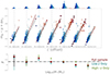 |
Fig. 8. Comparison of c vs. mB − μ + αx1, offset in bins of host galaxy mass, shown in the main plot. The SNe are colour-coded by their colour, c, for visual guidance. The slope (β value) for each mass bin is shown in red, alongside the fiducial beta in black dash-dotted line. The light grey dash-dotted vertical line shows the c = 0 point for each mass bin. Top: Colour histograms for each of the mass bins is shown, colour-coded according to c. Inset: β vs mass relationship for the fitted mass bins. The β values for the full sample are presented in brown points, the ZTF-only β values in teal triangle, and the high-redshift sample in olive triangle, with the fiducial β shown in grey dash-dotted line. See Sect. 4.3 for more details. |
5. Discussion
5.1. Redshift and mass evolution
We find no strong evidence for an evolving dust-free SNIa colour distribution with redshift. In our fiducial case, there are hints of the standard deviation of the dust-free distribution changing (3.4σ), but < 1σ evidence for the change in the mean of the dust-free distribution. Instead, we find very strong evidence of an evolving quantity of dust with redshift (> 6σ). Our conservative case finds no evidence for dust-free evolution and a weaker trend in dust evolution (3σ), although the weaker dust evolution trend is due to larger statistical uncertainties. However, the question of EDust evolution with the host galaxy mass becomes trickier. We have taken into consideration the exclusion of the first bin in our mass results; this is motivated by the potential of host galaxy mis-association at lower redshift. Our lowest mass bin at M < 8MStar is primarily dominated by low redshift galaxies; those galaxies at high redshift come with significant errors (on or above the order of 1MStar). If a SNIa was incorrectly associated to a lower mass host, it would effectively raise the observed EDust as a result of contamination from the true higher-mass hosts.
Rather than a linear model across the host galaxy stellar mass for EDust and β, it is possible that the 1010 mass bin represents a break-point for these parameters. For stellar masses above 1010, EDust is consistent with no evolution within 1.7σ; below this mass, the EDust parameter evolves with mass at a significance of 3.8σ. The opposite occurs with β: below a mass of 1010β does not change (< 1σ change from a flat line), compared to the familiar 3σ above 1010. In either case, these results hint at mass-dependent dust properties of SNe Ia.
This marks the first time that dust information with this fidelity has been extracted from SNIa light curves alone. With the exception of the aforementioned first bin, we find a continuous increase in the columnar density, EDust, to a peak and inflection point around 10MStar, followed by a decrease. This trend has been found in the literature, notably appearing in Zahid et al. (2013) and Calura et al. (2017). Zahid et al. (2013) finds an increasing extinction, AV, until an inflection point of 10MStar, whereby it decreases again. Interestingly, this behaviour holds for all star formation rates. Calura et al. (2017) shows increasing dust quantities with host galaxy mass, but only for large elliptical galaxies; spiral galaxies exhibit a flat relationship between mass and dust density. Rigault et al. (2020) proposes that this unique shape of the dust property evolution with mass is the byproduct of competing production modes: star formation rate (SFR) driven processes are responsible for increasing the amount of dust up until ≈1010 stellar masses, when star formation stops. Subsequently, explosion-processes driven by the large galactic stellar mass are the primary driver of dust relations for those galaxies heavier than ≈1010 stellar masses.
5.2. Evolution of β with redshift
The colour-luminosity coefficient β exhibits a strong linear relationship with the host galaxy stellar mass and this relationship holds regardless of redshift range. This follows the trends seen in Brout & Scolnic (2021) and Popovic et al. (2023), although those papers only fit in two bins of mass due to computational and statistical constraints, respectively. Previous analyses, such as those of Sullivan et al. (2010) and González-Gaitán et al. (2021), also reported evidence of multiple β values, but there was no evidence to support the notion that multiple β values alone could explain the ‘mass step’. Unlike González-Gaitán et al. (2021), we did not find any evidence of a sharp change in β at 10MStar. Instead, a continuous β relationship as a function of the host galaxy, Rv, remains the most probable explanation for this behaviour.
As a test to ensure that this behaviour of changing β with mass is not a sampling issue, we re-fit several downsampled instances of the full data set to check potential biases on β. We did not find significant biases on β (< 2σ) for samples as small as ×20 smaller than our full data.
In addition, we tested the evolution of β with redshift, defining
where β0 is the familiar SALT β value and β1 is the redshift-dependent term. We find β0 = 3.25, but no strong evidence for β evolution: β1 = 0.3 ± 0.4.
We note that earlier eras of cosmological analysis, such as JLA (Betoule et al. 2014), were dominated by systematic uncertainties arising from calibration. Today, analyses such as Popovic et al. (2024), Vincenzi et al. (2024) find that astrophysical processes not captured by light curve fitting methods are the driving force of systematic uncertainties. The results of this paper show strong evidence that the density of dust, either around the site of SNIa explosions, or within the galaxy as a whole, changes with redshift. This effect is degenerate with cosmology. The improper treatment of these effects in any cosmological analysis will preclude an accurate assessment of cosmological parameters.
6. Conclusion
In this paper, we have assembled a sample of ≈3000 SNIas that are free from magnitude-based selection effects, compiled from ZTF, SDSS, PS1, and DES. This selection marks the largest compilation of SNIa light curves to date, demonstrating the power of the ZTF sample.
With our ‘volume-limited’ sample and its more conservative counterpart, we have shown strong evidence for evolving host-galaxy properties. The amount of columnar dust density, EDust, changes significantly with both redshift z and the host galaxy mass. This contrasts with the lack of strong evidence for a change in the dust-free SNIa colour distribution, which is found to be well characterised by a Gaussian distribution in this work.
These results stand independent of potential non-Ia contamination, which we find to be mitigated by the placement of a Ia-probability cut on the data and our results persist for the conservative sample, providing strong evidence that these results are not a byproduct of magnitude-limited selection effects.
Additionally, we found evidence of a continuous and linear relationship between the colour-luminosity coefficient β and the host galaxy stellar mass, MStar. Taken altogether, these results point towards further proof that future standardisation modes for SNIa light curves must account for the properties of the host galaxy and that SNe Ia are becoming useful tools for extracting the dust properties of their host galaxies.
Acknowledgments
Based on observations obtained with the Samuel Oschin Telescope 48-inch and the 60-inch Telescope at the Palomar Observatory as part of the Zwicky Transient Facility project. ZTF is supported by the National Science Foundation under Grants No. AST-1440341 and AST-2034437 and a collaboration including current partners Caltech, IPAC, the Weizmann Institute of Science, the Oskar Klein Center at Stockholm University, the University of Maryland, Deutsches Elektronen-Synchrotron and Humboldt University, the TANGO Consortium of Taiwan, the University of Wisconsin at Milwaukee, Trinity College Dublin, Lawrence Livermore National Laboratories, IN2P3, University of Warwick, Ruhr University Bochum, Northwestern University and former partners the University of Washington, Los Alamos National Laboratories, and Lawrence Berkeley National Laboratories. Operations are conducted by COO, IPAC, and UW. SED Machine is based upon work supported by the National Science Foundation under Grant No. 1106171 The ZTF forced-photometry service was funded under the Heising-Simons Foundation grant #12540303 (PI: Graham). This project has received funding from the European Research Council (ERC) under the European Union’s Horizon 2020 research and innovation programme (grant agreement n°759194 – USNAC). This work has been supported by the Agence Nationale de la Recherche of the French government through the programme ANR-21-CE31-0016-03. Y.-L.K. has received funding from the Science and Technology Facilities Council [grant number ST/V000713/1]. This work has been supported by the research project grant “Understanding the Dynamic Universe” funded by the Knut and Alice Wallenberg Foundation under Dnr KAW 2018.0067, Vetenskapsrådet, the Swedish Research Council, project 2020-03444. L.G., T.E.M.B acknowledges financial support from the Spanish Ministerio de Ciencia e Innovación (MCIN) and the Agencia Estatal de Investigación (AEI) 10.13039/501100011033 under the PID2020-115253GA-I00 HOSTFLOWS project, from Centro Superior de Investigaciones Científicas (CSIC) under the PIE project 20215AT016 and the programme Unidad de Excelencia María de Maeztu CEX2020-001058-M, and from the Departament de Recerca i Universitats de la Generalitat de Catalunya through the 2021-SGR-01270 grant. Y.-L.K. has received funding from the Science and Technology Facilities Council [grant number ST/V000713/1]. UB, GD, JHT are supported by the H2020 European Research Council grant no. 758638.
References
- Amanullah, R., Lidman, C., Rubin, D., et al. 2010, ApJ, 716, 712 [CrossRef] [Google Scholar]
- Bellm, E. C., Kulkarni, S. R., Graham, M. J., et al. 2019, PASP, 131, 018002 [Google Scholar]
- Betoule, M., Kessler, R., Guy, J., et al. 2014, A&A, 568, A22 [NASA ADS] [CrossRef] [EDP Sciences] [Google Scholar]
- Blagorodnova, N., Neill, J. D., Walters, R., et al. 2018, PASP, 130, 035003 [Google Scholar]
- Briday, M., Rigault, M., Graziani, R., et al. 2022, A&A, 657, A22 [NASA ADS] [CrossRef] [EDP Sciences] [Google Scholar]
- Brout, D., & Scolnic, D. 2021, ApJ, 909, 26 [NASA ADS] [CrossRef] [Google Scholar]
- Brout, D., Scolnic, D., Popovic, B., et al. 2022, ApJ, 938, 110 [NASA ADS] [CrossRef] [Google Scholar]
- Calura, F., Pozzi, F., Cresci, G., et al. 2017, MNRAS, 465, 54 [Google Scholar]
- Chambers, K. C., Magnier, E. A., Metcalfe, N., et al. 2016, ArXiv e-prints [arXiv:1612.05560] [Google Scholar]
- Chen, R., Scolnic, D., Rozo, E., et al. 2022, ApJ, 938, 62 [NASA ADS] [CrossRef] [Google Scholar]
- Childress, M., Aldering, G., Antilogus, P., et al. 2013, ApJ, 770, 108 [Google Scholar]
- Childress, M. J., Wolf, C., & Zahid, H. J. 2014, MNRAS, 445, 1898 [Google Scholar]
- DESI Collaboration (Adame, A. G., et al.) 2024, ArXiv e-prints [arXiv:2404.03002] [Google Scholar]
- Foley, R. J., Scolnic, D., Rest, A., et al. 2018, MNRAS, 475, 193 [Google Scholar]
- Frieman, J. A., Bassett, B., Becker, A., et al. 2008, AJ, 135, 338 [Google Scholar]
- Ginolin, M., Rigault, M., Copin, Y., et al. 2025, A&A, 694, A4 (ZTF DR2 SI) [NASA ADS] [CrossRef] [EDP Sciences] [Google Scholar]
- González-Gaitán, S., de Jaeger, T., Galbany, L., et al. 2021, MNRAS, 508, 4656 [CrossRef] [Google Scholar]
- Graham, M. J., Kulkarni, S. R., Bellm, E. C., et al. 2019, PASP, 131, 078001 [Google Scholar]
- Guy, J., Sullivan, M., Conley, A., et al. 2010, A&A, 523, A7 [NASA ADS] [CrossRef] [EDP Sciences] [Google Scholar]
- Hamuy, M., Phillips, M. M., Suntzeff, N. B., et al. 1996, AJ, 112, 2391 [Google Scholar]
- Hicken, M., Challis, P., Jha, S., et al. 2009, ApJ, 700, 331 [Google Scholar]
- Howell, D. A., Sullivan, M., Conley, A., & Carlberg, R. 2007, ApJ, 667, L37 [NASA ADS] [CrossRef] [Google Scholar]
- James, F., & Roos, M. 1975, Comput. Phys. Commun., 10, 343 [Google Scholar]
- Johansson, J., Cenko, S. B., Fox, O. D., et al. 2021, ApJ, 923, 237 [NASA ADS] [CrossRef] [Google Scholar]
- Jones, D. O., Riess, A. G., Scolnic, D. M., et al. 2018, ApJ, 867, 108 [NASA ADS] [CrossRef] [Google Scholar]
- Kelly, P. L., Hicken, M., Burke, D. L., Mandel, K. S., & Kirshner, R. P. 2010, ApJ, 715, 743 [Google Scholar]
- Kelsey, L., Sullivan, M., Wiseman, P., et al. 2023, MNRAS, 519, 3046 [Google Scholar]
- Kessler, R., & Scolnic, D. 2017, ApJ, 836, 56 [Google Scholar]
- Krisciunas, K., Contreras, C., Burns, C. R., et al. 2017, AJ, 154, 211 [NASA ADS] [CrossRef] [Google Scholar]
- Kroupa, P. 2001, MNRAS, 322, 231 [NASA ADS] [CrossRef] [Google Scholar]
- Lampeitl, H., Smith, M., Nichol, R. C., et al. 2010, ApJ, 722, 566 [Google Scholar]
- Mandel, K. S., Scolnic, D. M., Shariff, H., Foley, R. J., & Kirshner, R. P. 2017, ApJ, 842, 93 [NASA ADS] [CrossRef] [Google Scholar]
- Masci, F. J., Laher, R. R., Rusholme, B., et al. 2019, PASP, 131, 018003 [Google Scholar]
- Möller, A., & de Boissière, T. 2020, MNRAS, 491, 4277 [CrossRef] [Google Scholar]
- Nicolas, N., Rigault, M., Copin, Y., et al. 2021, A&A, 649, A74 [NASA ADS] [CrossRef] [EDP Sciences] [Google Scholar]
- Paulino-Afonso, A., González-Gaitán, S., Galbany, L., et al. 2022, A&A, 662, A86 [NASA ADS] [CrossRef] [EDP Sciences] [Google Scholar]
- Perlmutter, S., Aldering, G., Goldhaber, G., et al. 1999, ApJ, 517, 565 [Google Scholar]
- Popovic, B., Scolnic, D., & Kessler, R. 2020, ApJ, 890, 172 [NASA ADS] [CrossRef] [Google Scholar]
- Popovic, B., Brout, D., Kessler, R., Scolnic, D., & Lu, L. 2021, ApJ, 913, 49 [NASA ADS] [CrossRef] [Google Scholar]
- Popovic, B., Brout, D., Kessler, R., & Scolnic, D. 2023, ApJ, 945, 84 [NASA ADS] [CrossRef] [Google Scholar]
- Popovic, B., Scolnic, D., Vincenzi, M., et al. 2024, MNRAS, 529, 2100 [CrossRef] [Google Scholar]
- Riess, A. G., Filippenko, A. V., Challis, P., et al. 1998, AJ, 116, 1009 [Google Scholar]
- Rigault, M., Copin, Y., Aldering, G., et al. 2013, A&A, 560, A66 [NASA ADS] [CrossRef] [EDP Sciences] [Google Scholar]
- Rigault, M., Neill, J. D., Blagorodnova, N., et al. 2019, A&A, 627, A115 [NASA ADS] [CrossRef] [EDP Sciences] [Google Scholar]
- Rigault, M., Brinnel, V., Aldering, G., et al. 2020, A&A, 644, A176 [NASA ADS] [CrossRef] [EDP Sciences] [Google Scholar]
- Sako, M., Bassett, B., Becker, A. C., et al. 2018, PASP, 130, 064002 [NASA ADS] [CrossRef] [Google Scholar]
- Sánchez, B. O., Brout, D., Vincenzi, M., et al. 2024, arXiv e-prints [arXiv:2406.05046] [Google Scholar]
- Scolnic, D., Kessler, R., Brout, D., et al. 2018, ApJ, 852, L3 [NASA ADS] [CrossRef] [Google Scholar]
- Smith, M., Sullivan, M., Wiseman, P., et al. 2020, MNRAS, 494, 4426 [Google Scholar]
- Sullivan, M., Le Borgne, D., Pritchet, C. J., et al. 2006, ApJ, 648, 868 [NASA ADS] [CrossRef] [Google Scholar]
- Sullivan, M., Conley, A., Howell, D. A., et al. 2010, MNRAS, 406, 782 [NASA ADS] [Google Scholar]
- Taylor, G., Lidman, C., Tucker, B. E., et al. 2021, MNRAS, 504, 4111 [NASA ADS] [CrossRef] [Google Scholar]
- Tripp, R. 1998, A&A, 331, 815 [NASA ADS] [Google Scholar]
- Uddin, S. A., Mould, J., Lidman, C., Ruhlmann-Kleider, V., & Zhang, B. R. 2017, ApJ, 848, 56 [CrossRef] [Google Scholar]
- Vincenzi, M., Brout, D., Armstrong, P., et al. 2024, ApJ, submitted [arXiv:2401.02945] [Google Scholar]
- Wiseman, P., Vincenzi, M., Sullivan, M., et al. 2022, MNRAS, 515, 4587 [NASA ADS] [CrossRef] [Google Scholar]
- Zahid, H. J., Yates, R. M., Kewley, L. J., & Kudritzki, R. P. 2013, ApJ, 763, 92 [NASA ADS] [CrossRef] [Google Scholar]
All Tables
Summary of redshift cuts for fiducial (Fid) and conservative (Con) samples after other quality cuts.
Goodness-of-fit χ2 values for each parameter compared to the null hypothesis of no z-evolution, with seven DOF.
Goodness-of-fit χ2 values for each parameter compared to the null hypothesis of no stellar mass evolution, with 9 DOF.
All Figures
|
Fig. 1. Redshift distributions for ZTF, SDSS, PS1, and DES. The full sample is presented for each survey before any redshift cuts in unfilled histogram. The light fill represents the redshift range of the fiducial sample and the dark fill shows the redshift range of the conservative sample. For details, see Sect. 2. |
| In the text | |
|
Fig. 2. mB vs. redshift for the SNIa in the Fiducial Sample defined in Table 1. Each supernova is colour coded according to its colour c. The grey vertical lines demark the quantile redshift bins, and the colour histogram is provided for each redshift bin in the inset plot. See Sect. 2 for more details. |
| In the text | |
|
Fig. 3. Fit results for the quantile redshift bins of the fiducial sample. The c distribution is shown for each redshift bin and colour coded to become darker with increasing redshift. For details, see Sect. 4.1. |
| In the text | |
|
Fig. 4. Fit parameters for the Gaussian and exponential distributions plotted with increasing redshift. Alongside each parameter, the mean fit value is plotted in dash-dotted line to provide context. The fit results from the conservative sample are overlaid in triangles for comparison. See more in Sect. 4.1. |
| In the text | |
|
Fig. 5. Host galaxy mass plotted vs redshift for the Fiducial sample. Supernovae are shown in grey, the coloured circles represent the median host galaxy mass in each quantile redshift bin. The dash-dotted black line shows the median host galaxy mass of the entire sample. The mass distribution, marginalised over redshift, is shown on the right. See Sect. 4.2 for more details. |
| In the text | |
|
Fig. 6. Fit results for the host galaxy mass bins of the fiducial sample. The c distribution is shown for each mass bin, colour coded with increasing host galaxy mass. (Sect. 4.2). |
| In the text | |
|
Fig. 7. Fit parameters for the Gaussian and exponential distributions plotted with increasing host galaxy mass. Alongside each parameter, the mean fit values is plotted in dash-dotted line to provide context. The fit results from the conservative sample are overlaid with triangles for comparison. See Sect. 4.2 for more details. |
| In the text | |
|
Fig. 8. Comparison of c vs. mB − μ + αx1, offset in bins of host galaxy mass, shown in the main plot. The SNe are colour-coded by their colour, c, for visual guidance. The slope (β value) for each mass bin is shown in red, alongside the fiducial beta in black dash-dotted line. The light grey dash-dotted vertical line shows the c = 0 point for each mass bin. Top: Colour histograms for each of the mass bins is shown, colour-coded according to c. Inset: β vs mass relationship for the fitted mass bins. The β values for the full sample are presented in brown points, the ZTF-only β values in teal triangle, and the high-redshift sample in olive triangle, with the fiducial β shown in grey dash-dotted line. See Sect. 4.3 for more details. |
| In the text | |
Current usage metrics show cumulative count of Article Views (full-text article views including HTML views, PDF and ePub downloads, according to the available data) and Abstracts Views on Vision4Press platform.
Data correspond to usage on the plateform after 2015. The current usage metrics is available 48-96 hours after online publication and is updated daily on week days.
Initial download of the metrics may take a while.