


| Issue |
A&A
Volume 711, July 2026
Euclid Quick Data Release (Q1)
|
|
|---|---|---|
| Article Number | A24 | |
| Number of page(s) | 21 | |
| Section | Extragalactic astronomy | |
| DOI | https://doi.org/10.1051/0004-6361/202554537 | |
| Published online | 30 June 2026 | |
Euclid Quick Data Release (Q1)
XXIV. Extending the quest for little red dots to z < 4
1
INAF-Osservatorio Astronomico di Padova, Via dell’Osservatorio 5, 35122 Padova, Italy
2
Dipartimento di Fisica e Astronomia “G. Galilei”, Università di Padova, Via Marzolo 8, 35131 Padova, Italy
3
School of Physics, HH Wills Physics Laboratory, University of Bristol, Tyndall Avenue, Bristol BS8 1TL, UK
4
Department of Mathematics and Physics, Roma Tre University, Via della Vasca Navale 84, 00146 Rome, Italy
5
INAF-Osservatorio Astronomico di Roma, Via Frascati 33, 00078 Monteporzio Catone, Italy
6
Max-Planck-Institut für Astronomie, Königstuhl 17, 69117 Heidelberg, Germany
7
INAF-Osservatorio Astrofisico di Arcetri, Largo E. Fermi 5, 50125 Firenze, Italy
8
INAF-Osservatorio Astronomico di Capodimonte, Via Moiariello 16, 80131 Napoli, Italy
9
School of Physics & Astronomy, University of Southampton, Highfield Campus, Southampton SO17 1BJ, UK
10
Jeremiah Horrocks Institute, University of Central Lancashire, Preston PR1 2HE, UK
11
Dipartimento di Fisica e Astronomia “G. Galilei”, Università di Padova, Vicolo dell’Osservatorio 3, 35122 Padova, Italy
12
INAF, Istituto di Radioastronomia, Via Piero Gobetti 101, 40129 Bologna, Italy
13
Institute of Cosmology and Gravitation, University of Portsmouth, Portsmouth PO1 3FX, UK
14
Cavendish Laboratory, University of Cambridge, JJ Thomson Avenue, Cambridge CB3 0HE, UK
15
Institute of Space Sciences (ICE, CSIC), Campus UAB, Carrer de Can Magrans, s/n, 08193 Barcelona, Spain
16
Institut d’Estudis Espacials de Catalunya (IEEC), Edifici RDIT, Campus UPC, 08860 Castelldefels, Barcelona, Spain
17
Max Planck Institute for Extraterrestrial Physics, Giessenbachstr. 1, 85748 Garching, Germany
18
Instituto de Astrofísica de Canarias (IAC); Departamento de Astrofísica, Universidad de La Laguna (ULL), 38200 La Laguna, Tenerife, Spain
19
Department of Astronomy, University of Geneva, ch. d’Ecogia 16, 1290 Versoix, Switzerland
20
Department of Physical Sciences, Ritsumeikan University, Kusatsu, Shiga, 525-8577, Japan
21
National Astronomical Observatory of Japan, 2-21-1 Osawa, Mitaka, Tokyo, 181-8588, Japan
22
Academia Sinica Institute of Astronomy and Astrophysics (ASIAA), 11F of ASMAB, No. 1, Section 4, Roosevelt Road, Taipei 10617, Taiwan
23
SRON Netherlands Institute for Space Research, Landleven 12, 9747 AD, Groningen, The Netherlands
24
Kapteyn Astronomical Institute, University of Groningen, PO Box 800, 9700 AV, Groningen, The Netherlands
25
INAF-Osservatorio di Astrofisica e Scienza dello Spazio di Bologna, Via Piero Gobetti 93/3, 40129 Bologna, Italy
26
Sterrenkundig Observatorium, Universiteit Gent, Krijgslaan 281 S9, 9000 Gent, Belgium
27
STAR Institute, University of Liège, Quartier Agora, Allée du six Août 19c, 4000 Liège, Belgium
28
INAF-Istituto di Astrofisica e Planetologia Spaziali, Via del Fosso del Cavaliere, 100, 00100 Roma, Italy
29
Dipartimento di Fisica e Astronomia “Augusto Righi” – Alma Mater Studiorum Università di Bologna, Via Piero Gobetti 93/2, 40129 Bologna, Italy
30
Université Paris-Saclay, CNRS, Institut d’astrophysique spatiale, 91405 Orsay, France
31
ESAC/ESA, Camino Bajo del Castillo, s/n., Urb. Villafranca del Castillo, 28692 Villanueva de la Cañada, Madrid, Spain
32
School of Mathematics and Physics, University of Surrey, Guildford, Surrey, GU2 7XH, UK
33
INAF-Osservatorio Astronomico di Brera, Via Brera 28, 20122 Milano, Italy
34
Université Paris-Saclay, Université Paris Cité, CEA, CNRS, AIM, 91191 Gif-sur-Yvette, France
35
IFPU, Institute for Fundamental Physics of the Universe, Via Beirut 2, 34151 Trieste, Italy
36
INAF-Osservatorio Astronomico di Trieste, Via G. B. Tiepolo 11, 34143 Trieste, Italy
37
INFN, Sezione di Trieste, Via Valerio 2, 34127 Trieste TS, Italy
38
SISSA, International School for Advanced Studies, Via Bonomea 265, 34136 Trieste TS, Italy
39
Dipartimento di Fisica e Astronomia, Università di Bologna, Via Gobetti 93/2, 40129 Bologna, Italy
40
INFN-Sezione di Bologna, Viale Berti Pichat 6/2, 40127 Bologna, Italy
41
Centre National d’Etudes Spatiales – Centre spatial de Toulouse, 18 avenue Edouard Belin, 31401 Toulouse Cedex 9, France
42
Universitäts-Sternwarte München, Fakultät für Physik, Ludwig-Maximilians-Universitäts-München, Scheinerstrasse 1, 81679 München, Germany
43
Space Science Data Center, Italian Space Agency, Via del Politecnico snc, 00133 Roma, Italy
44
Dipartimento di Fisica, Università di Genova, Via Dodecaneso 33, 16146 Genova, Italy
45
INFN-Sezione di Genova, Via Dodecaneso 33, 16146 Genova, Italy
46
Department of Physics “E. Pancini”, University Federico II, Via Cinthia 6, 80126 Napoli, Italy
47
Instituto de Astrofísica e Ciências do Espaço, Universidade do Porto, CAUP, Rua das Estrelas, PT4150-762 Porto, Portugal
48
Faculdade de Ciências da Universidade do Porto, Rua do Campo de Alegre, 4150-007 Porto, Portugal
49
Dipartimento di Fisica, Università degli Studi di Torino, Via P. Giuria 1, 10125 Torino, Italy
50
INFN-Sezione di Torino, Via P. Giuria 1, 10125 Torino, Italy
51
INAF-Osservatorio Astrofisico di Torino, Via Osservatorio 20, 10025 Pino Torinese (TO), Italy
52
European Space Agency/ESTEC, Keplerlaan 1, 2201 AZ, Noordwijk, The Netherlands
53
Institute Lorentz, Leiden University, Niels Bohrweg 2, 2333 CA, Leiden, The Netherlands
54
Leiden Observatory, Leiden University, Einsteinweg 55, 2333 CC, Leiden, The Netherlands
55
INAF-IASF Milano, Via Alfonso Corti 12, 20133 Milano, Italy
56
Centro de Investigaciones Energéticas, Medioambientales y Tecnológicas (CIEMAT), Avenida Complutense 40, 28040 Madrid, Spain
57
Port d’Informació Científica, Campus UAB, C. Albareda s/n, 08193 Bellaterra (Barcelona), Spain
58
Institute for Theoretical Particle Physics and Cosmology (TTK), RWTH Aachen University, 52056 Aachen, Germany
59
INFN section of Naples, Via Cinthia 6, 80126 Napoli, Italy
60
Institute for Astronomy, University of Hawaii, 2680 Woodlawn Drive, Honolulu HI 96822, USA
61
Dipartimento di Fisica e Astronomia “Augusto Righi” – Alma Mater Studiorum Università di Bologna, Viale Berti Pichat 6/2, 40127 Bologna, Italy
62
Instituto de Astrofísica de Canarias, Vía Láctea, 38205 La Laguna, Tenerife, Spain
63
Institute for Astronomy, University of Edinburgh, Royal Observatory, Blackford Hill, Edinburgh EH9 3HJ, UK
64
Jodrell Bank Centre for Astrophysics, Department of Physics and Astronomy, University of Manchester, Oxford Road, Manchester M13 9PL, UK
65
European Space Agency/ESRIN, Largo Galileo Galilei 1, 00044 Frascati, Roma, Italy
66
Université Claude Bernard Lyon 1, CNRS/IN2P3, IP2I Lyon, UMR 5822, Villeurbanne F-69100, France
67
Institut de Ciències del Cosmos (ICCUB), Universitat de Barcelona (IEEC-UB), Martí i Franquès 1, 08028 Barcelona, Spain
68
Institució Catalana de Recerca i Estudis Avançats (ICREA), Passeig de Lluís Companys 23, 08010 Barcelona, Spain
69
UCB Lyon 1, CNRS/IN2P3, IUF, IP2I Lyon, 4 rue Enrico Fermi, 69622 Villeurbanne, France
70
Mullard Space Science Laboratory, University College London, Holmbury St Mary, Dorking, Surrey, RH5 6NT, UK
71
Departamento de Física, Faculdade de Ciências, Universidade de Lisboa, Edifício C8, Campo Grande, PT1749-016 Lisboa, Portugal
72
Instituto de Astrofísica e Ciências do Espaço, Faculdade de Ciências, Universidade de Lisboa, Campo Grande, 1749-016 Lisboa, Portugal
73
INFN-Padova, Via Marzolo 8, 35131 Padova, Italy
74
Aix-Marseille Université, CNRS/IN2P3, CPPM, Marseille, France
75
INFN-Bologna, Via Irnerio 46, 40126 Bologna, Italy
76
FRACTAL S.L.N.E., calle Tulipán 2, Portal 13 1A, 28231 Las Rozas de Madrid, Spain
77
NRC Herzberg, 5071 West Saanich Rd, Victoria BC V9E 2E7, Canada
78
Institute of Theoretical Astrophysics, University of Oslo, P.O. Box 1029 Blindern, 0315 Oslo, Norway
79
Jet Propulsion Laboratory, California Institute of Technology, 4800 Oak Grove Drive, Pasadena, CA, 91109, USA
80
Department of Physics, Lancaster University, Lancaster LA1 4YB, UK
81
Felix Hormuth Engineering, Goethestr. 17, 69181 Leimen, Germany
82
Technical University of Denmark, Elektrovej 327, 2800 Kgs. Lyngby, Denmark
83
Cosmic Dawn Center (DAWN), Denmark
84
Institut d’Astrophysique de Paris, UMR 7095, CNRS, and Sorbonne Université, 98 bis boulevard Arago, 75014 Paris, France
85
NASA Goddard Space Flight Center, Greenbelt MD 20771, USA
86
Department of Physics and Helsinki Institute of Physics, Gustaf Hällströmin katu 2, 00014 University of Helsinki, Finland
87
Université de Genève, Département de Physique Théorique and Centre for Astroparticle Physics, 24 quai Ernest-Ansermet, CH-1211 Genève 4, Switzerland
88
Department of Physics, P.O. Box 64, 00014 University of Helsinki, Finland
89
Helsinki Institute of Physics, Gustaf Hällströmin katu 2, University of Helsinki, Helsinki, Finland
90
Centre de Calcul de l’IN2P3/CNRS, 21 avenue Pierre de Coubertin, 69627 Villeurbanne Cedex, France
91
Laboratoire d’etude de l’Univers et des phenomenes eXtremes, Observatoire de Paris, Université PSL, Sorbonne Université, CNRS, 92190 Meudon, France
92
Aix-Marseille Université, CNRS, CNES, LAM, Marseille, France
93
SKA Observatory, Jodrell Bank, Lower Withington, Macclesfield, Cheshire SK11 9FT, UK
94
Dipartimento di Fisica “Aldo Pontremoli”, Università degli Studi di Milano, Via Celoria 16, 20133 Milano, Italy
95
INFN-Sezione di Milano, Via Celoria 16, 20133 Milano, Italy
96
University of Applied Sciences and Arts of Northwestern Switzerland, School of Computer Science, 5210 Windisch, Switzerland
97
Universität Bonn, Argelander-Institut für Astronomie, Auf dem Hügel 71, 53121 Bonn, Germany
98
INFN-Sezione di Roma, Piazzale Aldo Moro, 2 – c/o Dipartimento di Fisica, Edificio G. Marconi, 00185 Roma, Italy
99
Department of Physics, Institute for Computational Cosmology, Durham University, South Road, Durham DH1 3LE, UK
100
Université Côte d’Azur, Observatoire de la Côte d’Azur, CNRS, Laboratoire Lagrange, Bd de l’Observatoire, CS 34229, 06304 Nice cedex 4, France
101
Université Paris Cité, CNRS, Astroparticule et Cosmologie, 75013 Paris, France
102
CNRS-UCB International Research Laboratory, Centre Pierre Binetruy, IRL2007, CPB-IN2P3, Berkeley, USA
103
University of Applied Sciences and Arts of Northwestern Switzerland, School of Engineering, 5210 Windisch, Switzerland
104
Institut d’Astrophysique de Paris, 98bis Boulevard Arago, 75014 Paris, France
105
Institute of Physics, Laboratory of Astrophysics, Ecole Polytechnique Fédérale de Lausanne (EPFL), Observatoire de Sauverny, 1290 Versoix, Switzerland
106
Aurora Technology for European Space Agency (ESA), Camino bajo del Castillo, s/n, Urbanizacion Villafranca del Castillo, Villanueva de la Cañada, 28692 Madrid, Spain
107
Institut de Física d’Altes Energies (IFAE), The Barcelona Institute of Science and Technology, Campus UAB, 08193 Bellaterra (Barcelona), Spain
108
School of Mathematics, Statistics and Physics, Newcastle University, Herschel Building, Newcastle-upon-Tyne, NE1 7RU, UK
109
DARK, Niels Bohr Institute, University of Copenhagen, Jagtvej 155, 2200 Copenhagen, Denmark
110
Waterloo Centre for Astrophysics, University of Waterloo, Waterloo, Ontario, N2L 3G1, Canada
111
Department of Physics and Astronomy, University of Waterloo, Waterloo, Ontario, N2L 3G1, Canada
112
Perimeter Institute for Theoretical Physics, Waterloo, Ontario, N2L 2Y5, Canada
113
Institute of Space Science, Str. Atomistilor, nr. 409Măgurele, Ilfov 077125, Romania
114
Consejo Superior de Investigaciones Cientificas, Calle Serrano 117, 28006 Madrid, Spain
115
Universidad de La Laguna, Departamento de Astrofísica, 38206 La Laguna, Tenerife, Spain
116
Caltech/IPAC, 1200 E. California Blvd., Pasadena, CA, 91125, USA
117
Institut für Theoretische Physik, University of Heidelberg, Philosophenweg 16, 69120 Heidelberg, Germany
118
Institut de Recherche en Astrophysique et Planétologie (IRAP), Université de Toulouse, CNRS, UPS, CNES, 14 Av. Edouard Belin, 31400 Toulouse, France
119
Université St Joseph; Faculty of Sciences, Beirut, Lebanon
120
Departamento de Física, FCFM, Universidad de Chile, Blanco Encalada 2008, Santiago, Chile
121
Universität Innsbruck, Institut für Astro- und Teilchenphysik, Technikerstr. 25/8, 6020 Innsbruck, Austria
122
Satlantis, University Science Park, Sede Bld 48940, Leioa-Bilbao, Spain
123
Infrared Processing and Analysis Center, California Institute of Technology, Pasadena, CA, 91125, USA
124
Instituto de Astrofísica e Ciências do Espaço, Faculdade de Ciências, Universidade de Lisboa, Tapada da Ajuda, 1349-018 Lisboa, Portugal
125
Cosmic Dawn Center (DAWN)
126
Niels Bohr Institute, University of Copenhagen, Jagtvej 128, 2200 Copenhagen, Denmark
127
Universidad Politécnica de Cartagena, Departamento de Electrónica y Tecnología de Computadoras, Plaza del Hospital 1, 30202 Cartagena, Spain
128
Dipartimento di Fisica e Scienze della Terra, Università degli Studi di Ferrara, Via Giuseppe Saragat 1, 44122 Ferrara, Italy
129
Istituto Nazionale di Fisica Nucleare, Sezione di Ferrara, Via Giuseppe Saragat 1, 44122 Ferrara, Italy
130
Department of Physics, Oxford University, Keble Road, Oxford OX1 3RH, UK
131
Université PSL, Observatoire de Paris, Sorbonne Université, CNRS, LERMA, 75014 Paris, France
132
Université Paris-Cité, 5 Rue Thomas Mann, 75013 Paris, France
133
Zentrum für Astronomie, Universität Heidelberg, Philosophenweg 12, 69120 Heidelberg, Germany
134
INAF-Osservatorio Astronomico di Brera, Via Brera 28, 20122 Milano, Italy, and INFN-Sezione di Genova, Via Dodecaneso 33, 16146 Genova, Italy
135
ICL, Junia, Université Catholique de Lille, LITL, 59000 Lille, France
136
ICSC – Centro Nazionale di Ricerca in High Performance Computing, Big Data e Quantum Computing, Via Magnanelli 2, Bologna, Italy
137
Instituto de Física Teórica UAM-CSIC, Campus de Cantoblanco, 28049 Madrid, Spain
138
CERCA/ISO, Department of Physics, Case Western Reserve University, 10900 Euclid Avenue, Cleveland OH 44106, USA
139
Technical University of Munich, TUM School of Natural Sciences, Physics Department, James-Franck-Str. 1, 85748 Garching, Germany
140
Max-Planck-Institut für Astrophysik, Karl-Schwarzschild-Str. 1, 85748 Garching, Germany
141
Laboratoire Univers et Théorie, Observatoire de Paris, Université PSL, Université Paris Citer, CNRS, 92190 Meudon, France
142
Departamento de Física Fundamental. Universidad de Salamanca., Plaza de la Merced s/n, 37008 Salamanca, Spain
143
Université de Strasbourg, CNRS, Observatoire astronomique de Strasbourg, UMR 7550, 67000 Strasbourg, France
144
Center for Data-Driven Discovery, Kavli IPMU (WPI), UTIAS, The University of Tokyo, Kashiwa, Chiba, 277-8583, Japan
145
California Institute of Technology, 1200 E California Blvd, Pasadena, CA, 91125, USA
146
Department of Physics & Astronomy, University of California Irvine, Irvine CA, 92697, USA
147
Department of Mathematics and Physics E. De Giorgi, University of Salento, Via per Arnesano, CP-I93, 73100 Lecce, Italy
148
INFN, Sezione di Lecce, Via per Arnesano, CP-193, 73100 Lecce, Italy
149
INAF-Sezione di Lecce, c/o Dipartimento Matematica e Fisica, Via per Arnesano, 73100 Lecce, Italy
150
Departamento Física Aplicada, Universidad Politécnica de Cartagena, Campus Muralla del Mar, 30202 Cartagena, Murcia, Spain
151
Instituto de Física de Cantabria, Edificio Juan Jordá, Avenida de los Castros, 39005 Santander, Spain
152
CEA Saclay, DFR/IRFU, Service d’Astrophysique, Bat. 709, 91191 Gif-sur-Yvette, France
153
Department of Computer Science, Aalto University, PO Box 15400 Espoo FI-00 076, Finland
154
Instituto de Astrofísica de Canarias, c/ Via Lactea s/n, La Laguna 38200, Spain. Departamento de Astrofísica de la Universidad de La Laguna, Avda. Francisco Sanchez, La Laguna, 38200, Spain
155
Ruhr University Bochum, Faculty of Physics and Astronomy, Astronomical Institute (AIRUB), German Centre for Cosmological Lensing (GCCL), 44780 Bochum, Germany
156
Department of Physics and Astronomy, Vesilinnantie 5, 20014 University of Turku, Finland
157
Serco for European Space Agency (ESA), Camino bajo del Castillo, s/n, Urbanizacion Villafranca del Castillo, Villanueva de la Cañada, 28692 Madrid, Spain
158
ARC Centre of Excellence for Dark Matter Particle Physics, Melbourne, Australia
159
Centre for Astrophysics & Supercomputing, Swinburne University of Technology, Hawthorn, Victoria, 3122, Australia
160
Department of Physics and Astronomy, University of the Western Cape, Bellville, Cape Town, 7535, South Africa
161
DAMTP, Centre for Mathematical Sciences, Wilberforce Road, Cambridge CB3 0WA, UK
162
Kavli Institute for Cosmology Cambridge, Madingley Road, Cambridge CB3 0HA, UK
163
Department of Astrophysics, University of Zurich, Winterthurerstrasse 190, 8057 Zurich, Switzerland
164
Department of Physics, Centre for Extragalactic Astronomy, Durham University, South Road, Durham DH1 3LE, UK
165
IRFU, CEA, Université Paris-Saclay, 91191 Gif-sur-Yvette Cedex, France
166
Oskar Klein Centre for Cosmoparticle Physics, Department of Physics, Stockholm University, Stockholm SE-106 91, Sweden
167
Astrophysics Group, Blackett Laboratory, Imperial College London, London SW7 2AZ, UK
168
Univ. Grenoble Alpes, CNRS, Grenoble INP, LPSC-IN2P3, 53, Avenue des Martyrs, 38000 Grenoble, France
169
Dipartimento di Fisica, Sapienza Università di Roma, Piazzale Aldo Moro 2, 00185 Roma, Italy
170
Centro de Astrofísica da Universidade do Porto, Rua das Estrelas, 4150-762 Porto, Portugal
171
HE Space for European Space Agency (ESA), Camino bajo del Castillo, s/n, Urbanizacion Villafranca del Castillo, Villanueva de la Cañada, 28692 Madrid, Spain
172
Dipartimento di Fisica – Sezione di Astronomia, Università di Trieste, Via Tiepolo 11, 34131 Trieste, Italy
173
Department of Astrophysical Sciences, Peyton Hall, Princeton University, Princeton NJ 08544, USA
174
Theoretical astrophysics, Department of Physics and Astronomy, Uppsala University, Box 515, 751 20 Uppsala, Sweden
175
Minnesota Institute for Astrophysics, University of Minnesota, 116 Church St SE, Minneapolis MN 55455, USA
176
Mathematical Institute, University of Leiden, Einsteinweg 55, 2333 CA, Leiden, The Netherlands
177
ASTRON, the Netherlands Institute for Radio Astronomy, Postbus 2, 7990 AA, Dwingeloo, The Netherlands
178
Center for Advanced Interdisciplinary Research, Ss. Cyril and Methodius University in Skopje, Macedonia
179
Institute of Astronomy, University of Cambridge, Madingley Road, Cambridge CB3 0HA, UK
180
Space physics and astronomy research unit, University of Oulu, Pentti Kaiteran katu 1, FI-90014 Oulu, Finland
181
Center for Computational Astrophysics, Flatiron Institute, 162 5th Avenue, 10010 New York, NY, USA
182
Department of Astronomy, University of Massachusetts, Amherst MA 01003, USA
183
Department of Physics and Astronomy, University of British Columbia, Vancouver BC V6T 1Z1, Canada
★ Corresponding author: This email address is being protected from spambots. You need JavaScript enabled to view it.
Received:
14
March
2025
Accepted:
19
July
2025
Abstract
Recent observations with the James Webb Space Telescope (JWST) have revealed an interesting population of sources with a compact morphology and a characteristic v-shaped continuum, namely blue at a rest frame λ < 4000 Å and red at longer wavelengths. The nature of these sources, which are called little red dots (LRDs), is still highly debated because it is unclear whether they host active galactic nuclei (AGNs) and their number seems to drop drastically at z < 4. We took advantage of the 63 deg2 covered by the Euclid Quick Data Release (Q1) to extend the search for LRDs to brighter magnitudes and lower redshifts than what was possible with JWST. This is fundamental for a broader view of the evolution of this peculiar galaxy population. The selection was performed by fitting the available photometric data (Euclid, the Spitzer Infrared Array Camera (IRAC), and ground-based griz data) with two power laws to retrieve the rest-frame optical and UV slopes consistently over a wide redshift range (i.e. z < 7.6). We then excluded extended objects and possible line emitters and inspected the data visually to remove any imaging artefacts. The final selection included 3341 LRD candidates from z = 0.33 to z = 3.6, 29 of which were also detected in IRAC. The resulting rest-frame UV luminosity function, in contrast with previous JWST studies, shows that the number density of LRD candidates increases from high redshift to z = 1.5–2.5 and decreases at even lower redshifts. The subsample of more robust LRD candidates that are also detected with IRAC show a weaker evolution, however, which is affected by low statistics and limited by the IRAC resolution. The comparison with previous quasar UV luminosity functions shows that LRDs are not the dominant AGN population at z < 4 and MUV < −21. Follow-up studies of these LRD candidates are pivotal to confirm their nature, probe their physical properties, and determine whether they are compatible with JWST sources because the different spatial resolution and wavelength coverage of Euclid and JWST might select different samples of compact sources.
Key words: galaxies: active / galaxies: evolution / galaxies: luminosity function / mass function
© The Authors 2026
 Open Access article, published by EDP Sciences, under the terms of the Creative Commons Attribution License (https://creativecommons.org/licenses/by/4.0), which permits unrestricted use, distribution, and reproduction in any medium, provided the original work is properly cited.
This article is published in open access under the Subscribe to Open model. This email address is being protected from spambots. You need JavaScript enabled to view it. to support open access publication.
1. Introduction
Supermassive black holes (SMBHs) with tens of millions of solar masses appear to be ubiquitous at the centres of local galaxies (e.g. Magorrian et al. 1998; Gültekin et al. 2009). Moreover, a close co-evolution that links SMBHs to their host galaxies is suggested by the tight scaling relations that are observed between the SMBH masses and different galactic properties (e.g. Magorrian et al. 1998; Silk & Rees 1998; Gebhardt et al. 2000; Ferrarese 2002; Mullaney et al. 2012; Delvecchio et al. 2022). Theoretical models calibrated against present-day scaling relations seem to produce a wide range of SMBH properties at higher redshifts, however, which arise from the differences in the implementation of supernova and BH feedback and sub-grid physics (e.g. Habouzit et al. 2020, 2021). It is therefore important to extend the analysis of SMBHs and their host galaxies to a wide range of times.
Observational evidence for massive accreting BHs that shine as active galactic nuclei (AGNs) at increasingly higher redshifts places strong constraints on their formation scenarios and the mass of their seeds. The formation of a 109 M⊙ SMBH by z = 7 requires a heavy seed (MBH ∼ 105 M⊙), a light seed (MBH ∼ 102 M⊙) that accretes for some time at super-Eddington or hyper-Eddington rates (e.g. Wyithe & Loeb 2012; Alexander & Natarajan 2014; Inayoshi et al. 2016; Begelman & Volonteri 2017; Pacucci et al. 2017; Pacucci & Loeb 2022; Maiolino et al. 2024a), or primordial BHs that formed as a result of fluctuations in the early Universe (Hawking 1971; Carr & Hawking 1974; Dayal et al. 2025). It is unclear, however, whether the currently observed high-z AGNs can be considered representative of the whole AGN population. The study of low-luminosity AGNs and low-mass SMBHs is therefore key to placing constraints on the mass distribution for seeds of high-z AGNs.
The epoch of reionisation marks the transition phase at which the first sources of ultraviolet (UV) radiation were able, after the so-called dark ages, to ionise hydrogen atoms in the surrounding intergalactic medium for the first time (Barkana & Loeb 2001; Dayal & Ferrara 2018). It is still largely debated which sources caused this process, however. Many studies identified low-mass metal-poor star-forming galaxies at high redshift as the main driver of cosmic reionisation (e.g. Atek et al. 2024; Simmonds et al. 2024; Dayal 2024), and others showed evidence that faint AGNs can contribute significantly to reionisation (e.g. Asthana et al. 2024) and in some cases dominate reionisation (e.g. Madau et al. 2024; Grazian et al. 2024). It is therefore fundamental to quantify the number density of these faint AGNs to constrain their contribution to the reionisation of the Universe.
The first years of observations with the James Webb Space Telescope (JWST) have revealed a new intriguing population of compact red sources that are characterised by a peculiar v-shaped spectral energy distribution (SED), namely a blue rest-frame UV continuum and a steep red slope in the rest-frame optical (e.g. Kocevski et al. 2023, 2025; Harikane et al. 2023; Matthee et al. 2024; Greene et al. 2024; Labbé et al. 2023; Labbe et al. 2025; Killi et al. 2024; Furtak et al. 2023). These so-called little red dots (LRDs) are mainly observed at z ≥ 4 and can easily be selected by photometric observations because their morphology is compact and their SED shape is peculiar. Particular care needs to be taken to remove contaminating populations, however, such as brown dwarfs, which correspond to 21% of the colour-selected JWST LRD candidates according to Langeroodi & Hjorth (2023).
The nature of these LRDs is heavily debated. Their steep rest-frame optical slopes are consistent with either a reddened AGN continuum or emission from dusty star formation (e.g. Kocevski et al. 2023; Barro et al. 2024a; Labbé et al. 2023; Akins et al. 2024), with evidence supporting both scenarios. For example, spectroscopic follow-up studies of LRDs have shown that about 80% of them show broad hydrogen (H α and H β) emission (e.g. Kocevski et al. 2023, 2025; Kokorev et al. 2024a; Killi et al. 2024; Matthee et al. 2024; Furtak et al. 2023; Greene et al. 2024; Wang et al. 2024), with general line widths with an FWHM ≤ 1000 km s−1, but some even reach 3000 km s−1. These line widths would far exceed those of typical star-forming galaxies at lower redshift (e.g. Fumagalli et al. 2012), which supports the AGN scenario. In this picture, we have a direct view of the broad-line region and the accretion disk of the AGN, but with foreground dust attenuation that either originates from a dusty interstellar medium (ISM) or from nuclear dust (see, e.g. Netzer 2015; Hickox & Alexander 2018). This scenario would mean that LRDs are similar to the red quasars that are observed at lower redshifts (e.g. Webster et al. 1995; Richards et al. 2003; Urrutia et al. 2008; Glikman et al. 2012, 2015), considering also that some of these red quasar show a similar excess of UV light (Wethers et al. 2018; Stepney et al. 2024). While the majority of LRDs may host an AGN, they represent a sub-sample of the overall AGN population. Out of the large number of broad-line AGNs discovered by JWST, only 10–30% have SEDs that are typical of LRDs (Hainline et al. 2025).
The SMBH masses inferred for these LRDs lie in the range MBH = 106–108 M⊙, and their stellar masses range from 107 to 1011 M⊙. This shows that a fraction of them are over-massive relative to the stellar masses of their host galaxies when compared to the local MBH–M* relation (e.g. Maiolino et al. 2024b; Harikane et al. 2023), and they are consistent with the local relation between MBH and stellar velocity dispersion (Maiolino et al. 2024b). This finding indicates they may be going through super-Eddington accretion or originate from heavy BH seeds. Bellovary (2025) instead recently hypothesised that LRDs might be runaway-collapse globular clusters with tidal disruption events, which might explain their compact size, UV luminosities, and high number densities.
In the scenario in which LRDs are entirely powered by dusty starbursts, they would correspond to very massive galaxies (M* = 109–1011 M⊙). In this picture, a final excess of massive early galaxies would be reached, but some of which would contradict cosmological models and some would be so compact as to be unstable against supernovae feedback (Wang et al. 2024; Akins et al. 2024). This supports the AGN scenario. Mid-infrared (mid-IR) observations at 5–25 μm have shown a remarkably flat continuum, however, which favours SED models consistent with a dusty compact starburst and only a mild contribution from an obscured AGN (Williams et al. 2024; Pérez-González et al. 2024) or an AGN torus without hot dust (Leung et al. 2024; Barro et al. 2024b). Only two LRDs have been detected in the far-IR so far, which provides some indications of warm dust emission (Barro et al. 2024b; Juodžbalis et al. 2024), and many other LRDs have not been detected in the far-IR. This limits the possible presence of cool or warm dust that is linked to star formation (Labbe et al. 2025). Moreover, the spectra of several broad-line objects show a clear Balmer break, which implies that evolved stars might indeed contribute to the rest-frame optical (Kokorev et al. 2024b). The precise contribution is highly degenerate, however (Wang et al. 2024).
In addition, the majority of LRDs are not strong X-ray emitters. They are undetected (or only marginally detected) even in very deep observations or in a stacking analysis (Ananna et al. 2024; Yue et al. 2024). For this reason, some studies have hypothesised that the broad-line components cannot be due to an AGN, but to outflows driven by star formation or inelastic Raman scattering of stellar UV continua by neutral hydrogen atoms (Kokubo & Harikane 2024). Alternatively, other studies have reported that the broadening might be consistent with the stellar velocity dispersion if the galaxy were going through a short-lived phase when the central densities are much higher than at later times (Baggen et al. 2024). Other studies have instead suggested that the X-ray weakness might be due to a very steep X-ray spectrum that is induced by the absorption by large Compton-thick columns or a very high BH accretion rate (Maiolino et al. 2025). The last two scenarios would also explain the non-detection at radio frequencies (Mazzolari et al. 2026). The dense neutral gas around the AGN accretion disk would also mimic a Balmer break, which indicates that the rest-frame optical may not be due to evolved stars (Inayoshi & Maiolino 2025). The absence of variability in the rest-frame UV, except for a few LRDs (Zhang et al. 2025), may argue against a strong contribution by AGN, however (Tee et al. 2025; Kokubo & Harikane 2024).
The uncertainties on the nature of the LRDs are, at least partially, driven by their high-z nature, which implies that they are faint and require near-IR observations. While preliminary studies trying to find low-z and local analogues have been performed by, for example, Noboriguchi et al. (2023), Mezcua et al. (2024), and Lin et al. (2025), large near-IR surveys are necessary to follow the redshift evolution of LRDs because their number density has been suggested to dramatically drop at z < 4 (Kocevski et al. 2025). Moreover, large near-IR surveys like this are key for probing the LRD clustering on large scales. Tanaka et al. (2024) already suggested that LRDs may show an excess of clustering at kiloparsec scales. The large observed area and the near-IR coverage of Euclid (Euclid Collaboration: Mellier et al. 2025) is therefore ideal to search for and study LRDs.
We searched for LRDs using the newly available Euclid Quick Release Q1 (2025), combined with publicly available images from the Spitzer Infrared Array Camera (IRAC) and ground-based optical data. The area and depth of these Euclid observations are ideal for a first characterisation of the bright end of the LRD luminosity function and to extend the search to z < 4. To select LRDs, we follow the approach by Kocevski et al. (2025) and select them using cuts on the rest-frame optical and UV slopes. The paper is structured as follows. In Sect. 2 we present a summary of the Euclid data products we used, as well as the ancillary IRAC images. In Sect. 3 we outline our selection method, and we discuss our findings in Sect. 4. The final conclusion and future prospects are reported in Sect. 5. Throughout the paper, we consider a ΛCDM cosmology with H0 = 70 km s−1 Mpc−1, Ωm = 0.27, and ΩΛ = 0.73. All magnitudes are reported in the AB system (Oke & Gunn 1983).
2. Data description
2.1. Euclid data products
The Q1 data release was described by Euclid Collaboration: Aussel et al. (2026), the Visible Camera (VIS) and Near-Infrared Spectrometer and Photometer (NISP) processing and data products were reported by Euclid Collaboration: McCracken et al. (2026) and Euclid Collaboration: Polenta et al. (2026), respectively, and the photometric catalogue was discussed in Euclid Collaboration: Romelli et al. (2026). An overview of the scientific objectives of the Euclid ESA mission was reported in Euclid Collaboration: Mellier et al. (2025).
Briefly, Q1 includes 63 deg2 of the extragalactic sky, divided into three fields: 22 deg2 in the Euclid Deep Field North (EDF-N); 12 deg2 in the Euclid Deep Field Fornax (EDF-F); and 28 deg2 in the Euclid Deep Field South (EDF-S). Each field has been observed in four photometric bands, one band in the visible (IE, Euclid Collaboration: Cropper et al. 2025), and three bands in the near-IR (NISP, YE, JE, and HE band, see Euclid Collaboration: Jahnke et al. 2025). In addition, these observations are complemented with ground-based observations that are carried out with multiple instruments and cover between 0.3 μm and 0.9 μm. They are part of the Ultraviolet Near-Infrared Optical Northern Survey (UNIONS; Gwyn et al., in prep.) or the Dark Energy Survey (Abbott et al. 2018). The complete list of available filters in each field and their corresponding observational depths are reported in Table 1.
Filters and associated observed depths.
We considered aperture photometry measured for all bands on the images convolved to the lowest spatial resolution (usually a ground-based band). We considered an aperture with a diameter of two full widths at half maximum (FWHM; a median value of  ), and we corrected it to the total (see Euclid Collaboration: Romelli et al. 2026, for more details). We also corrected each flux for Galactic extinction using the position of each source and the relation by Gordon et al. (2023), which strongly relies on the results by Gordon et al. (2009), Fitzpatrick et al. (2019), Gordon et al. (2021), and Decleir et al. (2022).
2.2. IRAC photometry
We started from the collection of IRAC images described by Euclid Collaboration: Moneti et al. (2022), which cover a fraction of the Euclid Deep Fields (EDFs) as part of the Cosmic Dawn survey (Euclid Collaboration: McPartland et al. 2025). The images result from a collection of different programmes with a non-uniform coverage in area and depth. We report the average 10σ depths in Table 1 and the area coverage in Table 2. The IRAC3 and IRAC4 filters are only available for a small portion of the EDF-F and EDF-N, and none is available for the EDF-S.
Area coverage in deg2 of the available IRAC images (Euclid Collaboration: Moneti et al. 2022).
Starting from the public images, we removed the sky background using the Python pacakge PHOTUTILS (Bradley et al. 2023). We derived the median value using a filter with 3 pixel × 3 pixels. With the same package, we then used the position of all Euclid sources to extract aperture photometry with an aperture radius of 1″, which is consistent with half the smallest FWHM of IRAC, from all available IRAC images. In this preliminary work, no attempt was made to de-blend IRAC sources using the Euclid positions. For this reason, we visually confirmed the selected LRD candidates to remove objects that were affected by blending.
To derive the correction for the aperture to the total fluxes for all four IRAC filters, we compared this catalogue with a separate extraction that was performed for the EDF-N alone (Bisigello et al. 2025). The extraction was performed using the co-added IRAC1 and IRAC2 images as the detection image, weighted for each uncertainty map, and considering Kron apertures that were derived with a scaling parameter of the unscaled Kron radius of 1.8 and a minimum value for the unscaled Kron radius of 2.5 pixels. We then matched the two EDF-N catalogues with the aperture and Kron fluxes to derive the aperture-to-total correction in each filter. We applied the same correction in all three fields.
We verified that the total fluxes were consistent with the catalogues described by Euclid Collaboration: Zalesky et al. (2025), which only cover two out of three EDFs, however, and only include the IRAC1 and IRAC2 filters. The comparison is shown in Appendix A. The magnitudes we derived are clearly brighter on average by 0.1 magnitudes in the EDF-F and by 0.3 magnitudes in the EDF-N than the magnitudes presented in the Cosmic Dawn Catalogue. The agreement is, however, within 0.1 magnitudes when we only consider bright objects (i.e. IRAC1 or IRAC2 < 21).
2.3. Photometric redshifts
As a first estimate of the photometric redshift, we considered the median value and the two first modes derived in the main Euclid pipeline, which were described in detail by Euclid Collaboration: Tucci et al. (2026). Because these estimates are limited to z = 6, we also considered the redshift estimate derived for NISP-detected objects. This extended the redshift range to z = 12. In this case, we considered the redshift of the highest peak of the probability distribution as the best estimate. As tested by Appendix B, the redshift estimation for LRDs derived from the pipeline includes about 40% of outliers because LRD templates are not included in the pipeline at the moment. We discuss the method we used to improve these estimates below.
3. Sample selection
Previous JWST photometric studies mainly identified LRDs by applying some colour cuts to compact sources (e.g. Barro et al. 2024a; Labbe et al. 2025; Kokorev et al. 2024a). This type of selection is difficult to apply directly to Euclid, however, because the filter set is different. In addition, a simple colour cut does not allow us to select the sources uniformly at different redshifts because it is based on observed and not on rest-frame properties. Therefore, we considered the alternative approach adopted by Kocevski et al. (2025) and selected sources with a compact morphology, a red continuum in the rest-frame optical wavelengths, and a blue continuum in the rest-frame UV. The latter two quantities were directly derived by fitting the available photometric data. We report the entire classification procedure we applied in detail below, and we report in Table 3 the original source number in each field and the change in this number at the different selection steps.
Number of sources retrieved in the different steps of the LRD selection in the three EDFs.
3.1. LRD selection procedure
As a first conservative selection, we removed objects that were classified as stars (PHZ_CLASSIFICATION = 1) using the classification from the PHZ processing function (Euclid Collaboration: Tucci et al. 2026). This classification is based on photometry and not on compactness. This is fundamental to avoid removing any LRD candidates. We also retrieved only galaxies from the Euclid archive with reliable photometry, which we defined as having DET_QUALITY_FLAG = 0, SPURIOUS_FLAG = 0, and FLAG = 0 for any Euclid filter. This selection allowed us to remove objects in the proximity of bright stars, blended sources, saturated or bad pixels, and sources that are contaminated by close neighbours. We refer to the subsample of objects that we obtained after this selection step as reliable objects.
We proceeded by removing objects outside the area that is covered by IRAC observations because these bands are fundamental to extending the search of LRDs at z > 2. For the same reason, we only kept objects with a signal-to-noise ratio S/N > 3 in the IRAC1 or IRAC2 filter. We refer to these objects as IRAC-detected sources. Moreover, to fit the UV and the optical rest-frame continuum simultaneously, we only considered objects with S/N > 3 in more than four filters. We also ensured that at least two filters traced the rest-frame UV continuum and two filters traced the rest-frame optical continuum.
We continued by selecting only sources with the characteristic v-shaped continuum, following the approach by Kocevski et al. (2025), as described above. In particular, the continuum slope β, defined such that fλ ∝ λβ, was determined by performing a χ2 minimisation fit to the observed magnitudes,
 (1)
(1)
where mi is the AB magnitude measured in the ith filter with an effective wavelength of λi, and λbreak = 3645 Å is the wavelength of the break of the v-shape continuum. This fit was performed to derive the rest-frame UV and optical spectral slopes βUV and βopt. In Fig. 1 we report the filters we used to fit βUV and βopt at different redshifts considering the Euclid, ground-based bands and the IRAC1 and IRAC2 IRAC filters. We considered a filter to trace the rest-frame UV or optical part of the SED when the filter was totally redward or blueward λbreak to avoid the redshift interval in which the filter is at the break. Based on the filter availability and considering the small area coverage by the two longest IRAC filters, the fit was mainly possible between z = 1 and z = 7.6 for the EDF-F and EDF-S, but it can be extended to z = 0.6 in the EDF-N based on the u-band observations. In the same plot, we report for comparison the redshift range in which at least two JWST NIRCam broad-band filters cover the rest-frame UV and optical parts of the SED. The absence of the shortest filters, which are rarely included in JWST surveys, would push the blue limit to higher redshifts. The NIRCam medium- or narrow-band filters or the MIRI bands might instead increase the redshift range in which the LRD analysis can be performed.
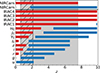 |
Fig. 1. Redshifts in which the different Euclid, IRAC, and ground-based filters trace the optical (red bars) or UV (blue bars) continuum. The grey shaded area indicates the redshift range in which we have at least four filters to derive the slopes necessary to select LRDs. The hatched area indicates the redshift range covered without IRAC. The first two bars, separated by a horizontal solid black line, indicate the redshift range in which at least two JWST NIRCam broad-band filters trace the rest-frame optical or UV continuum. |
The LRD redshifts are not correctly recovered by the standard Euclid pipeline (see Appendix B) because LRD templates are currently not included. We therefore included the redshift as a free parameter in the fit. We considered the median redshift from the pipeline as an initial guess and the first- and second- mode redshifts (i.e. first and second peak in the redshift probability distribution) as limits. For candidates at z > 6, the photometric redshift was derived considering a secondary branch of the pipeline. In this case, we therefore considered the first peak of the redshift probability distribution as the initial guess. The fit was performed with the Scipy package (Virtanen et al. 2020). To take possible unknown uncertainties into account, we added 5% of the flux in quadrature to the flux uncertainties. In the fit, we considered all available filters, but we included fluxes with S/N < 3 as 0 with an error equal to twice the flux uncertainties to take unknown uncertainties into account. The uncertainties on the output properties were derived by repeating the fit 100 times after randomising the fluxes, considering a Gaussian function centred on the measured value, and with σ equal to the flux uncertainties. The performance of the new redshift estimation and the redshift of the pipeline are analysed in Appendix B.
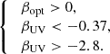
Following the selection made by Kocevski et al. (2025), we selected objects with
 (2)
(2)
The third cut to the UV slope was applied to remove contamination by brown dwarfs. These near-IR colours of these objects are similar to those of reddened AGNs, but they appear to be significantly bluer at shorter wavelengths (Langeroodi & Hjorth 2023). To ensure a v-shape SED when the two longest wavelength filters had S/N > 3, we also requested that the flux of the filter at the longest wavelength was the highest.
In order to select only compact sources, we considered sources with μmax − mpoint-like < −2.6 mag arcsec−2, which corresponds to the difference between the peak surface brightness (μmax) above the background in the detection band (IE for VIS-detected objects and JE + YE + HE for NISP-detected objects) and the expected magnitude for point-like sources (mpoint − like). The chosen threshold was optimised in the Euclid pipeline to select compact objects, such as stars (Euclid Collaboration: Romelli et al. 2026).
A red rest-frame optical continuum can be mimicked by strong nebular emission lines. We therefore performed an additional selection to remove such objects. In particular, the H α + [N II] complex is present in the YE filter at z = 0.44–0.85, in the JE filter at z = 0.77–1.39, in the HE filter at z = 1.31–2.09, and in the IRAC1 filter at z = 3.82–4.99. In these redshift intervals, we imposed that the flux of the contaminated band was lower than the flux of the next redward filter. A negative slope would indeed indicate strong nebular emission lines even when the overall optical slope is consistent with our LRD slope selection. Many previous JWST samples did not perform this selection, and the LRD optical colours may indeed be boosted by nebular emission lines (Hainline et al. 2025). A more complex analysis, which we leave for future studies, is necessary to understand whether the underlying continuum of these strong-line emitters is anyway consistent with the LRD selection, however.
We then studied the distribution of the χ2 and removed any object with χ2 ≥ 100. This threshold was chosen based on the overall distribution of χ2 and on a random selection of SED.
Finally, because the number of sources is limited, we visually verified the Euclid and IRAC cutouts of any remaining object to remove cases that were affected by blending issues in the IRAC bands, any remaining artefacts, or sources that were extended in the NISP filters. Future work that performs a detailed deblending analysis might improve over this step. This selection unfortunately removes potential close pairs, which some LRDs may be part of (e.g. Tanaka et al. 2024 found three dual LRD candidates over 0.54 deg2).
We also considered the photometric redshift estimation derived for NISP-detected sources that extend the redshift boundary at z > 6. As for the previous sample, we only selected reliable sources using the flagging available in the catalogue. We imposed a detection in the IRAC filters, an S/N > 3 in at least four bands, and only selected v-shaped and compact sources. The sources that we selected in the different steps are listed in Table 3, but we finally did not obtain any additional LRD candidates.
The search for LRDs at z = 1–2.1 can be performed without the IRAC filters because the JE and HE filters cover the rest-frame optical continuum (see Fig. 1). We therefore repeated the selections described above and limited the analysis to objects with a pipeline redshift zpipeline < 3 as a conservative cut, but removed any object that was detected in IRAC. As for the previous selection, we searched for objects that were detected in at least four filters (two blueward and two redward λbreak), with a v-shaped continuum, which were compact, had no evident contamination from strong nebular emission lines, and with χ2 < 100. We visually inspected the Euclid cutouts of any remaining object to remove any remaining artefact or extended objects.
The final sample of LRD candidates includes 29 objects with IRAC detections. This corresponds to a density of 0.8 deg−2. It also includes 3312 objects without IRAC detections and is limited to z ≤ 2.1, corresponding to a density of 57.3 deg−2. The total sample includes 3341 LRD candidates. The number of LRD candidates is conservative because of the uncertainties in the rest-frame UV and optical slopes we outlined in Appendix C and the conservative selection steps we performed. The complete list of LRD candidates and their properties is reported in Table D1, and the cutouts and photometric fit of two LRDs are shown as examples in Figs. 2 and 3. The Euclid point-spread function (PSF) is slightly undersampled in IE has a pixel scale of 0 1 and an FWHM = 0
 158–0
158–0 164 Euclid Collaboration: McCracken et al. (2026), which is reflected in the cutouts. The NISP images were instead interpolated to the same pixel scale as IE, but their pixel scale originally is 0
 3 and their FWHM = 0.35″.
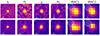 |
Fig. 2. Two example LRD candidates, showing cutouts of 4″ × 4″ in the four Euclid filters and the two shortest IRAC channels. From left to right: IE, YE, JE, HE, IRAC1, and IRAC2. We report the size of the PSF in the top left and the physical scale on the bottom left corner of each panel. |
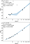 |
Fig. 3. Fit with two power-laws of the photometric data of the two example LRD candidates shown in Fig. 2. We show fluxes with S/N > 3 as black squares, and the 3σ upper limits are shown with empty triangles. The best fit is shown with a blue solid line, and the shaded region shows the 16% and 84% uncertainties. We report the χ2 and the output parameters in the top left corner. |
The redshift and magnitude distributions in the three fields are reported in Appendix E. They show that the selection is reasonably uniform across the fields.
3.2. Differences between the IRAC-detected and IRAC-undetected LRD candidates.
The difference in density of LRD candidates with and without IRAC is probably driven by several factors. On the one hand, the number of LRD candidates with IRAC may be underestimated because blending issues can affect IRAC fluxes. This produces a boost in the contaminated band that results in a large χ2, and we simultaneously performed a stricter visual check to remove any possible blended source. As shown in Table 3, the fraction of sources removed by the χ2 cut and the visual inspection is larger for IRAC-detected sources. To understand the importance of blending, we verified that about 15% of all reliable Euclid sources had a neighbour within 2″ (equal to the smallest IRAC FWHM) and that 5% of the sources had a neighbour within 1″. LRDs might cluster more strongly at kiloparsec scales (Tanaka et al. 2024), and the effect of blending might therefore be even stronger in LRDs than in the general galaxy population. In addition, the FWHM of IRAC is larger than the radius we used for the photometry, so that flux loss might effect the source detection.
On the other hand, the number of LRD candidates selected without IRAC may be overestimated because the H α + [N II] complex is contained within the HE filter at z = 1.31–2.09. The IRAC bands can help us to identify them. In addition, the wider wavelength coverage can simply improve the removal of any type of contaminants.
Some differences may be intrinsic, however. Observations with the JWST mid-infrared instrument (MIRI) have shown that the rest-frame continuum at λ ≳ 0.7 μm becomes remarkably flat. This indicates a mild contribution from an obscured AGN (Williams et al. 2024; Pérez-González et al. 2024) or an AGN torus without hot dust (Leung et al. 2024; Barro et al. 2024b). At z < 2.8, IRAC bands cover the same rest-frame wavelengths as MIRI at z > 5 (i.e. λ ≥ 0.7 μm). This covers the flatter part of the SED.
4. Results
4.1. Comparison with the JWST LRD catalogues
In Fig. 4 we show a comparison of the redshift and MUV at 1450 Å of our sample of LRD candidates, derived by fitting the available data with two power laws, as explained in detail in Appendix B. We also compare our results with some of the previous samples derived with JWST data (Kocevski et al. 2025; Labbé et al. 2023; Kokorev et al. 2024a). Our sample is complementary to the JWST samples that were derived so far because it covers brighter magnitudes. Only one JWST source is as bright as Euclid-selected sources. It is also clear that our sample extends to lower redshifts than the JWST sample. In the same figure, we also show the MUV that we expect to reach at the end of the Euclid mission. The EDFs will be two magnitudes deeper when completed. Even when the IRAC data remain unchanged, this will allow us to reach MUV = −20 at z = 4, which extends the overlap with JWST, but also probes the bright end up to z = 8.
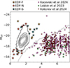 |
Fig. 4. MUV and redshift for all LRD candidates, shown as contour lines, equally spaced from 10% to 90%. The last line represents 99% of the distribution. The remaining 1% of the sample is shown with stars, colour-coded based on their field. We also show three samples of LRDs selected with JWST observations (Kocevski et al. 2025; Labbé et al. 2023; Kokorev et al. 2024a; Akins et al. 2024). The dotted black line shows the 80% completeness that is expected when the EDFs are at their final depth. |
It is necessary, however, to consider that even if we select only compact sources, the different angular resolution of JWST and Euclid might affect the selection. In Table 4 we report the FWHM of the two missions at similar wavelengths, with the corresponding physical scales given at z = 1 and z = 6. The difference with respect to IRAC is even larger and reaches a factor of at least 10 in physical size. Therefore, follow-up campaigns will be necessary to confirm that the LRD candidates identified with Euclid and IRAC are as compact as the JWST candidates.
FWHM of the Euclid VIS/NISP, JWST NIRCam, and IRAC PSFs.
To understand the level of contamination from the different angular resolutions of JWST and Euclid, we analysed the subsample of extended v-shape sources from Kocevski et al. (2025, priv. com.). These sources are mainly dusty star-forming galaxies and correspond to 14% of all v-shape sources, but their redshift distribution is skewed toward z < 4 (see Fig. 7 in Kocevski et al. 2025). In Fig. 5 we compare the size of these extended v-shape sources derived from the JWST/F444W filter with the angular resolution of Euclid. In particular, the JWST/F444W filter and the HE filter both trace the rest-frame optical of the LRDs up to z = 3.1 and can therefore be compared directly. This comparison clearly shows that the majority of these sources are also extended for Euclid. Only 8% (15) of them are below the HE filter FWHM at z = 2–4. Combining this finding with the redshift distribution of the LRD candidates by Kocevski et al. (2025), we obtained that we expect 15% of contaminants at z = 2–4.
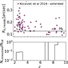 |
Fig. 5. Top: Half-light ratio in the JWST/F444W filter vs. redshift for the sample of extended v-shape objects by Kocevski et al. (2025). The horizontal solid line indicate the HE band FWHM, scaled assuming a Gaussian function. Bottom: Fraction of extended v-shape objects that is expected to be unresolved in the HE band as a function ofredshift. |
At lower redshift. these contaminants are expected to contribute even less, but we do not have direct measurements because the sample by Kocevski et al. (2025) is limited to z > 2. Considering the redshift evolution of the size mass relation for late-type galaxies (van der Wel et al. 2014), however, we expect a median increase in the galaxy size by 1.2 between z = 2.25 and z = 1.75 and 1.9 between z = 2.25 and z = 0.75. The smallest extended v-shape source at z < 4 by Kocevski et al. (2025) is only a factor of 0.88 of the Euclid angular resolution in the HE band. We therefore expect that all sources at z < 2 are resolved.
4.2. Comparison with other Euclid AGN catalogues
Other works have focused on the selection of AGNs and mainly used Q1 photometric data. We therefore investigated the amount of overlap with our sample of LRD candidates. In particular, the Euclid AGN catalogue presented by Euclid Collaboration: Matamoro Zatarain et al. (2026) focused on the selection of AGN, mainly blue QSOs, based on Euclid photometry, but also on ancillary data from UV to IR, and previous public spectroscopic data. Euclid Collaboration: Roster et al. (2026) instead matched Euclid sources with public X-ray surveys and identified X-ray detected AGNs. The details of these selections and the overlap with our samples of LRD candidates is reported in Appendix F. No sources are identified by all QSO selections in de EDF-F and EDF-S overall, and 1898 (80%) are selected by at least one criterion. In the EDF-N, 816 sources, which corresponds to 84% of the EDF-N sample of LRD candidates, is selected by at least one QSO criterion, while no sources are selected by all criteria.
4.3. LRDs luminosity function
To measure the UV luminosity function of our sample of LRD candidates, we used the 1/Vmax method (Rowan-Robinson 1968; Schmidt 1968). In particular, the luminosity for each magnitude and redshift bin is defined as
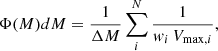 (3)
(3)
where ΔM is the width of the magnitude bin, wi is the completeness correction for the ith object, and Vmax,i is the maximum comoving volume at which object i could have been detected. To calculate the latter, we considered the area that is covered by the observations, the minimum redshift of the bin, and the maximum redshift at which each source could be observed. The latter was derived considering the v-shaped model of each source, described by two power laws with slopes βUV, i and βopt, i, normalised to the absolute UV magnitude (MUV, i). This model was then shifted from the minimum to the maximum redshift of the redshift bin and was convolved at each redshift step with the Euclid and ancillary bands to estimate the expected fluxes. These fluxes were then used to derive the maximum redshift at which we would have at least four filters with S/N > 3.
4.3.1. Area
The area associated with each field was derived considering the coverage map for the four Euclid filters, combined to remove the area in which at least one filter was masked. In addition, we also removed additional masked areas that covered bright stars, both halo and ground-bleeding trails, and extended bright foreground sources. In addition, we combined these masks with the coverage by IRAC to derive the area associated with IRAC-detected sources. The areas we considered are listed in Table 5.
Area in deg2 used to estimate the LRD luminosity function.
4.3.2. Completeness limits and correction
To derive the 80% completeness limit of our sample, we derived the fraction of LRDs with at least four filters with S/N > 3 as a function of redshift and MUV. In particular, we considered redshift bins of Δz = 0.25 up to z = 6, since no LRDs are found at higher redshifts. We also considered magnitude bins of ΔMUV = 0.25 from MUV = −25 to MUV = −10. In each redshift-magnitude bin, we randomly extracted 1000 βUV and βopt values from the observed distribution. We then derived the fraction of these mock LRDs that were observed in at least four filters with S/N > 3, considering the depths of the different fields reported in Table 1. We used this estimate to correct the derived luminosity function.
We also applied the corrections for incorrect redshifts that we derived from the analysis of the redshift recovery on the simulated sample in Appendix B. This correction varied from 0.6 for z = 1–1.5 because the number of sources in this redshift range is expected to be overestimated, to 1.3 for z = 2–2.5, where the number of objects is underestimated instead. A more detailed completeness correction that takes the compactness of the sources into account, for example, will be estimated in future works when the systematic effects of the telescope are understood better.
Finally, we considered a correction of 15% due to the contamination by extended sources that are unresolved by Euclid (see Sect. 4.1). This contamination is expected to increase at z > 6, but we found no LRD candidates at these high-z values. At the same time, this correction is expected to decrease at z < 2 due to the average increase of galaxy size with decreasing redshift, but we lack the data to properly quantify this decrease. As a conservative approach, we therefore applied the same correction at all redshifts.
4.3.3. Uncertainties
We estimated the uncertainties of the luminosity function by performing a bootstrap analysis of the sample. We generated 100 random samples starting from the entire LRD sample. In every realisation, we also randomised the redshift and the absolute UV magnitude considering a Gaussian function centred on the best-fit value and with a standard deviation equal to their respective uncertainties. We added the Poisson errors in quadrature to these uncertainties, following the prescription by Gehrels (1986). We did not include any uncertainty due to cosmic variance because the areas we analysed are so large.
4.3.4. Estimated luminosity functions
We derived the UV luminosity functions of LRDs as explained in the previous sections and considering the following redshift bins: 0.6 ≤ z < 1.0; 1.0 ≤ z < 1.5; 1.5 ≤ z < 2.0; 2.0 ≤ z < 2.5; and 2.5 ≤ z < 4.0. In the first redshift bin, we only considered objects in EDF-N because the other fields lack the u-band observations necessary to properly trace the UV slope. Eleven objects (0.3% of the sample) were not considered in the UV luminosity functions because they correspond to a redshift at which the UV slope is not properly covered. The derived UV luminosity functions are shown in Fig. 6, where we also compare our results with UV luminosity functions from the literature of LRDs based on JWST data (Kokorev et al. 2024a; Kocevski et al. 2025) and QSOs, including JWST data (Maiolino et al. 2024b; Harikane et al. 2023; Grazian et al. 2024) or before JWST (Giallongo et al. 2012, 2015; McGreer et al. 2013; Akiyama et al. 2018; Niida et al. 2020; Pan et al. 2022). The values of the LRD luminosity function of this work are also reported in Table 6. When these results are analysed, it is necessary to consider that the luminosity function based on Euclid data alone may be overestimated because some contaminants might not have been properly included in the corrections. On the other hand, the luminosity function based on IRAC observations might be severely underestimated because we strictly removed any source that was affected by blending.
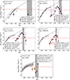 |
Fig. 6. UV luminosity function of the LRD candidates from z = 0 (top left) to z = 4 (bottom right). The empty stars indicate the values before any corrections, and the coloured stars show the density after correcting for completeness and redshift estimation. The coloured triangles show the conservative estimation derived considering only IRAC-detected sources. The vertical shaded black regions show the range of the 80% completeness in the three fields. In the top left corner, we report the number of objects inside the redshift bin, and we show the number of IRAC-detected sources in the bin in brackets. The empty symbols show UV luminosity functions of QSOs from Giallongo et al. (2012, and reference therein), Akiyama et al. (2018), and Pan et al. (2022). We also report the UV luminosity function of QSOs modelled by Kulkarni et al. (2019, dashed black line). For a comparison, the horizontal dash-dotted red line shows the minimum density probed by the HST CANDELS survey (0.29 deg2Grogin et al. 2011; Koekemoer et al. 2011), and the horizontal dotted red line shows the minimum density probed by the JWST COSMOS-WEB survey (0.54 deg2 Casey et al. 2023). |
UV luminosity function of LRD candidates.
In the highest-redshift bin (i.e. 4.0 ≤ z < 6.0), we found no candidates. This prevents comparisons with previous JWST results. We must therefore wait for future Euclid releases to improve over these results. The depth of the EDFs is expected to increase by two magnitudes until the end of the mission (Euclid Collaboration: Mellier et al. 2025). We predict that with the final depths of the EDFs, Euclid will be able to observe the brightest LRDs observed by JWST so far (Fig. 4).
At redshifts z < 4, we can only compare our results to previous QSO UV luminosity functions because observations of LRDs with JWST were mainly limited to z > 4. The luminosity function of the LRDs is always well below the QSO luminosity functions at bright magnitudes by 1.2–2.6 dex, which corresponds to 1–4σ because of the low number statistics, however. This difference generally indicates that LRDs are not the dominant AGN population at these magnitudes at z < 4, assuming they are AGNs. The LRD luminosity functions are instead closer to the QSO luminosity functions at at z > 1 and at the faintest magnitudes probed by this work. The closest point is at 1.5 ≤ z < 2.0, where the LRD luminosity function is only 0.7 dex below the QSO luminosity function about MUV = −19.25 mag, but given the large statistics, the uncertainties are small, and this difference corresponds to more than 10σ. We cannot verify whether the LRD luminosity function is closer to the QSO luminosity function at even fainter magnitudes because ofincompleteness.
In the same figure, we also report the maximum volume probed by one of the largest JWST survey so far, that is, COSMOS-Web (Casey et al. 2023), which covers 0.6 deg2 (dotted red line in Fig. 6), and the Cosmic Assembly Near-infrared Deep Extragalactic Legacy Survey (CANDELS Grogin et al. 2011; Koekemoer et al. 2011), which covers 0.29 deg2 with the Hubble Space Telescope (HST; dash-dotted red line in Fig. 6). At z < 1 and z > 2.5, the area of these two surveys is too small to observe a significant number of objects with luminosities similar to the candidates we selected. We would expect to observe some objects at the other redshifts, however:  at 1.0 ≤ z < 1.5;
  at 1.5 ≤ z < 2.0; and
  at 2.0 ≤ z < 2.5 in CANDELS;
  at 1.0 ≤ z < 1.5;
  at 1.5 ≤ z < 2.0; and
  at 2.0 ≤ z < 2.5 in COSMOS-Web. At these redshifts, however, no LRD was identified with HST and only a few were identified with JWST. For example, Kocevski et al. (2025) found 17 LRD candidates at z < 4. Based on the LRD luminosity function we found here, we would expect
  candidates in this area. This difference (2σ deviation) in number density may be due to contaminants or to the different angular resolution of Euclid and JWST. This means that future follow-up studies are fundamental. It is important to note, however, that the number density of the subsample of more robust LRD candidates, which are those that are also observed by IRAC, is too low to be detected by any JWST or HST survey.
We also report the conservative luminosity function derived with the IRAC-detected sources alone, which have more constraints, but were also cleaned more severly to avoid blending issues. This estimates are compatible with the few LRD candidates at z < 4 that were observed by JWST and HST.
A comparison between the LRDs UV luminosity functions we derived is shown in Fig. 7. This plot shows a tentative evolution of the luminosity function with redshift. The density of LRD candidates increases from the high redshift to z = 1.5–2.5 and decreases at even lower redshifts. For example, at 1.5 ≤ z < 2.0 and MUV = −20.25 mag, we obtained a density of  . Our estimate at the same magnitude but at 2.0 ≤ z < 2.5 is slightly lower, that is
  , but it may be incomplete given the necessity of using IRAC data at z > 2.1. In contrast, the drop at z < 1.5 is not linked to observational biases because we expect Euclid data to have the same capacity of selecting LRDs down to z = 0.7. To give a more quantitative estimate, at MUV = −19.25 mag, the LRD density is
  at 1.0 ≤ z < 1.5 and it is
  at 1.5 ≤ z < 2.0, with a drop of 0.67 dex. The statistics in the lowest-redshift bin are quite poor because it is based on the EDF-N alone. This prevents us from further exploring the possible redshift evolution. The density of LRD candidates with MUV ≥ −21 mag at 1 ≤ z < 2.5 is also similar to the density derived with JWST at 4 ≤ z < 6 (Kocevski et al. 2025; Kokorev et al. 2024a), however, which is log10(N Mpc−3 mag−1) =−5.19 ± 0.20 and log10(N Mpc−3 mag−1) =−5.10 ± 0.1 respectively. This supports the idea that the high-z evolution might be due to incompleteness in our LRD sample. This evolution is absent when we only consider the few LRD candidates that were detected in IRAC because the statistics is too low.
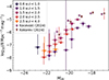 |
Fig. 7. Comparison of the corrected UV luminosity function of LRD candidates from z = 0 to z = 4, and values at z = 6 from the literature (Kocevski et al. 2025; Kokorev et al. 2024a). |
Overall, we speculate that the LRD number density seems to remain constant from z = 4–6 to z = 1.5–2.5, and this resembles the observed evolution of the star formation rate density (e.g. Madau & Dickinson 2014; Gruppioni et al. 2020; Traina et al. 2024), the BH accretion rate density (e.g. Delvecchio et al. 2014), and the evolution in the molecular gas mass (see Tacconi et al. 2020, for a review). When we consider that LRDs may be very dense and dust-obscured starbursts or obscured SMBHs that might accrete at a super-Eddingthon rate, their frequency might follow the trend for the more general population of star-forming galaxies or AGNs, which is at the end regulated by the availability of cold gas.
Further analysis is needed to understand the level of contamination in our sample or why these LRD candidates have been missed by previous JWST studies. These sources might also not be as compact as those that are observed with JWST, which are compact when the spatial resolution of Euclid is considered, but not with JWST, which is 4–6 times better that the Euclid’s. Following the estimates from Sect. 4.1 we considered 15% of such contaminants in estimating the luminosity function, but detailed spectroscopic follow-ups are necessary to properly quantify the purity of our sample of LRD candidates. If the sample is dominated by contaminants, considering that the number densities seems to remain similar from z = 6 to z = 2, we might be following different evolutionary stages of the same galaxypopulation.
As the depth of the EDFs increases and the spectroscopic coverage improves, the identification of LRDs and the estimation of their properties will improve in the future. This will enable us to derive more conclusive results on the possible redshift evolution of the LRD luminosity function.
5. Conclusions
We have taken advantage of the Euclid Q1 data that cover about 63 deg2 to search for LRD candidates. The selection was performed by exploiting Euclid photometric data, ground-based ancillary data, and Spitzer/IRAC data. After a conservative selection that included conservative flagging and a visual inspection of all candidates, we obtained a final sample of 3341 LRD candidates, 29 of which are also detected with IRAC.
Even when we imposed a S/N > 3 in at least four filters, LRD candidates are relatively faint, with means magnitudes of IE = 25.5, YE = 24.3, JE = 24.0, and HE = 23.7. These are fainter than the 5σ limits of the Q1 data release. Their photometric redshift was estimated to range between z = 0.33 and z = 3.6, where previous JWST selections identified a rapid decline in the number of LRD candidates. At z > 4, the depth of the ancillary IRAC data limits our sample to only the brightest sources, however.
We also derived the rest-frame UV luminosity function, but found no overlap in the parameter space of Euclid and JWST. This limited the direct comparison. Euclid is complementary to JWST observations because it can probe the bright end of the UV luminosity function because the covered area is so large. The most puzzling result is that the UV luminosity function of LRD candidates increases from high z to z = 1.5–2.5, below which it decreases again. This is in contrast with previous JWST results, which derived a drastic drop in LRDs at z < 4, with almost no candidates at z < 2. The z > 4 evolution of our luminosity function may be affected by incompleteness in our LRD candidate sample, however. It is important to note that no significant evolution is apparent in the subsample of more robust LRD candidates that are also detected by IRAC, which has poor statistics (only 29 objects), however, and is limited by the IRAC resolution. Clearly, more observations are required to clarify this situation. Another interesting result is that the LRD UV luminosity function remains below the QSO luminosity function, except at MUV > −21, where they become compatible. This might indicate that if LRDs are indeed AGNs, they are a sub-dominant AGN population.
Further analyses are necessary to validate the LRD candidates of this work and optimise the removal of possible contaminants. In addition, further critical studies need to probe their structure and determine their compatibility with JWST sources because of the different spatial resolution of the two telescopes. If a sizeable fraction of the LRD candidates we identified are confirmed by future studies, it will enable us to study the redshift evolution over a broad redshift and luminosity range. This will help us to shed light on these mysterious sources. Future Euclid data releases are expected to increase the number of LRD candidates, but also to increase the overlap in parameter space with previous JWST samples, as the Euclid Wide survey will be wider than the Q1 at similar depth, while the Euclid Deep survey will be considerably deeper. In addition, a direct comparison between JWST and Euclid selections will be possible in future releases because Euclid will cover some of the area that was already observed with JWST.
Data availability
Full table D1 is available at the CDS via https://cdsarc.cds.unistra.fr/viz-bin/cat/J/A+A/711/A24
Acknowledgments
The research activities described in this paper were carried out with contribution of the Next Generation EU funds within the National Recovery and Resilience Plan (PNRR), Mission 4 – Education and Research, Component 2 – From Research to Business (M4C2), Investment Line 3.1 – Strengthening and creation of Research Infrastructures, Project IR0000034–“STILES – Strengthening the Italian Leadership in ELT and SKA”. This work has benefited from the support of Royal Society Research Grant RGS\R1\231450. This research was supported by the International Space Science Institute (ISSI) in Bern, through ISSI International Team project #23-573 “Active Galactic Nuclei in Next Generation Surveys”. L.B., F.R., and V.A acknowledge the support from the INAF Large Grant “AGN & Euclid: a close entanglement” Ob. Fu. 01.05.23.01.14. A.F. acknowledges the support from project “VLT- MOONS” CRAM 1.05.03.07, INAF Large Grant 2022 “The metal circle: a new sharp view of the baryon cycle up to Cosmic Dawn with the latest generation IFU facilities” and INAF Large Grant 2022 “Dual and binary SMBH in the multi-messenger era”. L.B. thanks A. Marasco for computational support and D. Kocevski for providing the data necessary for comparing the Euclid LRD candidates with the JWST ones. This research made use of Photutils, an Astropy package for detection and photometry of astronomical sources (Bradley et al. 2023). The Euclid Consortium acknowledges the European Space Agency and a number of agencies and institutes that have supported the development of Euclid, in particular the Agenzia Spaziale Italiana, the Austrian Forschungsförderungsgesellschaft funded through BMIMI, the Belgian Science Policy, the Canadian Euclid Consortium, the Deutsches Zentrum für Luft- und Raumfahrt, the DTU Space and the Niels Bohr Institute in Denmark, the French Centre National d’Etudes Spatiales, the Fundação para a Ciência e a Tecnologia, the Hungarian Academy of Sciences, the Ministerio de Ciencia, Innovación y Universidades, the National Aeronautics and Space Administration, the National Astronomical Observatory of Japan, the Netherlandse Onderzoekschool Voor Astronomie, the Norwegian Space Agency, the Research Council of Finland, the Romanian Space Agency, the State Secretariat for Education, Research, and Innovation (SERI) at the Swiss Space Office (SSO), and the United Kingdom Space Agency. A complete and detailed list is available on the Euclid web site (www.euclid-ec.org). This work has made use of the Euclid Quick Release Q1 data from the Euclid mission of the European Space Agency (ESA), 2025, https://doi.org/10.57780/esa-2853f3b. Based on data from UNIONS, a scientific collaboration using three Hawaii-based telescopes: CFHT, Pan-STARRS, Subaru www.skysurvey.cc. Based on data from the Dark Energy Camera (DECam) on the Blanco 4-m Telescope at CTIO in Chile https://www.darkenergysurvey.org. This work uses results from the ESA mission Gaia, whose data are being processed by the Gaia Data Processing and Analysis Consortium https://www.cosmos.esa.int/gaia. This publication is based on observations made with the Spitzer Space Telescope, which is operated by the Jet Propulsion Laboratory, California Institute of Technology under a contract with NASA, and has made use of the NASA/IPAC Infrared Science Archive, which is funded by the National Aeronautics and Space Administration and operated by the California Institute ofTechnology.
References
- Abbott, T. M. C., Abdalla, F. B., Allam, S., et al. 2018, ApJS, 239, 18 [Google Scholar]
- Akins, H. B., Casey, C. M., Lambrides, E., et al. 2024, ApJ, submitted [arXiv:2406.10341] [Google Scholar]
- Akiyama, M., He, W., Ikeda, H., et al. 2018, PASJ, 70, S34 [NASA ADS] [CrossRef] [Google Scholar]
- Alexander, T., & Natarajan, P. 2014, Science, 345, 1330 [NASA ADS] [CrossRef] [Google Scholar]
- Ananna, T. T., Bogdán, Á., Kovács, O. E., Natarajan, P., & Hickox, R. C. 2024, ApJ, 969, L18 [NASA ADS] [CrossRef] [Google Scholar]
- Assef, R. J., Stern, D., Noirot, G., et al. 2018, ApJS, 234, 23 [Google Scholar]
- Asthana, S., Haehnelt, M. G., Kulkarni, G., et al. 2024, arXiv e-prints [arXiv:2409.15453] [Google Scholar]
- Atek, H., Labbé, I., Furtak, L. J., et al. 2024, Nature, 626, 975 [NASA ADS] [CrossRef] [Google Scholar]
- Baggen, J. F. W., van Dokkum, P., Brammer, G., et al. 2024, ApJ, 977, L13 [NASA ADS] [CrossRef] [Google Scholar]
- Barkana, R., & Loeb, A. 2001, Phys. Rep., 349, 125 [NASA ADS] [CrossRef] [Google Scholar]
- Barro, G., Perez-Gonzalez, P. G., Kocevski, D. D., et al. 2024a, ApJ, 963, 128 [CrossRef] [Google Scholar]
- Barro, G., Perez-Gonzalez, P. G., Kocevski, D. D., et al. 2024b, arXiv e-prints [arXiv:2412.01887] [Google Scholar]
- Begelman, M. C., & Volonteri, M. 2017, MNRAS, 464, 1102 [NASA ADS] [CrossRef] [Google Scholar]
- Bellovary, J. 2025, ApJ, 984, L55 [Google Scholar]
- Bisigello, L., Giulietti, M., Prandoni, I., et al. 2025, Open J. Astrophys., 8, 101 [Google Scholar]
- Bradley, L., Sipőcz, B., Robitaille, T., et al. 2023, https://doi.org/10.5281/zenodo.1035865 [Google Scholar]
- Carr, B. J., & Hawking, S. W. 1974, MNRAS, 168, 399 [NASA ADS] [CrossRef] [Google Scholar]
- Casey, C. M., Kartaltepe, J. S., Drakos, N. E., et al. 2023, ApJ, 954, 31 [NASA ADS] [CrossRef] [Google Scholar]
- Dayal, P. 2024, A&A, 690, A182 [NASA ADS] [CrossRef] [EDP Sciences] [Google Scholar]
- Dayal, P., & Ferrara, A. 2018, Phys. Rep., 780, 1 [Google Scholar]
- Dayal, P., Volonteri, M., Greene, J. E., et al. 2025, A&A, 697, A211 [NASA ADS] [CrossRef] [EDP Sciences] [Google Scholar]
- Decleir, M., Gordon, K. D., Andrews, J. E., et al. 2022, ApJ, 930, 15 [NASA ADS] [CrossRef] [Google Scholar]
- Delvecchio, I., Gruppioni, C., Pozzi, F., et al. 2014, MNRAS, 439, 2736 [NASA ADS] [CrossRef] [Google Scholar]
- Delvecchio, I., Daddi, E., Sargent, M. T., et al. 2022, A&A, 668, A81 [NASA ADS] [CrossRef] [EDP Sciences] [Google Scholar]
- DESI Collaboration (Adame, A. G., et al.) 2024, AJ, 168, 58 [NASA ADS] [CrossRef] [Google Scholar]
- Donley, J. L., Koekemoer, A. M., Brusa, M., et al. 2012, ApJ, 748, 142 [Google Scholar]
- Euclid Collaboration (Moneti, A., et al.) 2022, A&A, 658, A126 [NASA ADS] [CrossRef] [EDP Sciences] [Google Scholar]
- Euclid Collaboration (Bisigello, L., et al.) 2024, A&A, 691, A1 [NASA ADS] [CrossRef] [EDP Sciences] [Google Scholar]
- Euclid Collaboration (Cropper, M., et al.) 2025, A&A, 697, A2 [Google Scholar]
- Euclid Collaboration (Jahnke, K., et al.) 2025, A&A, 697, A3 [Google Scholar]
- Euclid Collaboration (McPartland, C. J. R., et al.) 2025, A&A, 695, A259 [Google Scholar]
- Euclid Collaboration (Mellier, Y., et al.) 2025, A&A, 697, A1 [Google Scholar]
- Euclid Collaboration (Zalesky, L., et al.) 2025, A&A, 695, A229 [Google Scholar]
- Euclid Collaboration (Aussel, H., et al.) 2026, A&A, 711, A1 (Euclid Q1 SI) [Google Scholar]
- Euclid Collaboration (Margalef-Bentabol, B., et al.) 2026, A&A, 711, A18 (Euclid Q1 SI) [Google Scholar]
- Euclid Collaboration (Matamoro Zatarain, T., et al.) 2026, A&A, 711, A20 (Euclid Q1 SI) [Google Scholar]
- Euclid Collaboration (McCracken, H. J., et al.) 2026, A&A, 711, A2 (Euclid Q1 SI) [Google Scholar]
- Euclid Collaboration (Polenta, G., et al.) 2026, A&A, 711, A3 (Euclid Q1 SI) [Google Scholar]
- Euclid Collaboration (Romelli, E., et al.) 2026, A&A, 711, A4 (Euclid Q1 SI) [Google Scholar]
- Euclid Collaboration (Roster, W., et al.) 2026, A&A, 711, A16 (Euclid Q1 SI) [Google Scholar]
- Euclid Collaboration (Tucci, M., et al.) 2026, A&A, 711, A5 (Euclid Q1 SI) [Google Scholar]
- Euclid Quick Release Q1 2025, https://doi.org/10.57780/esa-2853f3b [Google Scholar]
- Ferrarese, L. 2002, ApJ, 578, 90 [NASA ADS] [CrossRef] [Google Scholar]
- Fitzpatrick, E. L., Massa, D., Gordon, K. D., Bohlin, R., & Clayton, G. C. 2019, ApJ, 886, 108 [Google Scholar]
- Fumagalli, M., Patel, S. G., Franx, M., et al. 2012, ApJ, 757, L22 [NASA ADS] [CrossRef] [Google Scholar]
- Furtak, L. J., Zitrin, A., Plat, A., et al. 2023, ApJ, 952, 142 [NASA ADS] [CrossRef] [Google Scholar]
- Gaia Collaboration (Vallenari, A., et al.) 2023, A&A, 674, A1 [NASA ADS] [CrossRef] [EDP Sciences] [Google Scholar]
- Gebhardt, K., Bender, R., Bower, G., et al. 2000, ApJ, 539, L13 [Google Scholar]
- Gehrels, N. 1986, ApJ, 303, 336 [Google Scholar]
- Giallongo, E., Menci, N., Fiore, F., et al. 2012, ApJ, 755, 124 [NASA ADS] [CrossRef] [Google Scholar]
- Giallongo, E., Grazian, A., Fiore, F., et al. 2015, A&A, 578, A83 [NASA ADS] [CrossRef] [EDP Sciences] [Google Scholar]
- Glikman, E., Urrutia, T., Lacy, M., et al. 2012, ApJ, 757, 51 [Google Scholar]
- Glikman, E., Simmons, B., Mailly, M., et al. 2015, ApJ, 806, 218 [Google Scholar]
- Gordon, K. D., Cartledge, S., & Clayton, G. C. 2009, ApJ, 705, 1320 [NASA ADS] [CrossRef] [Google Scholar]
- Gordon, K. D., Misselt, K. A., Bouwman, J., et al. 2021, ApJ, 916, 33 [NASA ADS] [CrossRef] [Google Scholar]
- Gordon, K. D., Clayton, G. C., Decleir, M., et al. 2023, ApJ, 950, 86 [CrossRef] [Google Scholar]
- Grazian, A., Giallongo, E., Boutsia, K., et al. 2024, ApJ, 974, 84 [Google Scholar]
- Greene, J. E., Labbe, I., Goulding, A. D., et al. 2024, ApJ, 964, 39 [CrossRef] [Google Scholar]
- Grogin, N. A., Kocevski, D. D., Faber, S. M., et al. 2011, ApJS, 197, 35 [NASA ADS] [CrossRef] [Google Scholar]
- Gruppioni, C., Béthermin, M., Loiacono, F., et al. 2020, A&A, 643, A8 [NASA ADS] [CrossRef] [EDP Sciences] [Google Scholar]
- Gültekin, K., Richstone, D. O., Gebhardt, K., et al. 2009, ApJ, 698, 198 [Google Scholar]
- Habouzit, M., Pisani, A., Goulding, A., et al. 2020, MNRAS, 493, 899 [NASA ADS] [CrossRef] [Google Scholar]
- Habouzit, M., Li, Y., Somerville, R. S., et al. 2021, MNRAS, 503, 1940 [NASA ADS] [CrossRef] [Google Scholar]
- Hainline, K. N., Maiolino, R., Juodzbalis, I., et al. 2025, ApJ, 979, 138 [Google Scholar]
- Harikane, Y., Zhang, Y., Nakajima, K., et al. 2023, ApJ, 959, 39 [NASA ADS] [CrossRef] [Google Scholar]
- Hawking, S. 1971, MNRAS, 152, 75 [Google Scholar]
- Hickox, R. C., & Alexander, D. M. 2018, ARA&A, 56, 625 [Google Scholar]
- Inayoshi, K., & Maiolino, R. 2025, ApJ, 980, L27 [Google Scholar]
- Inayoshi, K., Haiman, Z., & Ostriker, J. P. 2016, MNRAS, 459, 3738 [NASA ADS] [CrossRef] [Google Scholar]
- Juodžbalis, I., Ji, X., Maiolino, R., et al. 2024, MNRAS, 535, 853 [CrossRef] [Google Scholar]
- Killi, M., Watson, D., Brammer, G., et al. 2024, A&A, 691, A52 [NASA ADS] [CrossRef] [EDP Sciences] [Google Scholar]
- Kocevski, D. D., Onoue, M., Inayoshi, K., et al. 2023, ApJ, 954, L4 [NASA ADS] [CrossRef] [Google Scholar]
- Kocevski, D. D., Finkelstein, S. L., Barro, G., et al. 2025, ApJ, 986, 126 [Google Scholar]
- Koekemoer, A. M., Faber, S. M., Ferguson, H. C., et al. 2011, ApJS, 197, 36 [NASA ADS] [CrossRef] [Google Scholar]
- Kokorev, V., Caputi, K. I., Greene, J. E., et al. 2024a, ApJ, 968, 38 [NASA ADS] [CrossRef] [Google Scholar]
- Kokorev, V., Chisholm, J., Endsley, R., et al. 2024b, ApJ, 975, 178 [Google Scholar]
- Kokubo, M., & Harikane, Y. 2024, ApJ, submitted [arXiv:2407.04777] [Google Scholar]
- Kulkarni, G., Worseck, G., & Hennawi, J. F. 2019, MNRAS, 488, 1035 [Google Scholar]
- Labbé, I., van Dokkum, P., Nelson, E., et al. 2023, Nature, 616, 266 [CrossRef] [Google Scholar]
- Labbe, I., Greene, J. E., Bezanson, R., et al. 2025, ApJ, 978, 92 [NASA ADS] [CrossRef] [Google Scholar]
- Langeroodi, D., & Hjorth, J. 2023, ApJ, 957, L27 [NASA ADS] [CrossRef] [Google Scholar]
- Leung, G. C. K., Finkelstein, S. L., Pérez-González, P. G., et al. 2024, ApJ, submitted [arXiv:2411.12005] [Google Scholar]
- Lin, R., Zheng, Z.-Y., Jiang, C., et al. 2025, ApJ, 980, L34 [Google Scholar]
- Madau, P., & Dickinson, M. 2014, ARA&A, 52, 415 [Google Scholar]
- Madau, P., Giallongo, E., Grazian, A., & Haardt, F. 2024, ApJ, 971, 75 [NASA ADS] [CrossRef] [Google Scholar]
- Magorrian, J., Tremaine, S., Richstone, D., et al. 1998, ApJ, 115, 2285 [CrossRef] [Google Scholar]
- Maiolino, R., Scholtz, J., Witstok, J., et al. 2024a, Nature, 627, 59 [NASA ADS] [CrossRef] [Google Scholar]
- Maiolino, R., Scholtz, J., Curtis-Lake, E., et al. 2024b, A&A, 691, A145 [NASA ADS] [CrossRef] [EDP Sciences] [Google Scholar]
- Maiolino, R., Risaliti, G., Signorini, M., et al. 2025, MNRAS, 538, 1921 [Google Scholar]
- Matthee, J., Naidu, R. P., Brammer, G., et al. 2024, ApJ, 963, 129 [NASA ADS] [CrossRef] [Google Scholar]
- Mazzolari, G., Gilli, R., Maiolino, R., et al. 2026, A&A, 706, A372 [NASA ADS] [CrossRef] [EDP Sciences] [Google Scholar]
- McGreer, I. D., Jiang, L., Fan, X., et al. 2013, ApJ, 768, 105 [NASA ADS] [CrossRef] [Google Scholar]
- Mezcua, M., Pacucci, F., Suh, H., Siudek, M., & Natarajan, P. 2024, ApJ, 966, L30 [NASA ADS] [CrossRef] [Google Scholar]
- Mullaney, J. R., Daddi, E., Béthermin, M., et al. 2012, ApJ, 753, L30 [Google Scholar]
- Netzer, H. 2015, ARA&A, 53, 365 [Google Scholar]
- Niida, M., Nagao, T., Ikeda, H., et al. 2020, ApJ, 904, 89 [NASA ADS] [CrossRef] [Google Scholar]
- Noboriguchi, A., Inoue, A. K., Nagao, T., Toba, Y., & Misawa, T. 2023, ApJ, 959, L14 [Google Scholar]
- Oke, J. B., & Gunn, J. E. 1983, ApJ, 266, 713 [NASA ADS] [CrossRef] [Google Scholar]
- Pacucci, F., & Loeb, A. 2022, MNRAS, 509, 1885 [Google Scholar]
- Pacucci, F., Natarajan, P., Volonteri, M., Cappelluti, N., & Urry, C. M. 2017, ApJ, 850, L42 [NASA ADS] [CrossRef] [Google Scholar]
- Pan, Z., Jiang, L., Fan, X., Wu, J., & Yang, J. 2022, ApJ, 928, 172 [NASA ADS] [CrossRef] [Google Scholar]
- Pérez-González, P. G., Barro, G., Rieke, G. H., et al. 2024, ApJ, 968, 4 [CrossRef] [Google Scholar]
- Reis, I., Baron, D., & Shahaf, S. 2019, AJ, 157, 16 [Google Scholar]
- Richards, G. T., Hall, P. B., Vanden Berk, D. E., et al. 2003, AJ, 126, 1131 [Google Scholar]
- Rigby, J., Perrin, M., McElwain, M., et al. 2023, PASP, 135, 048001 [NASA ADS] [CrossRef] [Google Scholar]
- Rowan-Robinson, M. 1968, MNRAS, 138, 445 [Google Scholar]
- Salvato, M., Wolf, J., Dwelly, T., et al. 2022, A&A, 661, A3 [NASA ADS] [CrossRef] [EDP Sciences] [Google Scholar]
- Schmidt, M. 1968, ApJ, 151, 393 [Google Scholar]
- Silk, J., & Rees, M. J. 1998, A&A, 331, L1 [NASA ADS] [Google Scholar]
- Simmonds, C., Tacchella, S., Hainline, K., et al. 2024, MNRAS, 535, 2998 [NASA ADS] [CrossRef] [Google Scholar]
- Stepney, M., Banerji, M., Tang, S., et al. 2024, MNRAS, 533, 2948 [CrossRef] [Google Scholar]
- Tacconi, L. J., Genzel, R., & Sternberg, A. 2020, ARA&A, 58, 157 [NASA ADS] [CrossRef] [Google Scholar]
- Tanaka, T. S., Silverman, J. D., Shimasaku, K., et al. 2024, arXiv e-prints [arXiv:2412.14246] [Google Scholar]
- Tee, W. L., Fan, X., Wang, F., & Yang, J. 2025, ApJ, 983, L26 [Google Scholar]
- Traina, A., Gruppioni, C., Delvecchio, I., et al. 2024, A&A, 681, A118 [NASA ADS] [CrossRef] [EDP Sciences] [Google Scholar]
- Urrutia, T., Lacy, M., & Becker, R. H. 2008, ApJ, 674, 80 [Google Scholar]
- van der Wel, A., Franx, M., van Dokkum, P. G., et al. 2014, ApJ, 788, 28 [Google Scholar]
- Virtanen, P., Gommers, R., Oliphant, T. E., et al. 2020, Nat. Methods, 17, 261 [Google Scholar]
- Wang, B., Leja, J., de Graaff, A., et al. 2024, ApJ, 969, L13 [NASA ADS] [CrossRef] [Google Scholar]
- Webster, R. L., Francis, P. J., Petersont, B. A., Drinkwater, M. J., & Masci, F. J. 1995, Nature, 375, 469 [Google Scholar]
- Wethers, C. F., Banerji, M., Hewett, P. C., et al. 2018, MNRAS, 475, 3682 [Google Scholar]
- Williams, C. C., Alberts, S., Ji, Z., et al. 2024, ApJ, 968, 34 [NASA ADS] [CrossRef] [Google Scholar]
- Wyithe, J. S. B., & Loeb, A. 2012, MNRAS, 425, 2892 [NASA ADS] [CrossRef] [Google Scholar]
- Yue, M., Eilers, A.-C., Ananna, T. T., et al. 2024, ApJ, 974, L26 [CrossRef] [Google Scholar]
- Zhang, Z., Jiang, L., Liu, W., & Ho, L. C. 2025, ApJ, 985, 119 [Google Scholar]
Appendix A: IRAC photometry comparison
In this Section we show the comparison between the IRAC photometry derived in this work (see Sect. 2.2) and the one from the Cosmic Dawn Survey Catalogue (Euclid Collaboration: Zalesky et al. 2025). This comparison is possible only in the EDF-N and EDF-F, as the Cosmic Dawn Catalogues are not available for the EDF-S. Sources are matched considering a 1″ radius, but we verify that the difference does not change significantly considering a smaller matching radius.
As visible in Fig. A.1, the magnitude estimated in our work are, on average, slightly underestimated by −0.10 magnitudes in the EDF-F and −0.30 magnitudes in the EDF-N. These differences are mainly dominated by faint sources as they decrease to Δ IRAC1 = 0.07 ± 0.34 and Δ IRAC2 = 0.07 ± 0.35 in the EDF-F and Δ IRAC1 = 0.01 ± 0.34 and Δ IRAC2 = 0.01 ± 0.35 in the EDF-N when we limit the analysis to sources brighter than 21 in the respective bands.
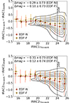 |
Fig. A.1. Difference between the magnitudes derived in this work and the ones in the Cosmic Dawn Catalogue. The black contours show the distribution of all sources in common between the two catalogues (from 10% to 90% of the sample), and red squares and yellow circles show the average values in magnitude bins for the EDF-N and EDF-F, respectively. We report in the top left the mean and standard deviation of the difference in magnitude in the two fields. We report results for the IRAC1 filter on the top and the IRAC2 filter on the bottom panel. |
Appendix B: Redshift recovery
The Euclid pipeline, at the moment, lacks LRD templates. This can have a direct impact on the redshift estimation for these objects. We therefore decided to test the redshift recovery for LRDs by simulating Euclid observations of LRDs and input this mock photometry to the Euclid pipeline.
In particular, we start by simulating simple LRD spectra, using two power laws, with red and blue continuum slopes at rest-frame optical and UV wavelengths. For the βUV and βopt continuum slopes, we considered the values measured by Kocevski et al. (2025) for a sample of 341 LRDs at z = 2–11, but with a median redshift of z = 6.4. We used these mock LRDs as templates, moving them from z = 1 to z = 7.6, where we have enough bands to measure the two slopes in all EDFs. We scale their absolute UV magnitudes (MUV) and compare these with the Euclid observational depths. We then derive photometric redshift, considering the same setup used in the Euclid pipeline.
In the top panel of Fig. B.1 we report the comparison between the recovered and input redshifts. As can be seen, the first effect is a bimodal distribution, with some galaxies that are wrongly placed at z < 2. In addition, the output redshift tends to be overestimated for galaxies at zinput < 2, and the upper limit at z = 6 naturally underestimate the redshift of z > 6 sources. Overall, we have about 40% of outliers (fout), defined as galaxies with |δz|=|zoutput − zinput|/(1 + zinput) > 0.15. If we remove these outliers, we obtain a distribution consistent with no redshift bias, since δz = 0.02 ± 0.07.
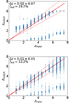 |
Fig. B.1. Redshift recovery using the Euclid pipeline (top) and with the double power-law fit improvement (bottom). In the upper right of each panel we report the fraction of outliers, defined as objects with |δz|=|zoutput − zinput|/(1 + zinput) > 0.15, the mean and standard deviation of δz, measured after removing the outliers. |
In the bottom panel of Fig. B.1 we instead show the comparison between the true redshift and the one recovered by fitting the mock photometry with a double power law and leaving the redshift free to vary (see Sect. 3). In this fit, we considered the pipeline redshift as a starting point and the uncertainties as limits. We verified that leaving the redshift totally free improves the results. This refinement in the redshift produces a substantial reduction in the outlier fraction, more than halving it (fout = 12%). At the same time, the biases at the different redshifts are similar and the z = 6 upper limit is removed. The expected mean redshift bias, after removing the outliers, is also slightly improved, becoming δz = 0.01 ± 0.05.
By comparing the intrinsic redshift distribution and the one derived after the two power-law fit, we derived an average redshift correction to apply to the estimated luminosity function (Sect. 4.3). These redshift corrections are derived in redshift bins and are: 0.60 at z = 1.0–1.5; 0.91 at z = 1.5–2.0; 1.32 at z = 2.0–2.5; 1.09 at z = 2.5–4.0; and 1.09 at z = 4.0–6.0
Appendix C: Impact of slope uncertainties on sample selection
In this Section we focus on the impact of the uncertainties of the rest-frame UV and optical slopes on the sample selection. In particular, we start from the subsamples of sources with S/N > 3 in more than four filters. We then randomise the rest-frame UV and optical slopes 100 times, using a normal distribution centred on the best value and with standard deviation equal to the respective uncertainties. After this randomisation, we select for each iteration the number of v-shape sources, checking then the subsample of these objects that is also compact, is not contaminated by nebular emission lines and has a χ2 < 100. We do not perform the visual check of all sources selected in the different iterations.
In Table C1 we report the 16% and 84% of the distribution of the number of selected objects in the different fields. As visible, the values are larger than the one reported in Table 3, indicating that the number of LRD candidates may be underestimated due to the uncertainties on the rest-frame UV and optical slopes. Because the number of potential contaminants is expected to be larger than the number of LRD, however, we prefer to keep the conservative estimates derived in the main text of this work.
16% and 84% percentages of the number of selected objects when randomising the slope measurements.
Appendix D: Complete sample
In Table D1 we include the final list of LRD candidates and their properties, derived using the double power law fit described in Sect. 3 and whose performance is shown with mock data in Appendix B.
Properties of LRD candidates.
Appendix E: Observed properties of the LRD candidates
In Fig. E.1 we report the photometric redshift distribution for the three fields. The average redshift is similar among the three fields and is z = 1.7. The average redshift of IRAC-detected LRD candidates is larger, that is z = 2.4, with no LRD candidates at z ≥ 4.
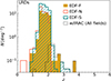 |
Fig. E.1. Photometric redshift distribution of the samples of LRD candidates in the three EDFs. The dotted black histogram shows the overall distribution of sources detected in IRAC. |
In Fig. E.2 we report the magnitude distributions in the four Euclid filters, showing that they are similar for all three fields, with the EDF-N having a light excess at bright magnitudes with respect of the other two fields. Indeed, the mean magnitudes in the EDF-F and EDF-S differ by less than 0.1 mag, and the EDF-N shows slightly brighter magnitudes than the other two fields, with a difference below 0.3 magnitudes. The similarities in the magnitude distributions of the three fields reassures us that the selection is reasonably uniform across these fields.
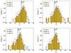 |
Fig. E.2. Magnitude density distribution of the LRD candidates in the three fields in the four Euclid filters. The vertical solid and dashed black lines indicate the 10σ and 5σ depths, respectively. |
LRD candidates have mean magnitudes of IE = 25.5, YE = 24.3, JE = 24.0, and HE = 23.7 and hence are relatively faint. Indeed, only 11% and 8% of them have magnitudes brighter than the 10σ depth in the HE and IE filters, respectively, and these fractions decrease to 7% and 3% in the JE and YE filters. The sources detected in IRAC have a mean magnitudes of IRAC1 = 22.2 and IRAC2 = 21.5, showing that they are relatively bright in these two filters. In general, the fit is based only on four filters with S/N > 3 for 20% of the sample, and the remaining sources have from five to 10 filters with S/N > 3.
Appendix F: Comparison with other Euclid AGN catalogues
As mentioned in Sect. 4.2, we verified the overlap between our sample of LRD candidates and other AGN catalogue derived using Q1 data. We give here more information on the criteria used in these other paper, their completeness, purity and level of overlap with our sample.
Appendix F.1: Optical photometric selections
The first selection presented in Euclid Collaboration: Matamoro Zatarain et al. (2026), named B24A, is based only on two Euclid colours and was presented in Euclid Collaboration: Bisigello et al. (2024). Taking into account the limitations of this colour selection, since it has a low purity (P = 0.166 ± 0.015) and a low completeness (C = 0.347 ± 0.004), 254 (8%) of our LRD candidates could be classified as QSO candidates. The selection is indeed based on the IE − JE and IE − YE colours, so it could trace the blue UV rest-frame slope, which is present in LRDs and blue QSOs, but missing the red optical rest-frame slope.
The presence of observations in the u band in the EDF-N allows us to use an additional colour selection from Euclid Collaboration: Bisigello et al. (2024), applied again by Euclid Collaboration: Matamoro Zatarain et al. (2026). The selection, which we refer to as B24B, is based on the u − z and IE − HE colours, corresponding to a completeness of C = 0.861 ± 0.004 and a purity P = 0.992 ± 0.017. Of the entire sample of LRD candidates in the EDF-N, 258 (26%) are selected by the B24B selection.
In addition, Euclid Collaboration: Matamoro Zatarain et al. (2026) identified two new colour selections fine-tuned based on the colours occupied by DESI QSO. A first selection is based on Euclid colours (IE − YE and JE − HE) and a compactness criteria, and the second include also ground-based ancillary colours (g − z and IE − HE). We refer to this selections as MZ25a and MZ25b, respectively. The first selection incudes 1686 QSO candidates, corresponding to 50% of our catalogue, and the second criteria selects 1939 QSO candidates, corresponding to 58% of our catalogue.
The official Euclid catalogue (Euclid Collaboration: Tucci et al. 2026) includes also a probability of being a QSO, obtained by performing a supervised machine learning method called Probabilistic Random Forest (PRF, Reis et al. 2019), trained using photometric data only. Using this classification, Euclid Collaboration: Matamoro Zatarain et al. (2026) identified QSO as objects having a QSO probability above 85% and not being classified as stars. Of our sample, 34 (1%) LRD candidates are also classified as QSO using this method.
None of our LRD candidates are in the purified subsets of the Gaia QSO candidates catalogue (see Sect. 3.2.4. in Euclid Collaboration: Matamoro Zatarain et al. 2026) based on the Data Release 3 (DR3, Gaia Collaboration 2023) or in the machine-learning classification based on Euclid images by Euclid Collaboration: Margalef-Bentabol et al. (2026).
Appendix F.2: Near-IR photometric selections
Taking advantage of the WISE coverage, Euclid Collaboration: Matamoro Zatarain et al. (2026) also applied the two photometric selections by Assef et al. (2018). With the selection corresponding to 75% completeness, called A18C75, 35 (1%) of the LRD galaxies are identified as potential QSOs. With the selection corresponding to 90% reliability, called A18R90, only four LRD candidates are also QSO candidates.
In addition, given that IRAC observations are available for at least part of the sample, we verify if any of our LRD candidates satisfy the AGN selection by Donley et al. (2012). Unfortunately, in the EDF-S this selection can not be applied, as there are observations only on two IRAC bands. In the other two fields, only two LRD candidates has a S/N>3 in all four IRAC filters and these objects are inside the selection criteria by Donley et al. (2012).
Appendix F.3: Spectroscopic selections
The EDF-N is partially covered by DESI EDR (DESI Collaboration 2024), allowing for the classification of QSOs using spectroscopic data. This classification is also included in Euclid Collaboration: Matamoro Zatarain et al. (2026, Sect. 3.3.1) and two LRD candidates (0.2% of our sample in the EDF-N) are indeed classified as QSOs by the DESI spectral type classification and looking at the DESI spectra, having FWHM ≥ 1200 km s−1 in one of the hydrogen lines. Euclid Collaboration: Matamoro Zatarain et al. (2026) also includes other diagnostic based on spectroscopic DESI spectra, but no LRD candidates are selected by them.
Appendix F.4: X-ray AGNs
We now compare our catalogue with the Euclid X-ray selected AGN catalogue (Euclid Collaboration: Roster et al. 2026). This catalogue lists the most likely Euclid counterparts to the 4XMM DR13, Chandra CSC 2.0, and eROSITA DR1 catalogue. While the former two cover the three Euclid field in a few, deep pointed observations, the latter covers EDF-F and EDF-S homogeneously but at a shallow depth (see figures 1 and 2 of Euclid Collaboration: Roster et al. 2026).
Out of the entire sample of LRD candidates, three sources (0.09%) are present in the Euclid X-ray selected AGN catalogue, two in the EDF-S and one in the EDF-F. The two sources in the EDF-S are matched with sources in the eROSITA DR1, with a probability of being the right counterparts of pany = 0.16 and 0.97. The source in the EDF-F is matched with a X-ray source in the Chandra CSC 2.0 catalogue with a probability of being the right counterparts of pany = 0.98. For these sources the chance association can be higher than 80% (see Fig. 7 in Euclid Collaboration: Roster et al. 2026). Out of the three matches, only one has S/N > 3 at (0.5–2.3) keV, that is f0.5−2.3 kev = (3.92 ± 1.08) × 10−14 erg s−1 cm−2, corresponding to a luminosity of 2.61 × 1044 erg s−1 at of zphot = 1.1. A second source has instead a S/N = 2 at (0.5–2.3) keV, that is f0.5−2.3 kev = (1.24 ± 0.62) × 10−14 erg s−1 cm−2, and the third one is below S/N < 1, with a 3σ upper limit of f0.5−2.3 kev = 5.06 × 10⁻¹⁶ erg s−1 cm−2.
Euclid Collaboration: Roster et al. (2026) also identify potential X-ray emitters, using a combination of Bayesian statistics and machine learning. This classification allows us to identify potential X-ray emitters outside the area covered by X-ray observations, which may be useful, for example, for follow up studies. There are 73 LRD candidates that are classified as potential X-ray emitters.
Overall, the small fraction of X-ray LRD candidates of this work is in line with previous works, showing that the majority of LRD are X-ray weak (e.g. Yue et al. 2024), but it is necessary to consider that the X-ray surveys considered here are shallower than the one used to matched previous LRDs selected with JWST. Further analysis of the X-ray emission of these sources in the future could shed light on the AGN contribution in LRDs.
A reassuring result is that all X-ray LRDs have a probability of less than 1% of being Galactic sources. This probability was derived by Euclid Collaboration: Roster et al. (2026) using a random forest algorithm trained on the methodology described in Salvato et al. (2022).
All Tables
Area coverage in deg2 of the available IRAC images (Euclid Collaboration: Moneti et al. 2022).
Number of sources retrieved in the different steps of the LRD selection in the three EDFs.
16% and 84% percentages of the number of selected objects when randomising the slope measurements.
All Figures
|
Fig. 1. Redshifts in which the different Euclid, IRAC, and ground-based filters trace the optical (red bars) or UV (blue bars) continuum. The grey shaded area indicates the redshift range in which we have at least four filters to derive the slopes necessary to select LRDs. The hatched area indicates the redshift range covered without IRAC. The first two bars, separated by a horizontal solid black line, indicate the redshift range in which at least two JWST NIRCam broad-band filters trace the rest-frame optical or UV continuum. |
| In the text | |
|
Fig. 2. Two example LRD candidates, showing cutouts of 4″ × 4″ in the four Euclid filters and the two shortest IRAC channels. From left to right: IE, YE, JE, HE, IRAC1, and IRAC2. We report the size of the PSF in the top left and the physical scale on the bottom left corner of each panel. |
| In the text | |
|
Fig. 3. Fit with two power-laws of the photometric data of the two example LRD candidates shown in Fig. 2. We show fluxes with S/N > 3 as black squares, and the 3σ upper limits are shown with empty triangles. The best fit is shown with a blue solid line, and the shaded region shows the 16% and 84% uncertainties. We report the χ2 and the output parameters in the top left corner. |
| In the text | |
|
Fig. 4. MUV and redshift for all LRD candidates, shown as contour lines, equally spaced from 10% to 90%. The last line represents 99% of the distribution. The remaining 1% of the sample is shown with stars, colour-coded based on their field. We also show three samples of LRDs selected with JWST observations (Kocevski et al. 2025; Labbé et al. 2023; Kokorev et al. 2024a; Akins et al. 2024). The dotted black line shows the 80% completeness that is expected when the EDFs are at their final depth. |
| In the text | |
|
Fig. 5. Top: Half-light ratio in the JWST/F444W filter vs. redshift for the sample of extended v-shape objects by Kocevski et al. (2025). The horizontal solid line indicate the HE band FWHM, scaled assuming a Gaussian function. Bottom: Fraction of extended v-shape objects that is expected to be unresolved in the HE band as a function ofredshift. |
| In the text | |
|
Fig. 6. UV luminosity function of the LRD candidates from z = 0 (top left) to z = 4 (bottom right). The empty stars indicate the values before any corrections, and the coloured stars show the density after correcting for completeness and redshift estimation. The coloured triangles show the conservative estimation derived considering only IRAC-detected sources. The vertical shaded black regions show the range of the 80% completeness in the three fields. In the top left corner, we report the number of objects inside the redshift bin, and we show the number of IRAC-detected sources in the bin in brackets. The empty symbols show UV luminosity functions of QSOs from Giallongo et al. (2012, and reference therein), Akiyama et al. (2018), and Pan et al. (2022). We also report the UV luminosity function of QSOs modelled by Kulkarni et al. (2019, dashed black line). For a comparison, the horizontal dash-dotted red line shows the minimum density probed by the HST CANDELS survey (0.29 deg2Grogin et al. 2011; Koekemoer et al. 2011), and the horizontal dotted red line shows the minimum density probed by the JWST COSMOS-WEB survey (0.54 deg2 Casey et al. 2023). |
| In the text | |
|
Fig. 7. Comparison of the corrected UV luminosity function of LRD candidates from z = 0 to z = 4, and values at z = 6 from the literature (Kocevski et al. 2025; Kokorev et al. 2024a). |
| In the text | |
|
Fig. A.1. Difference between the magnitudes derived in this work and the ones in the Cosmic Dawn Catalogue. The black contours show the distribution of all sources in common between the two catalogues (from 10% to 90% of the sample), and red squares and yellow circles show the average values in magnitude bins for the EDF-N and EDF-F, respectively. We report in the top left the mean and standard deviation of the difference in magnitude in the two fields. We report results for the IRAC1 filter on the top and the IRAC2 filter on the bottom panel. |
| In the text | |
|
Fig. B.1. Redshift recovery using the Euclid pipeline (top) and with the double power-law fit improvement (bottom). In the upper right of each panel we report the fraction of outliers, defined as objects with |δz|=|zoutput − zinput|/(1 + zinput) > 0.15, the mean and standard deviation of δz, measured after removing the outliers. |
| In the text | |
|
Fig. E.1. Photometric redshift distribution of the samples of LRD candidates in the three EDFs. The dotted black histogram shows the overall distribution of sources detected in IRAC. |
| In the text | |
|
Fig. E.2. Magnitude density distribution of the LRD candidates in the three fields in the four Euclid filters. The vertical solid and dashed black lines indicate the 10σ and 5σ depths, respectively. |
| In the text | |
Current usage metrics show cumulative count of Article Views (full-text article views including HTML views, PDF and ePub downloads, according to the available data) and Abstracts Views on Vision4Press platform.
Data correspond to usage on the plateform after 2015. The current usage metrics is available 48-96 hours after online publication and is updated daily on week days.
Initial download of the metrics may take a while.