| Issue |
A&A
Volume 699, July 2025
|
|
|---|---|---|
| Article Number | A53 | |
| Number of page(s) | 11 | |
| Section | Planets, planetary systems, and small bodies | |
| DOI | https://doi.org/10.1051/0004-6361/202453584 | |
| Published online | 30 June 2025 | |
The Io plasma torus observed by Juno between 2016 and 2022
Results from the Io footprint position and the Io plasma torus radio occultations
1
Laboratory for Planetary and Atmospheric Physics, Space Sciences, Technologies and Astrophysical Research Institute, University of Liège,
Liège,
Belgium
2
Institute for Space Astrophysics and Planetology, National Institute for Astrophysics (INAF-IAPS),
Rome,
Italy
3
Department of Industrial Engineering, Alma Mater Studiorum – Università di Bologna,
Italy
4
Centro Interdipartimentale di Ricerca Industriale Aerospaziale, Alma Mater Studiorum – Università di Bologna,
Italy
5
Aix-Marseille Université, CNRS, CNES, Institut Origines, LAM,
Marseille,
France
★ Corresponding author: alessandro.moirano@uliege.be
Received:
22
December
2024
Accepted:
29
April
2025
Context. The Io plasma torus (IPT) is a dense, toroidal plasma cloud around Jupiter, approximately centered on Io’s orbit. Iogenic volcanic activity supplies material to the IPT, mainly through direct outgassing or sublimation of frozen volcanic sulfur dioxide. Material from the IPT diffuses outward into an extended plasma disk, whose electric currents generate a strong magnetic field. This field, together with the internally driven planetary magnetic field, contributes to a powerful and highly variable magnetospheric environment. Because the plasma disk is supplied by the IPT, monitoring its condition and variability is essential for understanding the dynamics of the magnetosphere and to estimate potential hazards for deep space missions.
Aims. This study aims to constrain the average IPT conditions between 2016 and 2022 using observations of the auroral footprint of Io and radio occultations of the IPT conducted by the Juno orbiter. In addition, we investigate density and temperature variations occurring over timescales of weeks to a few months.
Methods. We computed the IPT’s plasma distribution using a diffusive equilibrium, force-balance model. This model simulated both the position of the Io footprint observed in the infrared and ultraviolet and the induced path delay in the radio-tracking data recorded by the Deep Space Network. The advantage of this approach is the ability to break the parameter-space degeneracy that arises when analyzing the two types of observations individually.
Results. We conclude that, between 2016 and 2022, the IPT temperature was 80−50+100 eV, and the electron density was 3000±1400 cm−3.
Key words: planets and satellites: aurorae / planets and satellites: magnetic fields
© The Authors 2025
 Open Access article, published by EDP Sciences, under the terms of the Creative Commons Attribution License (https://creativecommons.org/licenses/by/4.0), which permits unrestricted use, distribution, and reproduction in any medium, provided the original work is properly cited.
This article is published in open access under the Subscribe to Open model. Subscribe to A&A to support open access publication.
1 Introduction
Jupiter’s magnetosphere hosts powerful and complex electromagnetic processes, primarily driven by its strong magnetic field, rapid planetary rotation (∼10 hours per Jovian day), and high plasma density. The peak electron density in Jupiter’s magnetosphere can reach 2000-3000 electrons cm−3, in contrast to the typical ∼1 cm−3 in the terrestrial magnetosphere. This dense plasma consists mainly of oxygen and sulfur, with a minor fraction (∼1-10%) of protons and sodium. The presence of a volcanically active moon around Jupiter - Io, whose volcanism is driven by tidal stress with Jupiter (Peale et al. 1979) - has a major role in shaping the structure and dynamics of the Jovian magnetosphere. Io primarily outgasses sulfur dioxide (SO2) and sodium chloride (NaCl). Sulfur dioxide mostly freezes on the surface of the moon and then sublimates, while NaCl disperses directly around the moon, forming a relatively dense and stable atmosphere (Roth et al. 2020). The interaction between Io and the plasma in the Jovian magnetosphere dissociates and ionizes Io’s atmosphere, leading to a diffuse neutral cloud around Io and a dense plasma torus (electron density ∼2000-3000 cm−3) approximately around Io’s orbit, known as the Io plasma torus (IPT; Bagenal & Dols 2020). When a new ion forms in Io’s rest frame, it is “picked up” by the electric field generated by its motion relative to the magnetic field and is accelerated toward rigid corotation with Jupiter. The centrifugal force, plasma pressure, magnetic confinement, and radial diffusion determine the plasma density distribution in the IPT. Due to the relative tilt between Jupiter’s spin axis and its magnetic dipole (approximately ten degrees, Connerney et al. 2022), the centrifugal equator of the IPT is tilted by about two-thirds (Hill et al. 1974), or approximately seven degrees from the spin axis. Plasma diffuses outward from the Io torus and forms an extended plasma disk around Jupiter between 6-8 RJ (1RJ = 1 equatorial Jovian radius = 71 492 km) and ∼50 RJ (Huscher et al. 2021). The magnetic field generated by the plasma disk (commonly referred to as the “external field”, in contrast to the “internal field” which originates in the planet’s interior) is fundamental in determining the size and compressibility of the entire magnetosphere, as its magnitude is similar to that of the internal field (Connerney et al. 2020). Consequently, the presence of the dense plasma disk inflates the Jovian magnetosphere, roughly doubling its size. The plasma disk is affected by the intrinsic variability of the plasma source from Io and the IPT (Yoshioka et al. 2018). Therefore, monitoring the IPT is essential for both scientific and operational purposes. Understanding the complex chain of processes that brings material from Io’s interior to Jupiter’s magnetosphere requires insights from a wide range of astrophysical fields, including geology, chemistry, electrodynamics, celestial mechanics, plasma physics, and fluid dynamics. Ideally, this necessitates simultaneous and continuous monitoring of several environments, such as the level of volcanic activity on Io, the condition of Io’s atmosphere and ionosphere, the IPT, the neutral cloud near Io, and the solar wind. The ability to constrain IPT conditions over several years is for supporting ongoing observations by Juno (Bolton et al. 2017), as well as ground-based observations that aim to unravel the interplay between Io, the torus, Jupiter, and its magnetosphere. Moreover, the rich and ever-evolving magnetosphere of Jupiter creates a hazardous and sometimes unpredictable environment (e.g., Greathouse et al. 2022), where radiation can hinder the success of deep space missions around Jupiter. As the Jupiter Icy Moons Explorer (Juice) and Europa Clipper missions are expected to reach Jupiter in 2031 and 2030, respectively, with a focus on the Galilean moons, it is fundamental to improve our understanding of local conditions near the moon and their expected variability. This knowledge is necessary to avoid or minimize undesired instrument saturation, safe-mode switching, and radiation damage, and to maximize the scientific output of these missions.
To derive the bulk parameters of the plasma distribution within the IPT (namely, density and temperature), we use two datasets gathered by the Juno spacecraft between 2016 and 2022: the position of the auroral emission associated with the orbital motion of Io (Hue et al. 2023; Moirano et al. 2024) and radio occultations of the IPT from radio-tracking systems (Moirano et al. 2021; Phipps et al. 2021). Figure 1 illustrates the observational geometry for both measurement types. The Io footprint (IFP), which refers to Io-related auroral emission, originates from the relative velocity between Io, which orbits with a period of ∼42.5 hours, and the IPT plasma, which exhibits near-rigid corotation with Jupiter with a period of ∼10 hours (Connerney et al. 1993; Prangé et al. 1996; Clarke et al. 1996). This velocity difference generates a local perturbation in the plasma flow, which propagates away from Io as Alfvén waves, and travels down Jupiter’s magnetic field lines to its ionosphere (Neubauer 1980). Since Alfvén speed depends on both the magnetic field and plasma density, the IFP position encodes information about these two quantities. The magnetic field around Io’s orbit is dominated by the internal field, hence it can be safely considered constant over a timespan of decades, and variations in the IFP position observed over weeks or months should be attributed to IPT density changes (Hue et al. 2023; Moirano et al. 2023). Due to the high plasma density in the torus and the approximate seven-degree tilt between Io’s orbit and the IPT’s centrifugal plane, Alfvén waves take 2-14 minutes to propagate from Io to Jupiter, depending on the moon’s longitude (Hinton et al. 2019; Hue et al. 2023; Moirano et al. 2023). Consequently, the auroral emission of the IFP typically occurs downstream (relative to the plasma flow past Io) with a delay dependent on Io’s centrifugal latitude and the IPT density distribution along the magnetic field. Through inversion, we can infer the Io torus conditions from the IFP position, which is itself determined by the delay in the propagation of the Alfvén waves from Io to Jupiter. This concept has been applied to explain the variable distance between the spots of the Ganymede footprint, suggesting that these variations reflect plasma disk conditions (Bonfond et al. 2013). Footprint position inversion has recently proven useful for quantifying variations in IPT conditions (Moirano et al. 2023), as well as in the plasma disk at Europa’s orbit (Satoh et al. 2024), although plasma temperature and density remain degenerate and cannot be determined individually unless one parameter is constrained. To resolve such degeneracy, we combine Juno’s IFP position with radio occultations conducted near perijove (PJ), a term also used to refer to individual Juno orbits, numbered for specificity). Figure 1 schematically illustrates how the two instruments probe the IPT during each PJ. The radio signals used to track the spacecraft position and velocity experience frequency shifts due to the IPT’s dispersive properties. This shift is proportional to the time derivative of the total electron content (TEC) between Juno and the ground station (Bertotti et al. 1993). By integrating the measured frequency shift, we obtain the TEC, providing an additional constraint on the plasma density distribution of the IPT. Juno’s north-south trajectory enables near-vertical radio occultation scans of the IPT, allowing sampling of the plasma’s vertical distribution, which depends on the plasma temperature. In contrast, the TEC reported by Juno depends on the local plasma density and radial extent of the torus. Because IPT occultations and IFP observations occurred within hours of each other, during multiple PJs between 2016 and 2022, we aim to constrain the average plasma density and temperature of the IPT over the same period by combining these two types of measurements. Additionally, we investigate IPT variability by comparing the two datasets for individual Juno orbits.
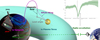 |
Fig. 1 Overview of Io torus monitoring by Juno. The position of the Io footprint is observed by the Jovian Infrared Auroral Mapper (red field of view) and/or the Ultraviolet Spectrograph (blue field of view) as the spacecraft passes over the polar regions. The lead angle (gray arrow) represents the angular difference between the Io footprint’s longitude, mapped at Io’s orbit using the magnetic field (black dashed line), and Io’s longitude at the same epoch. The lead angle encapsulates information about the tilt of the Alfvén wing (purple line; see Section 3) relative to the magnetic field, and thus about the condition of the torus. Between polar overflights, Juno frequently performs radio occultation of the Io torus (green line), conducted by the Ka-band Translator System and Small Deep Space Transponder of the Gravity experiment onboard the spacecraft. The path delay measured by the Deep Space Station (plot on the right) shows a pronounced signature caused by the electron content of the Io torus as Juno passes behind it. |
2 Observations and data reduction
Since 2016, the Juno mission has orbited Jupiter in a highly eccentric polar orbit, making its closest approach approximately every 50 days and providing a unique vantage point for observing auroral polar regions. The spacecraft is equipped with two remote sensing instruments (excluding JunoCam, which was unused here due to the lack of IFP observations): the Jovian Infrared Auroral Mapper (JIRAM, Adriani et al. 2017) and the Ultraviolet Spectrograph (UVS, Gladstone et al. 2017). The former is a 128 × 432 pixel imager that captures snapshots using a bandpass filter spanning 3.3-3.6 microns and an angular resolution of ∼0.01 degrees, corresponding to a few tens of kilometers at the Jovian surface (which is usually the 1-bar pressure level). The wavelength range optimizes the contrast between the sunlit planetary disk and the emission from the H3+ ion. This ion forms through reactions between H2 and H2+, the latter generated by ionizing electron precipitation associated with the aurora (Miller et al. 2020). H3+ is destroyed either by electron recombination at high altitudes (above ∼500 km from the surface) or through reactions with atmospheric hydrocarbons at low altitude. These hydrocarbon reactions are so effective that any H3+ emission from below the methane homopause is completely suppressed. JIRAM required a one-second exposure time to obtain a clear picture of the aurora. Since Juno rotates with a period of ∼30 seconds, the instrument captures up to one image per rotation. Additionally, JIRAM uses a de-spinning mirror to lock-on to the target during the exposure time to avoid smearing. However, a technical anomaly of the mirror mechanism halted auroral observations starting from PJ 43. Thus, this study uses data from Juno’s first 42 orbits. Images acquired in the L-band suffered significant interference from the adjacent M-band filter, which completely obscured any signal near the filter junction. To compensate, we applied an exponential correction to each image (Mura et al. 2017) and discarded the first 38 rows. Although this correction affects the absolute image brightness, it does not change the emission morphology, and thus the results of this study remain unaffected. The IFP positions in the JIRAM images were sourced from the supporting information of Moirano et al. (2024), who used a 2D peak-finding algorithm (Natan 2021) to determine the location of the peak emission.
Juno-UVS is a spectrograph operating between 68 and 210 nm, with most auroral emission detected between ∼120 and ∼170 nm. It achieves an angular resolution of up to ∼0.1 degrees (Greathouse et al. 2013). The auroral emission detected by Juno-UVS primarily arises from Lyman-alpha and Lyman and Werner bands (e.g., Badman et al. 2015). Although UVS has a spatial resolution approximately one order of magnitude lower than JIRAM, it offers superior spatial coverage due to a scan mirror that enables its field of regard to shift up to ±30 degrees from Juno’s spin plane. JIRAM has been unable to observe the IFP in both hemispheres or during every Juno orbit due to operational constraints. Therefore, UVS data filled the observational gaps left by JIRAM, although at a lower spatial resolution.
Juno is also equipped with two radio tracking subsystems-the Ka-Translator System (KaTS) and the Small Deep Space Transponder (SDST) - which are used by the gravity experiment to accurately determine the spacecraft’s velocity (Asmar et al. 2017). The experiment employs a two-way, dual link. By using Deep Space Network (DSN) ground stations instead of an onboard oscillator, instrumental stability and technological complexity requirements are transferred to the ground, making maintenance easier and improving accuracy. Two frequencies are required to almost fully calibrate nondispersive contributions to the frequency shift (e.g., those due to the Doppler shift; Mariotti & Tortora 2013) and to isolate the dispersive shift caused by IPT plasma (Moirano et al. 2021; Phipps et al. 2021). Near each PJ with a planned gravity measurement, a radio transmission is sent from Earth, in the X band in both channels (∼7.2 GHz) or in the X and Ka bands (∼34.4 GHz), depending on the availability of the Deep Space Station (DSS) 25 of the DSN. The incoming frequency is slightly shifted onboard by the spacecraft (∼8.4 GHz and ∼32.1 GHz for the X and Ka bands, respectively) to avoid interference between the uplink and the downlink, before the signal is relayed back. Plasma between Juno and the ground stations affects the path delay between the two channels, requiring calibration and inclusion of these contributions in the final uncertainty estimates. The delay caused by Earth’s ionosphere is corrected using GPS data (Thornton & Border 2000). Its electron content uncertainty depends on the elevation angle at the ground station and is estimated as 2.5 TECU/sin(θ), where 1 TECU = 1016 m−2, and θ is the elevation angle at the tracking DSS. This 2.5 TECU value is the approximate uncertainty of the terrestrial ionosphere at mid- and low latitudes, as estimated by the Space Weather Prediction Center of the National Oceanic and Atmospheric Administration1. Solar wind scintillation is another source of uncertainty, which depends on the Sun-Earth-Probe (SEP) angle, and is computed by integrating the uncertainty in the X band frequency shift (Iess et al. 2014). After correcting for Earth’s ionosphere, path delay residuals remain alongside the IPT signature in Juno’s radio occultations. A static axisymmetric model of the solar wind (e.g., Köhnlein 1996) does not satisfactorily simulate such residuals, and the origin of these disturbances is currently unknown. Nevertheless, the IPT signature is clearly visible, suggesting that the path delay caused by the IPT dominates other contributions at certain times near each of Juno’s closest approaches to Jupiter. Under this assumption, Sect. 3.2 describes our approach for comparing the data with the model, taking into account the presence of background residuals.
Table 1 summarizes the observations used in this study. Of the 42 orbits considered, 25 reported a radio occultation, and the IFP was observed at least once by JIRAM or UVS during each PJ.
3 Methods
We used a 3D model of the IPT to simulate both the IFP position and the radio occultations, as described in the following sections. To this end, we used Voyager 1 plasma measurements of ion concentrations, electron density, and temperature near the centrifugal equator from Dougherty et al. (2017) as a reference for this work. This choice was motivated by the comprehensive and consistent dataset provided by Voyager 1, which served as input for modeling the plasma distribution of the IPT. We adopted a diffusive equilibrium force-balance model to extrapolate plasma density along the magnetic field lines from values at the centrifugal equator. This model includes the gravity and centrifugal forces, the pressure gradient along the magnetic field, the magnetic mirror force between the two hemispheres, and the ambipolar diffusion due to charge separation (Bagenal & Sullivan 1981; Mei et al. 1995). The model includes six ion species that represent the bulk of the plasma: S+, S2+, S3+, O+, O2+ and H+. Additionally, a fraction of suprathermal O+ was included in the mixture, following Voyager 1 observations. The radial profiles of electron density, temperature, and ion fractions at the centrifugal equator between 3 and 16 RJ are shown in Figure 2. These profiles were obtained by smoothing the Voyager 1 data to match the model’s spatial resolution, except the electron density and temperature outside 10 RJ, which were obtained by analytical approximations. We modeled the electron density in three IPT regions, along with decreasing exponential to simulate the density transition between the IPT and the plasma disk between 10 to 16 RJ :
![n(r)& =& \sum_1^2n_kexp\Bigg[-\Bigg(\frac{r-R_k}{W_k}\Bigg)^2\Bigg] \\ && +n_3exp\Bigg[-\Bigg(\frac{r-R_3}{W_3}\Bigg)^2\Bigg]S_3(r)+n_4exp\Bigg(-\frac{r-R_3}{W_3}\Bigg)S_4(r)](/articles/aa/full_html/2025/07/aa53584-24/aa53584-24-eq2.png) (1)
(1)
where k = 1, 2, 3, and 4 represent the three IPT regions (the inner disk, the ribbon, and the warm torus, respectively) and the IPT-plasma disk transition from inside out. The peak densities at the centrifugal equator of each region were nk = 1800, 3000, 2000, and 100 cm3, the peak positions were Rk = 5.2, 5.7. 5.9, and 8.5 RJ, and the radial extensions were Wk = 0.3, 0.1, 1.8, and 2.0 RJ. The functions S3(r) and S4(r) are step-like, defined as 1/2 + π−1 atan((r - Rd)/L), where Rd = 5.8 RJ and L = 0.01 RJ for the warm torus, and Rd = 8.5 RJ and L = 0.5 RJ for the transition region. At Io’s orbit, the temperature of the bulk ions was ∼100 eV, while the electrons and the hot oxygen were at ∼5 eV and 400 eV, respectively. The temperature of the thermal ions dropped steeply to ∼5 eV inside ∼5RJ, causing the IPT to be ∼0.1-0.2 R J thick in the innermost region and ∼1 RJ in the warm torus. To simulate the temperature increase observed from 10 to 16 RJ (Bagenal & Delamere 2011), we approximated the temperature by an increasing exponential of the form
 (2)
(2)
where RT = 10 RJ, WT = 5 RJ, and T10Rj is the Voyager 1-based temperature at 10 RJ. The temperature of the hot oxygen was assumed to be non-isotropic, with an anisotropy A=T⊥/T∥=6.5 (Crary et al. 1996), while the other species were assumed isotropic. The ion fractions varied noticeably between 4.5 and 8 RJ and were mostly constant outside this range. We also assumed that the chemical composition was fixed inside 4.5 RJ, although this region is currently less constrained by observations than the regions outside. Nevertheless, the low plasma density (<100 cm−3) inside 4.5 RJ had a negligible effect on the radio occultations.
The profiles shown in Fig. 2 were used as boundary conditions to solve the diffusive equilibrium equations:
![n_{\alpha}(s) &=& n_{\alpha0}exp\left[\frac{m_{\alpha}\Omega_J^2(\rho^2-\rho_0^2)}{2k_BT_{\alpha\parallel}}+\frac{m_{\alpha}}{k_BT_{\alpha\parallel}}GM_J\left(\frac{1}{r}-\frac{1}{r_0}\right)\right.\\ && \left.+\left(1-\frac{T_{\alpha\perp}}{T_{\alpha\parallel}}\right)ln\left(\frac{B}{B_0}\right)-Z_{\alpha}e\frac{\Delta\phi(s)}{k_BT_{\alpha\parallel}}\right]](/articles/aa/full_html/2025/07/aa53584-24/aa53584-24-eq4.png) (3)
(3)
where mα is the particle mass, ΩJ is the angular rotation of Jupiter, kB is the Boltzmann constant, Tα|| and Tα⊥ are the parallel and perpendicular temperatures, respectively, G is the gravitational constant, MJ is the Jovian mass, r and ρ are the distance from the planet center and spin axis respectively, B is the magnetic field magnitude, Zα is the atomic number (Zα = -1 for the electrons), Δφ = φ(S) - φ0 is the potential associated with the ambipolar electric field, and s is the distance from the centrifugal equator along the field line. The quantities denoted by "0" refer to the centrifugal equator. The centrifugal and gravitational terms (the first two terms on the right-hand side of Eq. (3)) were neglected for electrons due to their small mass. The mirror force (i.e., the third term on the right-hand side of Eq. (3)) was omitted for species with isotropic temperatures (i.e., where Tα|| = Tα⊥). The set of equations obtained by combining Eq. (3) for each species α was closed by the charge neutrality condition  , where ne and ni are the electron and ion density, respectively.
To simulate different density and temperature conditions in the IPT, we multiplied the electron density and ion temperature profiles in Fig. 2 by the scaling factors SD and ST, respectively. We used the resulting scaled profiles to solve Eq. (3) along magnetic field lines obtained from the Juno Reference Model up to orbit 33 (JRM33), including both the internal field and the external field associated with the plasma disk (Connerney et al. 2020, 2022; Wilson et al. 2023). We based the choice of this magnetic field model on the agreement between the IFP track observed by Juno and the predictions of this model (Moirano et al. 2024). We computed the magnetic field lines mapping to an equatorial region between 4 and 20 RJ using a fourth-order Runge-Kutta integration with a step of 0.1 RJ. To properly sample the small radial structure of the inner part of the torus, we separated the field lines mapping between 4.0 and 6.2 RJ by 0.05 RJ radially and by 0.5 RJ outside this region. Field lines were separated by 10 degrees in longitude. We investigated the SD-ST parameter space between 0.25 and 3, with a step of 0.25 (144 combinations). We chose this range of values based on the large variations reported in the literature: factors of 2-3 for temperature and ∼2 for density over timescales ranging from weeks to months (Delamere & Bagenal 2003; Morgan 1985; Morgenthaler et al. 2024; Thomas 1993). We computed the ion density using the electron density and ion fractions shown in Fig. 2.
Juno-JIRAM and Juno-UVS observations and radio occultations used to constrain the IPT in this study.
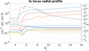 |
Fig. 2 Radial profiles of the IPT parameters at the centrifugal equator for the reference model based on Voyager 1: electron density (black dashed line), electron and ion temperatures (dot-dashed lines), and ion fractions (solid lines). |
3.1 Simulation of the lead angle of the Io footprint
We simulated the position of the IFP by computing the Alfvén travel time from Io’s orbit to Jupiter’s ionosphere at 600 km above the 1-bar surface, as this is the altitude where the infrared emission peaks (Moirano et al. 2024). We obtained the travel time by integration along the magnetic field:
 (4)
(4)
The Alfvén speed  , where μ0 is the magnetic permeability and ρ(s) is the ion mass density along the magnetic field line, approaches the speed of light in the high-latitude magnetosphere, and therefore required correction:
 (5)
(5)
Using the travel time Eq. (4), we constructed maps between Io’s position and the IFP position for the conditions given by each combination of SD and ST. For the Voyager 1 case, the Alfvén travel time varied periodically between 3 and 14 minutes, depending on Io’s centrifugal latitude. Using the Alfvén travel time Eq. (4), we computed the equatorial lead angle (Hess et al. 2010), defined as the angular separation Δλ between Io and the IFP position traced to Io’s orbit along the magnetic field. This quantity is proportional to the Alfvén travel time Eq. (4), and therefore also depends on the density distribution along the magnetic field passing near Io’s orbit:
 (6)
(6)
where Ωrel = ΩJ - ΩIo is the angular velocity of Io relative to Jupiter. The equatorial lead angle observed by both Juno-JIRAM and Juno-UVS exhibited a consistent sinusoidal dependence on Io’s longitude on average, although variability was also observed. Therefore, we used the average lead angle reported by Moirano et al. (2024) and Hue et al. (2023) to constrain the IPT parameter space, which can be considered as the average torus condition from 2016 to 2022. We also used orbit-by-orbit IFP observations to investigate specific orbits and deviations from the average torus. Using the simulated IFP maps, we computed the lead angle residuals between the Juno-based observations and our simulations. The parameter space constrained by this method was degenerate; that is, there was no unique combination of density and temperature for a given lead angle, since the travel time is approximately  , where Ti is the ion temperature (Moirano et al. 2023).
3.2 Simulation of the radio occultations
To better constrain the results obtained from the IFP lead angle, we applied the same IPT model to simulate the nearly simultaneous radio occultations (within a few hours). The theory underlying Juno’s radio occultations has been explained in previous studies (Phipps & Withers 2017; Moirano et al. 2021), and therefore we summarize only the general picture here. Due to dispersion by the plasma between Juno and the ground station, radio signals were received at a slightly different frequency f with respect to their original frequency f0 (Bertotti et al. 1993), and the fractional frequency y is related to the optical path by:
 (7)
(7)
In the high frequency approximation, the path delay Δl due to the dispersive property of the plasma was given by:
 (8)
(8)
where  , e is the elementary charge and the integral is along the line of sight γ between Juno and the ground station. The dual-frequency capability of Juno allowed us to decouple non-dispersive and dispersive contributions by taking linear combinations of the frequency shift in each channel (Mariotti & Tortora 2013). Due to the two-way nature of the link, the path delay was determined by both inbound and outbound transmissions, which, in general, were affected by different plasma conditions due to the ∼40 minutes light travel time between Earth and Jupiter. We assumed the IPT plasma contribution to be the same in both legs, as the time between the inbound and outbound crossing of the torus was ∼4 seconds. The different fractional frequency between the two radio channels is proportional to the time derivative of the TEC of the torus (Moirano et al. 2021):
 (9)
(9)
 (10)
(10)
The subscripts refer to the uplink and downlink frequency respectively, αij is the downlink-to-uplink frequency ratio, and Yij is the two-way frequency shift. Equation (10) was valid when there is no Ka uplink and the two channels used the X band; in this case, there was no uplink contribution to the frequency shift. To compare the path delay obtained by Juno with the IPT model, we performed a numerical integration of the electron density for different values of the same scaling factors SD and ST used to simulate the position of the IFP. We then converted the simulated TEC into path delay according to Eq. (8). Using Eqs. (7), (8), (9) and (10), we integrated the frequency shift measured by the DSN to obtain the observed path delay.
The solar wind, Earth’s ionosphere, and other plasma sources between the ground station and Juno affected the recorded path delay by adding terms to Eqs. (9) and (10). To properly compare the simulated path delay with the observations, we calibrated these contributions. This process was complicated by the periodic wiggling of the IPT around Jupiter’s spin axis, which sometimes moved the IPT plasma into the line of sight of the radio antennas while the spacecraft was still flying over the north pole. This “skimming occultation” occurred in the high-latitude, low-density regions of the IPT, making the isolation of the background plasma even more challenging and the determination of a precise IPT-occultation time window debatable. Nevertheless, the comparison between the path delay simulated with the reference IPT case and Juno’s observations showed a clear similarity in a 1-2 hour window around the spacecraft’s closest approach. This suggested that there was indeed a time window over which the IPT plasma was the main source of path delay. Therefore, for each PJ, we use the following procedure to remove the uncalibrated background delay. We used the reference model to estimate when the TEC was smaller than 25% of the peak value for each occultation, and we assumed that the IPT contribution in this time window was comparable or negligible with respect to other sources. If the time window to calibrate the background was less than 40% of the total path delay available for a single orbit, we discarded the radio occultation. For each SD-ST pair, we subtracted the model path delay from the observation and fit the background with a spline function (Reinsch 1967). The advantage of using a spline over a polynomial fit (e.g., Moirano et al. 2021; Phipps et al. 2021) was the flexibility to fit the variable background path delay, while avoiding large artificial fluctuations in the proper occultation that is removed from the fit. We used the reference model again to estimate when the TEC was greater than 50% of the peak value, and we assumed that the IPT contribution in this time window dominated over other sources. The cleaned data and the path delay simulated of each SD-ST pairs were compared over this time window, and we assessed the quality of the matching from the residuals. While approximate, this method allowed us to quantitatively compare data and model without assumptions on the nature of the unknown background disturbance in the path delay. Potential future improvements in the current understanding of this unknown source of path delay between Jupiter and the DSN will likely lead to further refinement of the present analysis.
To determine the best-matching torus conditions from both the lead angle and the radio occultations, we selected the SD-ST pair with the smallest χ2 among the 144 simulated cases:
 (11)
(11)
where νIFP and νocc are the degrees of freedom for 2 parameters (SD and ST), R are the residuals, and Δ is the measure uncertainty. Equation (11) represents the average of the reduced χ2 obtained from the lead angle and the radio occultations separately. The uncertainty on the lead angle accounted for both the size of the main auroral spot and the confidence in the average lead angle obtained from JIRAM and UVS observations (Hue et al. 2023; Moirano et al. 2024), which is ∼0.3 degrees. The main auroral spot has an approximate radius of 200 km (Moirano et al. 2024), approximately  degrees when mapping the IFP size at Io’s orbit along the magnetic field. In this study, we used
  as the uncertainty to compute the χ2 associated with the lead angle. The uncertainty on the path delay included both the measure uncertainty and the average residuals obtained from the background removal, which were computed for each orbit. The measurement uncertainty varied over time, primarily due to the changes in Juno’s elevation as seen from the ground station, but remained fairly constant around the peak of each occultation. The uncertainty used to compute the χ2 associated with the occultations was obtained by summing these two uncertainties, and ranged between
  = 23 mm (PJ 13) and 142 mm (PJ 23), with an average of53 mm. The lead angle residuals R
 were defined as the difference between the lead angle simulated with the model of Section 3.1 (e.g., panels b and c in Figure 3) and the average lead angle estimated from Juno observations (Moirano et al. 2024). The summation over i in Eq. (11) was performed over the data points used to compute the two curves. The radio occultation residuals R
 were obtained by taking the difference between the path delay simulated according to Section 3.2, and the path delay time series measured at the ground station. The summation over j was performed over the number of elements in the recorded time series, which had a sampling rate of 1 Hz. In this case, the number of observables corresponded to the length of the time series. At high centrifugal latitudes (i.e., large distances from the centrifugal equator), the Alfvén travel time of the wave traveling towards one hemisphere was far less sensitive to the IPT conditions than at the opposite hemisphere, as it crossed a smaller portion of the torus. Therefore, the observations of the IFP became less reliable when the travel time was short. To account for this, we multiplied a sinusoidal weight w
 to the lead angle residuals, where φ is Io’s longitude at the time of the observations, while φ0 = 20 and φ0 = 200 for observations in the northern and southern hemisphere, respectively. The values of φ0 were chosen according to the tilt of the magnetic dipole moment with respect to Jupiter’s spin axis towards ∼200 degrees (in System III longitude, which is the reference frame used in this work). The residuals of the radio occultation were instead weighted by wocc = 0.5(1-cos(SEP)). Small SEP value corresponded to Jupiter being near solar conjunction, where the solar wind contribution on the path delay was expected to be highest. Conversely, an SEP angle of ∼ 180 degrees corresponded to solar opposition, where the influence of the solar wind on the radio occultation was lowest.
To estimate the confidence levels, we computed Δχ2 =  , where
  is the minimum χ2, and we considered the three levels given by Δχ2 = 2.30, 6.18, and 11.8, which corresponded to 1σ, 2σ, and 3σ in a 2-dimensional parameter space (Press 2007).
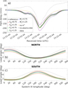 |
Fig. 3 Path delay recorded on 27 August 2016 between 11:50 and 15:50 UTC (gray line, panel a), and average IFP lead angle obtained by Juno between 2016 and 2022 (gray lines, panel b and c for the north and south pole, respectively) are shown alongside simulations obtained from the model described in Section 3. The thick black line corresponds to the Voyager 1-based reference case. Red lines show results for increasing or decreasing peak density of the warm torus, green lines show temperature and blue lines show radial extension (variations of 25% with respect to the reference case). Solid lines indicate a decrease and dashed lines an increase. The thin black line is obtained from same reference model with all the protons replaced by O+. The dot-dashed line is obtained by removing the plasma contribution from the transition between the IPT and the plasma disk. In panels b and c, the blue lines and the dot-dashed line overlap with the reference case. |
4 Results
The multi-species IPT described by Eqs. (1) and (3) depends on several parameters, so it is important to determine the effect of each parameter on the simulations presented here. First, we discuss the sensitivity of the IFP lead angle and path delay to the IPT parameters. We then present the best set of IPT parameters that match all Juno observations from PJ 1 to PJ 42, which we consider representative of the average torus conditions between 2016 and 2022.
4.1 Sensitivity analysis
Panel a of Figure 3 shows an example of the path delay signature obtained during PJ 1, along with the delay simulated from several conditions discussed here.
4.1.1 Density and temperature variations
Increasing or decreasing the peak density of the warm torus by 25% makes the signature proportionally deeper or shallower, effectively acting as a scaling factor. In contrast, temperature variations of 25% do not affect the peak of the delay but instead alter its wings, making the signature broader or narrower. Hence, in principle, density and temperature variations are nondegenerate parameters to retrieve. In practice, however, the relative tilt between the centrifugal equator and the Juno-Earth line of sight makes the two partially degenerate (Moirano et al. 2021).
4.1.2 Radial extent
The blue lines in Figure 3 are obtained from the IPT with the same peak density, but with a reduced or increased radial extent of the warm torus by 25%. These signatures are very close to those produced by a 25% increase or decrease in SD, and thus the signature of an extended or reduced torus is expected to be very similar to that of a denser or depleted torus. This similarity is not unexpected, as the TEC is obtained by integrating the density along the Juno-Earth line of sight, which is nearly parallel to the centrifugal equator.
4.1.3 Proton fraction
The radio occultations are remarkably sensitive to the presence of electrons along the wings of the path delay signature but less so at the peak. This is explained by the dependency of the path delay on the electron density, in contrast to the lead angle, which depends on the ion density and is weakly affected by protons (Moirano et al. 2023). Protons, owing to their low mass, can spread much farther from the centrifugal equator than heavier ions, carrying electrons with them. The “shoulders” visible before and after the occultation in Fig. 3 are caused by electrons associated with high-latitude protons, when the Juno-Earth line of sight becomes nearly tangent to the magnetic field lines connected to the ribbon and the inner part of the warm torus (i.e., the densest part of the torus). The diffusive equilibrium equations (Eq. (3)) assume that the temperature is constant along each magnetic field line; hence they are strictly valid only at low latitudes (within ∼20 degrees from the centrifugal equator due to temperature variations, e.g., Thomas & Lichtenberg 1997). Therefore, the plasma distribution and the path delay simulated at high latitude should not be compared quantitatively. Nevertheless, the electron density obtained in the reference case between 1 and 2 RJ is of the same order of magnitude as the values measured by Juno (Elliott et al. 2021; Huscher et al. 2021). We therefore retain the high-latitude simulation results to compare with the background and determine a suitable occultation time window.
4.1.4 Plasma disk
We investigated whether the presence of the plasma disk contributes to the path delay signature, as the disk extends over several tens of RJ, but with a density lower than that of the IPT. The dashed-dotted line in Figure 3 is obtained by turning off the density in the transition region between 10 to 16 RJ, revealing only a small decrease relative to the reference case. As with the IPT, the contribution of the plasma disk to the path delay is proportional to the peak density used in the model (100 cm−3). Therefore, a 2-3 factor increase in density in this region could make the plasma disk contribution non-negligible when determining the torus density. No direct measurements of the transition region are available to constrain any potential variability at the time of the observations. Thus, we assume that the plasma density scales with SD in the same way as the IPT, corresponding to densities between 50 and 250 cm−3.
The sensitivity of the IFP lead angle was discussed by Moirano et al. (2023), who used the same IPT model as the present study. The two most relevant parameters are the peak plasma density at the centrifugal equator and the ion temperature, represented by the SD and ST factors. The presence of temperature anisotropy is also important for the spatial distribution of the hot ions, although its precise value, which ranges from 3 to 10 for hot ions in the IPT (Crary et al. 1996), has little effect. This justifies fixing it at 6.5. Panels b and c of Figure 3 show the lead angle of Hue et al. (2023) and Moirano et al. (2024) compared to the lead angle simulated by varying the same parameters tested for the occultations. In agreement with Moirano et al. (2023), density and temperature are the most influential parameters overall, while the radial extension and the presence of the transition region have negligible effects on the lead angle. The variation in the lead angle is caused by the increased O+ that was arbitrarily added to conserve charge neutrality. Indeed, the Alfvén speed decreases near the centrifugal latitude where the oxygen ion density peaks (not shown), but not at high latitudes, where protons dominate.
4.2 The average Io plasma torus
Panels a and b of Fig. 4 show the lead angle χ2 for each SD-ST pair for the north and south poles, respectively. The minimum χ2 values are 1.1 and 1.2 for the northern and southern hemispheres, respectively. Small quantitative differences are observed between the two hemispheres, but the results are in broad agreement. As expected, the parameter space is degenerate, and the best model cases lie in a hyperbolic region given approximately by SDST = constant  . Interestingly, the reference case (that is, SD = 1 and ST = 1) is near the border of the best-matching region. This suggests that the IPT observed by Voyager 1 was less dense and/or colder than the average IPT during the Juno mission. Panel c of Fig. 4 shows the χ2 from the radio occultation, which has a minimum of 1.4 between SD = 0.75 and 2.00. The total χ2 in panel d of Figure 4 reaches a minimum of 1.6, corresponding to the region at SD = 1.50±0.7 and ST = 1.00
 . This suggests that the plasma parameters reported by Voyager 1 were likely near the lower end of the typical density and temperature of the IPT, at least according to the period covered in the present work.
The two χ2 values (lead angle and radio occultations) should be interpreted differently with respect to IPT variability. The lead angle χ2 is obtained by comparison with the fit to the lead angle observed by Juno, which can be considered the average lead angle. Therefore, any episodes of variability are smoothed out, and the lead angle χ2 in Fig. 4 should be considered strictly representative of the mean IPT. In contrast, the χ2 from the occultations is obtained by comparing the simulations with individual observations and is therefore affected by torus variability. For comparison, we computed the lead angle χ2 using Juno’s observation of the IFP instead of the sinusoidal average lead angle. The resulting parameter space agrees with that shown in Figure 4, but the minimum is broader. We believe that this further indicates the variability of the IPT and its effect on the residuals obtained in our analysis.
Figure 5 shows the χ2 values obtained by multiplying W3 in Eq. (1) (i.e., the radial extension of the warm torus) by 0.75 and 1.25 (panels a and b), by changing the protons into O+ (panel c), or by changing the thresholds used to determine the time window for background path delay calibration (panel d). The conversion of protons into oxygen ensures charge neutrality when analyzing the effect of protons on the radio occultations, but it also slightly affects the path delay, as discussed in Sect. 4.1. The minimum χ2 is obtained from SD = 1.75 and ST = 1.00
 when W3 is multiplied by 0.75, while SD = 1.25
 and ST = 1.25
 provide the best-match when W3 is multiplied by 1.25. This result arises from the degeneracy between nk and Wk in Eq. (1) when substituted into Eq. (8), which leads to Δl ∝ TEC ∝ nkWk. The best χ2 obtained by converting the protons into O+ corresponds to SD = 1.25
 and ST = 1.25
 . The decrease in density is unlikely to be caused by the addition of oxygen, as its effect on the path delay caused by the IPT is minimal (see Figure 3). Instead, as discussed in Section 4.1, the presence of protons strongly affects the wings of the path delay signature due to the occultation. The simulated delay is subtracted from the observations whenever it is less than 25% of the peak of the signature, before the spline smoothing is computed and calibrated. Therefore, we believe that the difference between the reference IPT and the simulation without protons may be ascribed to differences in background calibration between the two cases.
To test the effect of background removal, we reduced the threshold that determines the temporal window used for background calibration from 25% to 5%, and increased the comparison threshold used to compare observations and model from 50% to 75%. This approach ensures that the path delay measurements selected for background calibration are only weakly affected by the IPT, and the comparison is more sensitive to the details of the wings in the path delay signature. The drawback of using a smaller threshold is the reduction in the time window used to fit the background path delay, as well as the exclusion of certain PJs (15, 18, 22, 25, 29, 30, 33, 36, and 42) due to the absence of measurements unaffected by the IPT during the entire radio tracking segment, which prevents background calibration. Therefore, the following results should be considered less robust than those obtained with a less constraining threshold. The bestmatch density corresponds to SD values between 0.75 and 1.75, while the best temperature is obtained from ST > 0.5. To further investigate the effect of the temperature on the occultations, we estimate the parameter space using the same method as in panel d of Fig. 4, but without subtracting the IPT path delay before calibrating the background. The results (not shown) are very similar to the one shown in panel d of Figure 5.
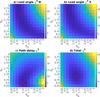 |
Fig. 4 χ2 values obtained by the IFP northern and southern lead angle (panels a and b, respectively), IPT radio occultations (panel c), and combination of both datasets (panel d). Red dots indicate the absolute minimum and magenta lines represent the 1σ, 2σ, and 3σ confidence levels. |
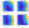 |
Fig. 5 χ2 obtained by combining the IFP lead angle by the IPT radio occultations. Panels a and b are obtained from the reference IPT case by multiplying W3 in Eq. 1 by 0.75 and 1.25, respectively. Panel c is obtained by converting the protons into O+ to verify the effect of the high-latitude plasma. Panel d is obtained by reducing the time window used to calibrate the background and increasing the window used to compute the residuals (see text for details). Red dots indicate the absolute minimum and magenta lines mark the 1σ, 2σ, and 3σ confidence levels. |
5 Discussion
The properties of the IPT have mainly been inferred using four types of observations: plasma probing (e.g., Bagenal et al. 2017; Crary et al. 1998), spectra (e.g., Steffl 2004b; Thomas et al. 2001; Tsuchiya et al. 2019), radio occultations (e.g., Bird et al. 1993; Moirano et al. 2021; Phipps et al. 2021), and the IFP lead angle (Moirano et al. 2023; Schlegel & Saur 2023). The results based on each type rely on different assumptions about the IPT, which must be considered when cross-comparing. This is particularly important when discussing the variability of the IPT, which involves temporal scales from hours to years (Thomas 1993) and numerous parameters (see, for example, the modeling in Delamere & Bagenal 2003; Moirano et al. 2023; Nerney & Bagenal 2020, and the review in Bagenal & Dols 2020). A major limitation of the present investigation is its inability to invert for the chemical composition. Indeed, Moirano et al. (2023) showed that variations of up to ∼4% of O+ and S3+, anticorrelated with variations of S+ and S2+, have a negligible effect on the IFP position if the electron density remains unchanged. The radio occultations depend only on the electron content, and thus result in small variations in the wings of the path delay signature. For this reason, we omit results based on different compositions. The results obtained by in situ plasma probing depend primarily on the instrumental energy range and the computation of the distribution moments, which in turn mainly affect the temperature, and thus the ability to distinguish the various species. Spectral retrievals can be affected by density-temperature degeneracy and, in general, emission models are highly sensitive to temperature. Moreover, the IPT radiance is strongly influenced by a small (∼0.2%) hot electron fraction and its variations (Hess et al. 2011; Steffl et al. 2008; Yoshioka et al. 2018). With these distinctions in mind, we now discuss our results in the context of past and contemporary observations of the IPT and the plasma disk.
The average density of the IPT is given by SD = 1.50±0.7 in Fig. 4, which corresponds to a peak electron density of 3000±1400 cm−3 in the warm torus at 5.9 RJ. The low limit of these values is similar to the electron density measured by Voyager 1 (Bagenal & Sullivan 1981; Dougherty et al. 2017), which serves as our reference case. In contrast, the plasma measurement performed by Galileo (Bagenal et al. 1997) and Voyager 2 (Delamere & Bagenal 2003) reported densities of ∼3500 cm−3 and 2600-3400 cm−3, respectively, which are more consistent with the upper limit presented here. Moreover, Moirano et al. (2021) obtained a similar density using only the radio occultations performed during the first 25 Juno orbits. To date, only Voyager 1 and Galileo have measured the IPT density by direct probing from within the torus. Both spacecraft traversed the IPT in about one day, which is too short a period to reveal any variations that occur over weeks. Thus, it is not possible to determine from the Jupiter flyby data only whether the IPT seen by either mission is representative of its average condition. Based on our findings, we suggest that the IPT observed by Voyager 1 in 1979 had a lower peak electron density in the warm torus by ∼1000 cm−3, compared to the average over the period 2016-2022.
The estimated temperature at 5.9 RJ is 80 eV, corresponding to the best-match cases with ST = 1.00
 in Fig. 4. Our results are in broad agreement with the observed temperature range of the heavy ions (e.g., Thomas 1995). We note that our estimate only concerns the parallel temperature (Eq. (3)); nevertheless, the thermal population of ions is expected to have small anisotropy (Crary et al. 1996), hence T⊥ ∼ T∥.
Schlegel & Saur (2023) used the lead angle estimated from Hubble Space Telescope observations (HST) of the IFP between 2005 and 2007 to estimate the IPT location, density, and typical scale height. They conclude that the average electron density at the centrifugal equator during this time period was approximately 2100±400 cm−3, while the typical scale height H was ∼1.1 ±0.2 RJ. The ion temperature of ∼100 eV can be estimated from the scale height as k , where mp is the proton mass, Ai is the average mass number, and Zi is the average charge state of the ions (Bagenal 1985). We note that, according to the results of Schlegel & Saur (2023), the IPT in 2005-2007 was potentially less dense than during the Juno era. These estimates are based on the assumption that a unique scale height exists to describe the IPT, which is strictly valid only for a plasma with a single-ion species. Therefore, a direct quantitative comparison with the present results, which are based on multispecies, diffusive equilibrium equations (Eq. (3)) should be interpreted with caution. The lower precision of the HST data and shorter temporal coverage compared to Juno currently preclude any definitive detection of variability in the IPT plasma distribution from that HST dataset.
Morgenthaler et al. (2024) report a 6-year campaign of ground-based IPT observations that monitored both the Jovian sodium nebula and the S+ emission of the ribbon at 673.1 nm. They find that the IPT radiance of both sodium and sulfur emission appears to be correlated. They both increase for one to three months, once or twice every seven months, by a factor of two to three, which they exclude as being caused by solar illumination. Instead, they suggest that such variation might be ascribed to some form of geologic activity. This ground-based dataset overlaps with the present dataset from PJ 6 to PJ 42, covering approximately May 2017 to May 2022. Variations in brightness by a factor of approximately three over a few months have also previously been observed in the S+, S2+, and O+ emission lines (Morgan 1985). Periodic but sparse monitoring of the torus also showed similar variations (Thomas 1993), but only a lower limit of a couple of years can be inferred from this dataset. The Cassini spacecraft also observed UV emission from the IPT for several weeks between October 2000 and April 2001, following a major volcanic event (Steffl 2004a). During this period, brightness variations of approximately a factor of two were measured. Hisaki also conducted six-month campaigns of UV observations of the torus between 2013 and 2016 (Tsuchiya et al. 2019). They report brightness variations similar to those found by Morgenthaler et al. (2024) during periods of enhanced activity from Loki Patera, Pillian Patera and Kurdalagon Patera. The uncertainty associated with the average density we report in Fig. 4 represents variations of approximately a factor of two to three in density, which may indicate the same variability observed in long-term campaigns. However, the orbit-by-orbit analysis of the present dataset has not provided robust results to determine the IPT variability over the period considered. Future refinements of the magnetic field model could improve the quality of the residuals, as discrepancies of up to 1000 km between Juno’s observations of the IFP and the JRM33 magnetic field model have been reported (Moirano et al. 2024). The background path delay that affects the radio occultations is another source of uncertainty, which requires an ad hoc effort to model the effect of the interplanetary medium on the measurements.
6 Conclusions
This study uses two types of nearly simultaneous observations by the Juno spacecraft around Jupiter to constrain the average conditions of the Io plasma torus (IPT) and its variability between 2016 and 2022. The first type of observation is the Io footprint (IFP) equatorial lead angle, which provides information about the plasma density along the magnetic field connecting Io and Jupiter. The second is the path delay measured during radio tracking of the spacecraft, which contains information about the total electron content between Juno and the ground station. Although we were unable to determine all IPT parameters from this combined dataset, our approach improves on previous studies based only on radio occultations (Moirano et al. 2021; Phipps et al. 2021) or the IFP position (Moirano et al. 2023). Specifically, we determined the average peak electron density of the outer region of the IPT (the so-called warm torus) and the ion temperature. These results are interpreted in light of contemporaneous observations of the IPT and studies that use similar techniques. Our primary result is the peak electron density of the IPT in the period 2016-2022, which is 3000±1400 cm−3 for the warm torus. The lower end of these values includes the Voyager 1 case (our reference case), while the upper limit is more consistent with observations from Voyager 2 and Galileo. The temperature is estimated to be 80−50+100 eV at approximately 5.9 RJ, in agreement with previous observations. The model used in this study has some limitations that should be considered for proper comparison:
The chemical composition of the IPT is difficult to retrieve from the present dataset, as multiple choices of the ion fractions can produce the same IFP lead angle and path delay.
The IPT model, based on the diffusive equilibrium equation Eq. (3), assumes that the plasma temperature is constant along the magnetic field. Variations in latitude by a factor of approximately two to three have been reported (Thomas & Lichtenberg 1997), and therefore the contribution of the high-latitude IPT to the path delay could be unrealistic. Nevertheless, Juno observations yield electron densities similar to those of our model, suggesting that the constanttemperature approximation is unlikely to be a major source of error.
The present dataset is not well suited to investigate the radial extension of the IPT: the IFP lead angle is sensitive only to the plasma along Io’s magnetic shell, while the path delay of the radio occultations is proportional to both the peak density and the radial extension of the IPT.
Our attempt to investigate the temporal variability of the IPT by analyzing Juno’s data orbit-by-orbit has not provided robust results, possibly because of mismatch between the observed track of the IFP and the track predicted by current magnetic field models, as well as the background path delay that affects the radio occultations. Further refinements on these topics will likely improve the quality of the results.
Acknowledgements
This work was supported by the Fonds de la Recherche Scientifique - FNRS under Grant(s) No. T003524F. The authors thank Agenzia Spaziale Italiana (ASI) for supporting the JIRAM contribution to the Juno mission (including this work) under the ASI contract 2016-23-H.0. A. Caruso, L. Gomez Casajus, M. Zannoni, and P. Tortora are grateful to the Italian Space Agency (ASI) for financial support through various scientific Agreements (No. 2023-6-HH.0, No. 2017-40-H.1-2020, and its extension No. 2017-40-H.02020-13-HH.0, No. 2024-5-HH.0 and No. 2021-13-HH.1-2023) and acknowledge Caltech and the Jet Propulsion Laboratory for granting the University of Bologna a license to an executable version of MONTE Project Edition S/W. B. Bonfond is a Research Associate of the Fonds de la Recherche Scientifique - FNRS. V. Hue acknowledges support from the French government under the France 2030 investment plan, as part of the Initiative d’Excellence d’Aix-Marseille Université - A*MIDEX AMX-22-CPJ-04, as well as financial support from CNES for the Juno mission. A. Moirano thanks S. Schlegel for the helpful discussion during the review.
References
- Adriani, A., Filacchione, G., Di Iorio, T., et al. 2017, Space Sci. Rev., 213, 393 [NASA ADS] [CrossRef] [Google Scholar]
- Asmar, S. W., Bolton, S. J., Buccino, D. R., et al. 2017, Space Sci. Rev., 213, 205 [Google Scholar]
- Badman, S. V., Branduardi-Raymont, G., Galand, M., et al. 2015, Space Sci. Rev., 187, 99 [Google Scholar]
- Bagenal, F. 1985, J. Geophys. Res.: Space Phys., 90, 311 [Google Scholar]
- Bagenal, F., & Delamere, P. A. 2011, J. Geophys. Res.: Space Phys., 116, A05209 [NASA ADS] [CrossRef] [Google Scholar]
- Bagenal, F., & Dols, V. 2020, J. Geophys. Res. Space Physics, 125, e2019JA027485 [Google Scholar]
- Bagenal, F., & Sullivan, J. D. 1981, J. Geophys. Res., 86, 8447 [Google Scholar]
- Bagenal, F., Crary, F. J., Stewart, A. I. F., et al. 1997, Geophys. Res. Lett., 24, 2119 [Google Scholar]
- Bagenal, F., Dougherty, L. P., Bodisch, K. M., Richardson, J. D., & Belcher, J. M. 2017, J. Geophys. Res. Space Phys., 122, 8241 [Google Scholar]
- Bertotti, B., Comoretto, G., & Iess, L. 1993, A&A, 269, 608 [NASA ADS] [Google Scholar]
- Bird, M., Asmar, S., Edenhofer, P., et al. 1993, Planet. Space Sci., 41, 999 [Google Scholar]
- Bolton, S. J., Lunine, J., Stevenson, D., et al. 2017, Space Sci. Rev., 213, 5 [CrossRef] [Google Scholar]
- Bonfond, B., Hess, S., Bagenal, F., et al. 2013, Geophys. Res. Lett., 40, 4977 [NASA ADS] [CrossRef] [Google Scholar]
- Clarke, J. T., Ballester, G. E., Trauger, J., et al. 1996, Science, 274, 404 [Google Scholar]
- Connerney, J. E. P., Baron, R., Satoh, T., & Owen, T. 1993, Science, 262, 1035 [NASA ADS] [CrossRef] [Google Scholar]
- Connerney, J. E. P., Timmins, S., Herceg, M., & Joergensen, J. L. 2020, J. Geophys. Res.: Space Phys., 125, e2020JA028138 [CrossRef] [Google Scholar]
- Connerney, J. E. P., Timmins, S., Oliversen, R. J., et al. 2022, J. Geophys. Res.: Planets, 127, e2021JE007055 [NASA ADS] [CrossRef] [Google Scholar]
- Crary, F. J., Bagenal, F., Ansher, J. A., Gurnett, D. A., & Kurth, W. S. 1996, J. Geophys. Res.: Space Phys., 101, 2699 [Google Scholar]
- Crary, F. J., Bagenal, F., Frank, L. A., & Paterson, W. R. 1998, J. Geophys. Res.: Space Phys., 103, 29359 [Google Scholar]
- Delamere, P. A., & Bagenal, F. 2003, J. Geophys. Res.: Space Phys., 108, 1276 [Google Scholar]
- Dougherty, L. P., Bodisch, K. M., & Bagenal, F. 2017, J. Geophys. Res. Space Phys., 122, 8257 [Google Scholar]
- Elliott, S. S., Sulaiman, A. H., Kurth, W. S., et al. 2021, J. Geophys. Res.: Space Phys., 126, e2021JA029195 [Google Scholar]
- Gladstone, G. R., Persyn, S. C., Eterno, J. S., et al. 2017, Space Sci. Rev., 213, 447 [Google Scholar]
- Greathouse, T. K., Gladstone, G. R., Davis, M. W., et al. 2013, in SPIE Optical Engineering + Applications, ed. O. H. Siegmund (San Diego, California, USA), 88590T [Google Scholar]
- Greathouse, T. K., Gladstone, R., Versteeg, M. H., et al. 2022, in AGU Fall Meeting 2022 (AGU), SM46B-02 [Google Scholar]
- Hess, S. L. G., Pétin, A., Zarka, P., Bonfond, B., & Cecconi, B. 2010, Planet. Space Sci., 58, 1188 [Google Scholar]
- Hess, S. L. G., Delamere, P. A., Bagenal, F., Schneider, N., & Steffl, A. J. 2011, J. Geophys. Res., 116, A11215 [Google Scholar]
- Hill, T. W., Dessler, A. J., & Michel, F. C. 1974, Geophys. Res. Lett., 1, 3 [NASA ADS] [CrossRef] [Google Scholar]
- Hinton, P. C., Bagenal, F., & Bonfond, B. 2019, Geophys. Res. Lett., 46, 1242 [NASA ADS] [CrossRef] [Google Scholar]
- Hue, V., Gladstone, G. R., Louis, C. K., et al. 2023, J. Geophys. Res.: Space Phys., 128, e2023JA031363 [NASA ADS] [CrossRef] [Google Scholar]
- Huscher, E., Bagenal, F., Wilson, R. J., et al. 2021, J. Geophys. Res.: Space Phys., 126, e2021JA029446 [Google Scholar]
- Iess, L., Di Benedetto, M., James, N., et al. 2014, Acta Astronaut., 94, 699 [Google Scholar]
- Köhnlein, W. 1996, Sol. Phys., 169, 209 [CrossRef] [Google Scholar]
- Mariotti, G., & Tortora, P. 2013, Radio Sci., 48, 111 [NASA ADS] [CrossRef] [Google Scholar]
- Mei, Y., Thorne, R. M., & Bagenal, F. 1995, J. Geophys. Res.: Space Phys., 100, 1823 [Google Scholar]
- Miller, S., Tennyson, J., Geballe, T. R., & Stallard, T. 2020, Rev. Mod. Phys., 92, 035003 [NASA ADS] [CrossRef] [Google Scholar]
- Moirano, A., Gomez Casajus, L., Zannoni, M., Durante, D., & Tortora, P. 2021, J. Geophys. Res.: Space Phys., 126, e2021JA029190 [CrossRef] [Google Scholar]
- Moirano, A., Mura, A., Bonfond, B., et al. 2023, J. Geophys. Res.: Space Phys., 128, e2023JA031288 [Google Scholar]
- Moirano, A., Mura, A., Hue, V., et al. 2024, J. Geophys. Res.: Planets, 129, e2023JE008130 [NASA ADS] [CrossRef] [Google Scholar]
- Morgan, J. S. 1985, Icarus, 62, 389 [Google Scholar]
- Morgenthaler, J. P., Schmidt, C. A., Vogt, M. F., Schneider, N. M., & Marconi, M. 2024, J. Geophys. Res.: Space Phys., 129, e2023JA032081 [Google Scholar]
- Mura, A., Adriani, A., Altieri, F., et al. 2017, Geophys. Res. Lett., 44, 5308 [Google Scholar]
- Natan, A. 2021, Fast 2D Peak Finder [Software] [Google Scholar]
- Nerney, E. G., & Bagenal, F. 2020, J. Geophys. Res.: Space Phys., 125, e2019JA027458 [Google Scholar]
- Neubauer, F. M. 1980, J. Geophys. Res., 85, A3 [Google Scholar]
- Peale, S. J., Cassen, P., & Reynolds, R. T. 1979, Science, 203, 892 [Google Scholar]
- Phipps, P. H., & Withers, P. 2017, J. Geophys. Res. Space Phys., 122, 1731 [Google Scholar]
- Phipps, P. H., Withers, P., Buccino, D. R., Yang, Y.-M., & Parisi, M. 2021, J. Geophys. Res.: Space Phys., 126, e2020JA028710 [Google Scholar]
- Prangé, R., Rego, D., Southwood, D., et al. 1996, Nature, 379, 323 [CrossRef] [Google Scholar]
- Press, W. H., ed. 2007, Numerical Recipes: The Art of Scientific Computing, 3rd edn. (Cambridge: Cambridge University Press) [Google Scholar]
- Reinsch, C. H. 1967, Numer. Math., 10, 177 [Google Scholar]
- Roth, L., Boissier, J., Moullet, A., et al. 2020, Icarus, 350, 113925 [NASA ADS] [CrossRef] [Google Scholar]
- Satoh, S., Tsuchiya, F., Sakai, S., et al. 2024, Geophys. Res. Lett., 51, e2024GL110079 [Google Scholar]
- Schlegel, S., & Saur, J. 2023, J. Geophys. Res.: Space Phys., 128, e2023JA031511 [Google Scholar]
- Steffl, A. 2004a, Icarus, 172, 78 [Google Scholar]
- Steffl, A. 2004b, Icarus, 172, 91 [Google Scholar]
- Steffl, A., Delamere, P., & Bagenal, F. 2008, Icarus, 194, 153 [Google Scholar]
- Thomas, N. 1993, J. Geophys. Res., 98, 18737 [Google Scholar]
- Thomas, N. 1995, J. Geophys. Res.: Space Phys., 100, 7925 [Google Scholar]
- Thomas, N., & Lichtenberg, G. 1997, Geophys. Res. Lett., 24, 1175 [Google Scholar]
- Thomas, N., Lichtenberg, G., & Scotto, M. 2001, J. Geophys. Res.: Space Phys., 106, 26277 [Google Scholar]
- Thornton, C. L., & Border, J. S. 2000, Deep-Space Communications and Navigation Series, 1, Radiometric Tracking Techniques for Deep-Space Navigation (Jet Propulsion Lab., California Inst. of Technol., Hoboken, N. J.: J. Yuen) [Google Scholar]
- Tsuchiya, F., Arakawa, R., Misawa, H., et al. 2019, J. Geophys. Res.: Space Phys., 124, 3236 [Google Scholar]
- Wilson, R. J., Vogt, M. F., Provan, G., et al. 2023, Space Sci. Rev., 219, 15 [NASA ADS] [CrossRef] [Google Scholar]
- Yoshioka, K., Tsuchiya, F., Kagitani, M., et al. 2018, Geophys. Res. Lett., 45, 10 193 [Google Scholar]
All Tables
Juno-JIRAM and Juno-UVS observations and radio occultations used to constrain the IPT in this study.
All Figures
|
Fig. 1 Overview of Io torus monitoring by Juno. The position of the Io footprint is observed by the Jovian Infrared Auroral Mapper (red field of view) and/or the Ultraviolet Spectrograph (blue field of view) as the spacecraft passes over the polar regions. The lead angle (gray arrow) represents the angular difference between the Io footprint’s longitude, mapped at Io’s orbit using the magnetic field (black dashed line), and Io’s longitude at the same epoch. The lead angle encapsulates information about the tilt of the Alfvén wing (purple line; see Section 3) relative to the magnetic field, and thus about the condition of the torus. Between polar overflights, Juno frequently performs radio occultation of the Io torus (green line), conducted by the Ka-band Translator System and Small Deep Space Transponder of the Gravity experiment onboard the spacecraft. The path delay measured by the Deep Space Station (plot on the right) shows a pronounced signature caused by the electron content of the Io torus as Juno passes behind it. |
| In the text | |
|
Fig. 2 Radial profiles of the IPT parameters at the centrifugal equator for the reference model based on Voyager 1: electron density (black dashed line), electron and ion temperatures (dot-dashed lines), and ion fractions (solid lines). |
| In the text | |
|
Fig. 3 Path delay recorded on 27 August 2016 between 11:50 and 15:50 UTC (gray line, panel a), and average IFP lead angle obtained by Juno between 2016 and 2022 (gray lines, panel b and c for the north and south pole, respectively) are shown alongside simulations obtained from the model described in Section 3. The thick black line corresponds to the Voyager 1-based reference case. Red lines show results for increasing or decreasing peak density of the warm torus, green lines show temperature and blue lines show radial extension (variations of 25% with respect to the reference case). Solid lines indicate a decrease and dashed lines an increase. The thin black line is obtained from same reference model with all the protons replaced by O+. The dot-dashed line is obtained by removing the plasma contribution from the transition between the IPT and the plasma disk. In panels b and c, the blue lines and the dot-dashed line overlap with the reference case. |
| In the text | |
|
Fig. 4 χ2 values obtained by the IFP northern and southern lead angle (panels a and b, respectively), IPT radio occultations (panel c), and combination of both datasets (panel d). Red dots indicate the absolute minimum and magenta lines represent the 1σ, 2σ, and 3σ confidence levels. |
| In the text | |
|
Fig. 5 χ2 obtained by combining the IFP lead angle by the IPT radio occultations. Panels a and b are obtained from the reference IPT case by multiplying W3 in Eq. 1 by 0.75 and 1.25, respectively. Panel c is obtained by converting the protons into O+ to verify the effect of the high-latitude plasma. Panel d is obtained by reducing the time window used to calibrate the background and increasing the window used to compute the residuals (see text for details). Red dots indicate the absolute minimum and magenta lines mark the 1σ, 2σ, and 3σ confidence levels. |
| In the text | |
Current usage metrics show cumulative count of Article Views (full-text article views including HTML views, PDF and ePub downloads, according to the available data) and Abstracts Views on Vision4Press platform.
Data correspond to usage on the plateform after 2015. The current usage metrics is available 48-96 hours after online publication and is updated daily on week days.
Initial download of the metrics may take a while.