| Issue |
A&A
Volume 693, January 2025
|
|
|---|---|---|
| Article Number | A187 | |
| Number of page(s) | 10 | |
| Section | Cosmology (including clusters of galaxies) | |
| DOI | https://doi.org/10.1051/0004-6361/202452973 | |
| Published online | 17 January 2025 | |
Dark energy reconstructions combining baryonic acoustic oscillation data with galaxy clusters and intermediate-redshift catalogs
1
Università di Camerino, Divisione di Fisica, Via Madonna delle carceri 9, 62032 Camerino, Italy
2
SUNY Polytechnic Institute, 13502 Utica, New York, USA
3
INAF – Osservatorio Astronomico di Brera, Milano, Italy
4
INFN, Sezione di Perugia, Perugia 06123, Italy
5
Al-Farabi Kazakh National University, Al-Farabi av. 71, 050040 Almaty, Kazakhstan
6
Institute of Nuclear Physics, Ibragimova, 1, 050032 Almaty, Kazakhstan
7
ICRANet, Piazza della Repubblica 10, Pescara 65122, Italy
⋆ Corresponding authors; orlando.luongo@unicam.it, marco.muccino@lnf.infn.it
Received:
12
November
2024
Accepted:
2
December
2024
Context. Cosmological parameters and dark energy (DE) behavior are generally constrained assuming a priori models.
Aims. We work out a model-independent reconstruction to bind the key cosmological quantities and the DE evolution.
Methods. Through the model-independent Bézier interpolation method, we reconstructed the Hubble rate from the observational Hubble data and derived analytic expressions for the distances of galaxy clusters, type Ia supernovae, and uncorrelated baryonic acoustic oscillation (BAO) data. In view of the discrepancy between Sloan Digital Sky Survey (SDSS) and Dark Energy Spectroscopic Instrument (DESI) BAO data, they were kept separate in two distinct analyses. Correlated BAO data were employed to break the baryonic–dark matter degeneracy. All these interpolations enable us to single out and reconstruct the DE behavior with the redshift z in a totally model-independent way.
Results. In both analyses, with SDSS-BAO or DESI-BAO datasets, the constraints agree at a 1–σ confidence level (CL) with the flat ΛCDM model. The Hubble constant tension appears solved in favor of the Planck satellite value. The reconstructed DE behavior exhibits deviations at small z (> 1–σ CL), but agrees (< 1–σ CL) with the cosmological constant paradigm at larger z.
Conclusions. Our method hints at a slowly evolving DE, consistent with a cosmological constant at early times.
Key words: cosmological parameters / dark energy / distance scale / large-scale structure of Universe
© The Authors 2025
 Open Access article, published by EDP Sciences, under the terms of the Creative Commons Attribution License (https://creativecommons.org/licenses/by/4.0), which permits unrestricted use, distribution, and reproduction in any medium, provided the original work is properly cited.
This article is published in open access under the Subscribe to Open model. Subscribe to A&A to support open access publication.
1. Introduction
Our current understanding of the Universe does not adequately explain the physical reasons behind its accelerated expansion, experimentally found by observations of type Ia supernovae (SNe Ia) (see Riess et al. 1998; Perlmutter et al. 1999). To account for this unexpected phenomenon, it is widely accepted that an exotic fluid, exhibiting a negative equation of state, might be included in Einstein’s energy-momentum tensor. Indeed, the presence of baryonic and cold dark matter (CDM) alone is insufficient to describe the Universe’s late-time acceleration (Peebles & Ratra 2003), leading to the hypothesis of a time-dependent fluid, known as dark energy (DE), that drives the Universe to speed up.
Among various DE models, the ΛCDM paradigm posits that DE is in the form of a genuine cosmological constant (Carroll 2001). Thus, it is not hard to believe that this model, due to its minimal set of free parameters, is the most statistically preferred for describing large-scale cosmic dynamics, making it particularly suitable for late-time cosmology. However, recent observational cosmological tensions, such as the Hubble constant tension and inconsistencies in the clustering amplitude, S8, across low- and high-redshift measurements (Bamba et al. 2012; Vagnozzi 2020, 2023; Di Valentino et al. 2021; Abdalla et al. 2022; Bernal & Libanore 2023), as well as unresolved theoretical challenges like the coincidence and fine-tuning problems (Copeland et al. 2006), have motivated the exploration of alternative models (Bamba et al. 2012; Wolf et al. 2024a,b; Wolf & Ferreira 2023). New data, including DESI measurements of baryonic acoustic oscillations (BAOs), support numerous approaches that may replicate or even surpass the predictive successes of the ΛCDM paradigm (Luongo & Muccino 2018; D’Agostino et al. 2022; Belfiglio et al. 2023).
To mitigate reliance on a specific cosmological model, various model-independent methods have been proposed (Capozziello et al. 2013; Dunsby & Luongo 2016; Luongo & Muccino 2021a, 2023; Shafieloo 2007; Shafieloo & Clarkson 2010; Haridasu et al. 2018; Wagner & Meyer 2019). A primary challenge of these approaches is the difficulty of reconciling data from low and intermediate redshifts, and early cosmic epochs, aiming to capture DE’s evolution across the full expansion history. Additionally, a significant drawback arises from assuming both CDM and baryons to be dust-like matter, which prevents separate measurements of their respective densities, creating a degeneracy within the matter sector.
In this work, we propose a strategy that resolves the above issues by combining different probes – based on low and intermediate redshifts, and early time data points – and disentangles the matter sector in order to mold DE at different stages of its evolution. We resort to a model-independent approach based on the so-called Bézier parametric interpolation (Amati et al. 2019; Luongo & Muccino 2021a, 2023; Montiel et al. 2021; Muccino et al. 2023; Alfano et al. 2024a,b,c), which is used to:
-
reconstruct the Hubble rate, H(z), fitting the observational Hubble data (OHD) (see, e.g., Amati et al. 2019),
-
derive analytic expressions for the distances of galaxy clusters (GCs), SNe Ia, and uncorrelated BAO data,
-
break the baryonic–dark matter degeneracy within the comoving sound horizon, rd (Efstathiou & Bond 1999), through the interpolation of the correlated BAO data.
To check whether our method can give additional insights into the form of dark energy,
-
we seek a non-flat Universe, adding the spatial curvature into the Friedmann equations,
-
we analyze the impact of our strategy on the cosmological tensions.
Results from our Markov chain Monte Carlo (MCMC) simulations, using the Metropolis-Hastings algorithm, indicate that this approach provides valuable insights. Precisely, when comparing our results with expectations from the flat (non-flat) ΛCDM model, the constraints agree within 1–σ CL with the flat ΛCDM model, whereas the Hubble constant tension is solved in favor of the Planck satellite value. Accordingly, the reconstructed DE behavior exhibits deviations at small z (≳1–σ CL), but agrees with the cosmological constant paradigm at larger z. Consequently, our method suggests a slowly evolving DE, however one consistent with a cosmological constant at early times.
The paper is structured as follows. The methods of our treatment are reported in Sect. 2, in which the Bézier interpolation is explained in detail. The numerical findings are thus reported in Sect. 4, in which the MCMC analyses are summarized. The core of DE reconstructions is displayed and theoretically discussed in Sect. 5. Conclusions and perspectives are summarized in Sect. 6.
2. Methods
In this section, we describe the methodologies developed throughout our manuscript in order to obtain model-independent cosmological bounds. To do so, we followed the methodology introduced in Alfano et al. (2024b) that makes use of OHD, GC, and BAO intermediate-redshift catalogs, we included the Pantheon+ catalog of SNe Ia (Scolnic et al. 2022) to refine the overall constraints, and finally we performed two separate MCMC analyses, depending on whether either SSDS or DESI data were involved in the computation, in view of the claimed evidence for evolving DE derived from DESI-BAO data (DESI Collaboration 2024).
Then, we jointly fit OHD, GC, SNe Ia, and BAO catalogs, based on the following key steps. (a) The Bézier interpolation of the OHD catalog provides a model-independent expression for the Hubble rate, H(z), and an alternative estimate of the Hubble constant, H0. (b) This interpolation was used to derive analytic expressions for the angular diameter distance, DA(z), of GCs, the luminosity distance, DL(z), of SNe Ia, and BAO observables, which bear no a priori assumptions on Ωk that can be extracted from the fits. (c) The combination of SDSS-BAO or DESI-BAO data with correlated WiggleZ-BAO data breaks the baryonic–dark matter degeneracy through the definition of rd. (d) The so-extracted cosmic bounds plus the H(z) reconstruction single out and reconstruct DE behavior in terms of z, in a fully model-independent way.
The key feature of our recipe is therefore based on the use of Bézier approximation that we describe below.
2.1. Bézier interpolation of H(z)
The NO = 34 OHD measurements of the Hubble rate (see Table 1) were obtained from the detection of pairs of galaxies, which were assumed to have formed at the same age, mostly and rapidly exhausted their gas reservoir, and thence evolved passively. Once the difference in age, Δt, and redshift, Δz, of these pairs of galaxies were spectroscopically determined, the Hubble parameter was estimated from the identity H(z) = − (1 + z)−1Δz/Δt (Jimenez & Loeb 2002).
OHD catalog.
For the sake of clearness, age-dating galaxies is affected by large systematic errors, typically associated with star formation history, stellar age, formation timescale, chemical composition, and so on. These uncertainties contribute additional 20–30% errors (Moresco et al. 2022), leading to measurements that are not particularly accurate. However, the great advantage of this method lies in the measurements being determined in a model-independent way, as long as the above hypotheses on galaxy formation are fulfilled.
The function of z best interpolating the OHD catalog is a second-order B’ezier curve:
![$$ \begin{aligned} \nonumber \mathcal{H} (z)&= \alpha _\star \sum _{i = 0}^{2} \frac{2\alpha _i}{i!(2-i)!} \left(\frac{z}{z_{\rm m}}\right)^i \left(1-\frac{z}{z_{\rm m}}\right)^{2-i}\\&= \frac{\alpha _\star }{z_{\rm m}^2} \left[\alpha _0(z_{\rm m}-z)^2 + 2\alpha _1 z(z_{\rm m}-z) +\alpha _2 z^2\right], \end{aligned} $$](/articles/aa/full_html/2025/01/aa52973-24/aa52973-24-eq1.gif)
with a normalization of α⋆ = 100 km s−1 Mpc−1 and coefficients αi. The Bézier curve is extrapolated up to zm = 2.33, which is the largest redshift for OHD, GC, Pantheon+, and BAO catalogs. From Eq. (1), at z = 0 the dimensionless Hubble constant can be defined by h0 ≡ H0/α⋆ ≡ α0.
With Gaussian distributed errors, σHj, the coefficients, αi, are found by maximizing the log-likelihood function,
![$$ \begin{aligned} \ln \mathcal{L} _{\rm O} \propto -\frac{1}{2} \sum _{j = 1}^{N_{\rm O}}\left[\dfrac{H_j-\mathcal{H} (z_j)}{\sigma _{H_j}}\right]^2. \end{aligned} $$](/articles/aa/full_html/2025/01/aa52973-24/aa52973-24-eq2.gif)
2.2. Constraints on the curvature parameter from galaxy cluster data
When cosmic microwave background (CMB) photons travel across intra-cluster high-energy electrons in GCs, inverse Compton scattering occurs, causing the distortion of the CMB spectrum. This phenomenon is referred to as the Sunyaev-Zeldovich (SZ) effect (Sunyaev & Zeldovich 1970, 1972; Carlstrom et al. 2002).
The SZ effect is redshift-independent and, combined with high signal-to-noise ratio X-ray surface brightness of the intra-cluster gas, which is redshift-dependent, it is possible to determine the triaxial structure of the GC, and thus the corresponding corrected angular diameter distance, DA. Table 2 lists the sample of NG = 25 of such determined GC distances, DA (De Filippis et al. 2005). The systematic errors – mainly due to radio halos, X-ray absolute flux, and electron temperature calibrations hindering the SZ effect calibration – are typically ≈13% (Bonamente et al. 2006).
GC catalog.
Using Eq. (1), we obtain an interpolated angular diameter distance defined as
![$$ \begin{aligned} \mathcal{D} _{\rm A}(z) = \frac{c\left(1+z\right)^{-1}}{\alpha _\star \alpha _0\sqrt{\Omega _k}} \sinh \left[\int _0^z \frac{\alpha _\star \alpha _0\sqrt{\Omega _k} dz\prime }{\mathcal{H} (z\prime )}\right], \end{aligned} $$](/articles/aa/full_html/2025/01/aa52973-24/aa52973-24-eq3.gif)
which holds for any value of the curvature parameter, Ωk.
If the errors σDAj are Gaussian distributed, αi and Ωk are obtained by maximizing the log-likelihood
![$$ \begin{aligned} \ln \mathcal{L} _{\rm G} \propto -\frac{1}{2} \sum _{j = 1}^{N_{\rm G}}\left[\dfrac{D_{\mathrm{A}j}-\mathcal{D} _{\rm A}(z_j)}{\sigma _{D_{\mathrm{A}j}}}\right]^2. \end{aligned} $$](/articles/aa/full_html/2025/01/aa52973-24/aa52973-24-eq4.gif)
2.3. Reinforcing the constraints with Pantheon+ data
Pantheon+ is a catalog of NS = 1701 SNe Ia with a redshift coverage of 0 < z ≤ 2.3, which comprises 18 different samples (Scolnic et al. 2022). The luminosity distance, DL (in megaparsecs) of each SN Ia with a rest-frame B-band apparent magnitude, m, is given by
The rest-frame B-band absolute magnitude, M, in Eq. (5) can be viewed as a nuisance parameter. Following Conley et al. (2011), the marginalization over M that maximizes the log-likelihood lnℒS of SN Ia is M = b/e, leading to
![$$ \begin{aligned} \ln {\mathcal{L} _{\rm S}} \propto -\frac{1}{2}\left[a + \ln \left(\frac{e}{2 \pi }\right) - \frac{b^2}{e}\right], \end{aligned} $$](/articles/aa/full_html/2025/01/aa52973-24/aa52973-24-eq6.gif)
with a ≡ ΔmTC−1Δm, b ≡ ΔmTC−11 and e ≡ 1TC−11. In these definitions, C is the covariance matrix that includes statistical and systematic errors1, and Δm ≡ m − mth(z) is the vector of residuals with respect to the model magnitude vector, mth(z), with elements defined as
![$$ \begin{aligned} m_{\rm th}(z) = 5\log \left[(1+z)^2\mathcal{D} _{\rm A}(z)\right] + 25, \end{aligned} $$](/articles/aa/full_html/2025/01/aa52973-24/aa52973-24-eq7.gif)
where 𝒟A(z) is given by Eq. (3).
3. Breaking the baryon–dark matter degeneracy with baryonic accoustic oscillation
The BAOs are density fluctuations of baryonic matter, generated by acoustic density waves in the primordial Universe (Weinberg 2008). Their characteristic scale, embedded in the galaxy distribution (Cuceu et al. 2019), corresponds to the maximum distance, rd, covered by the acoustic waves before they are “frozen in” due to the decoupling of baryons.
Based on nonparametric reconstructions, Aizpuru et al. (2021) propose for rd a very accurate expression,
where the density parameter for massive neutrino species is fixed to ων = 0.000645 (Aubourg et al. 2015), and the density parameters for baryons only, ωb = h02Ωb, and for baryonic + dark matter, ωm = h02Ωm, are the free parameters. The numerical coefficients, ai, have values
Table 3 lists the four kinds of BAO measurements collected from four different surveys:
BAO catalogs.
-
6dF Galaxy Survey (6dFGS), which mapped the nearby Universe over nearly half the sky (Beutler et al. 2011);
-
SDSS, providing galaxy and quasar spectroscopic surveys (Alam et al. 2021);
-
DESI, which collected galaxy and quasar optical spectra to measure the DE effect (DESI Collaboration 2024);
-
WiggleZ Dark Energy Survey, furnishing correlated estimates of the acoustic parameter (Blake et al. 2012).
The BAO measurements are affected by systematics errors related to photometry or spectroscopy, survey geometries, discrete volumes, and so on, which are below 0.5% (Glanville et al. 2021; DESI Collaboration 2024).
Resorting to Eqs. (1), (3), (5), and (8), uncorrelated BAO observables, X = {DM/rd , DH/rd , DV/rd} – the transverse comoving distance, the Hubble rate distance, and the angle-averaged distance ratios with rd, respectively – listed in Table 3 can be interpolated by the quantities 𝒳 = 𝒳1, 𝒳2, 𝒳3, respectively, given by the following expressions:
![$$ \begin{aligned} \mathcal{X} _3(z)&= \left[z \mathcal{X} _1(z) \mathcal{X} _2^2(z)\right]^{1/3}. \end{aligned} $$](/articles/aa/full_html/2025/01/aa52973-24/aa52973-24-eq12.gif)
Eqs. (9a)–(9c) reinforce the constraints on h0 and Ωk and set bounds on ωb and ωm via Eq. (8), which, however, introduces a degeneracy between ωb and ωm (Efstathiou & Bond 1999) that is generally broken by fixing ωb with the value got from the CMB (Planck Collaboration VI 2020) or Big Bang nucleosynthesis theory (Schöneberg 2024).
To break this degeneracy, we resorted to the correlated BAO acoustic parameter, A, listed in Table 3 (Blake et al. 2012), which is described by the interpolation
![$$ \begin{aligned} \mathcal{A} (z) = \alpha _\star \sqrt{\omega _m}\left[\frac{(1+z)^2 \mathcal{D} _{\rm A}^2(z)}{c^2 z^2\mathcal{H} (z)}\right]^{1/3}, \end{aligned} $$](/articles/aa/full_html/2025/01/aa52973-24/aa52973-24-eq13.gif)
which does not depend upon rd, and which hence enables constraints on h0, Ωk, and only ωm (Alfano et al. 2024b).
The log-likelihood function of each piece of uncorrelated BAO data, with corresponding errors, σX, is given by
![$$ \begin{aligned} \ln \mathcal{L} _{\rm X} \propto -\frac{1}{2} \sum _{j = 1}^{N_{\rm X}} \left[\dfrac{X_j-\mathcal{X} (z_j)}{\sigma _{X_j}}\right]^2. \end{aligned} $$](/articles/aa/full_html/2025/01/aa52973-24/aa52973-24-eq14.gif)
The log-likelihood function for correlated BAO data with covariance matrix, CB (Blake et al. 2012), on the other hand, is
with  . Combining Eqs. (11)–(12) leads to the total BAO log-likelihood function
4. Numerical results
Before proceeding with the numerical analysis, it is worth comparing the BAO data from either SDSS or DESI. As is pointed out by DESI Collaboration (2024), the region of the sky and the redshift ranges (see Table 3) observed by DESI partially overlap with those from the SDSS; therefore, a joint fit would require the knowledge of the covariance matrix. To this end, DESI Collaboration (2024) highlights a large discrepancy (∼3–σ) between the DESI and SDSS results, emphasized at redshift z ∼ 0.7.
In addition to the above considerations, recent works have also evidenced possible anomalies in the DESI dataset (Colgáin et al. 2024; Luongo & Muccino 2024; Jiang et al. 2024a,b), inconclusive evidence in favor of a dynamical DE over the standard cosmological paradigm (see, e.g., Carloni et al. 2024; Giarè et al. 2024; Wang 2024; Roy Choudhury & Okumura 2024, for an overview), or hints at the late-time dynamical DE being a by-product of local effects and systematics of SNe Ia when jointly fit with DESI data (Efstathiou 2024; Gialamas et al. 2024).
For these reasons, DESI and SDSS data (see Table 3) have not been jointly fit, but rather have been separated into two MCMC analyses involving OHD, GCs, SNe Ia, and the following combinations of BAOs, dubbed as follows:
-
MCMC1, with BAO log-likelihood ℒB1 given by Eq. (13), which combines the only data point from 6dFGS and NA = 3 correlated data from WiggleZ with the NX = 15 uncorrelated measurements, X, from SDSS;
-
MCMC2, with BAO log-likelihood ℒB2 given by Eq. (13), in which the data points from 6dFGS and WiggleZ are combined with NX = 12 uncorrelated measurements, X, from DESI.
We got the best-fit parameters of MCMC1 and MCMC2 analyses by maximizing the log-likelihood functions


For both analyses, we imposed a wide range of priors on the parameters of our model-independent reconstructions:
![$$ \begin{aligned} \begin{array}{rclcrclr} \alpha _0\equiv h_0&\in&\left[0,1\right],&\qquad&\qquad \Omega _k&\in&\left[-2,2\right],\\ \alpha _1&\in&\left[0,2\right],&\quad&\omega _b&\in&\left[0,1\right],\\ \alpha _2&\in&\left[0,3\right],&\qquad \quad&\omega _m&\in&\left[0,1\right]. \end{array} \end{aligned} $$](/articles/aa/full_html/2025/01/aa52973-24/aa52973-24-eq20.gif)
Details on the MCMC1 and MCMC2 analyses and their corresponding 1–σ and 2–σ contour plots (see Figs. A.1–A.2, respectively) can be found in Appendix A.
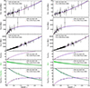 |
Fig. 1. OHD, GC, SN Ia, and BAO datasets with MCMC1 (left column) and MCMC2 (right) best-interpolating Bézier curves (blue curves) and 1–σ confidence bands for ℋ(z), 𝒟A(z), |

The best-fit values are listed in Table 4 and compared with the constraints on flat and non-flat ΛCDM models got from Planck TT, TE, EE + lowE + lensing data (Planck Collaboration VI 2020). In particular, in Fig. 1 the flat ΛCDM case is used as a benchmark for the best-fitting Bézier interpolations of OHD, GC, SN Ia, and BAO catalogs.
MCMC best fits.
Focusing on the cosmological parameters ωb, ωm, h0, and Ωk (see Table 4), we can deduce what follows below.
-
The MCMC1 analysis confirms and further refines the findings of Alfano et al. (2024b), which were based on SDSS data points though not in their final version presented by Alam et al. (2021).
-
The MCMC2 bounds tend to agree with the MCMC1 results, albeit with a) a smaller value of ωb and b) a barely consistent (at ≈1–σ CL) and positive Ωk.
-
In both analyses, the inclusion of the Pantheon+ catalog improves the constraints on Ωk, which are more compatible (within 1–σ CL) with the flat scenario or with small spatial curvature geometries.
-
Both MCMC1 and MCMC2 results are in agreement within 1–σ CL with the flat concordance model, though with larger attached errors.
-
For both analyses, the consistency with the non-flat extension of the ΛCDM (Planck Collaboration VI 2020) is at 2–σ CL, due to the estimate on h0.
-
The Hubble tension seems to be solved in favor of the Planck Collaboration VI (2020) value, h0 = 0.6736 ± 0.0054, consistent at 1–σ CL with both MCMC1 and MCMC2 estimates, whereas the value h0 = 0.7304 ± 0.0104 got from SNe Ia (Riess et al. 2022) is only consistent within 2–σ CL with MCMC1 and MCMC2 analyses.
-
In general, the best-fit values obtained from the MCMC2 analysis (performed using the DESI-BAO data) seems to be closer to the flat ΛCDM best-fits (Planck Collaboration VI 2020) than those from the MCMC1 procedure.
5. Reconstruction of the dark energy behavior
From the best-fit values of Table 4, we could now attempt the reconstruction of the DE behavior. We could use Ωk directly to model the curvature contribution and the combination of h0 and ωm to constrain the matter density parameter. Next, we used the CMB temperature, T0 = 2.7255 ± 0.0006 K, and the effective extra relativistic degrees of freedom, Neff = 2.99 ± 0.17 (Planck Collaboration VI 2020), to compute the radiation density parameter,  . Putting all these contributions together in a ΛCDM-like fashion, we defined the following function of the redshift:

At this point, we could single out the contribution of the DE density by subtracting Eq. (15) from ℋ2(z), obtained by squaring Eq. (1); namely,
where the coefficients βi in the last expressions and listed in Table 5 depend upon combinations of the coefficients αi and the cosmological parameters ωm, Ωk, and Ωr, reported in Appendix B.
DE reconstruction coefficients.
The reconstructed DE behaviors for both MCMC1 and MCMC2 analyses, obtained by inputting the best-fit values of Table 4 in Eq. (16), are portrayed in Fig. 2 and compared with the expectations for ΛCDM, ωCDM, and CPL models (Planck Collaboration VI 2020). The behavior from the MCMC1 analysis indicates a > 1–σ deviation from the cosmological constant paradigm at z ≲ 1.5, with a preference for a dynamical DE behavior that also differs (again, at > 1–σ CL) from the simplest models; that is, ωCDM and CPL.
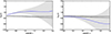 |
Fig. 2. Reconstructed DE behavior with z (blue curve) with attached confidence band (gray area), compared to the expected behaviors for the ΛCDM (filled circles), the wCDM (empty circles), and the CPL (empty squares) models. |
The MCMC2 analysis provides a reconstruction that, besides a small deviation at z ≲ 0.3, is always consistent (within 1–σ CL) with the ΛCDM, ωCDM, and CPL models. This indicates that the DE equation of state slowly evolves with z, mimicking the behavior of the cosmological constant at z ≳ 0.3 and deviating from it at smaller redshifts.
6. Final outlooks and perspectives
In this paper, we propose a strategy to separately measure baryons and CDM, by using different probes that may be classified in terms of low, intermediate, and early redshift points. Disentangling the matter sector, we infer DE at different stages of its evolution, resorting to a model-independent approach, based on the use of Bézier interpolation.
In this respect, we have extended the analysis performed in Alfano et al. (2024b) including the Pantheon+ catalog of SNe Ia, involving de facto all low- and intermediate-redshift probes, mentioned above.
Further, in view of the recent BAO data release by the DESI Collaboration (2024) – showcasing a ∼3–σ discrepancy at z ∼ 0.7 and claiming evidence for dynamical DE with respect to the SDSS results – we performed two separate MCMC analyses; namely,
-
MCMC1, involving SDSS data in conjunction with the other catalogs, and
-
MCMC2, replacing the SDSS dataset with the DESI release.
Thus, the use of Bézier parametric curves enables one to obtain model-independent bounds on h0, Ωk, ωb, and ωm, having been used, in particular, to:
-
(a)
infer an interpolated Hubble rate, ℋ(z), and estimate h0 through OHD,
-
(b)
evaluate an analytic expressions for the angular diameter distance, 𝒟A(z), of GCs, the luminosity distance,
 , of SNe Ia, and uncorrelated BAO observables, 𝒳, with no a priori assumptions on Ωk,
 -
(c)
break the degeneracy between ωb and ωm in the definition of rd with the interpolation of the correlated acoustic parameter, 𝒜(z).
With respect to Alfano et al. (2024b), the inclusion of the Pantheon+ catalog significantly improves the constraints on Ωk, further narrowing down the magnitude of a possible spatial curvature toward negligible values, and contributes to solving the Hubble tension in favor of CMB-consistent values; that is,  for MCMC1 and
  for MCMC2. Notably, the inclusion of SNe Ia disfavors the estimate h0 = 0.7304 ± 0.0104 based on local SNe Ia anchored to Cepheid stars (Riess et al. 2022).
In general, the cosmic bounds obtained from MCMC1 and MCMC2 (see Table 4 and Figs. A.1–A.2) are in great agreement (within 1–σ CL) with the flat ΛCDM model. In particular, albeit a slightly positive and small curvature, the MCMC2 analysis closely matches the expectations of the ΛCDM model (Planck Collaboration VI 2020), which is quite unexpected, since DESI-BAO findings seem to question the standard paradigm (DESI Collaboration 2024).
The corresponding results can therefore be summarized for the underlying analyses:
-
MCMC1, using SDSS-BAO data, highlights a deviation from the cosmological constant at z ≲ 1.5 and an overall agreement at larger redshifts.
-
MCMC2, using DESI-BAO data, exhibits a small deviation at z ≲ 0.3 and either an overall consistency (within 1–σ CL) with the ΛCDM paradigm or in line with a slowly evolving DE equation of state.
The latter result appears quite unexpectedly but in line with the above bounds on h0, Ωk, ωb, and ωm. Thus, the above improved cosmic bounds not only enable a better reconstruction of ℋ(z), but also the first attempt at a fully model-independent reconstruction of the DE evolution with z, based on the Bézier interpolation technique, which can be generalized in future works in terms of splines or alternatives to numerical reconstructions. Additionally, a further refinement in our model-independent procedure is mandatory, especially for the reconstruction and the modeling of DE equation of state, and therefore for the understanding of its nature. In this sense, besides improving all the hereby catalogs, it would be crucial for future works to:
-
resolve the discrepancy between DESI and SDSS datasets and get joint cosmic bounds;
-
work out model- and probe-independent calibration methods for gamma-ray bursts (Luongo & Muccino 2021b) and quasars (Risaliti & Lusso 2019), investigating and strengthening the constraints up to z ∼ 9.
Finally, the same procedure will be developed for additional DE scenarios to check the goodness of alternative models describing the cosmic speedup.
Acknowledgments
OL acknowledges Gianluca Castignani for fruitful debates on the topic of this work during his stay at the University of Camerino. MM is grateful for the hospitality of the University of Camerino during the period in which this work has been written and acknowledges Grant No. BR21881941 from the Science Committee of the Ministry of Science and Higher Education of the Republic of Kazakhstan. The authors are thankful to Anna Chiara Alfano for interesting discussions related to the subject of model-independent techniques.
References
- Abdalla, E., Abellán, G. F., Aboubrahim, A., et al. 2022, J. High Energy Astrophys., 34, 49 [NASA ADS] [CrossRef] [Google Scholar]
- Aizpuru, A., Arjona, R., & Nesseris, S. 2021, Phys. Rev. D, 104, 043521 [CrossRef] [Google Scholar]
- Alam, S., Aubert, M., Avila, S., et al. 2021, Phys. Rev. D, 103, 083533 [NASA ADS] [CrossRef] [Google Scholar]
- Alfano, A. C., Capozziello, S., Luongo, O., & Muccino, M. 2024a, J. High Energy Astrophys., 42, 178 [NASA ADS] [CrossRef] [Google Scholar]
- Alfano, A. C., Luongo, O., & Muccino, M. 2024b, A&A, 686, A30 [NASA ADS] [CrossRef] [EDP Sciences] [Google Scholar]
- Alfano, A. C., Luongo, O., & Muccino, M. 2024c, arXiv e-prints [arXiv:2408.02536] [Google Scholar]
- Amati, L., D’Agostino, R., Luongo, O., Muccino, M., & Tantalo, M. 2019, MNRAS, 486, L46 [CrossRef] [Google Scholar]
- Arjona, R., Cardona, W., & Nesseris, S. 2019, Phys. Rev. D, 99, 043516 [NASA ADS] [CrossRef] [Google Scholar]
- Aubourg, É., Bailey, S., Bautista, J. E., et al. 2015, Phys. Rev. D, 92, 123516 [Google Scholar]
- Bamba, K., Capozziello, S., Nojiri, S., & Odintsov, S. D. 2012, Ap&SS, 342, 155 [NASA ADS] [CrossRef] [Google Scholar]
- Belfiglio, A., Giambò, R., & Luongo, O. 2023, Class. Quant. Grav., 40, 105004 [NASA ADS] [CrossRef] [Google Scholar]
- Bernal, J. L., & Libanore, S. 2023, Cosmic Tensions– Lecture Notes (University of Cantabria) [Google Scholar]
- Beutler, F., Blake, C., Colless, M., et al. 2011, MNRAS, 416, 3017 [NASA ADS] [CrossRef] [Google Scholar]
- Blake, C., Brough, S., Colless, M., et al. 2012, MNRAS, 425, 405 [Google Scholar]
- Bonamente, M., Joy, M. K., LaRoque, S. J., et al. 2006, ApJ, 647, 25 [NASA ADS] [CrossRef] [Google Scholar]
- Borghi, N., Moresco, M., & Cimatti, A. 2022, ApJ, 928, L4 [NASA ADS] [CrossRef] [Google Scholar]
- Capozziello, S., De Laurentis, M., Luongo, O., & Ruggeri, A. 2013, Galaxies, 1, 216 [NASA ADS] [CrossRef] [Google Scholar]
- Carloni, Y., Luongo, O., & Muccino, M. 2024, arXiv e-prints [arXiv:2404.12068] [Google Scholar]
- Carlstrom, J. E., Holder, G. P., & Reese, E. D. 2002, Annual Rev. of Astron. Astrophys., 40, 643 [Google Scholar]
- Carroll, S. M. 2001, Liv. Rev. Relat., 4, 1 [NASA ADS] [CrossRef] [Google Scholar]
- Colgáin, E. Ó., Dainotti, M. G., Capozziello, S., et al. 2024, arXiv e-prints [arXiv:2404.08633] [Google Scholar]
- Conley, A., Guy, J., Sullivan, M., et al. 2011, ApJ Suppl. Ser., 192, 1 [CrossRef] [Google Scholar]
- Copeland, E. J., Sami, M., & Tsujikawa, S. 2006, Int. J. Mod. Phys. D, 15, 1753 [NASA ADS] [CrossRef] [Google Scholar]
- Cuceu, A., Farr, J., Lemos, P., & Font-Ribera, A. 2019, JCAP, 2019, 044 [Google Scholar]
- D’Agostino, R., Luongo, O., & Muccino, M. 2022, Class. Quant. Grav., 39, 195014 [CrossRef] [Google Scholar]
- De Filippis, E., Sereno, M., Bautz, M. W., & Longo, G. 2005, ApJ, 625, 108 [NASA ADS] [CrossRef] [Google Scholar]
- DESI Collaboration 2024, arXiv e-prints [arXiv:2404.03002] [Google Scholar]
- Di Valentino, E., Mena, O., Pan, S., et al. 2021, Class. Quant. Grav., 38, 153001 [NASA ADS] [CrossRef] [Google Scholar]
- Dunsby, P. K. S., & Luongo, O. 2016, Int. J. Geom. Methods Mod. Phys., 13, 1630002 [Google Scholar]
- Efstathiou, G. 2024, arXiv e-prints [arXiv:2408.07175] [Google Scholar]
- Efstathiou, G., & Bond, J. R. 1999, MNRAS, 304, 75 [NASA ADS] [CrossRef] [Google Scholar]
- Gialamas, I. D., Hütsi, G., Kannike, K., et al. 2024, arXiv e-prints [arXiv:2406.07533] [Google Scholar]
- Giarè, W., Najafi, M., Pan, S., Di Valentino, E., & Firouzjaee, J. T. 2024, JCAP, 2024, 035 [CrossRef] [Google Scholar]
- Glanville, A., Howlett, C., & Davis, T. M. 2021, MNRAS, 503, 3510 [NASA ADS] [CrossRef] [Google Scholar]
- Haridasu, B. S., Luković, V. V., Moresco, M., & Vittorio, N. 2018, JCAP, 2018, 015 [CrossRef] [Google Scholar]
- Hastings, W. K. 1970, Biometrika, 57, 97 [Google Scholar]
- Jiang, J.-Q., Giarè, W., Gariazzo, S., et al. 2024a, arXiv e-prints [arXiv:2407.18047] [Google Scholar]
- Jiang, J.-Q., Pedrotti, D., Santos da Costa, S., & Vagnozzi, S. 2024b, arXiv e-prints [arXiv:2408.02365] [Google Scholar]
- Jiao, K., Borghi, N., Moresco, M., & Zhang, T.-J. 2023, ApJ Suppl. Ser., 265, 48 [CrossRef] [Google Scholar]
- Jimenez, R., & Loeb, A. 2002, ApJ, 573, 37 [NASA ADS] [CrossRef] [Google Scholar]
- Luongo, O., & Muccino, M. 2018, Phys. Rev. D, 98, 103520 [CrossRef] [Google Scholar]
- Luongo, O., & Muccino, M. 2021a, MNRAS, 503, 4581 [NASA ADS] [CrossRef] [Google Scholar]
- Luongo, O., & Muccino, M. 2021b, Galaxies, 9, 77 [NASA ADS] [CrossRef] [Google Scholar]
- Luongo, O., & Muccino, M. 2023, MNRAS, 518, 2247 [Google Scholar]
- Luongo, O., & Muccino, M. 2024, A&A, 690, A40 [NASA ADS] [CrossRef] [EDP Sciences] [Google Scholar]
- Metropolis, N., Rosenbluth, A. W., Rosenbluth, M. N., Teller, A. H., & Teller, E. 1953, J. Chem. Phys., 21, 1087 [Google Scholar]
- Montiel, A., Cabrera, J. I., & Hidalgo, J. C. 2021, MNRAS, 501, 3515 [Google Scholar]
- Moresco, M. 2015, MNRAS, 450, L16 [NASA ADS] [CrossRef] [Google Scholar]
- Moresco, M., Cimatti, A., Jimenez, R., et al. 2012, JCAP, 2012, 006 [CrossRef] [Google Scholar]
- Moresco, M., Pozzetti, L., Cimatti, A., et al. 2016, JCAP, 2016, 014 [CrossRef] [Google Scholar]
- Moresco, M., Amati, L., Amendola, L., et al. 2022, Liv. Rev. Relat., 25, 6 [NASA ADS] [Google Scholar]
- Muccino, M., Luongo, O., & Jain, D. 2023, MNRAS, 523, 4938 [NASA ADS] [CrossRef] [Google Scholar]
- Peebles, P. J., & Ratra, B. 2003, Rev. Mod. Phys., 75, 559 [NASA ADS] [CrossRef] [Google Scholar]
- Perlmutter, S., Aldering, G., Goldhaber, G., et al. 1999, ApJ, 517, 565 [Google Scholar]
- Planck Collaboration VI. 2020, A&A, 641, A6 [NASA ADS] [CrossRef] [EDP Sciences] [Google Scholar]
- Ratsimbazafy, A. L., Loubser, S. I., Crawford, S. M., et al. 2017, MNRAS, 467, 3239 [NASA ADS] [CrossRef] [Google Scholar]
- Riess, A. G., Filippenko, A. V., Challis, P., et al. 1998, AJ, 116, 1009 [Google Scholar]
- Riess, A. G., Yuan, W., Macri, L. M., et al. 2022, ApJ, 934, L7 [NASA ADS] [CrossRef] [Google Scholar]
- Risaliti, G., & Lusso, E. 2019, Nat. Astron., 3, 272 [Google Scholar]
- Roy Choudhury, S., & Okumura, T. 2024, ApJ, 976, L11 [NASA ADS] [CrossRef] [Google Scholar]
- Schöneberg, N. 2024, JCAP, 2024, 006 [Google Scholar]
- Scolnic, D., Brout, D., Carr, A., et al. 2022, ApJ, 938, 113 [NASA ADS] [CrossRef] [Google Scholar]
- Shafieloo, A. 2007, MNRAS, 380, 1573 [CrossRef] [Google Scholar]
- Shafieloo, A., & Clarkson, C. 2010, Phys. Rev. D, 81, 083537 [NASA ADS] [CrossRef] [Google Scholar]
- Simon, J., Verde, L., & Jimenez, R. 2005, Phys. Rev. D, 71, 123001 [NASA ADS] [CrossRef] [Google Scholar]
- Stern, D., Jimenez, R., Verde, L., Kamionkowski, M., & Stanford, S. A. 2010, JCAP, 2010, 008 [Google Scholar]
- Sunyaev, R. A., & Zeldovich, Y. B. 1970, Comm. Astrophys. Space Phys., 2, 66 [Google Scholar]
- Sunyaev, R. A., & Zeldovich, Y. B. 1972, Comm. Astrophys. Space Phys., 4, 173 [Google Scholar]
- Tomasetti, E., Moresco, M., Borghi, N., et al. 2023, A&A, 679, A96 [NASA ADS] [CrossRef] [EDP Sciences] [Google Scholar]
- Vagnozzi, S. 2020, Phys. Rev. D, 102, 023518 [Google Scholar]
- Vagnozzi, S. 2023, Universe, 9, 393 [NASA ADS] [CrossRef] [Google Scholar]
- Wagner, J., & Meyer, S. 2019, MNRAS, 490, 1913 [NASA ADS] [CrossRef] [Google Scholar]
- Wang, D. 2024, arXiv e-prints [arXiv:2404.13833] [Google Scholar]
- Weinberg, S. 2008, Cosmology (Oxford, UK: Oxford University Press) [Google Scholar]
- Wolf, W. J., & Ferreira, P. G. 2023, Phys. Rev. D, 108, 103519 [NASA ADS] [CrossRef] [Google Scholar]
- Wolf, W. J., Ferreira, P. G., & García-García, C. 2024a, arXiv e-prints [arXiv:2409.17019] [Google Scholar]
- Wolf, W. J., García-García, C., Bartlett, D. J., & Ferreira, P. G. 2024b, Phys. Rev. D, 110, 083528 [CrossRef] [Google Scholar]
- Zhang, C., Zhang, H., Yuan, S., et al. 2014, Res. Astron. Astrophys., 14, 1221 [CrossRef] [Google Scholar]
Appendix A: MCMC1 and MCMC2 details
We used a modified version of the code from Arjona et al. (2019), which is based on the Metropolis-Hastings algorithm (Metropolis et al. 1953; Hastings 1970).
For each of the MCMC analyses run in this paper:
-
we worked out a preliminary MCMC analysis to obtain a test covariance matrix, and then
-
we performed the actual MCMC analysis to produce a single chain.
For both MCMC1 and MCMC2 chains the initial 100 steps have been removed as burn-in, leaving chains with overall lengths of N ∼ 1.3 × 10⁴. To asses their convergence we computed the corresponding autocorrelation functions at lag k
where ℒt is the value of the log-likelihood at the step t and  is the mean of the chain. From Eq. (A.1), we define the autocorrelation length l as the lag beyond which the autocorrelation function drops below the threshold ρl(ℒ) = 0.01. MCMC1 and MCM2 analyses provide small values l = {12, 13}, respectively, indicating that most of the samples in the chains are independent, as indicated by the effective sample size
giving high values ESS = {2178, 1967}, respectively.
The best-fit parameters got from MCMC1 and MCMC2 analyses are portrayed in the 1–σ and 2–σ contour plots of Figs. A.1–A.2.
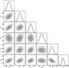 |
Fig. A.1. MCMC1 contour plots. Darker (lighter) areas display 1–σ (2–σ) confidence regions. |
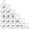 |
Fig. A.2. MCMC2 contour plots. Darker (lighter) areas dispaly 1–σ (2–σ) confidence regions. |
Appendix B: Coefficients of the dark energy reconstruction
We here show the explicit expressions of the coefficients βi used throughout the DE reconstruction reported in Eq. (16):
![$$ \begin{aligned} \beta _0 =&\,\frac{\left[\alpha _2+\alpha _0 \left(1+z_{\rm m}\right)^2-2 \alpha _1 \left(1+z_{\rm m}\right)\right]^2}{\alpha _0^2 z_{\rm m}^4}\,, \end{aligned} $$](/articles/aa/full_html/2025/01/aa52973-24/aa52973-24-eq52.gif)
![$$ \begin{aligned} \beta _1 =&-\frac{4\sqrt{\beta _0}\left[\alpha _2+\alpha _0 \left(1+z_{\rm m}\right)-\alpha _1 \left(2+z_{\rm m}\right)\right]}{\alpha _0 z_{\rm m}^2}\,, \end{aligned} $$](/articles/aa/full_html/2025/01/aa52973-24/aa52973-24-eq53.gif)

The errors σβi on the coefficients βi are computed using the covariance matrix  of each MCMC analysis and the partial derivative matrixes Jij = ∂βi/∂xj with variables xj = {α0, α1, α2, Ωk, ωm},
where σΩr is the error on the radiation density parameter, which is not correlated with the variables xj.
All Tables
All Figures
|
Fig. 1. OHD, GC, SN Ia, and BAO datasets with MCMC1 (left column) and MCMC2 (right) best-interpolating Bézier curves (blue curves) and 1–σ confidence bands for ℋ(z), 𝒟A(z), |
| In the text | |
|
Fig. 2. Reconstructed DE behavior with z (blue curve) with attached confidence band (gray area), compared to the expected behaviors for the ΛCDM (filled circles), the wCDM (empty circles), and the CPL (empty squares) models. |
| In the text | |
|
Fig. A.1. MCMC1 contour plots. Darker (lighter) areas display 1–σ (2–σ) confidence regions. |
| In the text | |
|
Fig. A.2. MCMC2 contour plots. Darker (lighter) areas dispaly 1–σ (2–σ) confidence regions. |
| In the text | |
Current usage metrics show cumulative count of Article Views (full-text article views including HTML views, PDF and ePub downloads, according to the available data) and Abstracts Views on Vision4Press platform.
Data correspond to usage on the plateform after 2015. The current usage metrics is available 48-96 hours after online publication and is updated daily on week days.
Initial download of the metrics may take a while.