| Issue |
A&A
Volume 695, March 2025
|
|
|---|---|---|
| Article Number | A20 | |
| Number of page(s) | 25 | |
| Section | Extragalactic astronomy | |
| DOI | https://doi.org/10.1051/0004-6361/202452570 | |
| Published online | 27 February 2025 | |
COSMOS-Web: Stellar mass assembly in relation to dark matter halos across 0.2 < z < 12 of cosmic history
1
Cosmic Dawn Center (DAWN), Denmark
2
Niels Bohr Institute, University of Copenhagen, Jagtvej 128, 2200 Copenhagen, Denmark
3
Aix Marseille Univ, CNRS, CNES, LAM, Marseille, France
4
The University of Texas at Austin, 2515 Speedway Blvd Stop C1400, Austin, TX 78712, USA
5
Laboratory for Multiwavelength Astrophysics, School of Physics and Astronomy, Rochester Institute of Technology, 84 Lomb Memorial Drive, Rochester, NY 14623, USA
6
Institut d’Astrophysique de Paris, UMR 7095, CNRS, Sorbonne Université, 98 bis boulevard Arago, F-75014 Paris, France
7
Space Telescope Science Institute, 3700 San Martin Drive, Baltimore, MD 21218, USA
8
Université de Strasbourg, CNRS, Observatoire astronomique de Strasbourg, UMR 7550, 67000 Strasbourg, France
9
Department of Physics and Astronomy, University of Hawaii, Hilo, 200 W Kawili St, Hilo, HI 96720, USA
10
Caltech/IPAC, 1200 E. California Blvd., Pasadena, CA 91125, USA
11
Department of Computer Science, Aalto University, P.O. Box 15400 FI-00076 Espoo, Finland
12
DTU Space, Technical University of Denmark, Elektrovej, Building 328, 2800 Kgs. Lyngby, Denmark
13
Center for Computational Astrophysics, Flatiron Institute, 162 Fifth Avenue, New York, NY 10010, USA
14
Institute of Physics, GalSpec, Ecole Polytechnique Federale de Lausanne, Observatoire de Sauverny, Chemin Pegasi 51, 1290 Versoix, Switzerland
15
NAF, Astronomical Observatory of Trieste, Via Tiepolo 11, 34131 Trieste, Italy
16
Instituto de Astrofísica de Canarias (IAC), La Laguna E-38205, Spain
17
Observatoire de Paris, LERMA, PSL University, 61 avenue de l’Observatoire, F-75014 Paris, France
18
Université Paris-Cité, 5 Rue Thomas Mann, 75014 Paris, France
19
Universidad de La Laguna, Avda. Astrofísico Fco. Sanchez, La Laguna, Tenerife, Spain
20
Department of Astrophysical Sciences, Princeton University, Princeton, NJ 08544, USA
21
NASA-Goddard Space Flight Center, Code 662, Greenbelt, MD 20771, USA
22
Purple Mountain Observatory, Chinese Academy of Sciences, 10 Yuanhua Road, Nanjing 210023, China
23
Centre for Extragalactic Astronomy, Durham University, South Road, Durham DH1 3LE, UK
24
Department of Physics, Northeastern University, 360 Huntington Avenue, Boston, MA 02115, USA
25
Department of Astronomy, University of Geneva, Chemin Pegasi 51, 1290 Versoix, Switzerland
26
Istituto Nazionale di Astrofisica (INAF), Osservatorio Astronomico di Padova, Vicolo dell’Osservatorio 5, 35122 Padova, Italy
27
Jet Propulsion Laboratory, California Institute of Technology, 4800 Oak Grove Drive, Pasadena, CA 91109, USA
28
Department of Physics and Astronomy, UCLA, PAB 430 Portola Plaza, Box 951547 Los Angeles, CA 90095-1547, USA
29
Department of Astronomy and Astrophysics, University of California, Santa Cruz, 1156 High Street, Santa Cruz, CA 95064, USA
30
Institute for Astronomy, University of Hawai’i at Manoa, 2680 Woodlawn Drive, Honolulu, HI 96822, USA
31
Sorbonne Université, Observatoire de Paris, PSL research university, CNRS, LERMA, 75014 Paris, France
32
European Southern Observatory, Karl-Schwarzschild-Str. 2, 85748 Garching, Germany
33
Department of Astronomy, University of Massachusetts, Amherst, MA 01003, USA
34
Astronomy Centre, University of Sussex, Falmer, Brighton BN1 9QH, UK
35
Institute of Space Sciences and Astronomy, University of Malta, Msida MSD 2080, Malta
⋆ Corresponding author; marko.shuntov@nbi.ku.dk
Received:
10
October
2024
Accepted:
17
January
2025
We study the stellar mass assembly of galaxies via the stellar mass function (SMF) and the coevolution with dark matter halos via abundance matching in the largest redshift range to date, 0.2 < z < 12. We used the 0.53 deg2 imaged by JWST from the COSMOS-Web survey, in combination with ancillary imaging in over 30 photometric bands, to select highly complete samples (down to log M⋆/M⊙ = 7.5 − 8.8) in 15 redshift bins. Our results show that the normalization of the SMF monotonically decreases from z = 0.2 to z = 12 with strong mass-dependent evolution. At z > 5, we find increased abundances of massive (log M⋆/M⊙ > 10.5) systems compared to predictions from semi-analytical models and hydrodynamical simulations. These findings challenge traditional galaxy formation models by implying integrated star formation efficiencies (SFEs) of ϵ ⋆ ≡M⋆ fb − 1 Mhalo−1 ≳ 0.5. We find a flattening of the SMF at the high-mass end that is better described by a double power law at z > 5.5, after correcting for the Eddington bias. At z ≲ 5.5, it transitions to a Schechter law, which coincides with the emergence of the first massive quiescent galaxies in the Universe, indicating that physical mechanisms that suppress galaxy growth start to take place at z ∼ 5.5 on a global scale. By integrating the SMF, we trace the cosmic stellar mass density and infer the star formation rate density, which at z > 7.5 agrees remarkably with recent JWST UV luminosity function-derived estimates. This agreement solidifies the emerging picture of rapid galaxy formation leading to increased abundances of bright and massive galaxies in the first ∼0.7 Gyr. However, at z ≲ 3.5, we find significant tension (∼0.3 dex) with the cosmic star formation (SF) history from instantaneous SF measures, the causes of which remain poorly understood. We infer the stellar-to-halo mass relation (SHMR) and the SFE from abundance matching out to z = 12, finding a non-monotonic evolution. The SFE has the characteristic strong dependence with mass in the range of 0.02 − 0.2, and mildly decreases at the low-mass end out to z ∼ 3.5. At z ∼ 3.5, there is an upturn and the SFE increases sharply from ∼0.1 to approach a high SFE of 0.8 − 1 by z ∼ 10 for log(Mh/M⊙)≈11.5, albeit with large uncertainties. Finally, we use the SHMR to track the SFE and stellar mass growth throughout the halo history and find that they do not grow at the same rate – from the earliest times up until z ∼ 3.5 the halo growth rate outpaces galaxy assembly, but at z > 3.5 halo growth stagnates and accumulated gas reservoirs keep the SF going and galaxies outpace halos.
Key words: galaxies: abundances / galaxies: evolution / galaxies: formation / galaxies: luminosity function / mass function
© The Authors 2025
 Open Access article, published by EDP Sciences, under the terms of the Creative Commons Attribution License (https://creativecommons.org/licenses/by/4.0), which permits unrestricted use, distribution, and reproduction in any medium, provided the original work is properly cited.
This article is published in open access under the Subscribe to Open model. Subscribe to A&A to support open access publication.
1. Introduction
The galaxy stellar mass function (SMF) is one of the most fundamental statistical measurements, quantifying the cosmic stellar mass assembly. It is shaped by all the physical processes that contribute to the growth of galaxies, and as such it reflects the cumulative history of star formation, mergers, and feedback processes. This is tightly linked to the dark matter halos in which galaxies form and evolve (White & Rees 1978). They provide the potential well in which gas can accrete and remain bounded, driving star formation. By studying the SMF, we can gain insights into the connection between galaxies and dark matter halos, which is essential for constraining theoretical models of galaxy formation and evolution.
Another importance in studying the SMF is that it quantifies the stellar mass density (SMD) assembled in the Universe at a given epoch. This, in turn, is a result of the integrated instantaneous cosmic star formation history (SFH) after correcting for stellar evolution processes (Madau et al. 1998). Comparisons between the SMD measured from SMF and the one obtained from integrating the cosmic SFH have shown a persistent discrepancy (e.g., Hopkins & Beacom 2006; Wilkins et al. 2008, 2019; Leja et al. 2015), with the integrated instantaneous SFH overpredicting the SMD. The reason for this tension remains poorly understood, and reconciling the two requires a detailed understanding of the various assumptions and systematics that enter the measurement of both quantities.
Historically, the SMF has been studied extensively in numerous works in the literature, from the very local Universe (e.g., Cole et al. 2001; Bell et al. 2003), across vast cosmic time intervals (e.g., Fontana et al. 2006; Pozzetti et al. 2007; Muzzin et al. 2013; Ilbert et al. 2013; Davidzon et al. 2017; Wright et al. 2018; McLeod et al. 2021; Weaver et al. 2023), to the earliest times that stellar masses could be robustly estimated (e.g., Grazian et al. 2015; Song et al. 2016; Bhatawdekar et al. 2019; Stefanon et al. 2021). These works rely on rest-frame optical photometric data either from ground-based imaging that is limited by resolution and sensitivity in the near-infrared (NIR), from the Hubble Space Telescope (HST) that is limited in wavelength coverage to < 1.6 μm, or from Spitzer that suffers from low resolution, source blending, and confusion in the IR. Furthermore, studies of the SMF in the early Universe (z > 6) have been carried out over very deep but small, pencil-beam surveys. These can be subject to significant cosmic variance relating to sampling over- and under-dense regions of large-scale structure (e.g., Steinhardt et al. 2021; Jespersen et al. 2024), and are unable to probe significant samples of some of the rarest and most massive galaxies at different epochs.
The launch of JWST has revolutionized our view of the early Universe with the unprecedented resolution and sensitivity at 1 − 5 μm from the Near Infrared Camera (NIRCam; Rieke et al. 2005). JWST observations confirmed that our z > 4 samples based on optical selection have been considerably incomplete in terms of typically red, dust-obscured, and massive (log M⋆/M⊙ > 10.5) systems (Barrufet et al. 2023; Gottumukkala et al. 2024; Weibel et al. 2024). Furthermore, early studies have revealed surprisingly high abundances of massive galaxies in the early Universe (Labbé et al. 2023; Xiao et al. 2024; Casey et al. 2024). These have challenged contemporary galaxy formation theories (Boylan-Kolchin 2023) by approaching the number density limit set by the dark matter halos and the universal baryonic reservoir.
Using JWST observations, several works have already investigated the SMF at z > 4 (Navarro-Carrera et al. 2023; Weibel et al. 2024; Harvey et al. 2025; Wang et al. 2024a) and agree on the enhanced abundances of massive (log M⋆/M⊙ > 10) systems at z > 6, compared to theory predictions. They have also revealed a significant contribution in the number density from sources hosting active galactic nuclei (AGNs), a subpopulation of which appear to be extremely red and compact (so-called little red dots (LRDs); Labbe et al. 2025; Greene et al. 2024; Matthee et al. 2024; Kokorev et al. 2024; Akins et al. 2024). These can boost the rest-frame optical flux and bias high the resulting stellar mass if the AGN component is not taken into account; therefore, they need to be carefully handled to avoid biases in the analysis. However, these works on the SMF are still limited to small areas and unable to probe the highest masses with high statistical significance.
The observed overabundance of massive galaxies can have important implications for baryon-to-star conversion efficiency in the early Universe, and thus on our galaxy formation models. Since this is related to the host dark matter halo, a systematic study of the relation between stellar and halo mass is necessary and still lacking in order to investigate the star formation efficiency (SFE) in a large redshift range and into the very early Universe. Several theories have been proposed to explain the overabundance of massive galaxies. For example, feedback-free bursts (FFBs; Torrey et al. 2017; Grudić et al. 2018; Dekel et al. 2023; Li et al. 2024; Renzini 2023), stochastic star formation (Pallottini & Ferrara 2023; Sun et al. 2023), and positive feedback from AGNs (Silk et al. 2024) in the early Universe can cause increased SFEs that can rapidly assemble high stellar masses. On the other hand, systematic biases and effects such as a nonuniversal initial mass function (IMF; e.g., Steinhardt et al. 2022) or outshining (e.g., Giménez-Arteaga et al. 2023; Narayanan et al. 2024) can lead to erroneously high or low inferred stellar masses, respectively. Furthermore, even modifications to the standard Λ cold dark matter (ΛCDM) cosmology have been suggested (Boylan-Kolchin 2023; Liu et al. 2024).
In this work, we use the largest JWST survey COSMOS-Web to consistently measure the SMF for the first time in 13.4 Gyr, or 97% of cosmic history. The NIRCam imaging at 1 − 5 μm allows us to compile highly complete rest-frame optical selected samples from z = 0.2 to z ∼ 10 (and rest-frame UV selected out to z = 12), and combined with 30 other photometric bands available in COSMOS spanning from the UV to the NIR, resulting in highly accurate photometric redshifts and stellar masses (Weaver et al. 2022). The large survey area (0.53 deg2) allows us to study the assembly of some of the most massive and rarest systems. The large volume probes a range of environments, and thus allows us to improve both the sampling statistics and the cosmic variance biases compared to previous work, especially at z ≳ 6. Using abundance matching, we also make the connection to dark matter halos and study the evolution of the integrated SFE out to z ∼ 12.
This paper is organized as follows. Section 2 presents the dataset we use to carry out our analysis, while Sect. 3 details the sample selection for our SMF measurements. In Sect. 4, we describe the methodology to measure the SMF, its associated sources of uncertainty, and the functional forms that we adopt to describe the SMF. The results are presented in Sect. 5 and compared with the literature. We discuss our results in Sect. 6 and put them into a broader perspective with respect to the cosmic stellar mass assembly and its connection to dark matter halos. Section 7 summarizes and concludes this work.
We adopt a standard ΛCDM cosmology with H0 = 70 km s−1 Mpc−1 and Ωm, 0 = 0.3, where Ωb, 0 = 0.04, ΩΛ, 0 = 0.7, and σ8 = 0.82. All magnitudes are expressed in the AB system (Oke & Gunn 1983). Stellar masses were obtained assuming a Chabrier (2003) IMF and, when comparing to the literature, stellar masses have been rescaled to match the IMF adopted in this paper.
2. Data
2.1. Space- and ground-based observations of COSMOS
This work relies on space- and ground-based multiband imaging data in the COSMOS field (Scoville et al. 2007). The cornerstone of our dataset is the multiband imaging from the JWST Cycle 1 program COSMOS-Web (Casey et al. 2023, GO#1727, PI: Casey & Kartaltepe), which we used to carry out the principal scientific analysis in this paper. Additionally, we relied on imaging in the COSMOS field from the deeper but smaller-area program PRIMER (Dunlop et al. 2021, GO#1837), mainly for validation purposes and completeness estimation.
COSMOS-Web is a photometric survey that consists of imaging in four NIRCam (F115W, F150W, F277W, F444W) filters and one MIRI (F770W) filter. The NIRCam (MIRI) filters reach a 5σ depth of AB mag 27.2 − 28.2 (25.7), measured in empty apertures of 0.15″ (0.3″) radius (Casey et al. 2023). Data reduction was carried out in the following way. For the January 2023 observational epoch we used version 1.8.3 of the JWST Calibration Pipeline (Bushouse et al. 2022), Calibration Reference Data System (CRDS) pmap-1017 and a NIRCam instrument mapping imap-0233. Subsequent data obtained in April 2023 were processed with an updated version of the JWST pipeline, version 1.10.0, alongside CRDS version 1075 (imap 0252). Finally, for data obtained in January 2024, we used the JWST pipeline 1.12.1 alongside CRDS version 1170 (imap 0273) for the version v0.6 and JWST pipeline 1.14.0 alongside CRDS version 1223 (imap 0285). Mosaics are created at 30 mas for the short wavelength and 60 mas for the long wavelength and MIRI filters. The NIRCam and MIRI image processing and mosaic making will be described in detail in Franco et al. (in prep.) and Santosh et al. (in prep.). This work uses the complete survey, imaged over three main epochs (January 2023, April 2023, January 2024), with missing visits (∼5%) completed in the April 2024 epoch.
We leveraged the wealth of legacy data in COSMOS by including the multiband imaging from ground- and space-based observatories, described in detail in Shuntov et al. (in prep.; see also Weaver et al. 2022). These data tightly sample the SED of galaxies from ultraviolet to mid-infrared wavelengths in over 30 photometric bands. The u band imaging comes from the CFHT Large Area U-band Deep Survey (CLAUDS; Sawicki et al. 2019) at a 5σ depth of 27.7 mag as measured from empty apertures of 2″ diameter size. For the optical data, we use The Hyper Suprime-Cam (HSC) Subaru Strategic Program (HSC-SSP; Aihara et al. 2018) DR3 (Aihara et al. 2022) in the ultra-deep HSC imaging region. This consists of five broad bands (g, r, i, z, y) and three narrow bands, with a sensitivity ranging 26.5–28.1 mag (5σ, 2″ aperture size). In addition, we include the reprocessed Subaru Suprime-Cam images with 12 medium bands in optical (Taniguchi et al. 2007, 2015). In the NIR, we also use the ground-based imaging from the UltraVISTA survey (McCracken et al. 2012; Dunlop et al. 2023) in four broad bands Y, J, H, Ks and one narrow band (1.18 μm, Milvang-Jensen et al. 2013). We use the latest and final UltraVISTA DR6, which provides homogeneous coverage over the entire field at the depth of the Ultra Deep stripes. Even though these ground-based data are at a lower resolution and sensitivity than NIRCam, they are complementary in terms of wavelength coverage. Crucially, the UltraVISTA bands fill in the wavelength gaps in the NIR left by the relatively sparse (4 band) JWST/NIRCam coverage. Finally, we also include the HST/ACS F814W band (Koekemoer et al. 2007) over the entire COSMOS area that is also covered by NIRCam.
2.2. Galaxy catalogs of photometry and physical parameters
To consistently measure photometry in ground– and space–based data that have very different resolutions, we used a model-fitting approach to extract source photometry in all 33 bands. We used SOURCEXTRACTOR++ (Kümmel et al. 2020; Bertin et al. 2020) to fit single Sérsic models convolved by the point spread function (PSF) in each band for all sources detected in a  combination (Szalay et al. 1999; Drlica-Wagner et al. 2018) of F115W, F150W, F277W, and F444W, PSF-matched to F444W. The structural parameters of the Sérsic models were fit on all NIRCam bands simultaneously, while the flux was fit for each band independently. The details of the photometry extraction and catalog making in COSMOS-Web are described in detail in Shuntov et al. (in prep.). We use the model-derived total photometry throughout the paper, unless stated otherwise.
We used the template-fitting code LEPHARE (Arnouts et al. 2002; Ilbert et al. 2006) to measure photometric redshifts and physical parameters on the 33 photometric bands spanning 0.3 − 8.0 μm. We fit a set of templates extracted from Bruzual & Charlot (2003) models that assume 12 different SFHs (exponentially declining and delayed), as described in Ilbert et al. (2015). For each SFH, it generates templates at 43 different ages going from 0.05 to 13.5 Gyr. Dust attenuation was implemented by varying the E(B − V) in the range of 0 − 1.2 from three attenuation curves (Calzetti et al. 2000; Arnouts et al. 2013; Salim et al. 2018) (we use dthe high-z analog curve from Salim et al. 2018). We added emission lines by adopting the recipe in Saito et al. (2020) and following Schaerer & de Barros (2009). We fit the normalization of the emission line fluxes by varying them by a factor of two (using the same ratio for all lines). Finally, the intergalactic medium absorption was accounted for by using the analytical correction of Madau (1995). LEPHARE provides the redshift likelihood distribution for each object, after a marginalization over the galaxy templates and the dust attenuation. We used it as the posterior redshift probability density function (PDF), assuming a flat prior. We adopted the median of the PDF(z) as our point estimate for the photometric redshifts. The physical parameters were derived in a second LEPHARE run. We used the same configuration as the one used to compute the photometric redshifts, except that we set the redshift to the point estimate previously established. We also associated a PDF with the mass by summing all the probabilities at a given mass by marginalizing over the templates and dust. These mass PDFs do not include the redshift uncertainties.
To calibrate LEPHARE and assess the photo-z performance (see Table 1), we used a sample of about 12 000 spectroscopic redshifts with a high (> 97%) confidence level out to z = 8. These are compiled from most spectroscopic programs in COSMOS (both public and private, e.g., Lilly et al. 2009; Kartaltepe et al. 2010, 2015; Silverman et al. 2015; Kashino et al. 2019; Le Fèvre et al. 2015; Casey et al. 2012; Capak et al. 2011; Kriek et al. 2015; Hasinger et al. 2018). The construction of the compilation, the individual surveys, and the properties and distribution of the galaxies will be presented in Khostovan et al. (in prep.).
Photo-z performance estimated using high-quality spectroscopic redshifts with > 97% confidence.
The stellar mass estimate can be significantly affected by SED modeling assumptions, such as the dust attenuation law and formation histories (e.g., Michałowski et al. 2012; Mitchell et al. 2013; Hayward & Smith 2015; Haskell et al. 2023, 2024; Pacifici et al. 2023). To investigate this in our data, we also ran CIGALE (Boquien et al. 2019) with a nonparametric SFH modeling and a different dust attenuation law. The CIGALE SED modeling and comparison with LEPHARE is described and discussed in more detail in Appendix F.
3. Sample selection
3.1. Selection function
The unprecedented combination of sensitivity and resolution in the NIR of NIRCam, coupled with wide and deep observations of COSMOS-Web allow us to compile complete galaxy samples in a large dynamic range of stellar mass. The deep imaging (∼28.0 mag in F444W) in the wavelength range ∼1 − 5 μm ensures that galaxies are detected in the rest-frame optical down to z ∼ 10. An advantage of the increase in depth in the NIR is that it leads to improved stellar mass completeness down to very low masses (see Sect. 3.2), and the detection of obscured and red populations, especially at the high-mass end that have likely been missed by previous studies (e.g., Weaver et al. 2023 for hints pre-JWST and e.g., Barrufet et al. 2023; Gottumukkala et al. 2024 for explanations using JWST). The NIR selection function at ∼1 − 5 μm can lead to some incompleteness of redshift ≲2 galaxies, especially those with young stellar populations and blue SEDs. However, these galaxies would have a low mass-to-light ratio and lie below our stellar mass completeness limits (Sect. 3.2) and therefore not bias our measurements.
The increased depth, coupled with the reduction of source blending thanks to the high resolution from space and the tight sampling of the SED by including ground-based bands, reduces photometric uncertainties and leads to more accurate estimates of physical parameters from SED fitting. The quality of the photo-z and physical parameters in our catalog is presented in detail in Shuntov et al. (in prep.). The photo-z show excellent performance, for different magnitude, color and type-selected samples, summarized in Table 1 with the standard metrics (σMAD, outlier fraction, bias). We inspected that the spec-z sample is reasonably well representative of the overall population, with no strong differences in the color or type selection functions. This allows us to select complete samples in 15 redshift bins from z = 0.2 to z = 12.
For the stellar mass estimates, we assessed their performance with respect to different SED modeling assumptions by comparing them with the CIGALE results (Appendix F). We find largely consistent results, albeit with a bias and scatter of about 0.1 − 0.3 dex toward higher masses by CIGALE.
We selected our sample over a total of ∼1926 arcmin2 (0.534 deg2). We applied bright star masks that are defined in the HSC images, which in our case are the same as in Weaver et al. (2022). These masks remove a conservatively large area around bright stars that contaminate the flux of nearby sources in the ground-based images. Even though the high-resolution NIRCam data is the pillar of our work and has a significantly smaller area affected by the bright stars, these conservative masks are necessary, since we include HSC and UltraVISTA fluxes in our SED fitting, and these data are unusable within the mask. These allow us to capture the Lyman break more accurately at z ≲ 5, especially in COSMOS-Web where HST coverage is limited, and more tightly sample the SED of galaxies especially in the NIR, where NIRCam coverage is limited to 4 bands, thanks to the UltraVISTA bands. Applying these masks results in an effective area of ∼1551 arcmin2, or 0.431 deg2.
We applied a cut in F444W magnitude that corresponds to ∼80% completeness (mF444W = 27.5; see Fig. 1 and Sect. 3.2). This ensures that the flux in the rest-frame optical is robustly measured at S/N > 5. Additionally, this cut also ensures that there is no spatial selection bias due to the small heterogeneity in depth in COSMOS-Web. This is rather conservative; however, the main goal of this work is leveraging the relatively large area to probe both ends of the typical “knee” of the Schechter form of the SMF, with a focus on the high-mass end. We also removed sources (0.13%) with poorly constrained photo-z that have > 75% of their P(z) outside the zphot ± Δz, where Δz is the width of the redshift bin. These are predominantly distributed near the low-mass completeness limit and their redshift distribution follows that of the full sample. The former was taken into account by the completeness correction (Sect. 3.2). Finally, we removed stars and brown dwarfs using the χstar2 of the star and brown dwarf SED templates fit by LEPHARE, coupled with compactness criteria.
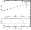 |
Fig. 1. Magnitude number counts in COSMOS-Web and PRIMER used for completeness estimation. Top: Total magnitude number counts as a function of F444W model magnitude in the COSMOS-Web and PRIMER-COSMOS catalogs. Bottom: Completeness fraction, defined as the ratio between the number counts of COSMOS-Web vs. PRIMER. |
3.2. Completeness limits
Quantifying the completeness of statistical samples is crucial for unbiased interpretations of the stellar mass assembly throughout cosmic time. The limited depth of the survey means that faint and typically low stellar mass galaxies start to be missed beyond a certain limiting magnitude (mlim), imposing a completeness limit in stellar mass, Mlim, which we quantify in this section.
We computed the stellar mass completeness at the low-mass end following the method of Pozzetti et al. (2010). Briefly, at each z bin, we took the 30% faintest galaxies as being the most representative of the population near the limiting stellar mass, and derived their mass (Mresc) by scaling the F444W magnitude to the magnitude limit of the survey (mlim):

Then, we defined the limiting stellar mass as the 95th percentile of the Mresc distribution. To compute the limiting magnitude, we relied on the F444W magnitude number counts. PRIMER-COSMOS is typically deeper than COSMOS-Web by about half a magnitude, and as such, PRIMER can serve us to estimate the magnitude limit of the COSMOS-Web catalog. The top panel of Fig. 1 shows the magnitude number counts in COSMOS-Web and PRIMER, along with a power law fit in the range 23 < mF444W < 27. We used model total magnitudes for both datasets, which is the reason why the number counts turn at brighter magnitudes than the image depth typically estimated from fixed-size apertures. The bottom panel shows the completeness fraction for COSMOS-Web defined as fcompl. = NCWeb/NPRIMER. We then defined the limiting magnitude, mlim, the magnitude at which fcompl. = 80%, which results in mlim = 27.5. We note that this was derived using the COSMOS-Web sample after applying the P(z) criterion, and therefore took into account any incompleteness introduced by this.
Using these limiting magnitudes in Eq. (1), we computed the mass completeness limits for each z bin. Fig. 2 shows the photo-z versus SMD histogram and the mass completeness limits for COSMOS-Web. We limited our analysis to samples more massive than these completeness limits.
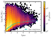 |
Fig. 2. Photo-z vs. stellar mass diagram showing the completeness limits for the COSMOS-Web catalog. The stellar mass completeness limits were derived by rescaling the stellar masses of the 30% faintest sources to the limiting magnitude of the survey (Eq. (1)) and taking the 95th percentile of this distribution. |
3.3. Removal of potential AGN contamination
Recent work from JWST has shown a high abundance of galaxies at 4 ≲ z ≲ 9 that exhibit active galactic nucleus (AGN) signatures identified from their broad Hα and/or Hβ lines (e.g., Kocevski et al. 2023; Maiolino et al. 2024; Fujimoto et al. 2023; Harikane et al. 2023a; Greene et al. 2024; Matthee et al. 2024). A fraction of these (∼20 − 30%) show extremely compact (i.e., point-like) morphologies and extremely red colors in the NIRCam long wavelength bands, and have therefore been dubbed LRDs (Matthee et al. 2024).
The origin of the red rest-frame optical continuum emission of LRDs is still not solved, and their photometric features can create important degeneracies during SED fitting. They can mimic strong Balmer breaks resulting in high stellar masses from aged stellar populations up to 2 dex, depending on the relative contribution of the stellar and AGN components (Wang et al. 2024b). Alternatively, they can also be fit by an SED with heavily dust-obscured components accounting for the rest frame optical emission, also resulting in high stellar mass. Therefore, unaccounted, these LRD can lead to biased measurements of high abundances of massive galaxies at high redshifts. LEPHARE, being the SED fitting code of choice for this work, does not fit a composite template of stellar and AGN components. Therefore, our stellar masses are prone to be biased for the AGN and LRD population.
We adopted a conservative approach of completely removing potential AGN and LRDs (in line with other recent works on massive, z > 4 galaxies, e.g., Chworowsky et al. 2024; Weibel et al. 2024; Harvey et al. 2025), by applying the following criteria at z > 3.5.
-
AGN-SED as the best fit. LEPHARE also fits AGN SEDs as part of the template set. However, this template does not distinguish the light originating from the stellar and AGN components and cannot estimate the stellar mass. We used the corresponding χAGN2 to identify sources whose photometry is best fit by a AGN SED, requiring that χAGN2 < χgal2.
-
Compact. We used the flux ratio in two different apertures (following Akins et al. 2024), and the effective radius Reff of the Sérsic fit for the compactness criterion:
 . We verify that the latter isolates clearly the locus of point-like sources, and the former corresponds to the FWHM of the F277W PSF. This is now possible in COSMOS-Web thanks to the high NIRCam resolution, compared to the lower resolution UltraVISTA bands of the previous COSMOS catalog iteration – COSMOS2020.
 -
Red. We use the two available NIRCam bands to identify the red colors of the LRD with the condition mF277W − mF444W > 1.5. This criterion is also described in detail in the systematical study of LRDs in COSMOS-Web by Akins et al. (2024). We individually inspected the stamps, photometry, and SED fits of many sources and verified that combining the three criteria efficiently identifies LRDs.
-
X-ray emission. We also identified sources with an X-ray counterpart by crossmatching within 1 arcsec with the Civano et al. (2016) catalog. We removed these regardless of whether or not they satisfied the previous three conditions.
The final condition to identify and remove sources dominated by AGN is: [(AGN-SED ∨ Red) ∧ Compact] ∨ X-ray. The main difference in our work is the inclusion of the AGN template criterion, whereas the (Red ∧ Compact) is an analogy of LRD condition from the literature (e.g., Labbe et al. 2025).
We note that these conditions still do not capture a potential AGN-dominated population that has both point-like and extended components and no X-ray counterparts, which can still introduce biases. Identifying and dealing with these would involve a 2D decomposition, which we leave for future work.
Finally, in Fig. B.1 we show the distribution of some of the properties of the AGN/LRD sample that we exclude from the analysis, and we discuss how they affect the SMF.
3.4. Summary of the selection criteria
Here, we summarize the criteria that we applied to select our samples in 15 redshift bins from z = 0.2 to z = 12.0.
-
mF444W < mlim, where mlim = 27.5.
-
Stellar mass selection above a completeness limit M⋆ > Mlim(z).
-
At P(z) > 25% within zphot ± Δz, where Δz is the width of the bin.
-
 , coupled with compactness criteria to remove stars and brown dwarfs.
 -
Does not satisfy the AGN/LRD criterion (AGN-SED ∨ Red) ∧ Compact, where AGN-SED: χAGN2 < χgal2, Compact:
 , Red: mF277W − mF444W > 1.5.
 -
No X-ray counterpart.
-
Outside of bright star masks defined in HSC.
-
Finally, we visually inspected sources of log(M⋆/M⊙) > 10.5 at z > 5, and removed possible artifacts.
Table 2 quantifies the number of sources remaining in our sample after applying the selection criteria.
Number of objects used in the analysis, after applying selection the criteria.
4. Measurements
4.1. 1/Vmax estimator for the SMF
We measured SMFs in each redshift bin using the 1/Vmax estimator (Schmidt 1968). This estimator essentially corrects the Malmquist (1922) bias, which refers to the fact that intrinsically faint galaxies can be observed within a smaller volume. With the 1/Vmax technique, each galaxy is weighted by the maximum volume in which it would be observed given the redshift range of the sample and magnitude limit of the survey. For the i-th galaxy, the Vmax, i is computed as
where Ωsurvey = 1520 arcmin2 and Ωsky = 41 253 deg2 are the surface area of the survey and the full sky, respectively, and dc(z) is the comoving distance at redshift z. The comoving volume Vmax was computed between zmin and zmax, where zmin is the lower redshift limit of the z bin and zmax = min(zbin, up, zlim), where zbin, up is the upper redshift limit of the z bin and zlim is the maximum redshift up to which a galaxy of a given magnitude can be observed given the magnitude limit of the survey mlim in F444W. Finally, the SMF was computed as
in the mass range starting from the mass completeness limit of each z bin, with a bin size of Δlog M = 0.25. Additionally, we corrected for the magnitude incompleteness by applying fcompl, i, which is the same completeness versus magnitude function as is presented in Sect. 3.2.
4.2. Sources of uncertainty
The SMF measurements are typically affected by three types of uncertainties of different origins, which need to be properly estimated. In the following, we describe how we account for these uncertainties in our measurements.
4.2.1. Poisson noise
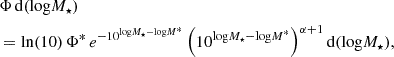
Since measuring the SMF is essentially counting galaxies in bins of stellar mass, it conforms to the Poisson counting statistic. Taking into account the 1/Vmax estimator, the Poisson uncertainty, σPois, was computed as  , where the sum runs over the number of galaxies in the bin. Fig. 3 shows the contribution of the different sources of uncertainties to the SMF as a function of stellar mass. The middle panel shows the Poisson uncertainties that become more important and dominant when the number counts are low; that is, at the high-mass end.
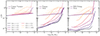 |
Fig. 3. Uncertainty budget of the SMF measurements. The three panels show the fractional uncertainty due to cosmic variance (left), Poisson (center), and SED fitting (right) in solid lines. The dashed lines, common to all panels, show the total uncertainty, obtained summing in quadrature the three contributions. For clarity, only a subset of our redshift bins are plotted. |
4.2.2. SED fitting uncertainties
Due to photometric errors and degeneracies in the SED fits, there are uncertainties in M⋆ and photo-z estimates that propagate to the SMF. We estimated the effects of stellar mass uncertainties from SED fitting on the SMF (σfit) by using the PDF(M⋆) computed by LEPHARE. We estimated σfit by drawing 1000 random samples from PDF(M⋆), computing Φ(M⋆) for each, and taking the standard deviation for each stellar mass bin. The right panel of Fig. 3 shows the relative uncertainty due to SED fitting, which is modest for low-mass galaxies but which becomes dominant at the high-mass end, mainly an effect of the Eddington bias.
We note that these uncertainties do not capture a wider range of plausible SFHs and other modeling assumptions than those we adopt for LEPHARE. In Appendix F we discuss how different SED modeling assumptions in CIGALE (such as nonparametric SFHs and dust attenuation) result in about 0.1 − 0.3 dex of scatter toward higher CIGALE masses. We do not propagate these uncertainties into our SMF measurements and caution that these should be considered as a lower limit.
Furthermore, uncertainties in the photo-z are also expected to have an impact on M⋆ and PDF(M⋆). However, these are expected to be relatively small and subdominant, given the high, percent-level, accuracy and sub-percent bias of our photo-z (Table 1). The effects of different sources of uncertainties in M⋆ and the SMF are examined in detail in the literature (e.g., Sect. 5 and Figs. 6–7 of Marchesini et al. 2009, Appendix A of Ilbert et al. 2013, Sect. 4 of Grazian et al. 2015, and Sect. 5.2 of Davidzon et al. 2017).
4.2.3. Cosmic variance
Since galaxies and halos are clustered, observing different fields implies a field-to-field variance in excess of Poisson noise, usually denominated cosmic variance (σcv, typically given as a fractional uncertainty; see Robertson 2010, Moster et al. 2011 for a definition). The final uncertainty is then σΦ2 = σPois2 + σfit2 + σcv2. Cosmic variance is naturally higher for smaller volumes/fields (Steinhardt et al. 2021; Vujeva et al. 2024), and also scales as a function of mass and redshift because galaxy bias scales as a function of mass and redshift (Moster et al. 2011). Although Moster et al. (2011) provided a cosmic variance calculator calibrated to observations, it was only calibrated in the low redshift regime and does not generalize to higher redshifts, where it provides significantly too high estimates of the cosmic variance, as discussed by Jespersen et al. (2024) and Weibel et al. (2024). Here we instead follow Jespersen et al. (2024) and recalibrate the cosmic variance to the UniverseMachine simulation suite (Behroozi et al. 2019). This directly incorporates the scatter in the stellar-to-halo mass relation (SHMR) ignored by Moster et al. (2011), which is on the order of 0.3 dex (Jespersen et al. 2022). To fit the cosmic variance, we first sample the number counts in the same angular size, redshift, and mass bins as used in this work, and then fit a power law in mass with a redshift-dependent normalization and slope. The fitting is done using scipy.optimize, incorporating the additional error terms identified by Jespersen et al. (2024). The results are shown in Fig. 3, and are significantly below what would be calculated with the Moster et al. (2011) calculator.
4.2.4. Eddington bias
The exponential cutoff of the SMF at M⋆ ≳ 1011 M⊙ means that uncertainties in the stellar mass will tend to upscatter more galaxies toward the more massive end than vice versa. This can inflate the number densities of high-mass galaxies, known as the Eddington bias (Eddington 1913). To account for the Eddington bias, we adopt the approach common in the literature (Ilbert et al. 2013; Davidzon et al. 2017; Weaver et al. 2022), where we infer the intrinsic SMF by fitting a functional form convolved with a kernel, 𝒟(M⋆), which describes the stellar mass uncertainty in bins of mass and redshift. Typically, this kernel takes the functional form of a product of Gaussian and Lorentzian components. However, in our work we build this kernel from the data itself for each redshift bin, by stacking the PDF(M⋆), centered at the median of the distribution, of all galaxies in the z bin. We verified that there is no appreciable change of the width 𝒟(M⋆) in different mass bins, which is the reason why we use a single kernel per z bin. The resulting 𝒟(M⋆) for all z bins are shown in Appendix A.
4.3. Functional forms to describe the SMF
The SMF is typically well described by a parametric function often referred to as the Schechter (1976) function. This function is a composite of a power law and an exponential cutoff function that describes the low- and high-mass ends, respectively. We consider three different functional forms to describe our measurements.
4.3.1. Single Schechter function
We fit our 1/Vmax measurements with the classical single Schechter function that is traditionally found to describe well the SMF at z > 2 (Ilbert et al. 2015; Grazian et al. 2015; Davidzon et al. 2017; Weaver et al. 2022). Written in terms of the logarithm of the stellar mass, it has the following form (Weigel et al. 2016):
where M* is the characteristic stellar mass that marks the so-called knee of the SMF separating the power law of slope α at the low-mass end and exponential cutoff at higher mass. Φ* sets the overall normalization that corresponds to the number density at M*.
4.3.2. Double Schechter function
For lower redshifts, however, numerous studies have shown that a double Schechter function better describes the galaxy number densities (e.g., Peng et al. 2010; Pozzetti et al. 2010; Baldry et al. 2012; Ilbert et al. 2013), given by the following form:
![$$ \begin{aligned}&\Phi \, {\mathrm{d}}(\mathrm{log}M_{\star }) = \mathrm{ln}(10) \, e^{-10^{\mathrm{log}M_{\star } - \mathrm{log}M^*}} \nonumber \\&\times \left[ \Phi ^*_1 \left(10^{\mathrm{log}M_{\star } - \mathrm{log} M^*}\right)^{\alpha _1+1} + \Phi ^*_2 \left(10^{\mathrm{log}M_{\star } - \mathrm{log} M^*}\right)^{\alpha _2+1} \right] {\mathrm{d}} ( \mathrm{log}M_{\star }). \end{aligned} $$](/articles/aa/full_html/2025/03/aa52570-24/aa52570-24-eq11.gif)
The two components share the same characteristic stellar mass, M*, but have different normalizations, Φ1* and Φ2*, and low-mass slopes, α1 and α2. In our work, we fit the double Schechter form out to z ∼ 3, finding that it provides a better fit to the observed SMF.
4.3.3. Double power law
We also considered a double power law (DPL) functional form to fit the SMF. The DPL has been increasingly used to describe the high-z measurements of the UV luminosity function (UVLF) (e.g., Bowler et al. 2014, 2020; Finkelstein & Bagley 2022; Finkelstein et al. 2024, and references therein). Since our measurements indicate that the high-z SMF also resembles a DPL (Figs. 4, 5), we carried out these fits and quantified how well this form describes the data. We adopted the following functional form of the DPL:
![$$ \begin{aligned} \Phi \, {\mathrm{d}}(\mathrm{log}M_{\star }) = \dfrac{\Phi ^*}{\left[10^{-(\mathrm{log}M_{\star } - \mathrm{log} M^*)({\alpha _1+1})} + 10^{-(\mathrm{log}M_{\star } - \mathrm{log} M^*)({\alpha _2+1})}\right]}, \end{aligned} $$](/articles/aa/full_html/2025/03/aa52570-24/aa52570-24-eq12.gif)
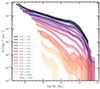 |
Fig. 4. Measurements of the SMF in COSMOS-Web in all 15 redshift bins. Each color corresponds to a different redshift bin. The solid lines mark the measurements, while the filled areas envelop the 1σ confidence interval including Poisson, cosmic variance, and SED-fitting errors. The SMF monotonically decreases at all redshifts, with a strong mass-dependent evolution. |
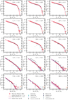 |
Fig. 5. Measurements of the SMF and its evolution with redshift in COSMOS-Web. Each panel shows the SMF in a given redshift bin, along with measurements in the literature from Weaver et al. (2022), Davidzon et al. (2017), Stefanon et al. (2021), Navarro-Carrera et al. (2023), Weibel et al. (2024), Harvey et al. (2025). The upper limits for empty bins are shown for the COSMOS-Web volume. In each z bin, we show the functional form that fits best the data (lowest Bayesian information criterion), while at z > 4.5, we show both the single Schechter and DPL fits for illustration. We plot the functions convolved with the Eddington bias kernel. |
where Φ* is the normalization at M*, which is the characteristic stellar mass that separates the two power law components described by the slopes, α1 and α2.
4.4. MCMC fits
To fit the functional forms of the SMF, we defined a Gaussian likelihood and employed the affine-invariant ensemble sampler implemented in the emcee code (Foreman-Mackey et al. 2013), using 6 × nparam walkers. To consider the chains converged, we used the autocorrelation time, τ, with the requirement that τ > 60 times the length of the chain and that the change in τ be less than 5%. We discarded the first 2 × max(τ) points of the chain as the burn-in phase and thinned the resulting chain by 0.5 × min(τ). We imposed flat priors on all parameters. For the double Schechter function fits, we required α1 < α2 and log(Φ2*/Φ1*) > 0. We let all parameters be fit at all z, except the low-mass slope at z > 5.5 that we set at α = −2 for both single Schechter and DPL. We discuss this choice in Sect. 5.4.
5. Results
5.1. Galaxy stellar mass function since z ∼ 10
Figures 4 and 5 present our measurements of the SMF in COSMOS-Web in each of the 15 redshift bins from z = 0.2 to z = 12.01. The low-mass cut is determined by the completeness limit estimated in Sect. 3.2, and the 1/Vmax is measured in bins of ΔM⋆ = 0.25 M⊙. The downward-pointing arrows in Fig. 5 represent the upper confidence limits of bins with zero galaxies, estimated as 1.841/V following Gehrels (1986), for the survey volume of COSMOS-Web.
Our work represents the most comprehensive set of measurements of the SMF in the largest redshift and stellar mass range to date. From Fig. 4, we can infer the evolution of the SMF since the first ∼360 Myr. As the redshift increases, the overall number densities of galaxies (the normalization of the SMF) decreases. The evolution has been slow since cosmic noon, with the normalization and shape staying very similar since z ∼ 2, only about 0.3 dex change in the last ∼10 Gyr. At earlier times, the evolution picks up pace and the normalization changes by 1.1–1.4 dex from z ∼ 6 to z ∼ 2. This is consistent with the known cosmic SFH (e.g., Madau & Dickinson 2014).
The evolution of the SMF with redshift can be interpreted in two extreme scenarios: pure mass evolution and pure density evolution (e.g., Johnston 2011; Ilbert et al. 2013). In the pure mass evolution scenario, galaxies grow in mass only by star formation, resulting in a horizontal shift of the SMF toward higher masses with decreasing redshift. Our results show that this evolutionary scenario is highly mass-dependent – a galaxy of M⋆ ∼ 109 M⊙ would increase by ∼0.9 dex between z ∼ 2.7 and z ∼ 0.3, while a M⋆ ∼ 1011 M⊙ would increase by ∼0.4 dex in the same time. This is consistent with the very efficient “mass quenching” of galaxies once they reach the same characteristic M* (Peng et al. 2010), which does not appear to evolve considerably with redshift (at least out to z ∼ 5, Sect. 5.4). In the pure density evolution scenario, the number density of galaxies increases due to the creation of new galaxies, resulting in a vertical shift. Our results show that this scenario too is highly mass-dependent – the low-mass end evolves faster than the high-mass end. However, the improved completeness at the low-mass end (by about 1 dex in M⋆) compared to previous work in COSMOS, reveals that the density evolution at masses just below the knee of the SMF is faster than the low-mass end, with ∼3 dex and ∼2 dex change in Φ since z ∼ 7 for log(M⋆/M⊙)∼10.4 and log(M⋆/M⊙)∼9, respectively. As the redshift increases, the low-mass slope steepens, and the knee flattens. The knee of the SMF, typically at log(M⋆/M⊙) > 10.5 seems to be disappearing at z > 3.5. Our measurements show that the number densities and their 1σ confidence intervals at the most massive end (beyond the knee) are within 1 dex since z = 5 and 2 dex at all robustly probed redshifts. However, due to the rarity of these massive galaxies, the limited survey volume, and possibly the effect of Eddington bias, the knee of the SMF and the most massive end becomes difficult to determine robustly at high-z. Nonetheless, the flattening of the high mass end at z > 5 indicates that a fraction of the most massive galaxies assembled very efficiently in the first few gigayears and have not grown significantly since, because of mass quenching.
In this work, we can also leverage the large MIRI coverage (∼0.2 deg2) and investigate the resulting SMF for sources covered at ∼7.7 μm. MIRI is important in probing the rest-frame optical at z > 4 and results in more robust stellar mass estimates (Wang et al. 2024a). In Fig. C1 we show the SMF in six z bins from z > 4.5 measured in the MIRI-covered area and compared with the one from the full COSMOS-Web. We find a very good consistency between the two, which also serves as a validation of our measurements in the full COSMOS-Web area. The small differences between the two remain within the uncertainties and small number statistics near the empty bin limits. This is somehow contrary to the conclusions in Wang et al. (2024a), but this remains sensitive to the various ingredients that go into the SED fitting and different codes used in the two works.
Finally, we also compare with the SMF measured from CIGALE, as is shown in Fig. F.2. This shows how different SED modeling assumptions propagate into the SMF and captures the variance and uncertainty arising from it. Overall, there is very good consistency between the two. However, the 0.1 − 0.3 dex higher masses by CIGALE result in enhanced abundances of more massive galaxies.
5.2. The 10 < z < 12 SMF
At 10 < z < 12, we carried out a more rigorous selection of galaxy candidates for our SMF measurement. In addition to the selection criteria outlined in Sect. 3, we required that P(z > 9) > 68%. Furthermore, we visually inspected the median HSC grizy stacks of each source and removed sources that show a counterpart, or are severely blended in this low-resolution image. This removed 25% of the initial selection, and resulted in 27 galaxy candidates at 10 < z < 12. We discuss their properties more in Sect. 6.4. We note that this conservative selection prioritizes purity, therefore the SMF measurement in this bin likely suffers from incompleteness. Another reason for the possible incompleteness is sources that have a photo-z solution at z < 3 but a secondary peak at z > 10, which even though they can be selected as z > 10 dropouts have a preferred SED solution at low redshifts. We do not investigate these further in this work, but they will be studied in detail in dedicated papers on the very high redshift population (e.g., Casey et al. 2024, Franco et al. 2024, Franco et al. in prep.).
By virtue of the large area of COSMOS-Web, this number of 27 objects that are brighter than AB mag 27.5 in F444W allows us to carry out a statistical measurement such as the SMF at 10 < z < 12. This results in an SMF that shows a power law decrease with a slope consistent with α ≈ 2 (see Sect. 5.4). We caution that this is only a tentative measurement, since at z > 10 the rest-frame optical is no longer probed by the F444W filter. In such cases, stellar mass estimates are highly prone to a number of systematic biases that arise from not probing the rest-frame optical. Additionally, other systematics can also be important at these redshifts, including a top-heavy IMF (Steinhardt et al. 2023). In the MIRI-covered area, ten sources have a MIRI F770W counterpart at S/N > 2, and the SMF for these sources remains consistent with the full area (Fig. C.1); however, the MIRI area remains insufficient to robustly measure the number densities, and does not significantly help to remove low-z outliers.
5.3. Comparison with the literature
Figure 5 also compares our measurement with a selection of recent results from the literature. We present comparisons with pre-JWST measurements from Weaver et al. (2022), Davidzon et al. (2017), Stefanon et al. (2021) and JWST measurements from Navarro-Carrera et al. (2023), Weibel et al. (2024), Harvey et al. (2025).
5.3.1. Comparison with previous measurements in COSMOS (pre-JWST)
In general, there is excellent agreement with previous measurements of the SMF in COSMOS by Davidzon et al. (2017) and Weaver et al. (2023) at all redshifts. The latter two rely on the ground-based UltraVISTA and the low-resolution, space-based, and relatively shallower (compared to NIRCam) Spitzer/IRAC data to sample the rest frame optical emission from z ≳ 2. Therefore, given this difference in data and photometry extraction techniques, the excellent agreement at z ≲ 2.5 attests to the robustness of the measurements. Thanks to the substantially deeper selection in the NIR from JWST, our work extends the z < 3.5 SMF down to ∼0.5 − 1 dex lower masses. However, there is some discrepancy, especially at the high-mass end between z ∼ 3 and z ∼ 5 with our results showing lower number densities compared to Weaver et al. (2023). By matching the samples in these z bins used in COSMOS2020 and in our catalog, we find that the dominant source of this difference is the M⋆ solutions in our COSMOS-Web catalog that are lower than those in COSMOS2020, especially at the high-mass end. This is likely due to the considerably improved depth and resolution from NIRCam which allows superior deblending and more accurate flux measurements. On the other hand, the M⋆ solution in COSMOS2020 is mostly constrained by the confusion-limited IRAC data, which can introduce uncertainties and biases in the flux measurements, resulting in biased M⋆ solutions toward higher values.
5.3.2. Comparison with the deepest HST and Spitzer measurements (pre-JWST)
Stefanon et al. (2021) measure the SMF from z ∼ 6 to z ∼ 10 using the deepest available data from HST and the Spitzer in the XDF/UDF, parallels and the five CANDELS (total of 731 arcmin2). Their measurements show higher number densities in the z ∼ 6 and z ∼ 7 bins by about 0.2 dex and 0.1 dex, respectively. The z ∼ 8 and z ∼ 9 bins are consistent with ours within the 1σ confidence intervals, albeit slightly lower at z ∼ 9. Their sample consists of exclusively Lyman-break galaxies, with H1.6 μm being the reddest detection band. Given the fact that in our work we are not limited to detecting only Lyman-break galaxies thanks to the 4.4 μm detection band (see e.g., Barrufet et al. 2023), the increased number densities of Stefanon et al. (2021) at z ∼ 6 − 7 is somehow surprising. The most likely reason for this difference might be cosmic variance due to the smaller volume. Indeed, spectroscopic redshift searches for overdensities in the GOODS fields (cornerstone of the Stefanon et al. 2021 study) have revealed several significant overdensities at z ∼ 6 − 7 (Helton et al. 2024), which can explain this difference in the SMF. Another potential reason is a difference in the redshift bin size and mean redshift of the sample, which we do not account for.
5.3.3. Comparison with JWST measurements
Several works have already reported measurements of the SMF leveraging the unprecedented sensitivity of JWST in the NIR. In one of the earliest works, Navarro-Carrera et al. (2023) measured the low-mass end of the SMF at 3.5 < z < 8.5 in the PRIMER-UDS and the HUDF fields, in a total of ∼20 arcmin2. Harvey et al. (2025), assembled some of the deepest JWST observations in numerous fields totaling 187 arcmin2 and measured the SMF at 6.5 < z < 13.5. Weibel et al. (2024), assembled the largest area (prior to our work) from JWST programs in the CANDELS-EGS, -COSMOS, -UDS and -GOODS-S fields, totaling 460 arcmin2 to study the SMF at z ∼ 4 − 9. All of these works probe the SMF down to lower masses by about 0.7–0.5 dex, thanks to the deeper observations compared to our work. However, our work probes more than three times the combined area of the former, and thus more robustly constrains the massive end of the SMF. In general, there is good agreement between the different JWST measurements.
In the z ∼ 6 and z ∼ 7 bins, the JWST results from Navarro-Carrera et al. (2023) show higher normalization of the SMF by about 0.5 dex. A likely explanation for this difference is cosmic variance, because there are the known overdensities in the GOODS-South field at these redshifts (Helton et al. 2024), which is a part of that measurement. Additional culprits might be uncertainties in the photometry and photometric calibration (given the relatively early release of that paper and the evolution of NIRCam calibration files since) and SED fitting systematics.
At z ∼ 8, z ∼ 9 and z ≳ 10, our measurements are consistent with those of Harvey et al. (2025), but ours show abundances of massive galaxies that are not probed by their ∼8 times smaller volume. At the low mass end, their measurements are consistent with extrapolating the SMF from our work beyond the completeness limit (at least at z < 10).
Compared to Weibel et al. (2024), our measurements are fully consistent at all redshifts. At z ∼ 9, our SMF is lower but within the 1σ uncertainties. This difference can be due to the small number statistics in the smaller field of Weibel et al. (2024) (54 galaxies at 8.5 < z < 9.5 compared to 209 in our sample at 8.5 < z < 10.0). Another likely contribution is the Δz = 0.5 difference in the redshift bins. However, at these redshifts all measurements should be interpreted cautiously because of the difficulty of measuring photo-zs and stellar masses with the wavelength coverage limited to ≲4.5 μm, especially with the limited NIRCam coverage of four bands in our work.
5.4. The best-fit model of the SMF
In this section, we present the fit functional forms of the 1/Vmax measurements of the SMF. The resulting best-fit functions represent the intrinsic SMF, with the effect of the Eddington bias removed. This is because during the fitting, we convolve the functions with the kernel describing the stellar mass uncertainties 𝒟(M⋆). We fit the double Schechter out to z = 3.5, single Schechter at z > 2.5, and DPL at z > 4.5, and used the Bayesian information criterion (BIC; Schwarz 1978) computed for the median posterior values to quantify the best-fitting functional forms. Table G.1 lists the median, 16th, and 84th percentiles of the Schechter and DPL parameters, along with the BIC for each fit. In the remainder of this paper, for a given z bin, we use the functional forms with lower BIC, unless stated otherwise. Figure 5 shows the fit functions and their 1σ confidence interval. The solid line and the shaded regions are obtained by computing the Schechter and DPL functions for 1000 randomly drawn samples of the posterior distribution and taking the median, 16th, and 84th percentiles. In this figure, we show the functions convolved with the Eddington bias kernel describing the stellar mass uncertainties 𝒟(M⋆) as they best match the data.
At z < 3.5, the data is better fit by a double Schechter function, which is a higher redshift than previous works that have done this out to z = 3.0 (e.g., Ilbert et al. 2013; Davidzon et al. 2017). This is likely because our improved depth, resolution, and wavelength coverage in the rest-frame optical compared to previous work allow us to 1) be more complete in detecting red quiescent and dusty systems and 2) more robustly determine the redshifts, stellar masses and SFR of this population at z > 3. An upcoming paper will investigate this in detail (Shuntov et al., in prep.). Since the double Schechter results from massive populations with suppressed SFR2 (Peng et al. 2010), this explains why we find it to be a better fit out to z = 3.5. Additionally, the effects of the Eddington bias can have significant effect on the shape of the SMF (e.g., Grazian et al. 2015; Davidzon et al. 2017), so a narrower mass uncertainty kernel (see Sect. 4.2) can result in revealing the double Schechter. The double Schechter out to higher redshifts can also be a result of probing a wider range of environments – Lovell et al. (2021) have shown in the FLARES simulation that a double Schechter describes the SMF at all redshifts and becomes increasingly pronounced for denser environments. However, given the fact that denser environments do indeed host more evolved galaxies with suppressed SFR, it is likely that the origin of the double Schechter form remains to be the rise of massive populations with lower SFR.
At 3.5 < z < 5.5, the best-fitting functional form is the single Schechter, and at z > 5.5 it is the DPL. However, both models are virtually indistinguishable visually, and quantitatively when integrating them to compute the SMD. Furthermore, at z ≳ 6 both models fail to robustly capture the high mass end at log(M⋆/M⊙) > 10.5. This is because of several reasons: mass uncertainties that can upscatter the measured number densities, but are not accounted for by the Eddington bias kernel; AGN component that can boost the flux but is unaccounted for in the SED fitting, and are not classified as AGN/LRD. We note that the majority of these sources with SED fitting solutions at z > 6 and log(M⋆/M⊙) > 10.5 are very difficult to constrain because they are red, highly dust attenuated and some have submillimeter counterparts; we discuss these further in Sect. 6.3.
5.5. Evolution of the model parameters with redshift
Figure 6 shows the evolution with redshift of the best-fit model parameters for the double/single Schechter and DPL fits, along with a compilation of literature results. At z > 5.5, we show the results from both the Schechter and DPL fits for illustration.
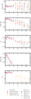 |
Fig. 6. Redshift evolution of the best-fit parameters for the Schechter (double and single) and DPL, along with a literature comparison. The different empty symbols correspond to the best-fit function adopted at a given redshift using the BIC. For illustration, at z > 5.5, we show the results from both Schechter and DPL fits. |
The characteristic mass log(M*/M⊙) is in the range of ≈10.6 − 11 and does not show a significant evolution out to z ∼ 4, in agreement with Weaver et al. (2023). However, the uncertainties are too large to infer an evolution meaningfully, and all the measurements in the literature are within the confidence intervals. This is because it is very difficult to constrain the log(M⋆/M⊙) > 10.5 regime at z > 6 with limited survey volumes, even with the 0.53 deg2 of COSMOS-Web. Constraints on this are poised to come from the next-generation Cosmic DAWN survey – 59 deg2 survey of the Euclid deep and auxiliary fields combining UV-IR data from Euclid, CFHT, HSC, and Spitzer (Euclid Collaboration 2025).
The normalization of the low-mass Schechter component, Φ1 (or Φ for the DPL), shows little evolution out to z ∼ 1, after which it decreases rapidly, in agreement with previous works (e.g., Weaver et al. 2023). The DPL results show an increased normalization compared to the Schecher component by ∼0.5 dex, but within the uncertainties. At z > 5, there is about 1 dex dispersion compared to the results from the literature (Weaver et al. 2023; Harvey et al. 2025; Weibel et al. 2024; Navarro-Carrera et al. 2023), but a general decreasing trend. The normalization of the high-mass double Schechter component, Φ2, decreases with redshift and shows relatively large uncertainties; compared to Weaver et al. (2023), the normalization is higher by about 0.3 dex, but the trend is in agreement.
The low-mass slope, α1 (or α for the single Schechter), remains roughly constant out to z ∼ 4, with a slight peak at z ∼ 1, in agreement with Davidzon et al. (2017), Weaver et al. (2023). At z > 4, the slope drops to ≈−2, and at z > 5.5, we set it to −2, because our data is not deep enough to constrain it. The choice of fixing α = −2 is motivated by the fact that literature results deep enough to provide meaningful constraints on α appear to converge at this value (Stefanon et al. 2021; Navarro-Carrera et al. 2023; Weibel et al. 2024; Harvey et al. 2025). Furthermore, extrapolating our measurements to lower masses with α = −2 is consistent with deeper measurements in the literature. We note that the low mass slope has an impact on the inferred SMD, which we quantify by sampling α1 out of a normal distribution with a variance of 50%. The low-mass slope of the high-mass component of the double Schechter function, α2, remains roughly constant, albeit with a slight increase, largely consistent with Weaver et al. (2023). Importantly, α2 − α1 remains consistent with unity out to z ∼ 3.5, confirming the predictions of the (Peng et al. 2010) phenomenological model. In Fig. 6, we also plot α2 of the high-mass end of the DPL component, although it has a different physical meaning. It has values of ≈−4, with large uncertainties that prevent us from identifying any significant redshift trend.
5.6. Cosmic evolution of the stellar mass density
The cosmic SMD describes the total stellar mass content in a volume of the Universe at a given epoch. Since the stellar mass growth in the Universe is directly related to the star formation activity, galaxy formation models need to link the observations of both consistently. Therefore, accurate measurements of SMD as a function of cosmic time are essential.
We derived the cosmic evolution of the SMD ρ⋆ by integrating our SMF presented in Sect. 5 in each redshift bin:
We used the best-fit models described in Sect. 4.3 by taking the models with the lower BIC (double Schechter at z < 3.5, single Schechter at 3.5 < z < 5.5 and DPL at z > 5.5). We took 108 M⊙ as the lower integration limit, which is the most commonly used in the literature, facilitating comparisons. At z > 2, our limiting mass is greater than 108 M⊙, so we relied on the extrapolations of the best-fit functions. The 1σ uncertainty was derived by integrating the 16th and 84th percentiles of the best-fit functions presented in Sect. 5.4.
The left panel of Fig. 7 shows the SMD from our work, along with a compilation of some recent measurements in the literature. Our results are shown in the solid orange line and the shaded region marking the 1σ confidence interval. Our measurements show a constant increase in ρ⋆ with cosmic time, with a flattening at z < 1, consistent with the peak and downturn of the cosmic SFH. At z > 1, ρ⋆ shows no significant change of slope within the uncertainties, at least out to z ∼ 9, indicating a steady buildup of the SMD with time.
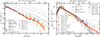 |
Fig. 7. Cosmic evolution of the stellar mass and star formation rate density. Left: Evolution of the SMD, showing a steady increase with time, with no significant change in slope at 1 < z < 9. Results from our work are shown in the orange line (median) and envelope (1σ uncertainty) in both panels. This is computed by integrating best-fit SMF at a given redshift from a common lower limit of 108 M⊙. The comparison with some of the most recent literature results includes Moutard et al. (2016), Wright et al. (2018), Bhatawdekar et al. (2019), Leja et al. (2020), Stefanon et al. (2021), Weaver et al. (2023), Navarro-Carrera et al. (2023), Weibel et al. (2024) and Harvey et al. (2025). The dashed green line shows the ρ⋆ obtained by integrating the Madau & Dickinson (2014) SFRD function multiplied by a time-dependent return fraction based on Chabrier IMF (see Sect. 5.6). The gray lines show the theoretical limits imposed by the HMF, scaled by the baryonic fraction fb and different integrated SFEs ϵ⋆, integrated from the same 108 M⊙ limit. Right: Inferred cosmic evolution of the SFRD. Comparison with the literature includes measurements of ρSFR from UVLF from Harikane et al. (2022, 2023b), Donnan et al. (2023, 2024), Willott et al. (2024), Pérez-González et al. (2023), Bouwens et al. (2023a) and Bouwens et al. (2023b) or from IRLF by Zavala et al. (2021), as well as the compilation in Madau & Dickinson (2014). All are obtained using a common lower integration limit of the UVLF of MUV = −17, including Bouwens et al. (2023a,b) that we rescale using a factor of 0.5 dex. All points are converted to a Chabrier IMF. The ρSFR inferred from SMF measurements is also shown for a compilation of the most recent literature works (Ilbert et al. 2013; Stefanon et al. 2021; Weibel et al. 2024; Harvey et al. 2025) shown only for the best-fit function, without confidence intervals for clarity. The solid lines turn to transparent at lower z that are not probed in the corresponding work. The solid (dashed) black line and shaded region show the true (observed) SFRD from Behroozi et al. (2019). Our results indicate lower inferred SFRD at z < 3.5, in tension with instantaneous SFR indicators, while at z > 7.5 we find remarkable consistency with recent JWST UVLF results. |
We compare our results with the literature, including Moutard et al. (2016), Wright et al. (2018), Leja et al. (2020), Bhatawdekar et al. (2019), Stefanon et al. (2021), Weaver et al. (2023), Navarro-Carrera et al. (2023), Weibel et al. (2024) and Harvey et al. (2025). Compared with the literature, generally, there is good agreement with our work, most notably with Weaver et al. (2023) at all redshifts. Compared to Weibel et al. (2024), there is a good agreement within the uncertainties at all redshifts, albeit with a ∼0.1 dex difference toward lower ρ⋆ from our measurements. Harvey et al. (2025) shows a steeper drop going from +0.5 dex at z ∼ 7 to −0.1 dex z ∼ 9, and flat trend to the z ∼ 11 bin. At the highest redshifts, the biggest difference is with the precipitous drop of the ρ⋆ by Stefanon et al. (2021); this can be because in the last two z bins they fix both log(M*/M⊙) = 9.5 (which is lower than values fit with our SMF) and α = −2. Leja et al. (2020) measure a higher ρ⋆ by about 0.1 dex, a difference that comes from their stellar masses being derived from nonparametric SFH modeling.
We also compare with the integrated SFRD function of Madau & Dickinson (2014), assuming a return fraction that depends on cosmic time fr(t − t′) = 0.048 log(1 + (t − t′)/0.88 Myr) (see Sect. 6.2 for justification), based on a Chabrier (2003) IMF, shown in the solid gray line. There is relatively good agreement in the general trend at z < 5, while at z > 5 our measurements are consistently lower with a slightly steeper slope. One reason for the discrepancy in this regime could be the fact that the SFRD by Madau & Dickinson (2014) at z > 5 is constrained with limited data from only two surveys (Bouwens et al. 2012a,b; Bowler et al. 2012) and is an extrapolation at higher redshifts. However, at all redshifts the Madau & Dickinson (2014) SFRD integration is constantly higher than the direct measurements from our work. This constant difference toward higher ρ⋆ obtained from integrating the SFRD compared to direct SMD measurements is persisting since the first comparisons between the two (e.g., Hopkins & Beacom 2006; Wilkins et al. 2008). Some of the reasons discussed in the literature to reconcile this discrepancy are overestimated instantaneous SFR measurements due to overestimated dust attenuation, uncertain UV luminosity to SFR conversion factor, which in turn can be due to an evolving IMF. We discuss this further in Sect. 6.2.
Finally, we also compare with the theoretical limits imposed by the dark matter halo evolution (Behroozi & Silk 2018). We scaled3 the halo mass function (HMF) (by Watson et al. 2013) with the universal baryonic fraction fb = 0.16 and with different values for the integrated SFE, ϵ⋆ = [0.05, 0.1, 0.3, 0.6, 1] and integrate it from the same 108 M⊙ mass limit. This comparison indicates relatively low cosmic SFEs below 5% at z > 1.5, with a trend toward increasing efficiencies at z ≲ 4 and z ≳ 7. This suggests that the assembly of halo and stellar mass has not happened at the same rate throughout cosmic history. This can be qualitatively explained by stagnating halo growth rate at z ≲ 5 and a gas reservoir that can keep the SFE increasing (Lilly et al. 2013). We study in closer detail ϵ⋆ and its evolution with both mass and redshift in Sect. 6.6, where we discuss this trend.
6. Discussion
6.1. Abundance of massive galaxies and transition from Schechter to a double power law
The form of the SMF and its evolution with redshift provide valuable constraints on physical models. The exponential cutoff of the Schechter function is thought to be a result of mass quenching (Peng et al. 2010), where AGN feedback in massive galaxies efficiently suppresses star formation and prevents the growth of more massive galaxies (Gabor & Davé 2015). The mass scale at which this happens is marked by the characteristic mass M* of the exponential cutoff. Therefore, robustly measuring the high-mass end of the SMF is important to shed light on the onset and efficiency of the AGN feedback in the early Universe.
Our results show a transition from the Schechter form to a DPL at z > 5.5. In the DPL, the SMF decreases following a power law with increasing mass, in contrast to the exponential cutoff of the Schechter. Although both functional forms do not fully fit the observed SMF points at log(M⋆/M⊙) > 10.5, the DPL providing a lower BIC also qualitatively confirms the observation of overabundance of massive galaxies at z ≳ 5. The existence of such massive galaxies in excess of predictions from a Schechter law suggests very efficient growth at early times. This is likely due to efficient cooling, gas accretion, and higher merger rates, which are shown to increase at earlier times (Duan et al. 2024). The transition to a Schechter law at z ≲ 5.5 also coincides with the rise of the first quiescent galaxies in the Universe (e.g., Carnall et al. 2023; Valentino et al. 2023). This indicates that the physical mechanisms that suppress galaxy growth start to take place at z ∼ 5.5 on a global scale, at least out to masses that we can probe in the COSMOS-Web volume. This is likely due to the onset of negative AGN feedback at these redshifts. However, we note that this remains only a tentative interpretation, since the relatively large uncertainties and potential systematics in photo-z and mass estimates at the high-mass, high-z end prevent us from drawing robust conclusions. Next-generation wide-area and deep NIR surveys from Euclid (e.g., Euclid Collaboration 2025) and Roman will be crucial in providing robust constrains on the evolution of the high mass end, log(M⋆/M⊙)≳10.2, at z > 5.
6.2. Implied cosmic star formation history
The total stellar mass assembled at a given epoch in a volume of the Universe is a result of the integrated star formation activity until that epoch, times a factor accounting for the stellar mass loss due to material returned to the ISM via stellar winds and supernovae (Renzini & Buzzoni 1986). Therefore, the SMD can be related to the star formation rate density (SFRD), ρSFR, as (Wilkins et al. 2008)
where fr is the stellar mass loss that depends on the age of the stellar populations, but also on metallicity.
The interest in comparing the implied SFH from SMD measurements to the one derived from star formation measurements is that a solid understanding of the physical processes that affect galaxy evolution will yield a consistent picture with both measurements in agreement. This is because both are affected by complementary systematic uncertainties. The SFRD is typically inferred from instantaneous indicators of star formation, such as rest-frame integrated UV emission, emission lines and IR luminosities, typically coming from young stellar populations (e.g., Kennicutt 1998; Calzetti et al. 2007; Madau & Dickinson 2014). These instantaneous indicators can be subject to greater uncertainty due to dust attenuation, and due to various assumptions in the stellar population synthesis models in deriving luminosity-to-SFR calibration factors. On the other hand, stellar masses are inferred from the light of more evolved stellar populations and are subject to different uncertainties (e.g., the assumed SFH in SED fitting). In this section we infer the cosmic SFH from our SMD measurements and compare to a range of literature results on the ρSFR, typically inferred from the instantaneous probe of SF – the UV luminosity function (UVLF).
We adopted a parametrized relation for the stellar mass loss that was calibrated using the computations in Dubois et al. (2024, Sect. 2.4 and Appendix A in their paper), and assuming a Chabrier (2003) IMF: fr(t − t′) = 0.048ln(1 + (t − t′)/0.88 Myr). We adopted a log-normal parametrization of ρSFR and fit our observed ρ⋆ using Eq. (8), finding
![$$ \begin{aligned} \rho _{\rm SFR}(z) = 0.05_{-0.01}^{+0.01}\, \mathrm{exp}\left[ -\dfrac{1}{2} \left(\dfrac{\mathrm{log}(1+z) - \mathrm{log}(1+1.95^{+0.17}_{-0.18})}{0.47_{-0.03}^{+0.03}} \right) \right]. \end{aligned} $$](/articles/aa/full_html/2025/03/aa52570-24/aa52570-24-eq15.gif)
The inferred ρSFR from ρ⋆ depends on the functional form assumed for the former. We also tested the parametrization of Madau & Dickinson (2014), Behroozi et al. (2013), as well as a double log-normal, but we found that Eq. (9) provides the best fit with lower χred2 and Bayesian information criterion.
The right panel of Fig. 7 shows the inferred cosmic SFH from our work (Eq. (9) with a solid orange line and a 1σ confidence interval). We show the SFH extrapolated to the highest redshifts probed by some of the work in the literature. The z > 12 part can be reasonably well constrained with this approach because after integration it has to result in the measured SMD at z < 12 from our work.
6.2.1. Comparison with the SFRD inferred from UVLF measurements
We compare the SFRD inferred from SMD measurements of our work to the one from instantaneous star formation measurements. These include the compilation from Madau & Dickinson (2014) out to z ∼ 7 using various tracers from UV to IR, Harikane et al. (2022, 2023b), Donnan et al. (2023, 2024), Willott et al. (2024), Pérez-González et al. (2023), Bouwens et al. (2023a,b) that are based on the UVLF, and Zavala et al. (2021) based on the IRLF. We rescale the results of Bouwens et al. (2023a,b) by a factor of 0.5 dex to bring them to a common lower integration limit of the UVLF MUV = −17. We also convert all measurements to a Chabrier IMF using a conversion factor of 0.63. We verify that the integration limits of MUV = −17 and M⋆ = 108 M⊙ are consistent for this comparison by using observed M⋆ − MUV relations (e.g., Song et al. 2016). We tested this further by reintegrating the SFRF by considering galaxies with M⋆ > 106 M⊙ and finding a negligible difference.
At z ≲ 3.5, we find that the SFRD inferred from our SMD is ∼0.3 dex lower than the SFRD from instantaneous SFR measurements by Madau & Dickinson (2014), with the largest difference around the peak of the cosmic SFH z ∼ 2. One reason for the lower SFRD inferred from the SMD can be in the assumed stellar mass loss function that has stronger effect at lower redshift (due to the integrated effect over time, Eq. (8)). We tested different mass loss functions (e.g, Conroy & Wechsler 2009; Ilbert et al. 2013) and found that although it can lower the difference and reconcile them z ≲ 1.5, it cannot fully account for the difference over a wider redshift range.
We compare our findings with Behroozi et al. (2019) UNIVERSEMACHINE model, which infers both the “true” and the “observed” SFRD (shown in solid and dashed black lines, respectively, in Fig. 7). The latter is obtained by applying correction that accounts for redshift-dependent observational systematic offsets. The true SFRD is consistently lower than the observed one, with the biggest difference (∼0.4 dex) around the peak of the SFRD (z ∼ 2). This is consistent with our results from the SMD, albeit with a difference of about 0.1 − 0.2 dex at z < 2.5. The observational systematic offset applied in Behroozi et al. (2019) is calibrated exactly against this tension between the integrated SFRD and the SMD, which has been repeatedly reported and studied in the literature (e.g, Hopkins & Beacom 2006; Wilkins et al. 2008, 2019; Leja et al. 2015). Our results corroborate this tension, the cause of which remains poorly understood, with several possible culprits (aside the stellar mass loss assumption). These include uncertain effects of dust attenuation on both stellar mass and SFR estimates, uncertain calibration for SFR indicators, IMF assumptions, and SFH and other modeling assumptions in SED fitting-derived stellar masses.
To shed some light on this tension, Wilkins et al. (2019) have investigated the effects of different (and more realistic) stellar population synthesis models on the luminosity-to-SFR calibration factors and on the resulting SFRD. They find that the recalibrated factors can lower the Madau & Dickinson (2014) SFRD by ∼0.2 dex. This would alleviate part of the tension that we report in our work, and is one likely explanation.
Furthermore, Leja et al. (2020) have found that nonparametric SFH modeling with PROSPECTOR can produce older stellar populations and higher stellar masses, resulting in higher ρ⋆ by up to a ∼50% compared to the literature. These measurements are shown in brown line in Fig. 7 (left) and are in good agreement with the Madau & Dickinson (2014) SFH. We also investigate the impact on nonparametric SFH modeled with CIGALE (Appendix F), which indeed yields ∼0.1 − 0.3 dex higher masses (Fig. F.1, Fig. F.2). We do not propagate these measurements to ρ⋆ but they are unlikely to fully account for the discrepancy. Nonetheless, older stellar populations from nonparametric SFH modeling is another likely explanation for this tension with the SFRD. Further investigation with a consistent dataset and methodology from both the SFR and stellar mass side, which is now possible with JWST, is necessary in order to reconcile the two fundamental cosmic observables.
At z > 7.5, the latest literature measurements from the UVLF, mostly from JWST data (Harikane et al. 2022, 2023b; Donnan et al. 2023, 2024; Willott et al. 2024; Pérez-González et al. 2023; Bouwens et al. 2023a,b), show a good agreement with the SFH inferred from our work, albeit with a large scatter and uncertainties. This remarkable agreement in the SFH from two parallel approaches solidifies the emerging picture of rapid galaxy formation leading to increased abundances of bright and massive galaxies very early in the Universe.
6.2.2. Comparison with the SFRD inferred from SMF measurements
We also infer ρSFR from some of the latest literature measurements of the ρ⋆ using the same procedure. These are shown in dashed, dotted, and dash-dotted lines from Weibel et al. (2024), Stefanon et al. (2021), Harvey et al. (2025). The lines turn to transparent at the lowest z range probed in the corresponding work. There are varying degrees of differences between these works, ours, and the ρSFR from instantaneous SF tracers, with none in very good agreement in a large redshift range at z > 6. This is mainly because these works do not measure the SMD at z ≲ 5, and the lower z measurements are essential in constraining the full z behavior. This is also shown by the result in Ilbert et al. (2013) that constrains the SFH from SMD measurements at 0.2 < z < 4.0, although in this case the lower maximum z limit likely creates the difference at z ≳ 3.
6.3. The most massive galaxies in COSMOS
In this work, we leverage the ∼4 × 10⁶ Mpc3 volume observed with COSMOS-Web to reveal some of the rarest and most massive objects in the Universe. Massive galaxies in the early Universe provide stringent constraints on the galaxy formation models and on the ΛCDM cosmology (Steinhardt et al. 2016; Behroozi & Silk 2018; Boylan-Kolchin 2023). A number of prior studies based on JWST have reported increased abundances of massive galaxies at z ≳ 5 (Labbé et al. 2023; Furtak et al. 2023; Xiao et al. 2024; Akins et al. 2023; Chworowsky et al. 2024; Casey et al. 2024) that have posed challenges to our models of galaxy formation and cosmology (Boylan-Kolchin 2023; Lovell et al. 2023).
We interpret the most massive galaxies observed in COSMOS-Web within the extreme value statistics (EVS; Lovell et al. 2023) formalism. EVS is a probabilistic approach to estimating the PDF(Mmax) of observing the most massive object at a given redshift and given cosmological volume. The EVS PDF(Mmax) is first derived for halos using theoretical HMFs, and the conversion to the PDF of the most massive galaxy is done using the universal baryon fraction fb, and stellar fraction f⋆. The latter is equivalent to the integrated SFE ϵ⋆ that we use in this work: M⋆ = Mh fb ϵ⋆. The stellar fraction is modeled as a lognormal distribution PDF(ϵ⋆) = lnN(μ = e−2, σ = 1), truncated between 0 and 1. This distribution is centered at 0.14 and incorporates the range of values found in the literature for ϵ⋆, as well as capturing a potential intrinsic scatter (e.g., Wechsler & Tinker 2018). However, it assumes no dependence on redshift and halo mass, the latter of which is well-known to exist, and the former is increasingly hinted at by recent studies.
Figure 8 shows the distribution of stellar masses and redshifts of our COSMOS-Web sample, along with the EVS confidence intervals for observing the most massive objects. We corrected the observed stellar masses for the effect of Eddington bias following Lovell et al. (2023)
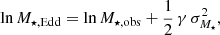
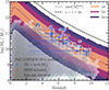 |
Fig. 8. Theoretical limits imposed from halo abundances of the most massive plausible galaxies at a given epoch and volume within the extreme value statistics (EVS) formalism. The colored regions indicate the EVS confidence intervals for the COSMOS-Web survey area of 0.43 deg2. The dotted line marks the median of the EVS distribution of the maximum plausible stellar mass, assuming a log-normal distribution of the SFE centered at ∼0.14, while the dashed line shows the 3σ upper limit assuming a SFE of unity. The grayscale hex bin histogram shows the M⋆ − zphot distribution of the full sample. Above the median |

where γ is the slope of the HMF at Mh = M⋆/fb, and σM⋆2 are the uncertainties on the stellar mass. This correction lowers the observed stellar mass because the slope is negative. The colored regions show the EVS 1σ, 2σ and 3σ confidence intervals that assume the lognormal distribution for ϵ⋆, while the dashed line shows the 3σ upper limit assuming ϵ⋆ = 1. Exceeding this limit would mean that there is more stellar mass than available baryons (under the assumption of a universal fb) and represents a 3σ tension with the underlying ΛCDM cosmology. Above the median  , we mark individual galaxies with points in Fig. 8.
None of the most extreme objects in our sample exceed the 3σ limit of ϵ⋆ = 1. However, a handful of objects approach the 3σ limit of the lognormal ϵ⋆ distribution centered at 0.14. In Fig. 8, we also mark the sources having MIRI photometry that in principle results in more robust stellar mass estimates (Wang et al. 2024a), but do not see a significantly preferred distribution in the M⋆ − z plane above the med line. In Fig. D.1 we show the F277W − F444W color versus F444W magnitude distribution of the extreme sample, color coded by E(B − V). A significant fraction (> 50%) of our extreme sample is very red (mF277W = mF444W > 1) and dust attenuated with E(B − V) > 0.5. The red colors and potentially high dust attenuation can make the derived photo-z and stellar masses uncertain due to degeneracies in the SED fitting. This is captured in Fig. 8 by the large redshift error bars of some of the candidates, making their nature uncertain.
We checked if our extreme sample, defined as  , have submillimeter counterparts by crossmatching with the SCUBA-2 selected sample of submillimeter galaxies (SMGs) by McKinney et al. (2024). This sample is one of the most comprehensive and up-to-date compilation that combines all archival photometric data from optical through radio in COSMOS. About 12% of our extreme sample are SMGs in the SCUBADive (McKinney et al. 2024) catalog. Given their extreme red colors (mF277W − mF444W > 1.2), these are highly dust attenuated and difficult cases to fit for our SED modeling that is configured to yield accurate results over all redshifts and populations (e.g., E(B − V) limited to 1.2). Indeed, SMGs are known to be difficult cases for SED fitting that, depending on modeling assumptions and available data, can have mass estimates varying up to 1 dex (Hainline et al. 2011; Michałowski et al. 2012). We find a relatively large scatter between our photo−z solutions and those by McKinney et al. (2024) that include FIR-to-radio data and more tailored SED modeling, which prefer lower redshift solutions by about Δz = 1 − 2. Figure D.1 shows that some of these sources are fit with low E(B − V) in our catalog, likely due to the dust attenuation-stellar mass degeneracy, and likely have overestimated stellar masses. We mark in yellow these sources in Fig. 8, and caution their interpretation.
We also crossmatched our extreme sample with spectroscopically confirmed SMGs and found two matches. One source has zspec = 5.051 from Jin et al. (2019), consistent with our  . This source has also been studied in Gentile et al. (2024) with the name ERD-1 and has a consistent stellar mass solution as ours (log(M⋆/M⊙) = 11.28). The second is found at
 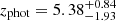 and log
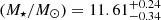 in our catalog, but has zspec = 3.68 and log(M⋆/M⊙) = 11.09 derived from spectroscopy (Liu et al. 2019). We do not exclude this source from our SMF which is in a M⋆ bin that has count one and is within the empty-bin confidence interval (Gehrels 1986, see also Sect. 5.1).
In Fig. D.2, we show one of the most extreme sources in our sample. The source ID = 762429 is found at 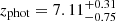 and log
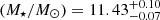 , with several modes in the P(z) down to z ∼ 3.5 as plausible solutions (with P(z < 5)≈5%). It has rising flux densities out to F770W and is highly dust attenuated. The system shows an extended morphology and possibly clumpy as indicated by the residual of the smooth Sérsic model. The rising flux densities can also be fit with the AGN template but resulting in overall worse χAGN2. However, from the clumpy morphology indicated by the residual images, it is possible that this is a merging system and therefore with components with significantly lower masses.
In summary, we find about 40 galaxies with masses that approach the 3σ limits imposed from halo abundances and local-Universe baryon-to-star conversion factors. These massive systems at high redshifts tend to be red and highly dust-attenuated, with 12% of them being detected at submillimeter and/or FIR. As such, they are very difficult cases for SED fitting and their photo-z and stellar mass solution are uncertain. These sources are certainly very interesting and warrant further in-depth investigation, since their extreme nature is a powerful probe of the galaxy formation theory. This would need to involve NIR spectroscopy and further submillimeter observations.
6.4. Galaxy candidates at 10 < z < 12
We selected 27 galaxy candidates at 10 < z < 12, as is described in Sect. 5.2; Fig. E.1 shows the distribution of some of their properties. Given the relatively shallow depth but distribution over a large area (0.53 deg2), these candidates are brighter than 27.5 AB mag and have a median of 26.7 AB mag in F444W. They have median F277W−F444W colors of ∼0.08 and are bluer than 0.4, with one candidate having mF277W − mF444W ∼ 0.7. Their median redshift is 10.3, and have 60% of their stacked P(z) at z > 10. Several candidates show a secondary peak at z ∼ 2.5 that has < 32% of the P(z < 9), while the stacked P(z) has 2.5% at z < 5. In this paper, we only analyze these candidates within the statistical context of the SMF (and quantities derived from it). We do not find that their number densities are in tension with limits from ΛCDM (see also Sect. 6.5 and Sect. 6.6), with the caution that they might suffer from incompleteness (cf. Sect. 5.2). However, these candidates are certainly interesting on their own, and warrant spectroscopic confirmation and in depth investigation.
Finally, we note that in Casey et al. (2024) we report nine exceptionally luminous and massive galaxy candidates at 10 ≲ z ≲ 12 in COSMOS-Web over half of the survey footprint of this paper (0.25 deg2). These were selected such that they have consistent zphot solutions with three different codes: LEPHARE, EAZY, and BAGPIPES, as well as with different photometry measurements (e.g., model fitting from SE++, aperture photometry). We find that only one source from our 10 < z < 12 sample is in common (source name COS-z10-4 in Casey et al. 2024). However, from the rest, all but one have broad and multimodal P(z) that encompasses a z > 9 solution. This difference is likely from the different LEPHARE configuration in this work, tuned to yield robust results for all redshifts and populations (e.g., high allowed attenuation and strong emission lines that can prefer a lower-z solution). Therefore, we take our results cautiously at z > 10 and the true redshift and nature of these candidates remains to be confirmed with spectroscopy.
6.5. Comparison to theoretical models
In this section, we compare to theoretical models and simulations to interpret some of the possible physical mechanisms behind our observations. Figure 9 compares the SMF from our work to a compilation of semi-analytical (ASTRAEUS, Hutter et al. 2021; Cueto et al. 2024; SANTA CRUZ SAM, Yung et al. 2019; DREAM, Drakos et al. 2022; GAEA De Lucia et al. 2024), hydrodynamical simulations (BLUETIDES, Feng et al. 2016; Wilkins et al. 2017; FLARES, Lovell et al. 2021; Vijayan et al. 2022; Wilkins et al. 2023; TNG100, Springel et al. 2018; Nelson et al. 2018; Pillepich et al. 2018; Marinacci et al. 2018; Naiman et al. 2018), the analytical feedback-free starbursts (FFB) (Dekel et al. 2023; Li et al. 2024), and the early dark energy (EDE) model (Liu et al. 2024). For brevity, we focus only on the SMF at z > 5. We show our measurements of the SMF in the orange circles and the 1σ confidence region of the fit parametric forms. The latter take into account the Eddington bias and therefore represent a more just comparison to the simulations. We note that for this compilation, we compare the SMFs at the median redshift that falls in the redshift bins from our work. This neglects potential differences in the redshift distributions. We note this caveat and do not attempt to correct for it.
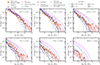 |
Fig. 9. Comparison of the COSMOS-Web SMF to theoretical models. Measurements and best fits from this work are shown in the orange circles and filled region. We compare with the predictions from the FFB model by Dekel et al. (2023), Li et al. (2024), which are based of UNIVERSEMACHINE (Behroozi et al. 2019) corresponding to different maximum SFEs (ϵ⋆) in the FFB regime, shown with the solid lines. We also show the SMF from a number of semi-analytical (ASTRAEUS, Hutter et al. 2021; Cueto et al. 2024; SANTA CRUZ SAM, Yung et al. 2019; DREAM, Drakos et al. 2022; GAEA De Lucia et al. 2024) and hydrodynamical simulations (BLUETIDES, Feng et al. 2016; Wilkins et al. 2017; FLARES, Lovell et al. 2021; Vijayan et al. 2022; Wilkins et al. 2023; TNG100, Springel et al. 2018; Nelson et al. 2018; Pillepich et al. 2018; Marinacci et al. 2018; Naiman et al. 2018), and the predictions of the Early Dark Energy model by Liu et al. (2024). |
6.5.1. Comparison with simulations
In Fig. 9, we make a comparison with an inexhaustive list of semi-analytical and hydrodynamical simulations. Overall, there is a relatively good agreement between SMFs from our work and the simulations, especially out to z ∼ 7. At z > 7.5 our measurements are consistently above the simulations. The best agreement out to the highest z ∼ 11 is with the FLARES simulation (Lovell et al. 2021; Vijayan et al. 2022; Wilkins et al. 2023). This is perhaps unsurprising because FLARES consists of a suite of zoom-in hydrodynamical simulations within larger cosmological volumes to study rare, massive structures at z > 5. The fact that FLARES probes the widest range of environments, from extremely underdense voids, to the most overdense high redshift structures, can explain their higher SMF and the closest agreement to ours. Lovell et al. (2021) show a strong dependence of the SMF on the environment and suggest that the higher SMF compared to other observations and simulations at M⋆ ≳ 1010 M⊙ is due to small volume probed by the latter, which does not probe extreme environments that can have a strong impact on the SMF.
The ASTRAEUS semi-analytical model (Hutter et al. 2021) provides an insight into how the IMF assumption impacts the resulting SMF. Cueto et al. (2024) computed the SMF using both a universal IMF and one that evolves toward an increasingly top-heavy IMF at higher redshifts. This results in lower mass-to-light ratios and a slower buildup of stellar mass, as shown by the ∼1 dex lower SMF for the evolving IMF compared to the universal IMF (solid and dashed yellow lines in Fig. 9). In our work, we assume a universal Chabrier (2003) IMF, so applying an evolving top-heavy IMF would result in lower stellar masses and number densities. However, the SMF from ASTRAEUS shows steeper slopes and increased number densities at the low-mass at all redshifts.
One aspect that these comparisons with simulations highlight is the overabundance of massive galaxies, especially at z ≳ 7, measured in our work, but also in recent work from JWST (e.g., Weibel et al. 2024, cf. Sect. 6.3). The surprising abundances of such systems stretch our current theories of galaxy formation and potentially the ΛCDM model. As a consequence, they can be powerful probes of our theory. In the following, we discuss possible scenarios that can explain these observations.
6.5.2. Possible physical mechanisms that can produce an overabundance of massive galaxies
The FFB model by Dekel et al. (2023), Li et al. (2024) postulates that at early times, the most massive dark matter halos can have a very high SFE (∼100%) due to starbursts that are free of feedback. These feedback-free bursts can happen in dense star-forming clouds (∼3 × 103 cm−3), when the free fall time is ≲1 Myr, shorter than the time for massive stars to develop winds and supernovae feedback (Torrey et al. 2017; Grudić et al. 2018). The bursts can last a few million years and reoccur during a phase of about 100 Myr. The FFB regime is activated above a halo mass threshold, dependent on the redshift ![$ M_{\mathrm{h}}^{\mathrm{FFB}} \sim 10^{10.8} \, [(1+z)/10]^{-6.2} $](/articles/aa/full_html/2025/03/aa52570-24/aa52570-24-eq26.gif) (Dekel et al. 2023), in which the SFE reaches a maximum
(Dekel et al. 2023), in which the SFE reaches a maximum  . In the Li et al. (2024) implementation of the FFB, the mean SFR of a galaxy in the FFB regime is modulated by the maximum SFE:
  , where Ṁh is the halo growth rate. Then stellar masses (and consequently SMF) are obtained by adding the time-integrated SFR contribution from the FFB mode on top of the nominal SFR based on the Behroozi et al. (2019) UNIVERSEMACHINE empirical model (see Li et al. 2024, for details). In Fig. 9 we show the predictions from the FFB model for different
  , including the no FFB regime of
  , which is essentially the UNIVERSEMACHINE model. Out to z ∼ 7 our results agree with the no FFB regime; while at higher redshifts our SMF would be consistent with an evolving
  of ∼0.1 at z ∼ 8 to ∼0.2 − 0.5 at z > 8.5. Additionally, our measurements also suggest a possible mass dependence of the
  – the most massive end of our SMF moves toward higher FFB efficiencies. This is not excluded by the FFB model, since the halo mass is a key ingredient and the
  can, in principle, depend on mass. Therefore, these observations can serve to properly tune the parameters of the FFB model, something that we do not attempt and leave for future work. However, given the uncertainties in the SMF (and M⋆) at these redshifts, it is difficult to provide robust constraints from such photometric surveys alone.
Stochastic bursts of star formation in the early phases of high-z galaxies can produce rapid stellar mass growth. These bursts can happen on a scale of about 5 Myr and can reoccur in a time span of about 100 Myr, leading to an increased integrated SFE (ϵ⋆), qualitatively consistent with our observations of the SMF. This hypothesis has been studied theoretically Pallottini & Ferrara (2023), and is found to explain the observed abundances of bright galaxies at z > 10 (Shen et al. 2023; Sun et al. 2023). The stochastic and bursty SFH is also consistent with the FFB model (Dekel et al. 2023; Li et al. 2024). The transition to stochastic star formation around z = 9 has also been identified observationally by Ciesla et al. (2024), showing that at z > 9 there is evidence for about 87% of massive galaxies having had stochastic star formation in the last 100 Myr.
Bursty SFHs can produce a scatter in galaxy UV luminosities at a given halo mass, leading to a dispersion in the MUV − Mh relation that is found to increase with decreasing halo mass (Sun et al. 2023). According to this model, the MUV − Mh scatter can reproduce increased abundances of luminous galaxies without the need of enhanced SFEs. Gelli et al. (2024) implement such a model and find that it can successfully match the observations of the UVLF and ρSFR up to z ∼ 12, using a constant SFE, while it still falls short at z ∼ 14. Their prediction on the ρSFR is shown in the purple curve in Fig. 7. However, this model remains to be extended to stellar masses and compared against SMF. Clustering analysis in COSMOS-Web by Paquereau et al. (2025) measures galaxy bias that tends to disfavor a scenario with high shochasticity and scatter.
Positive feedback from supermassive black hole (SMBH)-driven AGNs in the very early Universe can considerably increase the SFE, as is argued by Silk et al. (2024). In this hypothesis, star-forming galaxies at z ∼ 10 can host an AGN that enhances gas accretion onto both star-forming regions and the central SMBH. This, in turn, causes momentum-conserving AGN outflows and radiatively cooled turbulence, which, coupled with efficient cooling of the shocked gas due to the ultracompact galaxy, leads to a dense and cool phase with increased star formation. This positive feedback from AGN causes the first episodes of vigorous star formation at z ≳ 10, which then transitions to negative feedback and quenching due to gas depletion by energy-conserving AGN outflows at z ≲ 6. The positive feedback phase could be active in compact galaxies that have their central AGN obscured (Silk et al. 2024). Therefore, this scenario is also consistently linked to the emerging abundant population of compact AGN-dominated sources at z > 5 with massive (107 − 109 M⊙) black holes (Labbe et al. 2025; Greene et al. 2024; Matthee et al. 2024; Kokorev et al. 2024).
Qualitatively, our measurements are consistent with the positive feedback scenario. The transition from the Schecter function to the DPL, as well as the monotonic increase with mass of the integrated SFE close to 100% (discussed in Sect. 6.6) at z ∼ 6, all coincide with the transition from negative to positive AGN feedback. However, adequate data to constrain the parameters of this unified theory of the coevolution of SMBH and galaxies is still lacking, and details on how the positive feedback scenario would reflect on galaxy and AGN abundances (the former being the scope of this paper) are not yet developed. One way to detect the hidden momentum-driven positive AGN feedback according to Silk et al. (2024) is indirectly by searching for very high specific star formation rates. This would require follow-up spectroscopy of the most massive high-z candidates in this work.
Modifications of the ΛCDM cosmology are another alternative explanation. One proponent is the EDE model that can produce higher abundance of massive halos (Klypin et al. 2021). This excess number of massive halos can host galaxies assembled with a more modest ϵ⋆ than the higher one implied by our measurements within the standard cosmology. This can explain the observed abundance of massive galaxies without considerable modification to the galaxy physics that regulates the SFE. Liu et al. (2024) have studied the implications of the EDE model on the SMF, showing that it indeed predicts increased abundances. These predictions are shown in the gray lines and square symbols in Fig. 9. This model largely overpredicts the SMF out to z ∼ 9 but agrees at z > 10. However, in their application, Liu et al. (2024) assume a SHMR calibrated on pre-JWST data (by Stefanon et al. 2021, obtained from abundance matching), which as we show in the next section can be very uncertain (see also Shuntov et al. 2022). Accurately constraining the SHMR requires the implementation of halo occupation distribution (HOD) models that need to predict both galaxy abundance and clustering. Therefore, coupling clustering measurements to the abundances is necessary to provide more meaningful constraints on the EDE model.
6.6. Connection to dark matter halos and the inferred star formation efficiency
In this section, we use the SMF measurements to explore the connection between galaxies and dark matter. Galaxies grow in dark matter halos through star formation by converting the available baryonic gas, given by the cosmic baryon fraction fb ≈ 0.16, and through merging. This results in a relation between the stellar and the halo mass M⋆ = ϵ⋆ fb Mh, referred to as the SHMR (see Wechsler & Tinker 2018, for a review). Correspondingly, this establishes a relation between the cumulative number densities of galaxies and halos  (Behroozi & Silk 2018). ϵ⋆ is the SFE integrated over the lifetime of the halo4. In this paper, we provide some of the first systematic quantification of the integrated SFE from JWST, down to the earliest ages of the Universe. Additionally, a study by Paquereau et al. (2025) provides complementary constraints from HOD modeling of galaxy clustering in COSMOS-Web.
We inferred the SHMR by carrying out nonparametric abundance matching (AM; Marinoni & Hudson 2002; Kravtsov et al. 2004; Vale & Ostriker 2004; Tasitsiomi et al. 2004). For each z bin, we matched the cumulative forms of best-fit SMFs (presented in Sect. 5.4) and the Watson et al. (2013) HMFs to assign Mh to each M⋆. We note that this is a very simplistic and only first-order implementation of AM directly using the HMF and does not consider any stochasticity in matching galaxies and halos. In principle, other halo properties, such as the maximal halo mass (Mh, max) over the halo’s lifetime, the peak maximum velocity of the particles in the halo across its formation history (Vpeak), or the maximum circular velocity at the time of accretion, vacc, correlate better with the total baryonic content of halos and better reproduce clustering properties (e.g., Reddick et al. 2013). This is because (sub)halos can be subject of significant stripping, while the galaxy inside can retain the stellar mass. However, this should have an increasing impact on lower redshift, which is not so much the focus of this work, since the SMHR has been robustly constrained at lower z by numerous other works. Moreover, Stefanon et al. (2021), for example, have shown that at high z, the inferred halo masses from AM of the SMF to the HMF directly, differ only by ≲0.04 dex from those inferred from matching to vacc. Therefore, we adopt this simplistic procedure for this paper. A more detailed analysis of the SHMR using clustering and HOD modeling is presented in Paquereau et al. (2025).
The SHMR resulting from our work is shown in Fig. 10 for each of the 15 z bins. The top panel shows the relation between M⋆ and Mh, while the bottom shows the ratio between the two masses M⋆/Mh as a function of halo mass. The right y-axis of the bottom panel shows the integrated SFE, ϵ⋆ = M⋆/(Mh fb). We limit the mass range to the minimum and maximum M⋆ probed by our survey. Fig. 10 shows the characteristic strong dependence of the SHMR on Mh, with the SFE remaining in the range of 0.02 − 0.2 for all masses and out to z ∼ 7. The peak of the SHMR is reached at  ,
,  , and
, and  at z < 2. The SHMR decreases at low (due to stellar and SNe feedback) and high masses (due to AGN feedback, Silk & Mamon 2012), with the slopes at both ends remain roughly constant with z. The SHMR, including the peak, shifts to lower maximum SFE and higher halo masses out to z ∼ 3.5, after which the limit in maximum stellar mass and sample size prevent us from robustly establishing the peak; this is consistent with previous studies in COSMOS (Legrand et al. 2019; Shuntov et al. 2022). After z ≳ 3.5, there is an upturn, and the SHMR sharply increases and monotonically approaches ϵ⋆ ∼ 0.8 − 1 at the highest masses and redshifts, albeit with large uncertainties. Within the uncertainties, none of our measurements enter the regime of ϵ⋆ > 1 that signifies more stellar mass than available baryons. Therefore, these results do not suggest any significant tension with ΛCDM.
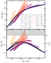 |
Fig. 10. SHMR for each of the redshift bins in this work. This was obtained by doing abundance matching using the best-fit functional forms of the SMF and the HMF by Watson et al. (2013). The top panel shows stellar mass as a function of the inferred halo mass, while the bottom panel shows the ratio between the two as a function of halo mass. The right axis indicates the SFE, |
An evolving SFE and the upturn at z ∼ 3.5 is an important feature our analysis reveals (Paquereau et al. 2025), because it provides an observational imprint of all the processes involved in regulating galaxy growth. It suggests that the SFE is not constant and that galaxies and halos do not grow at the same rate over cosmic history. A relatively simple explanation can be given in the framework of the gas-regulated model of galaxies, closely coupled with halo evolution (Lilly et al. 2013). The cosmic SFE is tightly linked to the interplay between the halo growth rate (that quantifies the growth through accretion of dark matter) and the star formation rate (that quantifies the conversion of the gas reservoir into stars).
Our results indicate that from the earliest times until z ∼ 3.5, the halo growth rate ̇Mh outpaces the SFR of the residing galaxies, causing the decrease in SFE with time. The halo growth rate slows down, while the gas reservoirs built over time in the halo can keep the SFR going and at z ≲ 3.5, galaxies outpace halo growth, resulting in the increase in the SFE. This is especially the case at Mh ≲ 1012 M⊙, in the regime where halo mass quenching has not occurred. Indeed, Paquereau et al. (2025) analyze the ratio SFR/̇Mh in UNIVERSEMACHINE and find that it decreases from 0 < z < 3.8 turns at z ∼ 3.8 and increases at higher redshifts – consistent with our observations and interpretations.
Figure 11 shows another rendering of our SHMR measurements, where redshift bins are separated in different panels for clarity, and where we compare with Shuntov et al. (2022), and the UNIVERSEMACHINE and FFB models. In general, there is very good agreement at lower redshifts, with a notable exception in the first three bins at z < 1.1. Our SHMR is consistently higher by ∼0.4 dex at the low mass end, and the peak is at lower halo mass compared to UNIVERSEMACHINE and Shuntov et al. (2022). This can be a systematic from the simplistic AM using the Mh, as opposed to other more tightly correlated halo properties. At higher redshifts (out to z ∼ 7) the low mass end remains in good agreement, with the high mass end being increasingly higher compared to UNIVERSEMACHINE, but in agreement with Shuntov et al. (2022) within the uncertainties. The sharp rise of the SHMR after z ≳ 4 in our work is in striking contrast to the UNIVERSEMACHINE model that shows a decrease. The FFB predictions are shown in the transparent envelope that enclose maximum SFE in the range of  . The FFB regime becomes important at the very high masses at lower redshifts and moves toward affecting lower masses at high redshifts, where it can reach maximum SFE at Mh ≈ 1012 M⊙ at z ∼ 6 and Mh ≈ 1011 M⊙ by z ∼ 10. In all cases, our measurements are enclosed by the
  FFB predictions. However, the increase in our SHMR toward larger values and potentially its steepening with redshift indicates that
  should be increasing with both redshift and halo mass.
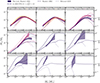 |
Fig. 11. SHMR and the implied SFE in different redshift bins. The right axis indicates the SFE, |
6.7. Tracing the SFE and stellar mass growth throughout the halo history
We used our results on the SHMR coupled with evolutionary tracks of the halo growth to study the evolution of the SFE and stellar mass within a given halo throughout cosmic history. For this purpose, we used the Dekel et al. (2013) halo growth parametrization to compute the evolution of Mh with redshift. We chose three halos of the same initial mass, Mh = 2 × 10¹¹ M⊙, starting their evolution at z = 9.3, z = 6.0, and z = 2.25, respectively. Then, at the median of each redshift bin, we computed the Mh(z) and took the SFE at that Mh from our SHMR measurements. We chose Mh = 2 × 10¹¹ M⊙ because it is the only mass probed at all redshifts (Fig. 10).
In Fig. 12 (left), we plot the evolution of the SFE in the three halos as a function of their mass and redshift. The Mh = 2 × 10¹¹ M⊙ halo starting at z = 9.3 is massive for its epoch and has a very high SFE ∼0.8, meaning is efficiently converting most of the available baryons to stars. Since the halo growth is proportional to its mass, it grows rapidly, reaches Mh ≈ 1012.5 M⊙ and enters into the hot halo mode already at z ∼ 5. This results in a sharp decline in the SFE down to 0.001 at z ∼ 0.3 in a supercluster halo of Mh ≈ 5 × 10¹⁵ M⊙. A halo of the same initial mass starting its growth at z ∼ 6, has a lower starting SFE that remains roughly constant, with only a mild increase of about 0.5 dex until cosmic noon, reaching ϵ⋆ ≈ 0.1, and then decreases by about the same amount since. In both scenarios the downturn in SFE happens after the halo has reached a similar mass-scale of ≈1012.5 M⊙, consistent with hot halo powered by AGN feedback (Gabor & Davé 2015). This is somehow higher than the characteristic ∼1012 M⊙ (Cattaneo et al. 2006), but consistent with the cold stream paradigm – at higher redshifts, cold streams can efficiently penetrate massive hot halos and fuel an increased SFE (Dekel et al. 2009). In the third case, the halo of the same initial mass at z ∼ 2.3 has the lowest starting SFE ∼0.02, which increases steadily to ϵ⋆ ∼ 0.2, a result of the slow halo growth of only about 0.6 dex in ∼5.3 Gyr.
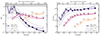 |
Fig. 12. Evolution of the SFE and stellar mass in dark matter halos, tracing the halo growth with cosmic time. Left: Evolution of the SFE for three different halos of the same initial mass, Mh = 2 × 10¹¹ M⊙, starting their evolution at z = 9.3, z = 6.0, and z = 2.25, respectively. The halo mass growth follows Dekel et al. (2013) parametrization, and the SFE is computed from the SHMR at the corresponding redshift and halo mass. The size of the points corresponds to the halo mass, also annotated above each point (in log scale). Right: Stellar mass growth in the same halos as the left panel, where M⋆ = Mh ϵ⋆ fb. The envelope corresponds to the 1σ confidence interval propagated from the uncertainty in the SHMR. The dashed lines are computed in the same way, using the resulting SHMR from the FFB model at |


In Fig. 12 (right), we show the stellar mass growth in the three halos, which we obtained in the same way as in the left panel, using M⋆ = Mh ϵ⋆ fb. The high SFE at z ∼ 9 means high stellar content (∼2 × 10¹⁰ M⊙) that sharply increases by about 1.5 dex in ∼3 Gyr after which it stagnates and reaches a maximum of ∼1012 M⊙. This would mean that in such an early and massive halo, a galaxy as massive as some of the brightest cluster galaxies (BCG) in the local Universe (Bellstedt et al. 2016) would be assembled by z ∼ 3.5. However, in these massive halos, new stellar mass likely accumulates in satellite galaxies, which is not reflected in the SHMR from AM that only considers central galaxies. The more moderate but constant SFE of the z ∼ 6 halo shows a longer and steadier stellar mass buildup of almost 2 dex until z ∼ 2 and a slower growth of about 0.2 dex since, to reach 1012 M⊙ at z ∼ 0.3. In this case, the galaxy and its host halo grow at the same rate. Finally, in the halo starting at z ∼ 2.2, the stellar growth outpaces the halo, thanks to the increasing SFE, with a 0.6 versus 1.5 dex increase in the halo and stellar mass, respectively. These trends are a signature of the downsizing scenario (De Lucia et al. 2006; Thomas et al. 2010) – the massive and early-type galaxies today have stellar populations that are formed earlier in a short period of high SFE in some of the most massive halos for its epoch.
The shape evolutionary tracks we obtain in this analysis are a result of the evolving SFE, the upturn at z ∼ 3.5 and galaxies not closely following halo growth. We can see that the SFE of a 1012 M⊙ halo decreases from the z = 10 to the z = 6 track, but then increases again for the z = 2 track. Consequently, a halo starting its growth at z > 3.5 would assemble the most stellar mass by the time it reaches Mh ≈ 1012.5 M⊙, compared to similar halos that start their growth earlier. This can be explained within the same gas-regulated model coupled with halo evolution framework that we discussed in the previous subsection, where after z ∼ 3.5 the stagnating halo growth and the available gas reservoir keep the SFE high.
In Fig. 12, we also compare with the predictions from the FFB model, obtained in the same way. The transparent envelope encloses between the no FFB regime and maximum FFB efficiency  . The FFB, as expected, has the most impact in the halo that starts its growth early. Our results for the earliest are in best agreement with
  . For the halos at lower redshifts, the FFB has no impact and the underlying UNIVERSEMACHINE model is consistently lower by 0.1–0.3 dex. However, as discussed previously, the highest redshift points do suggest an increasing
  .
.
We have to note that beyond Mh ∼ 1014, these results are based on extrapolations of the SHMR at high masses. Furthermore, the SHMR from our simple AM application relates only the mass of the (sub)halo to the mass of the central galaxy. It has been shown that beyond the cluster scale halo mass of Mh ≳ 1013 M⊙, satellite galaxies dominate the stellar mass budget of the halo (Leauthaud et al. 2012; Coupon et al. 2015; Shuntov et al. 2022). Therefore, the resulting SFE would be higher at the high-mass end if satellites were considered in the analysis.
7. Conclusions
In this paper, we have presented measurements of the SMF from JWST in 97% of cosmic history (0.2 < z < 12.0). We have leveraged the largest contiguous JWST imaging survey over ∼0.5 deg2, COSMOS-Web, along with the wealth of ground- and space-based data in COSMOS, to construct complete samples that probe a very large dynamic range in stellar mass. The large area has allowed us to study the evolution of some of the most massive and rare galaxies in the Universe. We summarize our main findings as follows.
7.1. Evolution of the SMF
-
The normalization of the GSMF monotonically decreases from z = 0.2 to z = 12, with a strong mass-dependent evolution. The density evolution at masses just below the knee (log M⋆/M⊙ ∼ 10.4) is faster than the low-mass density evolution (log M⋆/M⊙ ∼ 7), with ∼3 dex and ∼2 dex change since z ∼ 7, respectively. Beyond the knee (log M⋆/M⊙ ≳ 11), the number densities are within 1.5 dex, since z ∼ 5.
-
Our measurements show an excellent agreement with pre-JWST results at low and intermediate redshifts, and good agreement with the latest JWST results from deeper but smaller surveys. Our results corroborate the findings of increased abundances of massive galaxies at high redshifts.
-
The double Schechter function provides the best fit out to z = 3.5, the single Schechter the best fit out to z = 5.5, and the DPL the best fit at z > 5.5, due to a flattening of the high-mass end. This flattening indicates that the most massive galaxies assembled very efficiently in the first few gigayears and did not grow significantly after that, suggesting an onset of negative feedback in massive galaxies at z ∼ 5.5.
7.2. Evolution of the SMD and the inferred SFRD
-
The cosmic SMD shows a steady increase with redshift at 1 < z < 9, with no significant change in slope, indicating that stellar mass has assembled at a constant rate as a function of redshift, throughout most of cosmic history.
-
We inferred the cosmic SFRD by integrating and fitting a parametric form to the SMD measurements. At z ≲ 3.5, we find lower values of the SFRD inferred from the SMD compared to instantaneous SFR indicators, corroborating the tension between the two repeatedly reported in the past. The causes remain poorly understood, the most likely being uncertain SFR calibration factors, effects of dust attenuation, and SED modeling systematics on stellar mass and SFR measurements.
-
At z > 7.5, we find good agreement with recent JWST UVLF measurements. This remarkable consistency solidifies the emerging picture of rapid galaxy formation leading to increased abundances of bright and massive galaxies in the first ∼0.7 Gyr.
7.3. The most massive galaxies in COSMOS
-
We applied the EVS to search for the most extreme sources for their epoch, and found about 40 galaxies with masses that exceed the limits from halo abundances and local-Universe SFE factors. These are red, extended, and likely highly dust-attenuated, with properties that are difficult to estimate from optical-NIR SED fitting, and as such warrant further investigation. However, we do not report any tension with ΛCDM within the confidence intervals.
7.4. Stellar-to-halo mass relation and the integrated star formation efficiency
-
Using abundance matching, we inferred the SHMR in 15 redshift bins from z = 0.2 to z ∼ 12, finding a non-monotonic evolution, suggesting that galaxies and halos do not grow at the same rate throughout cosmic history. The integrated SFE has the characteristic strong dependence with mass and mildly decreasing trend at the low-mass end out to z ∼ 3.5 in the range of 0.02 < ϵ⋆ < 0.2.
-
After z > 3.5, the SFE increases sharply, going from ϵ⋆ ≈ 0.1 to ϵ⋆ ≈ 0.8 − 1 at z ≈ 10 for log(Mh/M⊙)≈11.5, albeit with large uncertainties. The upturn at z ∼ 3.5 indicates that halo growth rate dominates over the SFR until z ∼ 3.5, when it slows down, but accumulated gas reservoirs can keep the SFR high until the present day, resulting in a rising SFE.
-
The SHMR, coupled with halo growth curves, shows that a halo of initial mass Mh = 1011 M⊙ starting its growth at z < 3.5 would assemble the most stellar mass by the time it reaches Mh = 1012.5 M⊙. This suggests that the stagnating halo growth after z ∼ 3.5 and the available gas reservoir result in efficient SF for longer periods.
7.5. Implications for galaxy formation models
-
The comparison of the SMF with the simulation shows a good agreement out to z ∼ 6 − 7; at higher redshifts, our measurements show increasingly higher abundances with both mass and redshift.
-
We investigated several proposed theoretical models that explain the increased abundances at high redshift. We find that the FFB model can successfully reproduce our observations, but requires increasing maximum FFB efficiency with both redshift (from z > 6) and mass. Furthermore, qualitatively, our results are also consistent with the positive feedback scenario, as is indicated by the Schechter to DPL transition at z ∼ 6 and the monotonic increase in the SFE close to 80 − 100% with mass.
7.6. Future prospects
Confirmation of the high-redshift candidates from spectroscopy will be crucial to accurately measure abundances of massive galaxies and put robust constraints on the emerging theoretical models. We identify that the way forward is a complete spectroscopic survey of massive galaxies at high redshift in the COSMOS, which will also allow for robust clustering measurements deep into epoch of reionization. Halo occupation distribution analysis of the clustering and abundance measurements will put robust constrains on the host halo mass and galaxy bias at these redshifts, and unveil the true nature of the increased abundance of massive galaxies.
Data availability
To make our results transparent and facilitate comparison we provide all our measurements in tabulated form at https://github.com/mShuntov/SMF_in_COSMOS-Web_Shuntov2024, as well as at https://zenodo.org/records/14712538.
Appendices A–G are available at https://zenodo.org/records/14723773.
We provide our SMF measurements in tabulated form at https://github.com/mShuntov/SMF_in_COSMOS-Web_Shuntov2024
Which are not necessarily classified as quiescent given a sharp cut in sSFR or color. Instead, the double Schechter is a result of mixing populations with intermediate to low SF activity, and therefore can be observed even for the SMF of active galaxies (e.g., Ilbert et al. 2013; Davidzon et al. 2017; Weaver et al. 2023).
Here, it is important to make the distinction between the integrated SFE ϵ⋆ = M⋆/(Mh fb) that we use in this work, instantaneous SFE ϵ = SFR/(fb Ṁh), and the SFE in the context of gas depletion ϵgas = SFR/Mgas. Given the fact that SHMR ≡ M⋆/Mh = ϵ⋆ fb, we use the SMHR and ϵ⋆ interchangeably to refer to the integrated SFE.
Acknowledgments
The Cosmic Dawn Center (DAWN) is funded by the Danish National Research Foundation (DNRF140). This work has received funding from the Swiss State Secretariat for Education, Research, and Innovation (SERI) under contract number MB22.00072 This work was made possible thanks to the CANDIDE cluster at the Institut d’Astrophysique de Paris, which was funded through grants from the PNCG, CNES, DIM-ACAV, and the Cosmic Dawn Center; CANDIDE is maintained by S. Rouberol. The French contingent of the COSMOS team is partly supported by the Centre National d’Etudes Spatiales (CNES). OI acknowledges the funding of the French Agence Nationale de la Recherche for the project iMAGE (grant ANR-22-CE31-0007). Some of the data products presented herein were retrieved from the Dawn JWST Archive (DJA). DJA is an initiative of the Cosmic Dawn Center, which is funded by the Danish National Research Foundation under grant DNRF140. Based on observations collected at the European Southern Observatory under ESO programmes 179.A-2005, 198.A-2003, 1104.A-0643, 110.25A2 and 284.A-5026 and on data obtained from the ESO Science Archive Facility with DOI https://doi.org/10.18727/archive/52, and on data products produced by CANDIDE and the Cambridge Astronomy Survey Unit on behalf of the UltraVISTA consortium.
References
- Aihara, H., Arimoto, N., Armstrong, R., et al. 2018, PASJ, 70, S4 [NASA ADS] [Google Scholar]
- Aihara, H., AlSayyad, Y., Ando, M., et al. 2022, PASJ, 74, 247 [NASA ADS] [CrossRef] [Google Scholar]
- Akins, H. B., Casey, C. M., Allen, N., et al. 2023, ApJ, 956, 61 [NASA ADS] [CrossRef] [Google Scholar]
- Akins, H. B., Casey, C. M., Lambrides, E., et al. 2024, ArXiv e-prints, [arXiv:2406.10341] [Google Scholar]
- Arnouts, S., Moscardini, L., Vanzella, E., et al. 2002, MNRAS, 329, 355 [Google Scholar]
- Arnouts, S., Le Floc’h, E., Chevallard, J., et al. 2013, A&A, 558, A67 [NASA ADS] [CrossRef] [EDP Sciences] [Google Scholar]
- Baldry, I. K., Driver, S. P., Loveday, J., et al. 2012, MNRAS, 421, 621 [NASA ADS] [Google Scholar]
- Barrufet, L., Oesch, P. A., Weibel, A., et al. 2023, MNRAS, 522, 449 [NASA ADS] [CrossRef] [Google Scholar]
- Behroozi, P., & Silk, J. 2018, MNRAS, 477, 5382 [Google Scholar]
- Behroozi, P. S., Wechsler, R. H., & Conroy, C. 2013, ApJ, 770, 57 [NASA ADS] [CrossRef] [Google Scholar]
- Behroozi, P., Wechsler, R. H., Hearin, A. P., & Conroy, C. 2019, MNRAS, 488, 3143 [NASA ADS] [CrossRef] [Google Scholar]
- Bell, E. F., McIntosh, D. H., Katz, N., & Weinberg, M. D. 2003, ApJS, 149, 289 [Google Scholar]
- Bellstedt, S., Lidman, C., Muzzin, A., et al. 2016, MNRAS, 460, 2862 [Google Scholar]
- Bertin, E., Schefer, M., Apostolakos, N., et al. 2020, in Astronomical Data Analysis Software and Systems XXIX, eds. R. Pizzo, E. R. Deul, J. D. Mol, J. de Plaa, & H. Verkouter, Astronomical Society of the Pacific Conference Series, 527, 461 [NASA ADS] [Google Scholar]
- Bhatawdekar, R., Conselice, C. J., Margalef-Bentabol, B., & Duncan, K. 2019, MNRAS, 486, 3805 [NASA ADS] [CrossRef] [Google Scholar]
- Boquien, M., Burgarella, D., Roehlly, Y., et al. 2019, A&A, 622, A103 [NASA ADS] [CrossRef] [EDP Sciences] [Google Scholar]
- Bouwens, R. J., Illingworth, G. D., Oesch, P. A., et al. 2012a, ApJ, 754, 83 [Google Scholar]
- Bouwens, R. J., Illingworth, G. D., Oesch, P. A., et al. 2012b, ApJ, 752, L5 [Google Scholar]
- Bouwens, R. J., Stefanon, M., Brammer, G., et al. 2023a, MNRAS, 523, 1036 [NASA ADS] [CrossRef] [Google Scholar]
- Bouwens, R., Illingworth, G., Oesch, P., et al. 2023b, MNRAS, 523, 1009 [NASA ADS] [CrossRef] [Google Scholar]
- Bowler, R. A. A., Dunlop, J. S., McLure, R. J., et al. 2012, MNRAS, 426, 2772 [NASA ADS] [CrossRef] [Google Scholar]
- Bowler, R. A. A., Dunlop, J. S., McLure, R. J., et al. 2014, MNRAS, 440, 2810 [NASA ADS] [CrossRef] [Google Scholar]
- Bowler, R. A. A., Jarvis, M. J., Dunlop, J. S., et al. 2020, MNRAS, 493, 2059 [Google Scholar]
- Boylan-Kolchin, M. 2023, Nat. Astron., 7, 731 [NASA ADS] [CrossRef] [Google Scholar]
- Bruzual, G., & Charlot, S. 2003, MNRAS, 344, 1000 [NASA ADS] [CrossRef] [Google Scholar]
- Bushouse, H., Eisenhamer, J., Dencheva, N., et al. 2022, https://doi.org/10.5281/zenodo.7325378 [Google Scholar]
- Calzetti, D., Armus, L., Bohlin, R. C., et al. 2000, ApJ, 533, 682 [NASA ADS] [CrossRef] [Google Scholar]
- Calzetti, D., Kennicutt, R. C., Engelbracht, C. W., et al. 2007, ApJ, 666, 870 [Google Scholar]
- Capak, P., Mobasher, B., Scoville, N. Z., et al. 2011, ApJ, 730, 68 [NASA ADS] [CrossRef] [Google Scholar]
- Carnall, A. C., McLeod, D. J., McLure, R. J., et al. 2023, MNRAS, 520, 3974 [NASA ADS] [CrossRef] [Google Scholar]
- Casey, C. M., Berta, S., Béthermin, M., et al. 2012, ApJ, 761, 140 [NASA ADS] [CrossRef] [Google Scholar]
- Casey, C. M., Kartaltepe, J. S., Drakos, N. E., et al. 2023, ApJ, 954, 31 [NASA ADS] [CrossRef] [Google Scholar]
- Casey, C. M., Akins, H. B., Shuntov, M., et al. 2024, ApJ, 965, 98 [NASA ADS] [CrossRef] [Google Scholar]
- Cattaneo, A., Dekel, A., Devriendt, J., Guiderdoni, B., & Blaizot, J. 2006, MNRAS, 370, 1651 [NASA ADS] [CrossRef] [Google Scholar]
- Chabrier, G. 2003, PASP, 115, 763 [Google Scholar]
- Chworowsky, K., Finkelstein, S. L., Boylan-Kolchin, M., et al. 2024, AJ, 168, 113 [NASA ADS] [CrossRef] [Google Scholar]
- Ciesla, L., Elbaz, D., Ilbert, O., et al. 2024, A&A, 686, A128 [NASA ADS] [CrossRef] [EDP Sciences] [Google Scholar]
- Civano, F., Marchesi, S., Comastri, A., et al. 2016, ApJ, 819, 62 [Google Scholar]
- Cole, S., Norberg, P., Baugh, C. M., et al. 2001, MNRAS, 326, 255 [NASA ADS] [CrossRef] [Google Scholar]
- Conroy, C., & Wechsler, R. H. 2009, ApJ, 696, 620 [NASA ADS] [CrossRef] [Google Scholar]
- Coupon, J., Arnouts, S., van Waerbeke, L., et al. 2015, MNRAS, 449, 1352 [NASA ADS] [CrossRef] [Google Scholar]
- Cueto, E. R., Hutter, A., Dayal, P., et al. 2024, A&A, 686, A138 [NASA ADS] [CrossRef] [EDP Sciences] [Google Scholar]
- Davidzon, I., Ilbert, O., Laigle, C., et al. 2017, A&A, 605, A70 [NASA ADS] [CrossRef] [EDP Sciences] [Google Scholar]
- De Lucia, G., Springel, V., White, S. D. M., Croton, D., & Kauffmann, G. 2006, MNRAS, 366, 499 [NASA ADS] [CrossRef] [Google Scholar]
- De Lucia, G., Fontanot, F., Xie, L., & Hirschmann, M. 2024, A&A, 687, A68 [NASA ADS] [CrossRef] [EDP Sciences] [Google Scholar]
- Dekel, A., Birnboim, Y., Engel, G., et al. 2009, Nature, 457, 451 [Google Scholar]
- Dekel, A., Zolotov, A., Tweed, D., et al. 2013, MNRAS, 435, 999 [Google Scholar]
- Dekel, A., Sarkar, K. C., Birnboim, Y., Mandelker, N., & Li, Z. 2023, MNRAS, 523, 3201 [NASA ADS] [CrossRef] [Google Scholar]
- Donnan, C. T., McLeod, D. J., Dunlop, J. S., et al. 2023, MNRAS, 518, 6011 [Google Scholar]
- Donnan, C. T., McLure, R. J., Dunlop, J. S., et al. 2024, MNRAS, 533, 3222 [NASA ADS] [CrossRef] [Google Scholar]
- Drakos, N. E., Villasenor, B., Robertson, B. E., et al. 2022, ApJ, 926, 194 [NASA ADS] [CrossRef] [Google Scholar]
- Drlica-Wagner, A., Sevilla-Noarbe, I., Rykoff, E. S., et al. 2018, ApJS, 235, 33 [Google Scholar]
- Duan, Q., Conselice, C. J., Li, Q., et al. 2024, ArXiv e-prints [arXiv:2407.09472] [Google Scholar]
- Dubois, Y., Rodríguez Montero, F., Guerra, C., et al. 2024, A&A, 687, A240 [NASA ADS] [CrossRef] [EDP Sciences] [Google Scholar]
- Dunlop, J. S., Abraham, R. G., Ashby, M. L. N., et al. 2021, PRIMER: Public Release IMaging for Extragalactic Research, JWST Proposal. Cycle 1, ID. #1837 [Google Scholar]
- Dunlop, J. S., Bowler, R. A. A., Franx, M., et al. 2023, https://doi.org/10.5281/zenodo.10150386 [Google Scholar]
- Eddington, A. S. 1913, MNRAS, 73, 359 [Google Scholar]
- Euclid Collaboration (McPartland, C. J. R., et al.) 2025, A&A, in press, https://doi.org/10.1051/0004-6361/202451849 [Google Scholar]
- Feng, Y., Di-Matteo, T., Croft, R. A., et al. 2016, MNRAS, 455, 2778 [NASA ADS] [CrossRef] [Google Scholar]
- Finkelstein, S. L., & Bagley, M. B. 2022, ApJ, 938, 25 [NASA ADS] [CrossRef] [Google Scholar]
- Finkelstein, S. L., Leung, G. C. K., Bagley, M. B., et al. 2024, ApJ, 969, L2 [NASA ADS] [CrossRef] [Google Scholar]
- Fontana, A., Salimbeni, S., Grazian, A., et al. 2006, A&A, 459, 745 [CrossRef] [EDP Sciences] [Google Scholar]
- Foreman-Mackey, D., Hogg, D. W., Lang, D., & Goodman, J. 2013, PASP, 125, 306 [Google Scholar]
- Franco, M., Akins, H. B., Casey, C. M., et al. 2024, ApJ, 973, 23 [NASA ADS] [CrossRef] [Google Scholar]
- Fujimoto, S., Arrabal Haro, P., Dickinson, M., et al. 2023, ApJ, 949, L25 [NASA ADS] [CrossRef] [Google Scholar]
- Furtak, L. J., Shuntov, M., Atek, H., et al. 2023, MNRAS, 519, 3064 [Google Scholar]
- Gabor, J. M., & Davé, R. 2015, MNRAS, 447, 374 [NASA ADS] [CrossRef] [Google Scholar]
- Gehrels, N. 1986, ApJ, 303, 336 [Google Scholar]
- Gelli, V., Mason, C., & Hayward, C. C. 2024, ApJ, 975, 192 [NASA ADS] [CrossRef] [Google Scholar]
- Gentile, F., Casey, C. M., Akins, H. B., et al. 2024, ApJ, 973, L2 [NASA ADS] [CrossRef] [Google Scholar]
- Giménez-Arteaga, C., Oesch, P. A., Brammer, G. B., et al. 2023, ApJ, 948, 126 [CrossRef] [Google Scholar]
- Gottumukkala, R., Barrufet, L., Oesch, P. A., et al. 2024, MNRAS, 530, 966 [NASA ADS] [CrossRef] [Google Scholar]
- Grazian, A., Fontana, A., Santini, P., et al. 2015, A&A, 575, A96 [NASA ADS] [CrossRef] [EDP Sciences] [Google Scholar]
- Greene, J. E., Labbe, I., Goulding, A. D., et al. 2024, ApJ, 964, 39 [CrossRef] [Google Scholar]
- Grudić, M. Y., Hopkins, P. F., Faucher-Giguère, C.-A., et al. 2018, MNRAS, 475, 3511 [CrossRef] [Google Scholar]
- Hainline, L. J., Blain, A. W., Smail, I., et al. 2011, ApJ, 740, 96 [NASA ADS] [CrossRef] [Google Scholar]
- Harikane, Y., Ono, Y., Ouchi, M., et al. 2022, ApJS, 259, 20 [NASA ADS] [CrossRef] [Google Scholar]
- Harikane, Y., Zhang, Y., Nakajima, K., et al. 2023a, ApJ, 959, 39 [NASA ADS] [CrossRef] [Google Scholar]
- Harikane, Y., Ouchi, M., Oguri, M., et al. 2023b, ApJS, 265, 5 [NASA ADS] [CrossRef] [Google Scholar]
- Harvey, T., Conselice, C. J., Adams, N. J., et al. 2025, ApJ, 978, 89 [NASA ADS] [CrossRef] [Google Scholar]
- Hasinger, G., Capak, P., Salvato, M., et al. 2018, ApJ, 858, 77 [Google Scholar]
- Haskell, P., Smith, D. J. B., Cochrane, R. K., Hayward, C. C., & Anglés-Alcázar, D. 2023, MNRAS, 525, 1535 [NASA ADS] [CrossRef] [Google Scholar]
- Haskell, P., Das, S., Smith, D. J. B., et al. 2024, MNRAS, 530, L7 [NASA ADS] [CrossRef] [Google Scholar]
- Hayward, C. C., & Smith, D. J. B. 2015, MNRAS, 446, 1512 [Google Scholar]
- Helton, J. M., Sun, F., Woodrum, C., et al. 2024, ApJ, 974, 41 [Google Scholar]
- Hopkins, A. M., & Beacom, J. F. 2006, ApJ, 651, 142 [NASA ADS] [CrossRef] [Google Scholar]
- Hutter, A., Dayal, P., Yepes, G., et al. 2021, MNRAS, 503, 3698 [NASA ADS] [CrossRef] [Google Scholar]
- Ilbert, O., Arnouts, S., McCracken, H. J., et al. 2006, A&A, 457, 841 [NASA ADS] [CrossRef] [EDP Sciences] [Google Scholar]
- Ilbert, O., McCracken, H. J., Le Fèvre, O., et al. 2013, A&A, 556, A55 [NASA ADS] [CrossRef] [EDP Sciences] [Google Scholar]
- Ilbert, O., Arnouts, S., Le Floc’h, E., et al. 2015, A&A, 579, A2 [NASA ADS] [CrossRef] [EDP Sciences] [Google Scholar]
- Jespersen, C. K., Cranmer, M., Melchior, P., et al. 2022, ApJ, 941, 7 [NASA ADS] [CrossRef] [Google Scholar]
- Jespersen, C. K., Steinhardt, C. L., Somerville, R. S., & Lovell, C. C. 2024, ArXiv e-prints [arXiv:2403.00050] [Google Scholar]
- Jin, S., Daddi, E., Magdis, G. E., et al. 2019, ApJ, 887, 144 [Google Scholar]
- Johnston, R. 2011, A&ARv, 19, 41 [NASA ADS] [CrossRef] [Google Scholar]
- Kartaltepe, J. S., Sanders, D. B., Le Floc’h, E., et al. 2010, ApJ, 721, 98 [NASA ADS] [CrossRef] [Google Scholar]
- Kartaltepe, J. S., Sanders, D. B., Silverman, J. D., et al. 2015, ApJ, 806, L35 [NASA ADS] [CrossRef] [Google Scholar]
- Kashino, D., Silverman, J. D., Sanders, D., et al. 2019, ApJS, 241, 10 [Google Scholar]
- Kennicutt, R. C., Jr. 1998, ApJ, 498, 541 [Google Scholar]
- Klypin, A., Poulin, V., Prada, F., et al. 2021, MNRAS, 504, 769 [NASA ADS] [CrossRef] [Google Scholar]
- Kocevski, D. D., Onoue, M., Inayoshi, K., et al. 2023, ApJ, 954, L4 [NASA ADS] [CrossRef] [Google Scholar]
- Koekemoer, A. M., Aussel, H., Calzetti, D., et al. 2007, ApJS, 172, 196 [Google Scholar]
- Kokorev, V., Caputi, K. I., Greene, J. E., et al. 2024, ApJ, 968, 38 [NASA ADS] [CrossRef] [Google Scholar]
- Kravtsov, A. V., Berlind, A. A., Wechsler, R. H., et al. 2004, ApJ, 609, 35 [Google Scholar]
- Kriek, M., Shapley, A. E., Reddy, N. A., et al. 2015, ApJS, 218, 15 [NASA ADS] [CrossRef] [Google Scholar]
- Kümmel, M., Bertin, E., Schefer, M., et al. 2020, in Astronomical Data Analysis Software and Systems XXIX, eds. R. Pizzo, E. R. Deul, J. D. Mol, J. de Plaa, & H. Verkouter, Astronomical Society of the Pacific Conference Series, 527, 29 [Google Scholar]
- Labbé, I., van Dokkum, P., Nelson, E., et al. 2023, Nature, 616, 266 [CrossRef] [Google Scholar]
- Labbe, I., Greene, J. E., Bezanson, R., et al. 2025, ApJ, 978, 92 [NASA ADS] [CrossRef] [Google Scholar]
- Le Fèvre, O., Tasca, L. A. M., Cassata, P., et al. 2015, A&A, 576, A79 [Google Scholar]
- Leauthaud, A., Tinker, J., Bundy, K., et al. 2012, ApJ, 744, 159 [Google Scholar]
- Legrand, L., McCracken, H. J., Davidzon, I., et al. 2019, MNRAS, 486, 5468 [NASA ADS] [CrossRef] [Google Scholar]
- Leja, J., van Dokkum, P. G., Franx, M., & Whitaker, K. E. 2015, ApJ, 798, 115 [NASA ADS] [CrossRef] [Google Scholar]
- Leja, J., Speagle, J. S., Johnson, B. D., et al. 2020, ApJ, 893, 111 [Google Scholar]
- Li, Z., Dekel, A., Sarkar, K. C., et al. 2024, A&A, 690, A108 [NASA ADS] [CrossRef] [EDP Sciences] [Google Scholar]
- Lilly, S. J., Le Brun, V., Maier, C., et al. 2009, ApJS, 184, 218 [Google Scholar]
- Lilly, S. J., Carollo, C. M., Pipino, A., Renzini, A., & Peng, Y. 2013, ApJ, 772, 119 [NASA ADS] [CrossRef] [Google Scholar]
- Liu, D., Schinnerer, E., Groves, B., et al. 2019, ApJ, 887, 235 [Google Scholar]
- Liu, W., Zhan, H., Gong, Y., & Wang, X. 2024, MNRAS, 533, 860 [NASA ADS] [CrossRef] [Google Scholar]
- Lovell, C. C., Vijayan, A. P., Thomas, P. A., et al. 2021, MNRAS, 500, 2127 [Google Scholar]
- Lovell, C. C., Harrison, I., Harikane, Y., Tacchella, S., & Wilkins, S. M. 2023, MNRAS, 518, 2511 [Google Scholar]
- Madau, P. 1995, ApJ, 441, 18 [NASA ADS] [CrossRef] [Google Scholar]
- Madau, P., & Dickinson, M. 2014, ARA&A, 52, 415 [Google Scholar]
- Madau, P., Pozzetti, L., & Dickinson, M. 1998, ApJ, 498, 106 [NASA ADS] [CrossRef] [Google Scholar]
- Maiolino, R., Scholtz, J., Curtis-Lake, E., et al. 2024, A&A, 691, A145 [NASA ADS] [CrossRef] [EDP Sciences] [Google Scholar]
- Malmquist, K. G. 1922, Lund Medd, 100, 1 [NASA ADS] [Google Scholar]
- Marchesini, D., van Dokkum, P. G., Förster Schreiber, N. M., et al. 2009, ApJ, 701, 1765 [NASA ADS] [CrossRef] [Google Scholar]
- Marinacci, F., Vogelsberger, M., Pakmor, R., et al. 2018, MNRAS, 480, 5113 [NASA ADS] [Google Scholar]
- Marinoni, C., & Hudson, M. J. 2002, ApJ, 569, 101 [NASA ADS] [CrossRef] [Google Scholar]
- Matthee, J., Naidu, R. P., Brammer, G., et al. 2024, ApJ, 963, 129 [NASA ADS] [CrossRef] [Google Scholar]
- McCracken, H. J., Milvang-Jensen, B., Dunlop, J., et al. 2012, A&A, 544, A156 [NASA ADS] [CrossRef] [EDP Sciences] [Google Scholar]
- McKinney, J., Casey, C. M., Long, A. S., et al. 2024, ArXiv e-prints [arXiv:2408.08346] [Google Scholar]
- McLeod, D. J., McLure, R. J., Dunlop, J. S., et al. 2021, MNRAS, 503, 4413 [NASA ADS] [CrossRef] [Google Scholar]
- Michałowski, M. J., Dunlop, J. S., Cirasuolo, M., et al. 2012, A&A, 541, A85 [NASA ADS] [CrossRef] [EDP Sciences] [Google Scholar]
- Milvang-Jensen, B., Freudling, W., Zabl, J., et al. 2013, A&A, 560, A94 [NASA ADS] [CrossRef] [EDP Sciences] [Google Scholar]
- Mitchell, P. D., Lacey, C. G., Baugh, C. M., & Cole, S. 2013, MNRAS, 435, 87 [NASA ADS] [CrossRef] [Google Scholar]
- Moster, B. P., Somerville, R. S., Newman, J. A., & Rix, H.-W. 2011, ApJ, 731, 113 [Google Scholar]
- Moutard, T., Arnouts, S., Ilbert, O., et al. 2016, A&A, 590, A103 [NASA ADS] [CrossRef] [EDP Sciences] [Google Scholar]
- Muzzin, A., Marchesini, D., Stefanon, M., et al. 2013, ApJ, 777, 18 [NASA ADS] [CrossRef] [Google Scholar]
- Naiman, J. P., Pillepich, A., Springel, V., et al. 2018, MNRAS, 477, 1206 [Google Scholar]
- Narayanan, D., Lower, S., Torrey, P., et al. 2024, ApJ, 961, 73 [NASA ADS] [CrossRef] [Google Scholar]
- Navarro-Carrera, R., Rinaldi, P., Caputi, K. I., et al. 2023, ArXiv e-prints [arXiv:2305.16141] [Google Scholar]
- Nelson, D., Pillepich, A., Springel, V., et al. 2018, MNRAS, 475, 624 [Google Scholar]
- Oke, J. B., & Gunn, J. E. 1983, ApJ, 266, 713 [NASA ADS] [CrossRef] [Google Scholar]
- Pacifici, C., Iyer, K. G., Mobasher, B., et al. 2023, ApJ, 944, 141 [NASA ADS] [CrossRef] [Google Scholar]
- Pallottini, A., & Ferrara, A. 2023, A&A, 677, L4 [NASA ADS] [CrossRef] [EDP Sciences] [Google Scholar]
- Paquereau, L., Laigle, C., McCracken, H. J., et al. 2025, ArXiv e-prints [arXiv:2501.11674] [Google Scholar]
- Peng, Y.-J., Lilly, S. J., Kovač, K., et al. 2010, ApJ, 721, 193 [Google Scholar]
- Pérez-González, P. G., Costantin, L., Langeroodi, D., et al. 2023, ApJ, 951, L1 [CrossRef] [Google Scholar]
- Pillepich, A., Nelson, D., Hernquist, L., et al. 2018, MNRAS, 475, 648 [Google Scholar]
- Pozzetti, L., Bolzonella, M., Lamareille, F., et al. 2007, A&A, 474, 443 [NASA ADS] [CrossRef] [EDP Sciences] [Google Scholar]
- Pozzetti, L., Bolzonella, M., Zucca, E., et al. 2010, A&A, 523, A13 [NASA ADS] [CrossRef] [EDP Sciences] [Google Scholar]
- Reddick, R. M., Wechsler, R. H., Tinker, J. L., & Behroozi, P. S. 2013, ApJ, 771, 30 [Google Scholar]
- Renzini, A. 2023, MNRAS, 525, L117 [NASA ADS] [CrossRef] [Google Scholar]
- Renzini, A., & Buzzoni, A. 1986, in Spectral Evolution of Galaxies, eds. C. Chiosi, & A. Renzini, Astrophys. Space Sci. Lib., 122, 195 [NASA ADS] [CrossRef] [Google Scholar]
- Robertson, B. E. 2010, ApJ, 713, 1266 [NASA ADS] [CrossRef] [Google Scholar]
- Rieke, M. J., Kelly, D., & Horner, S., 2005, SPIE Conf. Ser., 5904, 1 [NASA ADS] [Google Scholar]
- Saito, S., de la Torre, S., Ilbert, O., et al. 2020, MNRAS, 494, 199 [NASA ADS] [CrossRef] [Google Scholar]
- Salim, S., Boquien, M., & Lee, J. C. 2018, ApJ, 859, 11 [Google Scholar]
- Sawicki, M., Arnouts, S., Huang, J., et al. 2019, MNRAS, 489, 5202 [NASA ADS] [Google Scholar]
- Schaerer, D., & de Barros, S. 2009, A&A, 502, 423 [NASA ADS] [CrossRef] [EDP Sciences] [Google Scholar]
- Schechter, P. 1976, ApJ, 203, 297 [Google Scholar]
- Schmidt, M. 1968, ApJ, 151, 393 [Google Scholar]
- Schwarz, G. 1978, Ann. Stat., 6, 461 [Google Scholar]
- Scoville, N., Abraham, R. G., Aussel, H., et al. 2007, ApJS, 172, 38 [NASA ADS] [CrossRef] [Google Scholar]
- Shen, X., Vogelsberger, M., Boylan-Kolchin, M., Tacchella, S., & Kannan, R. 2023, MNRAS, 525, 3254 [NASA ADS] [CrossRef] [Google Scholar]
- Shuntov, M., McCracken, H. J., Gavazzi, R., et al. 2022, A&A, 664, A61 [NASA ADS] [CrossRef] [EDP Sciences] [Google Scholar]
- Silk, J., & Mamon, G. A. 2012, Res. Astron. Astrophys., 12, 917 [Google Scholar]
- Silk, J., Begelman, M. C., Norman, C., Nusser, A., & Wyse, R. F. G. 2024, ApJ, 961, L39 [NASA ADS] [CrossRef] [Google Scholar]
- Silverman, J. D., Kashino, D., Sanders, D., et al. 2015, ApJS, 220, 12 [NASA ADS] [CrossRef] [Google Scholar]
- Song, M., Finkelstein, S. L., Ashby, M. L. N., et al. 2016, ApJ, 825, 5 [NASA ADS] [CrossRef] [Google Scholar]
- Springel, V., Pakmor, R., Pillepich, A., et al. 2018, MNRAS, 475, 676 [Google Scholar]
- Stefanon, M., Bouwens, R. J., Labbé, I., et al. 2021, ApJ, 922, 29 [NASA ADS] [CrossRef] [Google Scholar]
- Steinhardt, C. L., Capak, P., Masters, D., & Speagle, J. S. 2016, ApJ, 824, 21 [NASA ADS] [CrossRef] [Google Scholar]
- Steinhardt, C. L., Jespersen, C. K., & Linzer, N. B. 2021, ApJ, 923, 8 [NASA ADS] [CrossRef] [Google Scholar]
- Steinhardt, C. L., Sneppen, A., Mostafa, B., et al. 2022, ApJ, 931, 58 [NASA ADS] [CrossRef] [Google Scholar]
- Steinhardt, C. L., Kokorev, V., Rusakov, V., Garcia, E., & Sneppen, A. 2023, ApJ, 951, L40 [NASA ADS] [CrossRef] [Google Scholar]
- Sun, G., Faucher-Giguère, C.-A., Hayward, C. C., et al. 2023, ApJ, 955, L35 [CrossRef] [Google Scholar]
- Szalay, A. S., Connolly, A. J., & Szokoly, G. P. 1999, AJ, 117, 68 [Google Scholar]
- Taniguchi, Y., Scoville, N., Murayama, T., et al. 2007, ApJS, 172, 9 [Google Scholar]
- Taniguchi, Y., Kajisawa, M., Kobayashi, M. A. R., et al. 2015, PASJ, 67, 104 [NASA ADS] [Google Scholar]
- Tasitsiomi, A., Kravtsov, A. V., Wechsler, R. H., & Primack, J. R. 2004, ApJ, 614, 533 [NASA ADS] [CrossRef] [Google Scholar]
- Thomas, D., Maraston, C., Schawinski, K., Sarzi, M., & Silk, J. 2010, MNRAS, 404, 1775 [NASA ADS] [Google Scholar]
- Torrey, P., Hopkins, P. F., Faucher-Giguère, C.-A., et al. 2017, MNRAS, 467, 2301 [NASA ADS] [CrossRef] [Google Scholar]
- Vale, A., & Ostriker, J. P. 2004, MNRAS, 353, 189 [Google Scholar]
- Valentino, F., Brammer, G., Gould, K. M. L., et al. 2023, ApJ, 947, 20 [NASA ADS] [CrossRef] [Google Scholar]
- Vijayan, A. P., Wilkins, S. M., Lovell, C. C., et al. 2022, MNRAS, 511, 4999 [NASA ADS] [CrossRef] [Google Scholar]
- Vujeva, L., Steinhardt, C. L., Jespersen, C. K., et al. 2024, ApJ, 974, 23 [NASA ADS] [CrossRef] [Google Scholar]
- Wang, T., Sun, H., Zhou, L., et al. 2024a, ArXiv e-prints [arXiv:2403.02399] [Google Scholar]
- Wang, B., Leja, J., de Graaff, A., et al. 2024b, ApJ, 969, L13 [NASA ADS] [CrossRef] [Google Scholar]
- Watson, W. A., Iliev, I. T., D’Aloisio, A., et al. 2013, MNRAS, 433, 1230 [Google Scholar]
- Weaver, J. R., Kauffmann, O. B., Ilbert, O., et al. 2022, ApJS, 258, 11 [NASA ADS] [CrossRef] [Google Scholar]
- Weaver, J. R., Davidzon, I., Toft, S., et al. 2023, A&A, 677, A184 [NASA ADS] [CrossRef] [EDP Sciences] [Google Scholar]
- Wechsler, R. H., & Tinker, J. L. 2018, ARA&A, 56, 435 [NASA ADS] [CrossRef] [Google Scholar]
- Weibel, A., Oesch, P. A., Barrufet, L., et al. 2024, MNRAS, 533, 1808 [NASA ADS] [CrossRef] [Google Scholar]
- Weigel, A. K., Schawinski, K., & Bruderer, C. 2016, MNRAS, 459, 2150 [NASA ADS] [CrossRef] [Google Scholar]
- White, S. D. M., & Rees, M. J. 1978, MNRAS, 183, 341 [Google Scholar]
- Wilkins, S. M., Trentham, N., & Hopkins, A. M. 2008, MNRAS, 385, 687 [NASA ADS] [CrossRef] [Google Scholar]
- Wilkins, S. M., Feng, Y., Di Matteo, T., et al. 2017, MNRAS, 469, 2517 [NASA ADS] [CrossRef] [Google Scholar]
- Wilkins, S. M., Lovell, C. C., & Stanway, E. R. 2019, MNRAS, 490, 5359 [NASA ADS] [CrossRef] [Google Scholar]
- Wilkins, S. M., Vijayan, A. P., Lovell, C. C., et al. 2023, MNRAS, 519, 3118 [Google Scholar]
- Willott, C. J., Desprez, G., Asada, Y., et al. 2024, ApJ, 966, 74 [NASA ADS] [CrossRef] [Google Scholar]
- Wright, A. H., Driver, S. P., & Robotham, A. S. G. 2018, MNRAS, 480, 3491 [Google Scholar]
- Xiao, M., Oesch, P. A., Elbaz, D., et al. 2024, Nature, 635, 311 [NASA ADS] [CrossRef] [Google Scholar]
- Yung, L. Y. A., Somerville, R. S., Popping, G., et al. 2019, MNRAS, 490, 2855 [NASA ADS] [CrossRef] [Google Scholar]
- Zavala, J. A., Casey, C. M., Manning, S. M., et al. 2021, ApJ, 909, 165 [CrossRef] [Google Scholar]
All Tables
Photo-z performance estimated using high-quality spectroscopic redshifts with > 97% confidence.
All Figures
|
Fig. 1. Magnitude number counts in COSMOS-Web and PRIMER used for completeness estimation. Top: Total magnitude number counts as a function of F444W model magnitude in the COSMOS-Web and PRIMER-COSMOS catalogs. Bottom: Completeness fraction, defined as the ratio between the number counts of COSMOS-Web vs. PRIMER. |
| In the text | |
|
Fig. 2. Photo-z vs. stellar mass diagram showing the completeness limits for the COSMOS-Web catalog. The stellar mass completeness limits were derived by rescaling the stellar masses of the 30% faintest sources to the limiting magnitude of the survey (Eq. (1)) and taking the 95th percentile of this distribution. |
| In the text | |
|
Fig. 3. Uncertainty budget of the SMF measurements. The three panels show the fractional uncertainty due to cosmic variance (left), Poisson (center), and SED fitting (right) in solid lines. The dashed lines, common to all panels, show the total uncertainty, obtained summing in quadrature the three contributions. For clarity, only a subset of our redshift bins are plotted. |
| In the text | |
|
Fig. 4. Measurements of the SMF in COSMOS-Web in all 15 redshift bins. Each color corresponds to a different redshift bin. The solid lines mark the measurements, while the filled areas envelop the 1σ confidence interval including Poisson, cosmic variance, and SED-fitting errors. The SMF monotonically decreases at all redshifts, with a strong mass-dependent evolution. |
| In the text | |
|
Fig. 5. Measurements of the SMF and its evolution with redshift in COSMOS-Web. Each panel shows the SMF in a given redshift bin, along with measurements in the literature from Weaver et al. (2022), Davidzon et al. (2017), Stefanon et al. (2021), Navarro-Carrera et al. (2023), Weibel et al. (2024), Harvey et al. (2025). The upper limits for empty bins are shown for the COSMOS-Web volume. In each z bin, we show the functional form that fits best the data (lowest Bayesian information criterion), while at z > 4.5, we show both the single Schechter and DPL fits for illustration. We plot the functions convolved with the Eddington bias kernel. |
| In the text | |
|
Fig. 6. Redshift evolution of the best-fit parameters for the Schechter (double and single) and DPL, along with a literature comparison. The different empty symbols correspond to the best-fit function adopted at a given redshift using the BIC. For illustration, at z > 5.5, we show the results from both Schechter and DPL fits. |
| In the text | |
|
Fig. 7. Cosmic evolution of the stellar mass and star formation rate density. Left: Evolution of the SMD, showing a steady increase with time, with no significant change in slope at 1 < z < 9. Results from our work are shown in the orange line (median) and envelope (1σ uncertainty) in both panels. This is computed by integrating best-fit SMF at a given redshift from a common lower limit of 108 M⊙. The comparison with some of the most recent literature results includes Moutard et al. (2016), Wright et al. (2018), Bhatawdekar et al. (2019), Leja et al. (2020), Stefanon et al. (2021), Weaver et al. (2023), Navarro-Carrera et al. (2023), Weibel et al. (2024) and Harvey et al. (2025). The dashed green line shows the ρ⋆ obtained by integrating the Madau & Dickinson (2014) SFRD function multiplied by a time-dependent return fraction based on Chabrier IMF (see Sect. 5.6). The gray lines show the theoretical limits imposed by the HMF, scaled by the baryonic fraction fb and different integrated SFEs ϵ⋆, integrated from the same 108 M⊙ limit. Right: Inferred cosmic evolution of the SFRD. Comparison with the literature includes measurements of ρSFR from UVLF from Harikane et al. (2022, 2023b), Donnan et al. (2023, 2024), Willott et al. (2024), Pérez-González et al. (2023), Bouwens et al. (2023a) and Bouwens et al. (2023b) or from IRLF by Zavala et al. (2021), as well as the compilation in Madau & Dickinson (2014). All are obtained using a common lower integration limit of the UVLF of MUV = −17, including Bouwens et al. (2023a,b) that we rescale using a factor of 0.5 dex. All points are converted to a Chabrier IMF. The ρSFR inferred from SMF measurements is also shown for a compilation of the most recent literature works (Ilbert et al. 2013; Stefanon et al. 2021; Weibel et al. 2024; Harvey et al. 2025) shown only for the best-fit function, without confidence intervals for clarity. The solid lines turn to transparent at lower z that are not probed in the corresponding work. The solid (dashed) black line and shaded region show the true (observed) SFRD from Behroozi et al. (2019). Our results indicate lower inferred SFRD at z < 3.5, in tension with instantaneous SFR indicators, while at z > 7.5 we find remarkable consistency with recent JWST UVLF results. |
| In the text | |
|
Fig. 8. Theoretical limits imposed from halo abundances of the most massive plausible galaxies at a given epoch and volume within the extreme value statistics (EVS) formalism. The colored regions indicate the EVS confidence intervals for the COSMOS-Web survey area of 0.43 deg2. The dotted line marks the median of the EVS distribution of the maximum plausible stellar mass, assuming a log-normal distribution of the SFE centered at ∼0.14, while the dashed line shows the 3σ upper limit assuming a SFE of unity. The grayscale hex bin histogram shows the M⋆ − zphot distribution of the full sample. Above the median |
| In the text | |
|
Fig. 9. Comparison of the COSMOS-Web SMF to theoretical models. Measurements and best fits from this work are shown in the orange circles and filled region. We compare with the predictions from the FFB model by Dekel et al. (2023), Li et al. (2024), which are based of UNIVERSEMACHINE (Behroozi et al. 2019) corresponding to different maximum SFEs (ϵ⋆) in the FFB regime, shown with the solid lines. We also show the SMF from a number of semi-analytical (ASTRAEUS, Hutter et al. 2021; Cueto et al. 2024; SANTA CRUZ SAM, Yung et al. 2019; DREAM, Drakos et al. 2022; GAEA De Lucia et al. 2024) and hydrodynamical simulations (BLUETIDES, Feng et al. 2016; Wilkins et al. 2017; FLARES, Lovell et al. 2021; Vijayan et al. 2022; Wilkins et al. 2023; TNG100, Springel et al. 2018; Nelson et al. 2018; Pillepich et al. 2018; Marinacci et al. 2018; Naiman et al. 2018), and the predictions of the Early Dark Energy model by Liu et al. (2024). |
| In the text | |
|
Fig. 10. SHMR for each of the redshift bins in this work. This was obtained by doing abundance matching using the best-fit functional forms of the SMF and the HMF by Watson et al. (2013). The top panel shows stellar mass as a function of the inferred halo mass, while the bottom panel shows the ratio between the two as a function of halo mass. The right axis indicates the SFE, |
| In the text | |
|
Fig. 11. SHMR and the implied SFE in different redshift bins. The right axis indicates the SFE, |
| In the text | |
|
Fig. 12. Evolution of the SFE and stellar mass in dark matter halos, tracing the halo growth with cosmic time. Left: Evolution of the SFE for three different halos of the same initial mass, Mh = 2 × 10¹¹ M⊙, starting their evolution at z = 9.3, z = 6.0, and z = 2.25, respectively. The halo mass growth follows Dekel et al. (2013) parametrization, and the SFE is computed from the SHMR at the corresponding redshift and halo mass. The size of the points corresponds to the halo mass, also annotated above each point (in log scale). Right: Stellar mass growth in the same halos as the left panel, where M⋆ = Mh ϵ⋆ fb. The envelope corresponds to the 1σ confidence interval propagated from the uncertainty in the SHMR. The dashed lines are computed in the same way, using the resulting SHMR from the FFB model at |
| In the text | |
Current usage metrics show cumulative count of Article Views (full-text article views including HTML views, PDF and ePub downloads, according to the available data) and Abstracts Views on Vision4Press platform.
Data correspond to usage on the plateform after 2015. The current usage metrics is available 48-96 hours after online publication and is updated daily on week days.
Initial download of the metrics may take a while.