| Issue |
A&A
Volume 677, September 2023
|
|
|---|---|---|
| Article Number | A103 | |
| Number of page(s) | 18 | |
| Section | Numerical methods and codes | |
| DOI | https://doi.org/10.1051/0004-6361/202347062 | |
| Published online | 12 September 2023 | |
Energy-resolved pulse profiles of accreting pulsars: Diagnostic tools for spectral features
1
Department of astronomy, University of Geneva,
chemin d’Écogia, 16,
1290
Versoix, Switzerland
e-mail: carlo.ferrigno@unige.ch
2
INAF – IASF-Palermo,
via Ugo La Malfa 153,
90146
Palermo PA, Italy
3
INAF, Osservatorio Astronomico di Brera,
Via E. Bianchi 46,
23807
Merate, Italy
Received:
31
May
2023
Accepted:
7
July
2023
Aims. We introduce a method for extracting spectral information from energy-resolved light curves folded at the neutron star spin period (known as pulse profiles) in accreting X-ray binaries. Spectra of these sources are sometimes characterized by features superimposed on a smooth continuum, such as iron emission lines and cyclotron resonant scattering features. We address here the question on how to derive quantitative constraints on such features from energy-dependent changes in the pulse profiles.
Methods. We developed a robust method for determining in each energy-selected bin the value of the pulsed fraction using the fast Fourier transform opportunely truncated at the number of harmonics needed to satisfactorily describe the actual profile. We determined the uncertainty on this value by sampling through Monte Carlo simulations a total of 1000 faked profiles. We rebinned the energy-resolved pulse profiles to have a constant minimum signal-to-noise ratio throughout the whole energy band. Finally we characterize the dependence of the energy-resolved pulsed fraction using a phenomenological polynomial model and search for features corresponding to spectral signatures of iron emission or cyclotron lines using Gaussian line profiles.
Results. We apply our method to a representative sample of NuSTAR observations of well-known accreting X-ray pulsars. We show that, with this method, it is possible to characterize the pulsed fraction spectra, and to constrain the position and widths of such features with a precision comparable with the spectral results. We also explore how harmonic decomposition, correlation, and lag spectra might be used as additional probes for detection and characterization of such features.
Key words: X-rays: binaries / stars: neutron / X-rays: individuals: Her X-1 / X-rays: individuals: Cen X-3 / X-rays: individuals: Cep X-4 / X-rays: individuals: 4U 1626-67
© The Authors 2023
 Open Access article, published by EDP Sciences, under the terms of the Creative Commons Attribution License (https://creativecommons.org/licenses/by/4.0), which permits unrestricted use, distribution, and reproduction in any medium, provided the original work is properly cited.
This article is published in open access under the Subscribe to Open model. Subscribe to A&A to support open access publication.
1 Introduction
X-ray binary pulsars (XBPs) harbor a neutron star (NS), whose large magnetic field (B ≈ 1010–13 G) efficiently channels accreting matter from a companion star into the polar caps of the NS through the formation of an accretion column (Basko & Sunyaev 1976). The conversion of accretion power to radiation is realized through different physical processes (e.g., inverse-Compton, bremsstrahalung, synchrotron, and synchtron-Compton emission; see Becker & Wolff 2022, and references therein). Matter is coupled with the magnetic fields, and radiation escapes either along the magnetic axis (pencil beam) or through the walls of the accretion column (fan beam). As the rotational and magnetic axes in a NS are not generally aligned, this escaping radiation would appear to a distant observer as a spin-modulated emission pattern, similarly to what classical radio pulsars show in the radio band.
The shape of a folded pulse profile can be considered a fingerprint for the generic XBP. This profile is determined by intrinsic characteristics of the system as geometry, NS properties, and the mass-accretion channel. In addition, there are well-known transient effects, such as the instantaneous mass accretion rate, the amount of matter accumulated at the column base, and local feedback mechanisms between the magnetic field, radiation, and accreting plasma. Owing to this complex nonlinear superposition of ingredients, added to the severe light bending and lensing effects, the description of pulse shapes in terms of physical models has proved to be theoretically very challenging (Nollert et al. 1989; Kraus et al. 1995, 2003; Ferrigno et al. 2011b; Schönherr et al. 2014; Falkner 2018).
It has long been known that profile shapes are energy and luminosity dependent (Wang & Welter 1981). In most cases the harmonic content tends to be larger below ~ 10 keV, and the pulse amplitude generally increases with energy. This is due to the different beaming of radiation originating from various spectral components and/or the visibility of emitting regions for the distant observer. An intuitive schema involves a variable contribution from pencil and fan beams. The former is dominant at low luminosity when a radiation shock is not developed; the latter is dominant at higher luminosity when a column is formed. The same schema applies to radiation originating from a thermal mound plus an extended atmosphere, which can be considered as pointing upward, and to direct radiation from the column, which escapes mostly laterally. Since the fan beam can be greatly amplified by gravitational lensing when the emitting column is behind the NS, even a limited variability can create large changes in the observed pulse for suitable geometries (see Meszaros & Nagel 1985; Meszaros 1992; Nagel 1981).
Notwithstanding this complexity, pulse profiles still remain an invaluable tool to understand the emission mechanism, the system geometry, and the radiation transfer in extreme conditions. Once the pulsar ephemeris is determined, photons can be tagged in pulse phase and energy. Then, it is straightforward to build energy-phase matrices by binning events in appropriate channels. These matrices are widely represented in color-coded images once pulse profiles in each energy bin are normalized by subtracting the average and dividing by the standard deviation (e.g., Ferrigno et al. 2011a; Tsygankov et al. 2006). To highlight quantitative properties, it is crucial to extract some energy-dependent analytical elements that provide a more accessible and straightforward interpretation: for instance the pulsed fraction, the harmonic content, the cross-correlation, or the phase-lag with respect to a reference profile. A fundamental tool for deriving most of these quantities is the fast Fourier transform (FFT). The FFT method can be applied to any signal shape; because it is a simple mathematical transformation, it requires no assumption on how it was physically generated. The method returns a series of harmonics, where each amplitude is proportional to the power of the signal at that frequency and the relative phase. The first harmonic is generally called the fundamental as it carries most of the whole signal power. The decomposition is usually truncated when the profile is sufficiently reconstructed and, in any case, the maximum number of harmonics cannot exceed the Nbins/2 value if Nbins is the number of bins in the folded pulse profile. Alonso-Hernández et al. (2022) demonstrates on a sample of XBPs sources, the energy dependence of the amplitudes of the various harmonics derived from the spectral decomposition. A tentative classification scheme based on the amplitude dependence of the fundamental and second harmonic is proposed, although it could not be established if this scheme is linked to characteristic physical properties (like spin period, accretion rate or magnetic field).
In this work we mainly focus on the pulsed fraction (PF) properties in correlation with the energy. The PF is a scalar value used to quantify the strength of modulated versus total emission. However, even if the PF is always meant to refer to the strength of the pulsed part of the total observed emission, different operative definitions are present in the literature. The confusion around a formal definition of the PF leads to difficulties in comparing results obtained from different works. Since the purpose of this work is to exploit the PF-energy dependence to derive meaningful physical constraints, we performed a series of tests to evaluate advantages and disadvantages in defining the best-suited operative definition of PF. The comparison among different definitions of PF adopted in the literature and the results of our tests are presented in Appendix A.
Despite the different definitions of PF, some results have emerged over the years that relate to significant changes in the PF at energies corresponding with some spectral features; for instance, Lutovinov & Tsygankov (2009) analyzed a sample of ten bright XRPs observed with INTEGRAL, showing the presence of local dips in the PF-energy plot at the spectroscopic inferred cyclotron line energies, which they attribute to the effect of resonance absorption. These findings have been confirmed in many other sources, even at lower inferred mass accretion rates (Ferrigno et al. 2009; Tsygankov et al. 2007; Salganik et al. 2022; Ghising et al. 2022; Wang et al. 2022; Tobrej et al. 2023). Our aim here is to build a robust methodology to analyze profile changes in connection with spectral results. This methodology will be then applied to all available data sets of similar sources in order to offer an additional or alternative test for the presence of such features in known and yet-to-be-discovered XBPs.
This paper is organized as follows. In Sect. 2, we present the methodology through which we derive the energy-resolved pulse profiles and the fit method applied to the PF spectrum to constrain features in the spectrum. In Sect. 3, we show this method applied to four different observations from four well-known accreting XRPs. In Sect. 4, we discuss the results and summarize our conclusions.
Log of NuSTAR observations used in this work and some adopted parameters.
2 Methods
In this section we present our method for deriving the energy-resolved pulse profiles and the computation of the total PF step-by-step. Although the method can be generally applied to any past or present instrument, we focus here on the specific analysis of NuSTAR (Harrison et al. 2013) data sets as this facility is, at the moment, the best-suited one to study the behavior of pulse profiles in the hard X-ray energy range where spectral features are often observed in XBPs.
2.1 Data selection and reduction
We retrieved NuSTAR observations from the public HEASARC archive. Each observation is uniquely identified by an Observation Identification number (ObsID). We chose four prototypical XBP sources (4U 1626-67, Her X-1, Cen X-3, and Cepheus X-4) as detailed in the observation log in Table 1. We reprocessed the data using the NuSTAR Data Analysis Software NUSTAR-DAS v. 1.9.7 available in HEASOFT v. 6.31 along with the latest NuSTAR calibration files (CALDB v20220510). For each observation, we processed the data using the custom-developed NUSTARPIPELINE1 wrapper. First, we obtained calibrated level 2 event files of the Focal Plane Module A (FPMA) and Focal Plane Module B (FPMB). Then, we defined the source and background circular regions encompassing 95% of the source signal (with a radius of about 2′) and used the SAO DS9 software for a visual inspection. The source region was centered on the best-known source X-ray coordinates, whereas the background region was set in a detector region free of contaminating sources. None of the examined ObsIDs was affected by stray light issues.
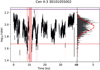 |
Fig. 1 Filtering of Cen X-3 light curves using a log-normal distribution of counts in the 3–70 keV band (see Sect. 3.3). Left panel: light curve since the beginning of observation on 2015 November 30. The pink vertical bands indicate the excluded periods; the horizontal lines indicate the rate limits. Right panel: histogram of counts in logarithmic scale with horizontal lines indicating the adopted limits. We considered as good time intervals those encompassing the ±5σ deviations from the central peak value. |
2.2 Filtering criteria
We filtered out time intervals where the source showed clear eclipses, dips, flares, significant spectral changes, or unusual behavior. To this end, we extracted the source light curves in the 3–7 keV and 7–30 keV energy ranges with 0.1s time bins, and rebinned them to ensure a minimal signal-to-noise ratio (S/N) of 50 eventually taking the largest bin among the two. We defined the hardness ratio for these two bands (hard/soft rates) and studied its variation as a function of time to spot any significant spectral change during our observation. If no major variation is present, we studied the flux variations on the rebinned light curve using the frequency histogram of the total 3–30 keV rates, and excluded the intervals falling at more than 5σ from the Gaussian best-fitting peak, assuming a log-normal distribution. We illustrate our filtering procedure in Fig. 1.
2.3 Pulse search, time-phase matrix, and timing analysis
We barycentered the arrival time of each event in the Solar System frame and performed a Lomb-Scargle (LS) search for coherent signals. We took the highest peak in the LS spectrum as preliminary spin frequency (Pspin), we checked its general consistency with the literature value, and then we refined Pspin using an epoch folding search in a frequency interval around ±5% ×Pspin, after correcting for the binary motion. When available, we used binary orbital parameters from the Fermi-GBM online database2 of XBPs. We report these periods in Table 1.
Adopting this Pspin, we extracted folded pulse profiles in intervals of 1500 s for the whole duration of the observation. We refer to this object, which contains the full set of the time-selected folded profiles, as the time-phase matrix. We calculated each profile S/N according to the standard expression
 (1)
(1)
where pi, σpi, and  are respectively the rate on the i phase bin, its uncertainty, and the average rate of the pulse profile. We rebinned the resulting profiles to obtain a minimum S/N; a value of ~15 was generally satisfactory. Subsequently, we determined the phase of the first harmonic for each of them and plotted their values as a function of time. We checked for the presence of a linear, or quadratic, trend in the phase values (see Fig. 2 for one of the examined sources) through a quadratic least-squares fit of the data. Uncertainties on fit parameters were obtained by bootstraping the time-dependent phases with 1000 realizations. A linear trend would indicate a slightly incorrect pulse period, while a quadratic term would indicate the presence of a significant spin-frequency derivative. To detect such trends, we chose a threshold of 90% significance level on the linear (quadratic) best-fitting coefficients. In the observation of Cen X-3 in particular, we found a significant curvature in the time dependence of the phase, while in all other cases the fit with a constant was always acceptable as no spin–spin derivative was detectable.
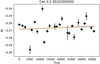 |
Fig. 2 First-harmonic phase of time-resolved pulse profiles extracted along the Cen X-3 observation on 2015 November 30 with time tagged since its start. Pulses are extracted every 1500 s and rebinned to achieve a S/N of 15. The solid line with spread indicates the best linear trend and its 1σ envelope. The phases are obtained by folding the light curve using the period and period derivative shown in Table 1. |
2.4 Energy-phase matrix construction and pulsed fraction
When binary ephemerides are available, we computed the photon arrival time as if they were emitted on the binary system line of nodes. Then, we determined the spin frequency and we accumulated energy-resolved folded profiles using a Nbins value of 32. The energy bin spacing was adjusted to match the FPMA energy resolution (~0.4keV at low energies, 1.2 keV at high energies) in the whole NuSTAR band, resulting in 99 independent bins, in agreement with the response matrix boundaries. Each energy-resolved profile is saved as a row in a phase-energy matrix and stored as a file. We extracted matrices separately for source and background and avoided a direct subtraction to preserve Poissonian statistics. With the same reasoning, it is possible to sum the two FPM units A and B to enhance the signal. We adaptively rebinned the energy scale by requiring that each energy-resolved pulse of the summed source-plus-background matrices had a minimum S/N in each energy-dependent pulse profile. The threshold is optimized to preserve the detection of features in the decaying tail of the spectrum at tens of keV, and for this reason, we started the rebinning computation from the last, highest energy, bin.
From the rebinned matrices, we compute the PF in each energy bin. As described in Appendix A, all integral RMS methods are equivalent, at least for the S/N that we use. We then adopt the FFT method to obtain the harmonic decomposition at the same time:
 (2)
(2)
Here | A0 | is the average value of the pulse profile, which is the zeroth term of the FFT transform, and the terms A1…k are the kth terms of the discrete Fourier transform, so that each | Ak | represents the amplitude of the kth harmonic.
We truncated the Fourier spectral decomposition, using a number of harmonics that describe the pulse with a statistical acceptance level of at least 10%. For Poissonian statistics, Kaastra (2017) gave an approximate recipe for the Cstat to obtain the expected mean and average given the data and model. They showed that under conditions on the total number of counts that are met in our case, the Cstat distribution is Gaussian. In our case, the model is the Fourier decomposition at the nth order. We iterated from a minimum of n = 2 to n = Nbins/2 until the Cstat fell below its expected average plus x times the expected standard deviation, where x is computed for the required significance level (e.g., 1.96 for 10%).
We computed the uncertainty on the PF value using a bootstrap method: for each energy-resolved profile, we simulated 1000 faked profiles assuming Poisson statistics in each phase bin. We computed the average and the standard deviation of the simulated sample, verified that the average is compatible with the value computed from data and used the standard deviation as an estimate of the uncertainty at a 1σ confidence level.
2.5 Harmonic decomposition, lag, and correlation spectra
The pulse profile can be decomposed in Fourier series and, in general, most of the power is in the first two harmonics (known as the fundamental harmonics, or the first harmonic and second harmonic). As these might represent the contribution of different beam patterns (e.g., Tamba et al. 2023), it is informative to investigate their amplitude- and phase-energy dependence separately.
The correlation spectrum is computed taking, for each energy bin, the correlation value between the profile at that energy bin and the full energy-averaged profile subtracted of the contribution of the bin under exam. We computed the discrete cross-correlation function for each energy-resolved bin, as
 (3)
(3)
where  is the correlation value for the kth bin of the pulse profile at energy e, pe is the corresponding pulse profile, and
  is the average pulse profile excluding the one at energy e. Both profiles are normalized to zero average and unitary standard deviation before computing the correlation. However, to determine an informative lag value, instead of taking the highest correlation value from the discrete cross-correlation vector, we model a range of values (seven points) around the peak of the discrete sampling using a constant plus a Gaussian function. The corresponding best-fit Gaussian peak value is taken as the correlation value for that energy bin, and the corresponding peak position is used to derive its lag value in phase units (see Fig. 3 for an illustration).
We computed uncertainties by bootstrapping 100 fake energy-phase matrices using Poissonian statistics and applying the same method to the faked data set. Then, we took the standard deviation of the sample as the 68% confidence interval estimate of the relative quantity. In all cases, we verified that the mean sample value is compatible with the observed value.
By construction, the correlation peaks in the energy range where the statistics are the highest, typically in the 6–10 keV range given the hard spectrum of these sources and the NuSTAR effective area.
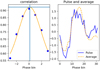 |
Fig. 3 Example of lag and correlation determination for the first energy bin of the Cen X-3 observation (see Sect. 3.3 for details). Left panel: points indicate correlation values as a function of the phase bin. The orange line is the best-fit model. The vertical solid line is drawn at the lag value, while the horizontal solid line is at the correlation value. Right panel: solid blue line is the pulse profile at a given energy; the dashed orange line is the average of all other energy bins. Both profiles are normalized to zero average and unitary standard deviation. |
2.6 Modeling the pulsed fraction spectrum
The method we used to extract and rebin the energy-dependent pulses provides a sensible description of the energy variation of the PF. An immediate consequence of our rebinning is the possibility to evidence the smooth increase from low to high energies in the pulsed signal together with the superimposed deep features corresponding to the ~6.5 keV iron line (EFe) and the cyclotron line (Ecyc). With such an accurate determination of the PF spectrum, we can model the energy dependence in analogy with spectral fitting.
We find evidence for different trends between the low-energy (~2–15 keV) and the high-energy (~ 15–70 keV) bands of the PF. As our focus is on revealing energy-confined features, we model the PF spectrum in two separate energy bands defined by a splitting energy value (Esplit). We search for a convenient Esplit in the range between 10 and 20 keV, which is far from the typical centroid energies of features. For this purpose, we interpolate the PF using a third-order univariate spline from the scipy interpolate package (Virtanen et al. 2020). We compute the spline derivative function and set Esplit equal to the energy corresponding either to a value of zero (i.e., a flex point of the function) or to the first derivative minimum value.
In each segment the increase in the PF with energy varies from source to source and it can be described by a polynomial.
The addition of Gaussian-like absorbing components mimics the sudden decrease in correspondence to the Fe and cyclotron line features. We use a Gaussian initially centered at 6.4 keV for the iron line (EFe), with width σFe = 0.5 keV, while the initial values for the energy (ECyc) and width (σcyc) of cyclotron features are taken from spectral fitting available in the literature. The normalization factors AFe and ACyc are left as free parameters with suitable initial guesses. After allowing for a centroid-energy variation of ±20% and width swings within a few keV, we perform a least-squares fitting. The degree of the polynomial function is chosen adaptively for each source so that the p-value of the best-fit model is above a certain threshold that we set at 5% to trade off between model accuracy and complexity. An additional condition, to prevent overfitting, is that the difference of p-values obtained adding a degree to the polynomial remains above one-fourth of the same threshold.
After performing an initial fit using the lmfit python package (Newville et al. 2023), we explore the parameter distribution and their uncertainties using Markov chain Monte Carlo algorithms from the emcee package (Foreman-Mackey et al. 2013). We use the Goodman & Weare algorithm (Goodman & Weare 2010) with 50 walkers, a burning phase of 500 steps, and a length between 2000 and 5000, to prevent auto-correlation effects. From the sample, we extract the median and 68% percentile as the best parameter estimates. We report for each fit the reduced chi-squared value ( ) and the corresponding degrees of freedom (d.o.f.).
We automated all this process in our dedicated python package. In this way, the same procedure can be straightforwardly applied to the amplitude of any harmonic, being the PF their quadratic sum.
3 Examples of the application of the method
We illustrate our method and the results that can be obtained through some representative NuSTAR observations of prototypical XBP sources listed in Table 1. We used Nbins = 32 and employ the standard FFT RMS method to decompose the signal. Corner plots for the posterior distribution in the parameters of the PF spectrum fit are comprehensively shown in Appendix B.
3.1 4U 1626-67
4U 1626-67 is a persistent ultra-compact low-mass X-ray binary source, whose orbital period is 42 min. The presence of a cyclotron line at ~38 keV is considered a very secure detection, confirmed multiple times with different observatories and spectral models (Orlandini et al. 1998; Coburn et al. 2002; Camero-Arranz et al. 2012). There is also a hint for a second cyclotron harmonic around 60 keV (D’Aì et al. 2017), but to date there has been no other independent confirmirmation. At the time of writing, NuSTAR has observed this source only once for a total exposure of 65.2 ks (in May 2015; ObsID 30101029002).
The PF spectrum in this source shows a significant dynamical range, from ~0.1 at a few keV up to a value close to 1 for the last energy bins. The PF generally increases with energy, but between 5 and 10 keV there is a clear trend reversal, so that the continuum appears to be composed of two broad humps. From a preliminary inspection, we find a local moderately broad feature at the cyclotron line energy, but no clear residual pattern in the iron Kα range.
To best describe the feature at the cyclotron line energy, we should choose an appropriate S/N for the phase-energy matrix. In Fig. 4 we show the PF spectrum for three different choices of S/N (5, 10, and 15, resulting in 85, 71, and 63 independent bins, respectively). Because of the much higher statistics at low energies, this rebinning affects only the high-energy part of the PF spectrum3. There is a good indication that the PF spectrum sharply decreases above 50 keV. Since in this work we are mostly interested in deriving spectral constraints on the cyclotron feature, we looked for a sufficient number of bins to describe the spectral shape without being forced to describe in detail the PF continuum in all the available bands. For this reason, we chose the PF spectrum with a minimum S/N = 10 (which is a good compromise between number of bins and statistics at the cyclotron line), but we removed the last data point in the fitting of the data, as its sharp PF drop would lead to an undesirable higher complexity in the continuum polynomial description.
Given this complex continuum for this source, the fit of the PF was done separately for the soft (2–13 keV) and hard (13–53 keV) X-ray bands. The soft band is well fitted using a fourth-order polynomial ( , for 17 d.o.f.), and no notable local residual is apparent. For the hard band a third-order polynomial is required to achieve a satisfactory fit (
 , for 40 d.o.f.) together with a moderately broad absorption Gaussian close to the cyclotron energy. Panels a and b of Fig. 5 respectively show the data, together with the best-fitting model, and residuals in units of sigma. We show in Table 2 the best-fitting parameters and the line parameters in direct comparison with the spectral fit result from (D’Aì et al. 2017).
The energy cyclotron value and the width between our fitting PF spectrum method and the spectral fit appear to be reasonably close in agreement. The statistical discrepancy, which is a few standard deviations, does not take into account the systematic uncertainty in the spectral estimations from the application of possible different continua as the spectral fit errors are only the statistical uncertainties from a singular adopted continuum model fit. For instance, the cyclotron line width is  keV if the spectral adopted continuum is a power law with a high-energy cutoff (D’Aì et al. 2017), which is fully compatible with the estimate derived from the PF spectrum fit.
There are marginal differences in parameter estimation if the same best fit is considered for the PF spectrum with a lower or higher S/N (e.g., the energy position is 38.0 ± 0.4 keV and 38.6±0.4keV, the line width is 3.9±0.5 and 3.3±0.4 keV for the PF spectrum at S/N = 5 and S/N = 15, respectively).
As shown in panels c and e of Fig. 5, the feature in the PF spectrum at the cyclotron energy is clearly resolved only for the amplitude of the fundamental. Applying the same model used for the PF spectrum, similar values for the cyclotron line energy and width are retrieved (see Table 2), whereas the second harmonic shows a significant lower amplitude and a noisy scatter of data points, which does not permit any firm conclusion; we do not report any fit result in this case.
The correlation spectrum (panel h of Fig. 5) peaks around 10 keV with rapid decrease in the low-energy and the high-energy wings. There is a hint for a small decrease in the correlation value with respect to the adjacent bins at the cyclotron line energy. Similarly, for the same energy bins, in the lag spectrum (panel i of Fig. 5) there is some evidence for an increase in the lag with respect to the adjacent bins. It is clear from the color representation in panel g that the pulse profile has a strong shape discontinuity, which explains these characteristics.
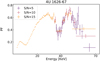 |
Fig. 4 PFFFT obtained with different S/N values for the pulse profile of 4U 1626 – 67. |
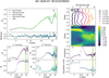 |
Fig. 5 Pulse profile main properties for 4U 1626−67 in ObsID 30101029002. Panel a: pulsed fraction (green points) and its best-fit model (solid lines); the polynomial functions are also shown. Panel b: fit residuals. Panels c−f: phases and amplitudes of the first (A1, ϕ1) and second (A2, ϕ2) harmonics. The vertical colored bands indicate the energy and width of the Gaussian functions fitted to the pulsed fraction. Panel g: selection of normalized pulse profiles at equally logarithmic spaced energies, horizontally shifted for clarity. In each bin the pulse was normalized by subtracting the average and dividing by the standard deviation. Panel h: color-map representation of the normalized pulse profiles as a function of energy. The thin lines represent 20 equally-spaced contours. Panel i: cross-correlation between the pulse profile in each energy band and the average profile. Panel j: corresponding phase lag. The colored vertical bands are the same as in panels d−f. |
Best-fit parameters of the 4U 1626−67 ObsID 30101029002 pulse and amplitude models compared to spectral results.
3.2 Her X-1
Her X-1 is a well-known XBP located at  kpc (Arnason et al. 2021), where a 1.4 M⊙ NS accretes from a low- to intermediate-mass donor star (HZ Her, 1.6–2 M⊙) through Roche-lobe overflow. The NS spins with a period Pspįn = 1.2 s (Giacconi et al. 1971). The orbital period is 1.7 days (Staubert et al. 2007) and also shows superorbital modulation of about 35 d due to the precession of its accretion disk (Brumback et al. 2021; Scott et al. 2000, and references therein).
NuSTAR has observed Her X-1 on multiple occasions. Here we analyze one of the earliest observations performed on 2012 September 22 (ObsID 30002006005) when the count rate was high and stable along the entire observation (see Fürst et al. 2013, for further details). It is known that this prototypical cyclotron line source shows a secular and luminosity-dependent shift in the energy line position (Staubert et al. 2020). As the benchmark for this work, we take as spectral reference the average value (ECyc = 37.5 ± 0.5 keV) obtained from the use of different best-fitting continuum models for this particular ObsID, as found in Fürst et al. (2013); similarly, we take the average value from the best-fitting models for the cyclotron width (σcyc =6.9 ± 1.4 keV). The spectrum of this observation also shows a complex emission pattern of broad iron lines, where the most significant one has a position EFe = 6.55 keV, and a broadness σFe = 0.82 keV. The presence of a second cyclotron harmonic at energies around 70 keV has been sporadically reported (Enoto et al. 2008), but there is no spectral evidence for its presence in this particular data set, given also the limited energy coverage of the FPMs at such energies.
We set the minimum S/N to 16 for the energy-phase matrix, extracted with Nbins= 32, obtaining 74 independent bins. The PF spectrum is split in two separate fits at 11.2 keV. The PF shows a general increasing trend with energy, with two clear Gaussianlike drops at the iron and cyclotron line energies (Fig. 6a)
For the low-energy band a fourth-degree polynomial describes the data very well ( , 10 d.o.f.), together with an absorption Gaussian at energy EFe = 6.50 ± 0.02 keV and σFe = 0.42 ± 0.02 keV. The presence of this feature is statistically very significant (
 for 13 d.o.f., without the line).
For the high-energy band, a third-degree polynomial is needed ( , 47 d.o.f.) for an acceptable fit of the continuum. The feature corresponding to the drop associated with the cyclotron absorption appears smooth and well described using a Gaussian profile. The Gaussian position is 40.44 ± 0.15 keV and σcyc is 6.82 ± 0.19 keV. The cyclotron line position and the width are both roughly consistent with the spectral values, but the feature in the PF spectrum is at slightly higher energy than the corresponding spectral results. In correspondence with the spectral cyclotron position energy (~37 keV, highlighted by the dotted vertical cyan line in panel a of Fig. 6), we note the residuals hinting at the presence of a narrower core, which is within the general structure of the line. This suggests that the PF energy dependence might be more complex than a single structure.
The energy-resolved amplitudes of the first two harmonics closely resemble the PF spectrum (panels c and e of Fig. 6). It is possible in both cases to apply the same model and retrieve the line parameters, which remain consistent with each other (see Table 3 and Fig. 7). In particular, the presence of the iron line feature is much more clearly seen in the fundamental rather than in the second harmonic. We note significant phase drifts at the iron and cyclotron line energies (panels d and f of Fig. 6). While there are no notable features in the correlation spectrum, the lag spectrum shows clear local drops in the feature energies (both for the iron and cyclotron lines) confirming that the full pulse is affected (panels i and j of Fig. 6).
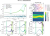 |
Fig. 6 Pulse profile main properties for Her X-1 in ObsID 30002006005. Panel a: pulsed fraction (green points) and its best-fit model (solid lines); polynomial functions are also shown. Panel b: fit residuals. Panels c−f: phases and amplitudes of the first (A1, ϕ1) and second (A2, ϕ2) harmonics. The vertical colored bands indicate the energy and width of the Gaussian functions fitted to the pulsed fraction. Panel g: selection of normalized pulse profiles at equally logarithmic spaced energies, horizontally shifted for clarity. In each bin the pulse was normalized by subtracting the average and dividing by the standard deviation. Panel h: color-map representation of the normalized pulse profiles as a function of energy. The thin lines represent 20 equally-spaced contours. Panel i: cross-correlation between the pulse profile in each energy band and the average profile. Panel j: corresponding phase lag. The colored vertical bands are the same as in panels d−f. |
Her X-1 ObsID 30002006005.
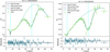 |
Fig. 7 Her X-1 ObsID 30002006005. Shown are data, model, and best-fitting residuals for the fundamental and the second harmonic amplitudes. The dashed blue vertical lines are the initial line fit locations, set at 6.4 keV and 39 keV. |
3.3 Cen X-3
Cen X-3 was the first X-ray pulsar to be recognized as such (Giacconi et al. 1971). Since then, it has been observed with most, if not all, X-ray facilities, becoming a benchmark for theory and observations. The Cen X-3 system is located at  (Arnason et al. 2021) and comprises a O6–8 III donor star, V779 Cen, with a mass of 20.5±0.7 M⊙ (van der Meer et al. 2007) and a radius of 12 R⊙ orbiting in 2.08 d with a neutron star of mass
  spinning at a period of 4.08 s. The X-ray light curve shows eclipses, spanning 20% of the orbital period, due to the high inclination angle (about 70°; Ash et al. 1999).
The accretion flow comes from the donor wind and it is believed to be mediated by an accretion disk (e.g., Suchy et al. 2008). The phase-averaged spectrum of the source can be described by an absorbed Comptonization spectrum with several features. We note a complex of fluorescence lines due to iron (Ebisawa et al. 1996; Iaria et al. 2005) and a cyclotron resonant scattering feature at ~30 keV (Nagase et al. 1992; Santangelo et al. 1998). The overall power law with high-energy cutoff shape of the continuum needs some adjustments like the introduction of a bump around 10 keV (Suchy et al. 2008) or partial covering (Farinelli et al. 2016; Tomar et al. 2021). The pulse profile was decomposed assuming identical beam patter by two poles by Kraus et al. (1996) who find a nonantipodal configuration. This idea has been successfully exploited to interpret the IXPE X-ray polarization results (Tsygankov et al. 2022). NuSTAR observed Cen X-3 from 2015 November 30 to December 1, with an elapsed time of 38.7 ks (ObsID: 30101055002). Different analysis find prominent iron emission around 6.4 keV and cyclotron absorption at about 29 keV, regardless of the specific model or data selection (Tomar et al. 2021; Thalhammer et al. 2021; Tamba et al. 2023).
We determined the spin period after making orbital correction based on the ephemeris by Finger et al. (2010) at 4.80265(2) s, and a spin period derivative ṗ = (3.71 ± 0.15) × 10−9 s s−1, compatible with existing determinations. We extracted the energy phase matrix with 32 Nbins and a minimum S/N = 16. We determined the energy dependent PF and note that typically we can describe the pulse profile using from two to eight harmonics. We truncate our analysis just above 40 keV, as the last energy bin is rather wide and noisy.
As we show in Figs. 8a and b, there is a change in slope between 10 and 20 keV: our algorithm finds a zero derivative at 10.9 keV. Moreover, we see two very pronounced features modeled as Gaussians centered at 6.44 ± 0.02 and 29.8 ± 0.8 keV in addition to a relatively smooth continuum, described by second-order polynomial functions. This is enough to provide a p-value of 1% in the fit. The amplitude of the first and second harmonics (panels c and e in Fig. 8) can be roughly described by the same kind of model. However, the suppression in correspondence of the cyclotron line is not significant for the first harmonic, while the second harmonic shows a much wider feature, suggesting that most of the cyclotron signal is encoded in a structure repeating twice in the pulse profile. The comparison of best-fit parameters for the PF, the first two harmonics, and the literature spectral results are reported in Table 4, showing a solid consistency of the feature centroid energies, while the width of the PF feature is slightly smaller than that in the spectrum. The corner plots in Appendix B confirm the goodness of the PF description. In Figs. 8d and f, we note that the phases of the first harmonic presents some wiggles at the cyclotron energy, a change in trend around 6–7 keV.
To assess the coherence of the pulse profiles along the energy range, we computed the cross-correlation and the lag from aver-age. As shown in Figs. 8h–i, there is a strong dependence of the pulse profile on energy, while the lags start to increase again above the cyclotron energy after showing a plateau between 20 and 30 keV. This is different from the behavior of the phases of the main Fourier components, but the reason is not clear. To have an illustration of the pulse profile energy dependence, we show them as a color map in panel g of Fig. 8, where we can see the gradual phase drift and the change in the pulse shape.
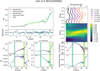 |
Fig. 8 Pulse profile main properties for Cen X-3. Panel a: pulsed fraction (green points) and its best-fit model (solid lines); polynomial functions are also shown. Panel b: fit residuals. Panels c−f: phases and amplitudes of the first (A1, ϕ1) and second (A2, ϕ2) harmonics. The vertical colored bands indicate the energy and width of the Gaussian functions fitted to the pulsed fraction. Panel g: selection of normalized pulse profiles at equally logarithmic spaced energies, horizontally shifted for clarity. In each bin the pulse was normalized by subtracting the average and dividing by the standard deviation. Panel h: color-map representation of the normalized pulse profiles as function of energy. The thin lines represent 20 equally-spaced contours. Panel i: cross-correlation between the pulse profile in each energy band and the average profile. Panel j: corresponding phase lag. The colored vertical bands are the same as in panels d−f. |
Best-fit parameters of the Cen X-3 Obs ID 30101055002 pulse and amplitude models compared to spectral results (Tomar et al. 2021).
3.4 Cepheus X-4
Cepheus X-4 (hereafter Cep X-4) is an accreting X-ray pulsar with spin period of 66.2 s and a Be star as a donor (Ulmer et al. 1973) at a distance of 3.8 ± 0.6 kpc (Bonnet-Bidaud & Mouchet 1998). NuSTAR observed it twice during a bright outburst that occurred in 2014. Here we examine the first observation (ObsID 80002016002), which was performed close to the peak of the outburst. Fürst et al. (2015) analyzed the broadband spectrum, finding a two-component continuum: a soft black-body emission of temperature ~0.9 keV and a power-law emission with a high-energy Fermi-Dirac cutoff. Overimposed on this continuum they found evidence of an iron fluorescence line at energy 6.5 keV, and a cyclotron absorption line at 30.4 ± 0.2 keV with a width of 5.8 ± 0.4 keV. Residuals in the red part of the wing of the cyclotron line required the addition of another Gaussian absorption component at energies of 19.0 ± 0.5 keV and σ = 2.5 ± 0.4 keV. Vybornov et al. (2017) revisited this spectral study, expanding the analysis to include pulse-resolved spectra. This study substantially confirmed the energy position of the iron fluorescence line, the position of the 30 keV cyclotron line, but claimed in addition the detection of a possible harmonic at 54.8 ± 0.5 keV. Differently from the first study, these authors chose to model the residuals in the red wing of the line using an absorption line at ~10 keV. We limit ourselves to the feature at 30 keV.
After the determination of the spin period, Pspin = 66.33568(5) s, we computed the energy phase matrix for different Nbins and minimum S/N and the corresponding spectrum of the PF, choosing a value of 10 to favor the high-energy energy resolution and excluded the last energy bin, which was too noisy. As seen in Figs. 9a and b, the PF increases smoothly from 3 to 20 keV, starting from 0.25 up to a maximum of about 0.4 with a clear drop at about 6.5 keV. The PF trend changes dramatically beyond 20 keV, with a well-defined and deep decrease at ECyc followed by a sharp increase up to values 0.6–0.7 and above.
As reported in Table 5, a polynomial of third degree is necessary to obtain a p-value greater than 0.05 in the PF model in both energy bands, at the splitting energy Esplit= 13.35 keV. The best-fitting value for ECyc is 31.00 ± 0.18 keV, which is ≈ 1 keV higher than the values reported by Fürst et al. (2015) for the same observation, while the cyclotron width is a close match. The position and width of the iron line are consistent with the spectral results.
In panels c and e of Fig. 9, we show the energy dependence of the first and second harmonic amplitudes. The first harmonic clearly shows a drop at ECyc, even if its relative position appears lower with respect to the PF spectrum, while there is a significant difference in the width. The feature in the second harmonic amplitude looks narrow and bound between two apparent peaks, the higher of which has low significance. Given the relatively low signal, our modeling with a polynomial and Gaussian introduces a degeneracy between the functions, preventing us from performing a meaningful parameter determination.
Interestingly, the behavior of the phases for the second harmonic seems to describe a broader shape analogous to the PF. The iron line is clearly evident in the second harmonic rather than in the fundamental harmonic. The lag spectrum reveals a drop at ECyc, which appears very similar to the drop observed in the PF spectrum, whereas the correlation values show a more structured complex, with a sharp discontinuity in the right wing of the cyclotron line, reflecting a change in shape in the pulse.
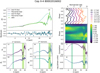 |
Fig. 9 Pulse profile main properties for Cep X-4. Panel a: pulsed fraction (green points) and its best-fit model (solid lines); polynomial functions are also shown. Panel b: fit residuals. Panels c–f: phases and amplitudes of the first (A1, ϕ1) and second (A2, ϕ2) harmonics. The vertical colored bands indicate the energy and width of the Gaussian functions fitted to the pulsed fraction. Panel g: selection of normalized pulse profiles at equally logarithmic spaced energies, horizontally shifted for clarity. In each bin the pulse was normalized by subtracting the average and dividing by the standard deviation. Panel h: color-map representation of the normalized pulse profiles as function of energy. The thin lines represent 20 equally-spaced contours. Panel i: cross-correlation between the pulse profile in each energy band and the average profile. Panel j: corresponding phase lag. The colored vertical bands the same as in panels d–f. |
Best-fit parameters of the Cep X-4 Obs ID 80002016002 pulse and amplitude models compared to spectral results (Fürst et al. 2015).
4 Discussion
We explored various methods for reducing, encoding, and visualizing the information contained in the energy- and phase-dependent pulsed emission of classical X-ray binary pulsars. The aim of this work is to illustrate the general methodology, where we have mainly focused on one particular aspect, the ways that we can exploit the energy-dependent pulse information, particularly the PF spectrum, to investigate the presence and characteristics of features in the energy spectrum. As noted in Sect. 1, it has long been known that the pulse profile changes in connection to some characteristic spectral features, such as the cyclotron line, where it was easy to note clear drops in the PF quantity, when represented in appropriate energy bins. We considered if, and to what extent, it is possible to evolve from a qualitative assessment on the generic scatter plot of PF points versus energy, to physical quantitative estimates of the main parameters responsible for such pulse changes. We analyzed different operative definitions of PF and chose one that was able to best capture the fast variations of the pulse shape at the line energy (see details of this work in Appendix A) and we finely tuned the construction of the energy-phase matrix. A base matrix is originally created according to the instrument energy resolution, but as the typical spectra of XBP show exponential decay, the high-energy part is mostly very noisy. We found that an opportune rebinning, keeping the S/N above a certain threshold, eliminates the intrinsic statistical noise, still preserving the general aspect of the PF spectrum. There is a marginal dependence of the PF spectrum on the number of phase bins and the minimum S/N, so that the matrix construction has, at the end, a few user-defined parameters. However, the choice of the final setup does not affect substantially the parameter determination, as long as the user has a focus on the description of the PF changes at the line energies. We clearly show this via some examples (see Figs. 4 and A.4).
We approached the description of the PF spectrum in purely phenomenological terms. We used a polynomial function, keeping its degree free to vary according to the PF complexity of each source or observation to model data points; the advantages of this choice are that this continuum does not make any assumptions on the physics of a particular source; its terms are uncorrelated orthogonal functions; and it is easy and fast to add higher terms, which keeps a good control of the statistical significance for the addition of each new term. We note that, to our knowledge, there is still no physical procedure to predetermine how the PF behaves in correlation with energy, even for a source whose physical characteristics are already well determined.
Such a simple continuum is, however, unable to fully capture the PF behavior along the whole NuSTAR energy band for PF spectra dominated by high statistics, if we require a reasonably low polynomial degree, as the values of data points are so well determined that the function has to closely pass through them to achieve an acceptable fit. There is a subtle modeling problem: any drop in the PF spectrum could be described with a continuum polynomial, if its degree were sufficiently high. However, it is a scientist’s choice to distinguish the part of the continuum and the locus of line-like features to be modeled differently. The same issue affects spectral analysis in which cyclotron features can sometimes be model-dependent, and their detection significance varies according to the chosen continuum. For this work, we show our method starting from a small sample of sources, where the spectral features (both iron and cyclotron lines) have been assessed multiple times by different authors and instruments, in order to make these features robust benchmarks of our method. Because we knew the exact positions of the features, we found it appropriate to split the data fitting into a low-energy (generally 2–15 keV) and a high-energy (15–70 keV) band. At the moment, the purpose of this division is to reduce the complexity of the fit and better constrain local parameters, but we note that for the case of the double-humped PF continuum of 4U 1626–67 (panel g of Fig. 5), this might suggest a change in the observed emitting regions or in the superposition of different spectral components peaking in different energy bands (see also Tsygankov et al. 2021).
By examining this small sample of XBPs, we note that local PF drops in the spectrum are present at the inferred cyclotron and iron line energies in all cases. These drops are well described with Gaussian profiles. This is a first important point that has emerged from our study. Spectral fits of cyclotron lines use either Gaussian or Lorentzian profiles; it is believed that lines might also hide much more complexity as features are formed not in a single slab, but likely along a geometrical extended environment with different physical conditions (e.g., Schönherr et al. 2007), the superposition of which might skew the profile or make it much more structured. In the case of the examined PF spectra, we only found a hint of a possible more complex structure of the PF at the cyclotron line energy for Her X-1 (Sect. 3.2).
The Fourier spectral decomposition allowed us to test the presence and strength of the features, also for single harmonics. In this work we examined the contributions to the total PF from the fundamental and second harmonic, by taking their energy-dependent amplitude variations. In all cases we find, as expected, that the fundamental amplitude closely reproduces the drop in the PF spectrum at the same energies, whereas for the second harmonic amplitude, for weaker sources like 4U 1626−67 and Cep X 4, there is a noisy scatter that prevents us from deriving meaningful constraints. By directly comparing the PF best-fit model parameters with the values obtained from spectral modeling already present in the literature, two aspects appear remarkable to us: the general consistency of the line positions and widths of the features, with a scatter of a few percent from the corresponding spectral parameters values, and the relative error on the determination of such quantities, which is comparable to the spectral uncertainties. This makes the direct modeling of PF spectra a viable and very sensitive probe of the same spectral features.
In the low-energy band, all four examined sources show emission lines from neutral or ionized Fe Kα lines in the energy spectrum, though not all at the same strength. These emission lines are most likely produced in the pulsar external magnetosphere, either in a truncated accretion disk or by the hot wind of the companion star, or from the accretion stream between the pulsar and the companion. In any of these regions, these fluorescence photons are not clocked with the pulse spin, so that it is expected that their contribution to the PF spectrum mimics an absorption feature, whose amplitude and position must be closely linked to the spectral feature parameters. The very broad and luminous iron line in the Her X-1 system, is indeed prominent in the PF spectrum. The line position closely matches the position of the spectral line peak, whereas the line width appears smaller by a factor of ~2. This is most likely due to the very complex pattern of lines, not just a single one, that is present in this source (Kosec et al. 2022). The NuSTAR spectral resolution does not permit a clear spectroscopic investigations, and disentangling the line contributions over the continuum might easily lead to over- or underestimating the physical parameters in the spectral fit.
For the cases of Cep X-4 and Cen X-3 iron lines, the PF corresponding lines match very well with the spectral results. For 4U 1626−67, the PF spectrum is likely not of sufficient statistical quality to detect this feature; in fact, the line might be intrinsically narrow, with a very low equivalent width compared with the other sources (just few tens of eV; see Koliopanos et al. 2017), so the lack of detection is not surprising. A more in-depth study of the connections between the iron line intensity and the determination of the drop in amplitude in the PF spectra are deferred to a future work.
In addition to the energy-dependent Fourier amplitudes and its integral quantity, the PF, other tools are available from the study of the pulse profiles that rely on how the peaks move in the phase space. The correlation and lag spectra offer an interesting window to spot sudden changes occurring at the feature energy. Changes in the lag spectrum are theoretically expected (Schönherr et al. 2014), and the observations of Her X-1 and Cep X-4 show a lag spectrum with a clear drop in the lag value at energies close to ECyc; however, the observation of 4U 1626−67 indicates an increase in the lag value, whereas no notable change with respect to the overall trend is apparent in Cen X-3. Investigating the physical reasons of such results in the context of this small sample of observations is beyond the scope of the present paper; it will be addressed in a future work compiling results of all cyclotron line sources detected by NuSTAR. Similarly, the correlation spectra are worth a dedicate study; although no clear change in the correlation values are spotted at the line positions, the overall trends contain remarkable information, likely connected with continuum variations (e.g., the correlation values are much more constrained in a narrow range at 10–15% of the maximum value, with the notable exception of the 4U 1626−67 observation, which shows fast and steep decline toward values of ~0.4 at the energy extremes).
Finally, the energy-resolved pulse color-maps offer a rapid and immediate visualization of the peaks’ multiplicity and their strength, which provides a rapid inspection of the actual pulse behavior.
5 Conclusions
We presented a quantitative approach to determining the presence and characteristics of spectral features in the pulse-profile spectra of XRPs. We applied our methodology to a small sample of sources to test its efficacy in comparison to spectral modeling results. Our findings offer strong indications about the consistency and robustness of the method, though a much larger sample of observations, spanning different accretion conditions, need to be explored to conclude whether this method can be straightforwardly used to assess the presence and shape of cyclotron features in other sources, where spectral detection is either lacking or poorly determined. At the moment, this method could be used as a practical toolbox to accompany the spectral analysis, but a clear understanding of the physical mechanisms that produce the PF energy dependence and in general the pulse shape would likely raise it to an independent probe of physical measurement of XBPs spectral features. We aim to extend this study to the full sample of cyclotron line sources observed by NuSTAR to evidence characteristic patterns. We then plan to provide the elaborated data sets together with the methods employed in this paper on a dedicated service where the various energy phases matrices can be re-used4.
Acknowledgements
The research leading to these results has received funding from the European Union’s Horizon 2020 Programme under the AHEAD2020 project (grant agreement no. 871158). E.A., A.D. acknowledge funding from the Italian Space Agency, contract ASI/INAF no. I/004/11/4. We made use of Heasoft and NASA archives for the NuSTAR data. We developed our own timing code for the epoch folding, orbital correction, building of time-phase and energy-phase matrices. This code is based partly on available Python packages such as: astropy (Astropy Collaboration 2013, 2018, 2022), lmfit (Newville et al. 2023), matplotlib (Hunter 2007), emcee (Foreman-Mackey et al. 2013), stingray (Bachetti et al. 2022), corner (Foreman-Mackey 2016), scipy (Virtanen et al. 2020). An online service that reproduces our current results is available on the Renku-lab platform of the Swiss Science Data Centre at https://renkulab.io/projects/carlo.ferrigno/ppanda-light/sessions/new?autostart=1. We are grateful to Dr. P. Kretschmar and Dr. G. Cusumano for precious suggestions on this manuscript, and to the language editor for a careful correction. All remaining issues are our responsibility.
Appendix A Pulsed fraction
We briefly review and discuss here the most commonly used definitions of pulsed fraction (PF) present in the literature.
Because of its simple and straightforward calculation, one of the most commonly used definition of PF is the so-called PFminmax, defined as
 (A.1)
(A.1)
where pmin and pmax are respectively the minimum and the maximum values of the rate in the phase bins array (as shown in Fig. A.1). The PFminmax is strongly biased on how much these values might change with the number of phase bins of the profile, and because the computation is based only on two single reference values of the PF, it is not sensitive to the full integral profile shape.
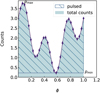 |
Fig. A.1 Generic pulse profile. |
Another operational definition of PF is called area PF (PFarea)
 (A.2)
(A.2)
where N is the number of phase bins and pmin is the minimum of the counts in the profile. This definition directly represents the fraction of pulsed photons with respect to the total emission, though it reduces the complexity of a profile to only one scalar value. As shown in An et al. (2015), this definition is in general affected by a larger uncertainty and potential bias when the minimum of the PF is to be determined in a noisy profile at low statistics.
Finally, the root mean square PF (PFrms) measures the deviation of the pulse from its mean value. The power of this method resides in the possibility to consider the complexity even of noisy pulse profiles. The PFrms can be obtained directly from the root mean square of the array of the pi values, and we call this method PFrms,c, and through the power of Fourier coefficients. It can be obtained as (Dhillon et al. 2009)
![$P{F_{{\rm{rms,c}}}} = {{\sqrt {\sum\nolimits_{i = 0}^N {\,{{\left[ {{{\left( {{p_i} - \bar p} \right)}^2} - \sigma _{{p_i}}^2} \right]} \mathord{\left/ {\vphantom {{\left[ {{{\left( {{p_i} - \bar p} \right)}^2} - \sigma _{{p_i}}^2} \right]} N}} \right. \kern-\nulldelimiterspace} N}} } } \over {\bar p}},$](/articles/aa/full_html/2023/09/aa47062-23/aa47062-23-eq64.png) (A.3)
(A.3)
where  is the average count rate, pi the pulse profile, and
  its uncertainty.
We analyzed two methods for the determination of PF through Fourier decomposition. The most widely used (see An et al. 2015, and references therein) is corrected for the intrinsic variance of the profile, which we call PFFFT,var
 (A.4)
(A.4)
where Nharm is the number of harmonics used to describe the pulse profile, ak and bk are the Fourier coefficients, and  and
and  their variances.5
Alternatively, we measured the rms variability through the direct computation of the Fourier decomposition using an FFT algorithm (see Eq. (2) in Sect. 2.4).
To avoid including white noise, we limited ourselves to a number of harmonics Nharm so that the profile is described at better than 90% confidence level using the goodness of fit derived for Poissonian statistics by Kaastra (2017; see Sect. 2.4).
Figure A.2 shows the spectrum of the PF for Cep X-4 (left) and Her X–1 (right) computed for the different definitions given above (Eq. A.1–2). All the rms-like methods are equivalent, while the PFminmax and the PFarea suffer from uncertainties and bias, especially at higher energies where the statistics of the profiles are poorer.
Despite the global scaling factor among the different methods, rms methods appear more sensitive in describing the overall trend of the PF, and do not severely suffer from poor statistics biases, as shown in the lower panels of Fig. A.2, where we show the relative uncertainty (σPF/PF) for each method. The rms-like methods, therefore, better suit the purpose of understanding the PF energy spectra that show local structures associated with those obtained with spectral analysis. We can choose any of the RMS methods, as the difference is well within the statistical uncertainties and never exceed 1%. The equivalence of methods implies that the correction or the variance is negligible, at least once the pulse profiles have the minimum S/N that we adopt.
These methods are robust against the number of chosen phase bins if in the range 16 ≤ Nbins ≤ 64 (see Fig. A.3). A low value of Nbins underestimates the PF at low energies where the profiles are more complex. Finally, it should be also noted that the choice of the minimum S/N has an impact on the fitting of the PF spectrum, as can be seen in Fig. A.4.
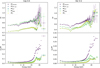 |
Fig. A.2 Comparison of different methods used to obtain the pulsed fraction for Cep X-4 upper left) and Her X-1 ( upper right). In the lower panels the spectra of corresponding relative errors are shown. |
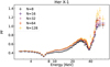 |
Fig. A.3 PFFFT obtained with different Nbins for the pulse profile of Her X–1 analyzed in this work. |
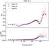 |
Fig. A.4 PFFFT obtained with different S/N values for the pulse profile of Her X–1 analyzed in this work. Nbins = 32. |
Appendix B EMCEE corner plots and fit results
In this Appendix we show the corner plots for the best-fitting values and associated errors of the PF spectra fits presented in Tables 2, 3, 4, and 5.
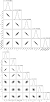 |
Fig. B.1 Corner plots for the 4U 1626−67 PF spectrum fit. The upper and lower panels show the soft and hard band fits, respectively. |
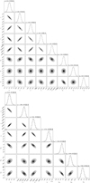 |
Fig. B.2 Corner plots for the Her X-1 pulsed fraction spectrum fit. The upper and lower panels show the soft and hard band fits, respectively. |
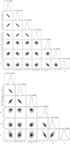 |
Fig. B.3 Corner plots for the Cen X-3 pulsed fraction spectrum fit. The upper and lower panels show the soft and hard band fits, respectively. |
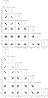 |
Fig. B.4 Corner plots for the Cep X-4 pulsed fraction spectrum fit. The upper and lower panels show the soft and hard band fits, respectively. |
References
- Alonso-Hernández, J., Fürst, F., Kretschmar, P., Caballero, I., & Joyce, A. M. 2022, A&A, 662, A62 [NASA ADS] [CrossRef] [EDP Sciences] [Google Scholar]
- An, H., Archibald, R. F., Hascoët, R., et al. 2015, ApJ, 807, 93 [NASA ADS] [CrossRef] [Google Scholar]
- Arnason, R. M., Papei, H., Barmby, P., Bahramian, A., & Gorski, M. D. 2021, MNRAS, 502, 5455 [NASA ADS] [CrossRef] [Google Scholar]
- Ash, T. D. C., Reynolds, A. P., Roche, P., et al. 1999, MNRAS, 307, 357 [NASA ADS] [CrossRef] [Google Scholar]
- Astropy Collaboration (Robitaille, T. P., et al.) 2013, A&A, 558, A33 [NASA ADS] [CrossRef] [EDP Sciences] [Google Scholar]
- Astropy Collaboration (Price-Whelan, A. M., et al.) 2018, AJ, 156, 123 [Google Scholar]
- Astropy Collaboration (Price-Whelan, A. M., et al.) 2022, ApJ, 935, 167 [NASA ADS] [CrossRef] [Google Scholar]
- Bachetti, M., Huppenkothen, D., Khan, U., et al. 2022, https://zenodo.org/record/7135161 [Google Scholar]
- Basko, M. M., & Sunyaev, R. A. 1976, MNRAS, 175, 395 [Google Scholar]
- Becker, P. A., & Wolff, M. T. 2022, ApJ, 939, 67 [NASA ADS] [CrossRef] [Google Scholar]
- Bonnet-Bidaud, J. M., & Mouchet, M. 1998, A&A, 332, L9 [NASA ADS] [Google Scholar]
- Brumback, M. C., Hickox, R. C., Fürst, F. S., et al. 2021, ApJ, 909, 186 [NASA ADS] [CrossRef] [Google Scholar]
- Camero-Arranz, A., Finger, M. H., Wilson-Hodge, C. A., et al. 2012, ApJ, 754, 20 [NASA ADS] [CrossRef] [Google Scholar]
- Coburn, W., Heindl, W. A., Rothschild, R. E., et al. 2002, ApJ, 580, 394 [NASA ADS] [CrossRef] [Google Scholar]
- D’Aì, A., Cusumano, G., Del Santo, M., La Parola, V., & Segreto, A. 2017, MNRAS, 470, 2457 [CrossRef] [Google Scholar]
- Dhillon, V. S., Marsh, T. R., Littlefair, S. P., et al. 2009, MNRAS, 394, L112 [NASA ADS] [CrossRef] [Google Scholar]
- Ebisawa, K., Day, C. S. R., Kallman, T. R., et al. 1996, PASJ, 48, 425 [NASA ADS] [Google Scholar]
- Enoto, T., Makishima, K., Terada, Y., et al. 2008, PASJ, 60, S57 [NASA ADS] [CrossRef] [Google Scholar]
- Falkner, S. 2018, PhD thesis, Friedrich-Alexander-Universität Erlangen-Nürnberg, Germany [Google Scholar]
- Farinelli, R., Ferrigno, C., Bozzo, E., & Becker, P. A. 2016, A&A, 591, A29 [NASA ADS] [CrossRef] [EDP Sciences] [Google Scholar]
- Ferrigno, C., Becker, P. A., Segreto, A., Mineo, T., & Santangelo, A. 2009, A&A, 498, 825 [NASA ADS] [CrossRef] [EDP Sciences] [Google Scholar]
- Ferrigno, C., Bozzo, E., Falanga, M., et al. 2011a, A&A, 525, A48 [NASA ADS] [CrossRef] [EDP Sciences] [Google Scholar]
- Ferrigno, C., Falanga, M., Bozzo, E., et al. 2011b, A&A, 532, A76 [CrossRef] [EDP Sciences] [Google Scholar]
- Finger, M. H., Wilson-Hodge, C., Camero-Arranz, A., & Jenke, P. 2010, AAS/High Energy Astrophysics Division, 11, 42.08 [NASA ADS] [Google Scholar]
- Foreman-Mackey, D. 2016, J. Open Source Softw., 1, 24 [Google Scholar]
- Foreman-Mackey, D., Hogg, D. W., Lang, D., & Goodman, J. 2013, PASP, 125, 306 [Google Scholar]
- Fürst, F., Grefenstette, B. W., Staubert, R., et al. 2013, ApJ, 779, 69 [CrossRef] [Google Scholar]
- Fürst, F., Pottschmidt, K., Miyasaka, H., et al. 2015, ApJ, 806, L24 [CrossRef] [Google Scholar]
- Ghising, M., Tobrej, M., Rai, B., Tamang, R., & Paul, B. C. 2022, MNRAS, 517, 4132 [NASA ADS] [CrossRef] [Google Scholar]
- Giacconi, R., Gursky, H., Kellogg, E., Schreier, E., & Tananbaum, H. 1971, ApJ, 167, L67 [NASA ADS] [CrossRef] [Google Scholar]
- Goodman, J., & Weare, J. 2010, Commun. Appl. Math. Comput. Sci., 5, 65 [Google Scholar]
- Harrison, F. A., Craig, W. W., Christensen, F. E., et al. 2013, ApJ, 770, 103 [Google Scholar]
- Hunter, J. D. 2007, Comput. Sci. Eng., 9, 90 [NASA ADS] [CrossRef] [Google Scholar]
- Iaria, R., Di Salvo, T., Robba, N. R., et al. 2005, ApJ, 634, L161 [NASA ADS] [CrossRef] [Google Scholar]
- Kaastra, J. S. 2017, A&A, 605, A51 [NASA ADS] [CrossRef] [EDP Sciences] [Google Scholar]
- Koliopanos, F., Vasilopoulos, G., Godet, O., et al. 2017, A&A, 608, A47 [NASA ADS] [CrossRef] [EDP Sciences] [Google Scholar]
- Kosec, P., Kara, E., Fabian, A. C., et al. 2022, ApJ, 936, 185 [NASA ADS] [CrossRef] [Google Scholar]
- Kraus, U., Nollert, H. P., Ruder, H., & Riffert, H. 1995, ApJ, 450, 763 [NASA ADS] [CrossRef] [Google Scholar]
- Kraus, U., Blum, S., Schulte, J., Ruder, H., & Meszaros, P. 1996, ApJ, 467, 794 [NASA ADS] [CrossRef] [Google Scholar]
- Kraus, U., Zahn, C., Weth, C., & Ruder, H. 2003, ApJ, 590, 424 [NASA ADS] [CrossRef] [Google Scholar]
- Lutovinov, A. A., & Tsygankov, S. S. 2009, Astron. Lett., 35, 433 [NASA ADS] [CrossRef] [Google Scholar]
- Meszaros, P. 1992, High-energy radiation from magnetized neutron stars (The University of Chicago Press) [Google Scholar]
- Meszaros, P., & Nagel, W. 1985, ApJ, 299, 138 [NASA ADS] [CrossRef] [Google Scholar]
- Nagel, W. 1981, ApJ, 251, 278 [NASA ADS] [CrossRef] [Google Scholar]
- Nagase, F., Corbet, R. H. D., Day, C. S. R., et al. 1992, ApJ, 396, 147 [NASA ADS] [CrossRef] [Google Scholar]
- Newville, M., Otten, R., Nelson, A., et al. 2023, https://zenodo.org/record/7887568 [Google Scholar]
- Nollert, H. P., Kraus, U., Rebetzky, A., et al. 1989, ESA SP, 1, 551 [NASA ADS] [Google Scholar]
- Orlandini, M., Dal Fiume, D., Frontera, F., et al. 1998, ApJ, 500, L163 [NASA ADS] [CrossRef] [Google Scholar]
- Salganik, A., Tsygankov, S. S., Djupvik, A. A., et al. 2022, MNRAS, 509, 5955 [Google Scholar]
- Santangelo, A., Cusumano, G., dal Fiume, D., et al. 1998, A&A, 338, L59 [NASA ADS] [Google Scholar]
- Schönherr, G., Wilms, J., Kretschmar, P., et al. 2007, A&A, 472, 353 [NASA ADS] [CrossRef] [EDP Sciences] [Google Scholar]
- Schönherr, G., Schwarm, F. W., Falkner, S., et al. 2014, A&A, 564, A8 [NASA ADS] [CrossRef] [EDP Sciences] [Google Scholar]
- Scott, D. M., Leahy, D. A., & Wilson, R. B. 2000, ApJ, 539, 392 [NASA ADS] [CrossRef] [Google Scholar]
- Staubert, R., Shakura, N. I., Postnov, K., et al. 2007, A&A, 465, L25 [NASA ADS] [CrossRef] [EDP Sciences] [Google Scholar]
- Staubert, R., Ducci, L., Ji, L., et al. 2020, A&A, 642, A196 [NASA ADS] [CrossRef] [EDP Sciences] [Google Scholar]
- Suchy, S., Pottschmidt, K., Wilms, J., et al. 2008, ApJ, 675, 1487 [NASA ADS] [CrossRef] [Google Scholar]
- Tamba, T., Odaka, H., Tanimoto, A., et al. 2023, ApJ, 944, 9 [NASA ADS] [CrossRef] [Google Scholar]
- Thalhammer, P., Bissinger, M., Ballhausen, R., et al. 2021, A&A, 656, A105 [NASA ADS] [CrossRef] [EDP Sciences] [Google Scholar]
- Tobrej, M., Rai, B., Ghising, M., Tamang, R., & Paul, B. C. 2023, MNRAS, 518, 4861 [Google Scholar]
- Tomar, G., Pradhan, P., & Paul, B. 2021, MNRAS, 500, 3454 [Google Scholar]
- Tsygankov, S. S., Lutovinov, A. A., Churazov, E. M., & Sunyaev, R. A. 2006, MNRAS, 371, 19 [NASA ADS] [CrossRef] [Google Scholar]
- Tsygankov, S. S., Lutovinov, A. A., Churazov, E. M., & Sunyaev, R. A. 2007, Astron. Lett., 33, 368 [NASA ADS] [CrossRef] [Google Scholar]
- Tsygankov, S. S., Lutovinov, A. A., Molkov, S. V., et al. 2021, ApJ, 909, 154 [NASA ADS] [CrossRef] [Google Scholar]
- Tsygankov, S. S., Molkov, S. V., Doroshenko, V., et al. 2022, A&A, 661, A45 [NASA ADS] [CrossRef] [EDP Sciences] [Google Scholar]
- Ulmer, M. P., Baity, W. A., Wheaton, W. A., & Peterson, L. E. 1973, ApJ, 184, L117 [NASA ADS] [CrossRef] [Google Scholar]
- van der Meer, A., Kaper, L., van Kerkwijk, M. H., Heemskerk, M. H. M., & van den Heuvel, E. P. J. 2007, A&A, 473, 523 [NASA ADS] [CrossRef] [EDP Sciences] [Google Scholar]
- Virtanen, P., Gommers, R., Oliphant, T. E., et al. 2020, Nat. Methods, 17, 261 [Google Scholar]
- Vybornov, V., Klochkov, D., Gornostaev, M., et al. 2017, A&A, 601, A126 [NASA ADS] [CrossRef] [EDP Sciences] [Google Scholar]
- Wang, Y. M., & Welter, G. L. 1981, A&A, 102, 97 [NASA ADS] [Google Scholar]
- Wang, P. J., Kong, L. D., Zhang, S., et al. 2022, ApJ, 935, 125 [NASA ADS] [CrossRef] [Google Scholar]
See the current sample at https://renkulab.io/projects/carlo.ferrigno/ppanda-light/sessions/new?autostart=1


All Tables
Best-fit parameters of the 4U 1626−67 ObsID 30101029002 pulse and amplitude models compared to spectral results.
Best-fit parameters of the Cen X-3 Obs ID 30101055002 pulse and amplitude models compared to spectral results (Tomar et al. 2021).
Best-fit parameters of the Cep X-4 Obs ID 80002016002 pulse and amplitude models compared to spectral results (Fürst et al. 2015).
All Figures
|
Fig. 1 Filtering of Cen X-3 light curves using a log-normal distribution of counts in the 3–70 keV band (see Sect. 3.3). Left panel: light curve since the beginning of observation on 2015 November 30. The pink vertical bands indicate the excluded periods; the horizontal lines indicate the rate limits. Right panel: histogram of counts in logarithmic scale with horizontal lines indicating the adopted limits. We considered as good time intervals those encompassing the ±5σ deviations from the central peak value. |
| In the text | |
|
Fig. 2 First-harmonic phase of time-resolved pulse profiles extracted along the Cen X-3 observation on 2015 November 30 with time tagged since its start. Pulses are extracted every 1500 s and rebinned to achieve a S/N of 15. The solid line with spread indicates the best linear trend and its 1σ envelope. The phases are obtained by folding the light curve using the period and period derivative shown in Table 1. |
| In the text | |
|
Fig. 3 Example of lag and correlation determination for the first energy bin of the Cen X-3 observation (see Sect. 3.3 for details). Left panel: points indicate correlation values as a function of the phase bin. The orange line is the best-fit model. The vertical solid line is drawn at the lag value, while the horizontal solid line is at the correlation value. Right panel: solid blue line is the pulse profile at a given energy; the dashed orange line is the average of all other energy bins. Both profiles are normalized to zero average and unitary standard deviation. |
| In the text | |
|
Fig. 4 PFFFT obtained with different S/N values for the pulse profile of 4U 1626 – 67. |
| In the text | |
|
Fig. 5 Pulse profile main properties for 4U 1626−67 in ObsID 30101029002. Panel a: pulsed fraction (green points) and its best-fit model (solid lines); the polynomial functions are also shown. Panel b: fit residuals. Panels c−f: phases and amplitudes of the first (A1, ϕ1) and second (A2, ϕ2) harmonics. The vertical colored bands indicate the energy and width of the Gaussian functions fitted to the pulsed fraction. Panel g: selection of normalized pulse profiles at equally logarithmic spaced energies, horizontally shifted for clarity. In each bin the pulse was normalized by subtracting the average and dividing by the standard deviation. Panel h: color-map representation of the normalized pulse profiles as a function of energy. The thin lines represent 20 equally-spaced contours. Panel i: cross-correlation between the pulse profile in each energy band and the average profile. Panel j: corresponding phase lag. The colored vertical bands are the same as in panels d−f. |
| In the text | |
|
Fig. 6 Pulse profile main properties for Her X-1 in ObsID 30002006005. Panel a: pulsed fraction (green points) and its best-fit model (solid lines); polynomial functions are also shown. Panel b: fit residuals. Panels c−f: phases and amplitudes of the first (A1, ϕ1) and second (A2, ϕ2) harmonics. The vertical colored bands indicate the energy and width of the Gaussian functions fitted to the pulsed fraction. Panel g: selection of normalized pulse profiles at equally logarithmic spaced energies, horizontally shifted for clarity. In each bin the pulse was normalized by subtracting the average and dividing by the standard deviation. Panel h: color-map representation of the normalized pulse profiles as a function of energy. The thin lines represent 20 equally-spaced contours. Panel i: cross-correlation between the pulse profile in each energy band and the average profile. Panel j: corresponding phase lag. The colored vertical bands are the same as in panels d−f. |
| In the text | |
|
Fig. 7 Her X-1 ObsID 30002006005. Shown are data, model, and best-fitting residuals for the fundamental and the second harmonic amplitudes. The dashed blue vertical lines are the initial line fit locations, set at 6.4 keV and 39 keV. |
| In the text | |
|
Fig. 8 Pulse profile main properties for Cen X-3. Panel a: pulsed fraction (green points) and its best-fit model (solid lines); polynomial functions are also shown. Panel b: fit residuals. Panels c−f: phases and amplitudes of the first (A1, ϕ1) and second (A2, ϕ2) harmonics. The vertical colored bands indicate the energy and width of the Gaussian functions fitted to the pulsed fraction. Panel g: selection of normalized pulse profiles at equally logarithmic spaced energies, horizontally shifted for clarity. In each bin the pulse was normalized by subtracting the average and dividing by the standard deviation. Panel h: color-map representation of the normalized pulse profiles as function of energy. The thin lines represent 20 equally-spaced contours. Panel i: cross-correlation between the pulse profile in each energy band and the average profile. Panel j: corresponding phase lag. The colored vertical bands are the same as in panels d−f. |
| In the text | |
|
Fig. 9 Pulse profile main properties for Cep X-4. Panel a: pulsed fraction (green points) and its best-fit model (solid lines); polynomial functions are also shown. Panel b: fit residuals. Panels c–f: phases and amplitudes of the first (A1, ϕ1) and second (A2, ϕ2) harmonics. The vertical colored bands indicate the energy and width of the Gaussian functions fitted to the pulsed fraction. Panel g: selection of normalized pulse profiles at equally logarithmic spaced energies, horizontally shifted for clarity. In each bin the pulse was normalized by subtracting the average and dividing by the standard deviation. Panel h: color-map representation of the normalized pulse profiles as function of energy. The thin lines represent 20 equally-spaced contours. Panel i: cross-correlation between the pulse profile in each energy band and the average profile. Panel j: corresponding phase lag. The colored vertical bands the same as in panels d–f. |
| In the text | |
|
Fig. A.1 Generic pulse profile. |
| In the text | |
|
Fig. A.2 Comparison of different methods used to obtain the pulsed fraction for Cep X-4 upper left) and Her X-1 ( upper right). In the lower panels the spectra of corresponding relative errors are shown. |
| In the text | |
|
Fig. A.3 PFFFT obtained with different Nbins for the pulse profile of Her X–1 analyzed in this work. |
| In the text | |
|
Fig. A.4 PFFFT obtained with different S/N values for the pulse profile of Her X–1 analyzed in this work. Nbins = 32. |
| In the text | |
|
Fig. B.1 Corner plots for the 4U 1626−67 PF spectrum fit. The upper and lower panels show the soft and hard band fits, respectively. |
| In the text | |
|
Fig. B.2 Corner plots for the Her X-1 pulsed fraction spectrum fit. The upper and lower panels show the soft and hard band fits, respectively. |
| In the text | |
|
Fig. B.3 Corner plots for the Cen X-3 pulsed fraction spectrum fit. The upper and lower panels show the soft and hard band fits, respectively. |
| In the text | |
|
Fig. B.4 Corner plots for the Cep X-4 pulsed fraction spectrum fit. The upper and lower panels show the soft and hard band fits, respectively. |
| In the text | |
Current usage metrics show cumulative count of Article Views (full-text article views including HTML views, PDF and ePub downloads, according to the available data) and Abstracts Views on Vision4Press platform.
Data correspond to usage on the plateform after 2015. The current usage metrics is available 48-96 hours after online publication and is updated daily on week days.
Initial download of the metrics may take a while.