| Issue |
A&A
Volume 576, April 2015
|
|
|---|---|---|
| Article Number | A51 | |
| Number of page(s) | 44 | |
| Section | Extragalactic astronomy | |
| DOI | https://doi.org/10.1051/0004-6361/201425053 | |
| Published online | 26 March 2015 | |
Online material
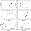 |
Fig. 5
Non-parametric measurements performed in the Lyα images versus the ones performed in the rest-frame UV. From the upperleft to the lowerright: GrP20, M20, CminA, A, S, and SExtractor ellipticity (1 − B/A, where A and B are the semi-major and semi-minor axes of the detection ellipse). The dashed line indicates the 1:1 relation. The numbers reported in each panel correspond to the Spearman test coefficient, r, and probability, p, of uncorrelated datasets. r = 0 indicates no correlation, r = 1(−1) indicates direct(indirect) proportionality. |
| Open with DEXTER | |
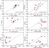 |
Fig. 6
Non-parametric measurements performed in the Lyα images versus the ones performed in the rest-frame optical. From the upper left to the lowerright we show the same parameters as in Fig. 5. |
| Open with DEXTER | |
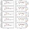 |
Fig. 18
GSB − rP20S vs. M20 measured in the rest-frame optical (left panels) and Lyα (right panel) of the original LARS galaxies (squares). LARS-LAEs are indicated with open circles. In each raw the colour scale corresponds to an integrated physical property derived in Paper II (vertical colour bar). From the top raw the integrated physical properties are stellar mass, Lyα escape fraction, dust-corrected specific star formation rate, nebular reddening, and age. The dashed lines indicate the regions of separation between merging system, normal galaxies, and bulge-dominated systems as presented in Figs. 13 and 14. |
| Open with DEXTER | |
Size of high-z simulated LARS galaxies.
continued.
Morphological parameters of high-z simulated LARS galaxies.
Appendix A: Non-parametric measurements
In this section we explain the way we measured galaxy sizes and non-parametric quantities in detail, and show the results for galaxies with known-profiles.
In Fig. A.1 we summarize the equations adopted in this analysis and first introduced by Conselice et al. (2000) and Lotz et al. (2004).
The code we developed makes a basic use of the ELLIPSE task in iraf.stsdas.isophote and the PHOT task in iraf.digiphot.apphot. We first ran the Source Extractor (SExtractor) software (Bertin & Arnouts 1996) on one galaxy image. This provided the centroid and the elliptical aperture containing the entire galaxy. We adopted configuration parameters like in Bond et al. (2009; DETECT_THRESH = 1.65 and DEBLEND_MINCONT = 1). We followed the choice of DETECT_MINAREA = 30 for the high-z simulations. Those parameters were optimized to provide significant morphological measurements in deep HST-band observations. A larger value of contiguous pixels was adopted to prevent SExtractor from breaking up the clumpy, resolved, original z ~ 0 LARS galaxies into smaller fragments.
We adopted SExtractor centroid, orientation angle, and ellipticity as the fixed ELLIPSE parameters and the SEx AUTO photometry semi-major axis as the reference semi-major axis length (sma0). We then measured flux within ellipses by varying the semi-major axis (sma). The task was able to fit elliptical isophotes at a pre-defined, fixed sma, and works better for well-defined galaxy profiles. As LARS galaxies are irregular, a better convergence of the task was performed by fixing the ellipse orientation and ellipticity.
The ELLIPSE task outputs surface brightness (I(r)) and integrated flux (F) within every sma (ri, ri + 1, ...). We used the given surface brightness to derive the Petrosian ratio (Bershady et al. 2000, η = I(r)/ ⟨ I(r) ⟩) as a function of sma and the integrated flux to estimate r20, r50, r80, the radii containing 20%, 50%, and 80% of the total source flux. The Petrosian semi-major axis (rP20ell) corresponds to the sma where η = 0.2. We defined an elliptical concentration (Cell), proportional to r80/r20. Applying a smoothing kernel with width equal to rP20/5, we also estimated a smoothed-image Petrosian radius (rP20S, Lotz et al. 2004).
The PHOT task outputs fluxes integrated within circular apertures. We derived the corresponding I(r) and estimated the circular Petrosian radius (rP20circ), the circular ![]() , and
, and ![]() . The circular concentration (Ccirc) was then proportional to
. The circular concentration (Ccirc) was then proportional to ![]() /
/![]() .
.
We also defined the signal-to-noise (SN) per pixel as 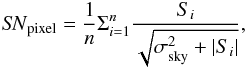 where σsky is the standard deviation of means measured in more than three boxes around the galaxy, Si the signal, and n the number of pixels belonging to a galaxy. The total SN of the galaxy was then obtained by multiplying the SNpixel by
 ![]() . If
. If ![]() ,
,  The asymmetry (A) was calculated as the minimum value of the normalized difference between the galaxy image (I0) and the same one rotated by 180° (I180). We adopted the background (B) correction advised by Conselice et al. (2000) for low SN galaxies. Based on this definition, 0 <A< 1 (e.g., Scarlata et al. 2007; Aguirre et al. 2013; Law et al. 2012). After calculating the position of minimum asymmetry, we ran PHOT on that position and calculated the Petrosian radius (rP20minA),
 ![]() , and
, and ![]() , corresponding to the minimum of asymmetry. The point of the galaxy of minimum asymmetry is generally close to its brightest pixel, but not necessarily to the SExtractor centroid. The concentration (CminA) at minimum asymmetry was then calculated from the
, corresponding to the minimum of asymmetry. The point of the galaxy of minimum asymmetry is generally close to its brightest pixel, but not necessarily to the SExtractor centroid. The concentration (CminA) at minimum asymmetry was then calculated from the ![]() /
/![]() ratio (Conselice et al. 2000; Lotz et al. 2006; Jiang et al. 2013; Holwerda et al. 2014).
ratio (Conselice et al. 2000; Lotz et al. 2006; Jiang et al. 2013; Holwerda et al. 2014).
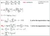 |
Fig. A.1
Basic equations adopted to calculate galaxy size and non-parametric measurements of the LARS original and high-z simulated galaxies. |
| Open with DEXTER | |
Bershady et al. (2000) defined C by measuring photometry inside circular apertures. They estimated that C could be underestimated up to 30%, in the case of an ellipticity of ~ 0.75 and circular aperture, but that it was within 10−15% for early-type galaxies. CminA was the quantity we mainly used throughout the paper.
A galaxy was assumed to be composed of a certain number of pixels, constituting a segmentation map. The non-parametric measurements and SN estimation were performed counting the flux of pixels belonging to that segmentation map. We defined the segmentation map in two ways, one (the fixed-size segmentation map) is an ellipse with sma = rP20 and orientation given by SEx (see Scarlata et al. 2007); one described in Lotz et al. (2004), where the pixels belonging to the segmentation map have surface brightness larger than the value at rP20S. The fixed-size map was mainly concentrated in the central part of the galaxy, the second one could contain bright pixels in the galaxy outskirts.
The Gini coefficient (G) and M20 were also calculated by following the equations in Fig. A.1. Xi (i = 1 to n) correspond to the pixel values, sorted in increasing order, and ![]() the average pixel value, within the chosen segmentation map. fi (i = 1 to n) correspond to the pixel values within the chosen segmentation map, but sorted in decreasing order; xc and yc are the pixels corresponding to SEx centroid. A first value of G (GrP20) was estimated within the first segmentation map (Lotz et al. 2004, 2006; Jiang et al. 2013; Holwerda et al. 2014). A second value (GSB − rP20S) was estimated within the second segmentation map. The latter is sensitive to multiple knots in a galaxy full of structures. Within the fixed-sized segmentation map we measured M20 (Scarlata et al. 2007; Jiang et al. 2013; Aguirre et al. 2013; Holwerda et al. 2014) and S.
the average pixel value, within the chosen segmentation map. fi (i = 1 to n) correspond to the pixel values within the chosen segmentation map, but sorted in decreasing order; xc and yc are the pixels corresponding to SEx centroid. A first value of G (GrP20) was estimated within the first segmentation map (Lotz et al. 2004, 2006; Jiang et al. 2013; Holwerda et al. 2014). A second value (GSB − rP20S) was estimated within the second segmentation map. The latter is sensitive to multiple knots in a galaxy full of structures. Within the fixed-sized segmentation map we measured M20 (Scarlata et al. 2007; Jiang et al. 2013; Aguirre et al. 2013; Holwerda et al. 2014) and S.
The clumpiness (S) was defined by Conselice (2003) as the normalized difference between the galaxy image (I) and the smoothed image (I0.3xrP20, where the smoothing kernel sigma was 0.3 × rP20). The pixels belonging to the galaxy image are the ones within 0.3 and 1.5 times the rP20, i.e. we excluded the very central pixels, which are often unresolved.
We tested our code on the frames showed in Fig. A.2. The code calculations are shown in Fig. A.3. First of all we analytically calculated the theoretical (THEO in the figure) Petrosian ratio and radius of an exponential and de Vaucouleurs profiles. Then, we ran SExtractor and calculated the non-parametric measurements described above.
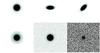 |
Fig. A.2
Simulated profiles used as a test of our code performance. From the upper left to the lower right panels: symmetric exponential profile, exponential profile with ellipticity equal to 0.5 and position angle 0°, exponential profile with ellipticity equal to 0.5 and position angle 45°, de Vaucouleurs profile, asymmetric exponential profile after adding a noise corresponding to a 10σ detection limit 7 times fainter (noise in Tables A.1 and A.2) and 3 times fainter than the fake galaxy flux. They were generated by running the MKOBJECT task in iraf.artdata and noise was added by running the MKNOISE task in iraf.artdata. |
| Open with DEXTER | |
The results are listed in Tables A.1 and A.2. The rP20ell size better recovers the analytical value of an exponential profile. It also well recovers the value in the case of added noise and of a de Vaucouleurs profile. For this reason, we adopted rP20ell as the main size estimator throughout the paper. By comparing with the analytical solution and the estimations by Bershady et al. (2000) and Lotz et al. (2006), we noticed that we could underestimate Ccirc of a de Vaucouleurs profile up to 30%, CminA of an exponential(de Vaucouleurs) profile up to 10(20)%, and overestimate GSB − rP20S up to 10(5)% for an exponential(de Vaucouleurs) profile. M20 is well-recovered for all the profiles within 3%.
Also, we tested our code on the public galaxy stamps from COSMOS and compared the results with the ones obtained with the ZEST software (Scarlata et al. 2007). When assuming the brightest pixel as the centre of a galaxy, we recovered GrP20 values in more than 80% of the cases. As the fixed-size segmentation map is a better choice for redshift comparisons (Scarlata et al. 2007), we tended to prefer GrP20 rather than GSB − rP20S throughout the paper.
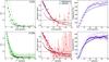 |
Fig. A.3
From the left to the right panels surface brightness, Petrosian ratio, and integrated flux. The upper(lower) row is obtained by using elliptical(circular) aperture and the iraf ELLIPSE(PHOT) task. For an effective radius, Re = 10 pixels, we estimated photometry in the case of a symmetric exponential profile (solid line), exponential profile with ellipticity equal to 0.5 and either position angle 0 (dashed line) or 45 (dotted line) degrees, and of a de Vaucouleurs profile (triangles). The case of adding noise is represented by filled circles with and without errorbars. The analytical Petrosian ratios for exponential (THEOexp) and de Vaucouleurs (THEOdeVauc) profiles are presented in the second-column panels as blue and cyan solid curves respectively. |
| Open with DEXTER | |
Sizes from known profile galaxies of Re = 10 pixels.
Morphology measurements from known profile galaxies of Re = 10 pixels.
Appendix A.1: Comparison between original and simulated galaxy morphological parameters
Following the method described in the previous section, we estimated sizes and morphological parameters in the continuum and line images. We adopted the same method in the case a galaxy was simulated to be at z ~ 2 and observed in different depth surveys. To quantify the morphological parameter variations owing pixel resampling and added noise, we defined Δ(param), 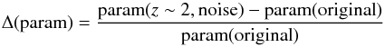 (A.1)which represented the difference between the measurement of a parameter in the simulated and in the original image, normalized to the value in the original image. By definition, Δ(param) tended to be zero when the two measurements were very similar, tended to be equal to −1 when the measurement in the simulated image was much smaller than in the original one, and equal to 1 when the measurement in the simulated image was twice that in the original one. We calculated Δ(param) for every galaxy and estimated the mean and the standard deviation.
In Fig. A.4 we show the results. A, CminA, GrP20, and M20 were all preserved after pixel resampling in the continuum images. Owing survey depth, A decreased.
Huertas-Company et al. (2014) studied the variation of A, G, and M20 due to resampling the rest-frame optical of local galaxies to z> 1. They found that A can increase up to 50%, G up to 10%, while M20 can decrease up to 10%. These trends were observed to be more pronounced for early-type galaxies; Lotz et al. (2006) resampled the rest-frame UV of a few sources from z = 1.5 to z = 4, finding that G and M20 were preserved, consistent with our results. Overzier et al. (2010) investigated the change of A, C, G, and M20 when resampling z = 0.2 Lyman break analogues to z = 2. They gave an R-value scale, where | R| ~ 0 when the difference between the median parameter measured in the resampled and in the original image was small and | R| ~ 1 when was comparable to the sample scatter. They found RA = −1.1, RC = 0.02, RG = −0.34, and RM20 = −0.43 in the rest-frame UV and RA = −0.46, RC = −0.52, RG = −1.1, and RM20 = −0.26 in the rest-frame optical. Recently, Petty et al. (2014) explored the variations of G and M20 of local LIRGS when simulated to be at z = 0.5, 1.5, 2, 3 and in a survey with the HUDF depth. Some of the galaxies in their sample, characterized by clumps and filamentary structures (typical of merging systems) in high-resolution HST images, tended to appear as disk-like galaxies by z = 2. Some others maintained merging systems’ morphology. All these trends are in agreement with our findings, but they also tell us that the variations do not follow a specific trend for irregular galaxies.
In the Lyα images, A tended to decrease and CminA could increase due to pixel resampling. Owing survey depth, all the four parameters tended to decrease and A significantly decreased.
|
Fig. A.4
Mean Δ(param) as defined in Eq. (A.1) vs. simulated survey depth. param is A (upper left), CminA (upper right), GrP20 (lower left), and M20 (lower right) for the rest-frame optical, UV, and Lyα simulated images. The deepest simulated survey is represented by the most right data point in each panel. The error bars represent the standard deviation among all the high-z simulated LARS galaxies. In the case fewer-than-twelve galaxies are detected at a specific depth, the error bars is increased proportionally to the number of undetected galaxies. The numbers on the top right corner of each panel represent the Spearman test coefficient, r, and probability, p, of uncorrelated datasets, assuming that the depth vector indicates the deepest survey on the right of the x-axis. |
|
| Open with DEXTER | |
Another way to study the change of morphological parameters is to look at pairs of them, like GrP20 vs. M20 and A vs. CminA. In Fig. A.5 we show the diagrams of two-parameters, measured in the rest-frame optical, UV, and Lyα images. Our analysis showed that the G and M20 estimations were not
affected by resolution and survey depth. Therefore, they were useful for comparisons at different redshifts and different survey depths throughout the paper.
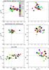 |
Fig. A.5
GrP20 vs. M20 (first column) and A vs. CminA (second column) measured in the rest-frame optical (upper), UV (middle), and Lyα (lower) images. Small and big diamonds with error bars indicate the parameters of the original and (deepest survey) high-z simulated LARS galaxies. The dashed and dotted-dashed lines indicate the separation between merging system and normal galaxies’ parameter space. Owing pixel resampling the galaxies stay in the same region of the GrP20 vs. M20 diagram. |
| Open with DEXTER | |
Appendix B: LARS galaxies simulated at high redshift in a deep and shallow survey
In this appendix, we show the continuum and line maps of the high-z simulated LARS galaxies. Figures B.1−B.3 present
 |
Fig. B.1
Rest-frame UV (first column), Lyα (second column), rest-frame optical (third column), and Hα (fourth column panels) images for z2L01, z2L02, z2L03, z2L05, and z2L07 in the deepest survey, probed here. Every panel is 20 × 17 kpc wide. The reddish ellipses indicate SEx apertures (dashed curves indicate flagged sources according to SEx convention), corresponding to the assumed detection parameters: DETECT THRESH = 1.65, DETECT MINAREA = 30, and DEBLEND MINCONT = 1 from Bond et al. (2009). The colour scaling is logarithmic and chosen to show a visually consistent background noise. |
| Open with DEXTER | |
rest-frame UV, Lyα, rest-frame optical, and Hα images in the deepest survey depth probed here, together with SEx detection apertures. In Figs. B.4−B.6, we show the same stamps but for a shallower simulated survey.
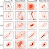 |
Fig. B.2
As Fig. B.1 for z2L08, z2L09, z2L10, z2L11, and z2L12. In the case of z2L09 and z2L11 the size is 27 × 27 kpc and 33 × 30 kpc respectively to fit their elongated shapes. For these galaxies SEx apertures in Lyα happen to be outside the shown region. |
| Open with DEXTER | |
|
Fig. B.3
As Fig. B.1 for z2L13 and z2L14. For z2L13 SEx aperture in Lyα happens to be outside the shown region. Also, two main sources connected by undetectable (mrest − UV> 30 and F(Hα) < 6E-19 erg s-1 cm-2) surface brightness structures are seen in UV continuum and Hα. By using the chosen detection parameters, SEx found two sources as separated. As in Lyα and optical continuum the photometric measurements are done centring the aperture close to the right clump, we locate the aperture on that one for the photometry in UV and Hα as well. |
|
| Open with DEXTER | |
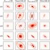 |
Fig. B.4
As B.1, but for a shallow simulated survey. The dashed-line apertures indicate that some detected source is blended to another (Bertin & Arnouts 1996). |
| Open with DEXTER | |
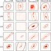 |
Fig. B.5
As Fig. B.2, but for a shallow simulated survey. z2L09 and z2L10 are not detected in Lyα at a 10σ detection limit of 3E-18 erg s-1 cm-2. |
| Open with DEXTER | |
|
Fig. B.6
As Fig. B.3, but for a shallow simulated survey. Only the bright right clump of z2L13 is detected in UV at a 10σ detection limit of mrest − UV = 29. Its Lyα emission is localized around the lower side of the right clump. In Hα the two overlapping sources become well separated. |
|
| Open with DEXTER | |
Appendix C: Surface brightness profiles of original and high-z simulated LARS galaxies
We present here the surface brightness profiles of eleven LARS galaxies studied in this paper. The profiles of L01 were shown
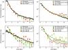 |
Fig. C.1
Normalized surface brightness profiles of L02. Black points with error bars correspond to the surface brightness profile of the original LARS images in the rest-frame UV, optical, and Lyα as explained in the text (Fig. 8). The red squares represent the profile affected by background noise, for a certain shallow survey. |
| Open with DEXTER | |
in Fig. 8. Every figure in this appendix shows four panels, rest-frame UV and optical continua, Lyα and Hα lines. The profiles are normalized to 2 kpc to compare continuum and line profiles.
|
Fig. C.2
Same colour coding as in Fig. C.1, but for z2L03 and z2L05. The deepest and intermediate depth surveys are shown for z2L03(z2L05) in magenta(red) symbols with error bars, as throughout the paper. |
|
| Open with DEXTER | |
|
Fig. C.3
Same colour coding as in Fig. C.1, but for z2L07 and z2L08. The deepest and intermediate depth surveys are shown for z2L07(z2L08) in blue(light green) symbols with error bars. |
|
| Open with DEXTER | |
|
Fig. C.4
Same colour coding as in Fig. C.1, but for z2L09 and z2L10. The deepest and intermediate depth surveys are shown for z2L09(z2L10) in black(dark red) symbols with error bars. |
|
| Open with DEXTER | |
|
Fig. C.5
Same colour coding as in Fig. C.1, but for z2L11 and z2L12. The deepest and intermediate depth surveys are shown for z2L11(z2L12) in dark green(orange) symbols with error bars. |
|
| Open with DEXTER | |
|
Fig. C.6
Same colour coding as in Fig. C.1, but for z2L13 and z2L14. The deepest and intermediate depth surveys are shown for z2L13(z2L14) in grey(pink) symbols with error bars. |
|
| Open with DEXTER | |
© ESO, 2015
Current usage metrics show cumulative count of Article Views (full-text article views including HTML views, PDF and ePub downloads, according to the available data) and Abstracts Views on Vision4Press platform.
Data correspond to usage on the plateform after 2015. The current usage metrics is available 48-96 hours after online publication and is updated daily on week days.
Initial download of the metrics may take a while.