


| Issue |
A&A
Volume 711, July 2026
|
|
|---|---|---|
| Article Number | A173 | |
| Number of page(s) | 21 | |
| Section | Planets, planetary systems, and small bodies | |
| DOI | https://doi.org/10.1051/0004-6361/202659585 | |
| Published online | 13 July 2026 | |
Planetary formation tracks on the Hertzsprung–Russell diagram
Visualising the processes of giant planet growth
1
Division of Space Research & Planetary Sciences, Physics Institute, University of Bern,
Sidlerstr. 5,
3012
Bern,
Switzerland
2
Fakultät für Physik, Universität Duisburg–Essen,
Lotharstr. 1,
47057
Duisburg,
Germany
3
Max-Planck-Institut für Astronomie,
Königstuhl 17,
69117
Heidelberg,
Germany
4
Center for Space and Habitability, University of Bern,
Gesellschaftsstr. 6,
Bern
3012,
Switzerland
★ Corresponding author: This email address is being protected from spambots. You need JavaScript enabled to view it.
Received:
23
February
2026
Accepted:
18
May
2026
Abstract
Context. The Hertzsprung-Russell diagram (HRD) has long served as a cornerstone of astrophysics, illustrating the relationship between stellar luminosity and effective temperature. Although HRDs have been instrumental in understanding stellar evolution, they have rarely been applied to planet formation.
Aims. We extended the HRD framework to visualise planet formation and provide a new perspective on the physical processes involved. Specifically, we investigated how gas and solid accretion, cooling and contraction, and orbital migration shape these tracks under different formation scenarios.
Methods. We used the Bern model to calculate the interior structure of planets throughout their entire formation and evolution. We also coupled this, for the first time, with radiation-hydrodynamical simulations to dynamically calculate the accretion shock heating efficiency, providing insight into the cold-start and hot-start ambiguity.
Results. The planetary HRDs exhibit three branches, each corresponding to a distinct phase of planet formation. The first phase, the ascending branch, is heavily influenced by the size of the smallest accreted bodies, the associated solid accretion rate, and orbital migration. During this phase, the HR tracks rise steeply. For in situ planetesimal accretion, we analytically derive L ∝ T8. The second phase, the planetary horizontal branch, begins when the gas accretion rate becomes disc-limited, and the planet detaches from the disc before contracting rapidly. Planets move nearly horizontally to the left, with hot accretion, more massive planets, and pebble accretion leading to upward bending. Planetary interiors are close to an ideal gas at detachment, but increasing electron degeneracy causes the central temperature to decrease, stabilising the radius and halting the rapid movement to the left. The third phase, the descending branch, begins when the effective temperature begins to decrease. Gas accretion ceases during this phase, and planets join classical constant-mass cooling tracks. Because the radius changes only weakly, the tracks descend diagonally with L ~ T4. We also find substantial agreement between our analysed tracks, synthetic-population data, and observational data.
Conclusions. Planetary HRDs provide a unique way to link the luminosities and effective temperatures of young planets to their formation physics, with pebble and planetesimal accretion producing distinct early-time tracks. Comparisons with currently directly imaged planets are broadly consistent with our tracks because these objects are mostly non-accreting or near the end of their formation and are expected to follow standard post-formation cooling evolution. However, observationally populating the short-lived early horizontal or ascending branch will be challenging, and interpreting embedded, actively accreting planets will require models that include accretion-shock emission and circumplanetary-disc reprocessing.
Key words: planets and satellites: formation / planets and satellites: gaseous planets / planets and satellites: general / Hertzsprung-Russell and C-M diagrams
© The Authors 2026
 Open Access article, published by EDP Sciences, under the terms of the Creative Commons Attribution License (https://creativecommons.org/licenses/by/4.0), which permits unrestricted use, distribution, and reproduction in any medium, provided the original work is properly cited.
This article is published in open access under the Subscribe to Open model. This email address is being protected from spambots. You need JavaScript enabled to view it. to support open access publication.
1 Introduction
The Hertzsprung-Russell diagram (HRD; after Hertzsprung 1909 and Russell 1914) is a fundamental tool in astrophysics, traditionally used to illustrate the relationship between the luminosity of a star and its surface temperature1. This diagram has been instrumental in understanding stellar evolution, mapping the life cycle of stars from their formation to their final stages. It provides insights into key physical processes, including nuclear fusion, interior structure, and energy transport, making it an indispensable framework in the field. However, although the HRD has been extensively used for studying stars, its application to giant planet formation remains largely unexplored.
This paper aims to bridge this gap by employing the HRD to describe and illustrate the formation process from an alternative perspective. Our concept of the planetary HRD is intended to serve as a step towards a basic framework for future classifications of observed young and forming planets. Until recently, no direct observation of the planetary formation process or of these objects existed. However, a new era of observations has recently begun in which such detections, although challenging, have become possible. These detections have opened new avenues for exploring planet formation in unprecedented detail and in a direct way. These observations fall into three different categories: kinematic detections (Pinte et al. 2019, 2020), potential gap planets (Zhang et al. 2018; Lodato et al. 2019; Asensio-Torres et al. 2021; Ruzza et al. 2025), and directly imaged planets.
Among the last category, the first unambiguous direct discoveries of forming planets were PDS70 b (Keppler et al. 2018) and PDS70 c (Haffert et al. 2019), followed more recently by WISPIT 2 b (van Capelleveen et al. 2025; Close et al. 2025) and V2376 Ori b (Vila et al. 2025). The planets are observed at multiple wavelengths, revealing the photosphere (Müller et al. 2018), the gas accretion shock (Wagner et al. 2018; Hashimoto et al. 2020; Zhou et al. 2021), and the circumplanetary disc (Isella et al. 2019; Christiaens et al. 2019; Benisty et al. 2021; Shibaike & Mordasini 2024). These multi-wavelength observations are pivotal for testing and refining theoretical models. Expanding this topic is also essential for current instruments such as SPHERE or ALMA, and for future instruments including RISTRETTO (Lovis et al. 2022, 2024; Blackman et al. 2026), the SPHERE+ project (Boccaletti et al. 2020; Mazoyer et al. 2024), and several instruments at the Extremely Large Telescope (ELT), for example the Mid-infrared ELT Imager and Spectrograph (METIS; Oberg et al. 2023; Feldt et al. 2024; Takami et al. 2025; Marleau et al. 2025).
This work represents a first step towards addressing this challenge by investigating the bolometric luminosity and surface temperature evolution of planets during their formation and evolution.
We used a global, self-consistently coupled model, the Bern model (see the review in Burn & Mordasini 2024), extended by several new elements. Although this approach is an approximation, our low-dimensional 1D model does not suffer from the limitations of 2D and 3D hydrodynamic simulations, which currently can only be run for selected cases and short timescales. Our approach allows us to track long-term evolutionary processes and derive population-level insights, similar to how the stellar HRD enables tracking of certain phases in a star’s life and ultimately links them to its internal physics.
In this paper, we focus on the forming planet itself, by definition of the HRD, and assume spherically symmetric accretion. Other aspects, such as a potential circumplanetary disc, non-spherical gas accretion, and the effects of the surrounding protoplanetary disc and infalling gas on the observability, will be addressed in subsequent works.
This paper is structured as follows. In Sect. 2, we review the main approach for calculating the luminosity L and the surface temperature T. We extend the model to address the cold-hot-start ambiguity arising from gas accretion at the accretion shock using the results of Marleau et al. (2019b), and we describe this extension in Sect. 2.2.4. This approach yields the fraction of accretion luminosity that is wither radiated away or incorporated into the growing planet. In Sect. 3, we describe our nominal initial conditions, which result in an HRD of our so-called default case, and then compare and discuss variations in the setup to understand different processes and explore new parameter spaces. In Sect. 3.6, we introduce a new formation scenario that includes pebbles and the two-population model of Birnstiel et al. (2012). Through these comparisons, we identify trends and features that could form the basis for interpreting future observations. In Sect. 4, we discuss our results, including comparisons with synthetic-population and observational data, and we present our conclusions. Section 5 then summarises our main findings.
2 Model
Emsenhuber et al. (2021) describes the Bern model in detail. In short, the Bern model is a global planet formation and evolution model that includes the calculation of the 1D spherically symmetric interior structure of (proto)planets and is designed to study the formation and long-term evolution of planetary systems. In this work, however, we focus on single-embryo formation scenarios. In this section, we concentrate on relevant model updates and key aspects of the calculation of luminosity and surface temperature, based on Mordasini et al. (2012).
2.1 Envelope structure and luminosity calculation
Compared with Mordasini et al. (2012), the basic 1D envelope structure equations remain unchanged, so we do not repeat them here (see the original work for the derivation and numerical implementation). The only update relevant to this paper is the opacity treatment, where we combine radiative and conductive opacities harmonically, effectively approximating their minimum:
 (1)
(1)
(Kippenhahn et al. 2013; Polman & Mordasini 2024). Here, κrad is the radiative opacity based on the grain opacities of Bell & Lin (1994) and the molecular opacities from Freedman et al. (2008). The conductive opacity κcond follows Cassisi et al. (2007). For κrad, we multiplied the contribution of the interstellar medium grain opacity by a reduction factor of fopa = 0.003 following Mordasini et al. (2014) (see also Ormel 2014). Small grains are introduced into the envelope by accreted gas, but their opacity is reduced through coagulation and settling in planetary atmospheres. The opacity influences the radiative temperature gradient, ∇rad, which is given by
 (2)
(2)
where σ denotes the Stefan–Boltzmann constant, G the gravitational constant, P the pressure, T the temperature, L the luminosity, and m the mass enclosed within the local radius r. The radiative gradient is applied only in radiative regions, which are determined according to the Schwarzschild stability criterion as follows:
 (3)
(3)
where ∇ad is the adiabatic gradient,
 (4)
(4)
Here, S is the entropy, which is used in the convective regions (∇ad < ∇rad) and is obtained directly from the tabulated equation of state of Chabrier & Debras (2021). We use this equation of state throughout, assuming a constant gas mixture with X = 0.76 and Y = 0.24, and no metals (Z = 0).
For the luminosity, L, in radiative regions (Eq. (2)), we adopted the simplification
 (5)
(5)
which formally assumes a constant L throughout the envelope, originating in the core. Although this assumption is not strictly correct, the actual local value of l affects the internal structure only in radiative layers (Eq. (2)) and not in convective regions. In thin outer radiative layers with negligible mass, l = L provides a very good approximation (see Section 3.4 of Mordasini et al. 2012). Berardo & Cumming (2017) find that the inner radiative layers can contain significant mass; however, these layers do not appear for the parameters relevant to our simulations. High gas accretion rates (Ṁg > 10−3 M⊕ yr−1) with high shock temperatures (Tsh > 2500 K) are required to reach the predicted heating regime from Berardo et al. (2017) and to generate deep radiative layers. We do not see this regime in our simulations.
For the total luminosity budget, L = Ltot, we followed total energy conservation, following the approach of Mordasini et al. (2012). This approach inherently accounts for the core luminosity resulting from solid accretion, which dominates during the early formation phase, and for the energy released due to envelope cooling and contraction at constant mass, which is the primary source of luminosity during the evolutionary phase of giant planets. The approach produces long-term cooling tracks at constant mass during the evolutionary phase, in excellent agreement with conventional methods (see e.g. Marleau et al. 2019a). In Ltot, we include the luminosity generated by radiogenic decay (Lradio), which is very small (Mordasini et al. 2012), and from deuterium burning (LD burn) (Mollière & Mordasini 2012). We also considered a potential heating contribution generated at the accretion shock by accreting gas (details in Sect. 2.2.4). Therefore, the total luminosity is
 (6)
(6)
Here, C(LM + LR) is the sum of the luminosity generated by accreting mass, that is, solids and gas (LM = LM,s + LM,g), and from the changing radius R, multiplied by the correction factor C. This correction accounts for neglecting the factor ξ, which represents the internal mass distribution and energy content of the planet (see Mordasini et al. 2012).
The total energy conservation approach of Mordasini et al. (2012) includes the gas accretion luminosity Lacc, max, the maximal shock luminosity associated with detached gas accretion in Ltot, thereby yielding ‘hot starts’ by default, as in Emsenhuber et al. (2021). We therefore introduce the shock-heating efficiency factor k, such that the limiting cases correspond to the classical cold and hot starts,
 (7)
(7)
We discuss the k factor and the cold-hot start paradigm in detail in Sect. 2.2.4.
For the analysis of the results, we also used LM,s, the luminosity due to the accretion of solids. We calculated LM,s by assuming that solids start with zero initial velocity infinitely far from the planet and reach its core. This yields a luminosity
 (8)
(8)
where Mc is the mass of the core, Rc is the radius of the core and Ṁc the rate of solid accretion. We did not use this expression to calculate the total luminosity, because it is already included in Eq. (6), but it is useful to separate contributions to the total luminosity. In reality accreted solids likely dissolve in the gaseous envelope once it becomes sufficiently massive (e.g. Podolak et al. 1988; Helled & Stevenson 2024). However, this effect is not critical for our study, because at that stage the luminosity budget is dominated by gas accretion and the contribution from solid accretion has become negligible.
To analyse and compare the simulations, we also tracked the maximal bolometric luminosity, defined as the sum of the intrinsic luminosity and the remaining luminosity from the accretion:
 (9)
(9)
This corresponds to the luminosity that an observer would measure in the absence of extinction or absorption.
2.2 Boundary conditions
In the core accretion scenario of giant planet formation, planets undergo three distinct phases (Bodenheimer et al. 2000; Mordasini et al. 2012). The initial formation of very low-mass protoplanets begins in the ‘attached’ phase before transitioning to the ‘detached’ phase, during which they accrete most of their mass. The formation process ends in the third phase, the evolutionary phase at constant mass. In each of these distinct phases, a unique set of boundary conditions must be specified to solve the structure equations.
2.2.1 The attached phase
In the attached phase of planet formation, the very young planetary core with relatively low mass is still embedded in the protoplanetary disc. The planet’s envelope is attached to the surrounding nebula, making the boundary between the two indistinguishable from an observational perspective (Ormel et al. 2015). Thus, the boundary condition for the pressure is given by the nebula Pneb, which we assumed to be the disc’s midplane pressure from the disc model (Pollack et al. 1996). The surface temperature, Ts, of the planet is controlled by both the intrinsic temperature,
 (10)
(10)
 (11)
(11)
and the disc midplane temperature, Td, given by the time-dependent disc model. The surface temperature follows the sum of the energy fluxes:
 (12)
(12)
To determine the outer radius of the planet, we considered which part of the surrounding gas is bound to the planet. The relevant radii are the Bondi (or accretion) radius,
 (13)
(13)
where cs is the speed of sound in the surrounding medium, i.e. the disc, and the Hill radius,
 (14)
(14)
where a is the planet’s semi-major axis and M⋆ is the stellar mass. Following Lissauer et al. (2009), the outer radius Rout is
 (15)
(15)
which reduces approximately to the smaller of RB and RH/4 and provides a first-order approximation to account for the fact that gas in the outer parts of the Hill sphere is not bound to the planet but participates in the surrounding flow in the gas disc, as shown by hydrodynamic simulations (e.g. Ormel et al. 2015; Cimerman et al. 2017; Ali-Dib et al. 2020; Moldenhauer et al. 2022). Although more sophisticated approaches exist (Ali-Dib et al. 2020; Bailey & Zhu 2024; Savignac & Lee 2024), we adopted the approximation of Lissauer et al. (2009) for simplicity, because the principle that cooling of the deeper quasi-1D part of the envelope ultimately regulates gas accretion appears robust (Bailey & Zhu 2024).
With five boundary conditions specified for T, P, Rout, Rc and Ltot, we solved the initial structure equations for a unique total planetary mass, Mp, which provides an indirect measure of the gas accretion rate. We iterated on Mp until the correct known inner boundary condition for Mc was satisfied. Details are given in Mordasini et al. (2012).
During the attached phase, the gas accretion rate scales with the envelope’s capacity to radiate away energy and contract, a process known as the Kelvin–Helmholtz timescale (τKH), allowing additional gas to flow in. Thus, the accretion rate is not yet limited by the disc but by the planetary properties. Although several parametrisations for τKH exist in the literature (e.g. Ikoma et al. 2000; Mordasini et al. 2014), we find that directly solving the structure equations is important because it establishes a self-consistent link between solid and gas accretion (Pollack et al. 1996; Kessler & Alibert 2023).
2.2.2 The detached phase
As the core mass increases during the attached phase, the gas accretion rate gradually accelerates. Eventually, the gas accretion rate exceeds the maximum supply capacity of the surrounding disc. At this point, the detached phase (also called the transition stage; Bodenheimer et al. 2000) begins. In this phase, the accretion rates are known because the disc now limits the gas accretion rate. However, in contrast to the attached phase, where we iterated on the mass to determine the gas accretion rate, we instead iterated on the radius, Rp, until we converged on the known total planetary mass, Mp. We adopted the maximum disc-limited gas accretion rate, Ṁgas,max, from Mordasini et al. (2012), based on a Bondi-Hill-limited accretion regime.
Because the planet’s outermost envelope layer is no longer attached to the background nebula, gas free-falls onto the planet, generating additional pressure at the accretion shock in the form of ram pressure,
 (16)
(16)
where we set Ṁgas = Ṁgas, max and vff is the free-fall velocity,
 (17)
(17)
The new boundary condition for the pressure is then given by
 (18)
(18)
where we also accounted for photospheric pressure for material above the τ = 2/3 layer using the Eddington expression, PEdd = 2g/3κ, and the (negligible) radiation pressure, Prad = 2σT4/3c, where c is the speed of light. The surface temperature is again given by Eq. (12). However, since Td ≲ 100 K, Tin quickly becomes dominant in the detached phase, yielding
 (19)
(19)
Here, Tin is calculated from Eq. (10) and therefore includes the contribution from the accretion shock through our definition of Ltot in Eq. (6).
2.2.3 The evolution phase
The final phase begins once the gas disc around the planet disperses, letting it evolve at a constant mass. The cessation of gas accretion also implies that there is no resupply of grains (Mordasini et al. 2014). Consequently, we gradually reduced fopa to 0 once Ṁgas ≤ 10−5 M⊕ yr−1. Although Mordasini et al. (2014) formally predict that grain opacities do not depend on gas accretion rate, their model implies that when gas accretion (virtually) stops, and thus the source of grain supply ceases, fopa = 0. To achieve a smooth transition of the fopa factor, we reduced it below the formation-phase value until fopa = 0 for Ṁgas ≤ 10−7 M⊕ yr−1. These limits correspond to typically lower values of the gas accretion rate reached shortly before disc dispersal in our simulations.
Furthermore, for Lacc = 0 we have Ltot = Lint, which yields
 (20)
(20)
After disc dispersal, the planet is exposed to stellar irradiation. A simple approximation for weakly irradiated objects for the surface temperature is then given by
 (21)
(21)
where A = 0.343 is the geometric albedo, fixed to that of present-day Jupiter (Guillot 2005), and
 (22)
(22)
is the equilibrium temperature. The stellar effective temperature, T⋆, and radius, R⋆, evolve according to the tracks from Baraffe et al. (2015). In the evolution phase, the pressure boundary condition in Eq. (18) reduces to
 (23)
(23)
2.2.4 Shock conditions: hot versus cold starts
Two decades ago, Fortney et al. (2005) and Marley et al. (2007) showed that energy transfer at the accretion shock during the detached phase plays a key role in setting the ‘initial’ entropy or luminosity of planets, that is, the values at the onset of post-formation cooling. If the energy of the accreting gas is fully absorbed into the planet, a so-called ‘hot start’ ensues. Conversely, if the energy is fully radiated away at the accretion shock, the scenario is referred to as a ‘cold start’. These limiting cases can produce strong differences in the predicted luminosity or brightness of young gas giants, particularly for more massive ones, with cold starts yielding much fainter planets post-formation (Marley et al. 2007; Fortney et al. 2008). This has major consequences when interpreting observations (e.g. Spiegel & Burrows 2012; Marleau & Cumming 2014).
Reality can lie anywhere between the two extremes, often referred to as a ‘warm start’. This ambiguity has been extensively addressed observationally, and the coldest starts are inconsistent with direct-imaging results (e.g. Nielsen et al. 2019; Vigan et al. 2021; Dupuy et al. 2022). In models of gas accretion and internal structure during the detached phase (e.g. Mordasini et al. 2012; Mordasini 2013; Berardo et al. 2017; Berardo & Cumming 2017; Cumming et al. 2018; Emsenhuber et al. 2021), shock efficiency is commonly expressed by the parameter η ϵ [0, 1], where η = 1 corresponds to a cold start and η = 0 to a hot start scenario (see Marleau et al. 2017 and references therein). A similar issue arises in the context of star formation (e.g. Prialnik & Livio 1985; Hosokawa & Omukai 2009; Commerçon et al. 2011; Baraffe et al. 2012; Vaytet et al. 2013; Geroux et al. 2016; Baraffe et al. 2017; Bhandare et al. 2025).
In this work, we did not assume a constant value of the shock efficiency η, but instead calculated it dynamically as a function of the properties of the evolving planetary and system. This choice is motivated by the fact that η is not directly constrained for individual systems and is expected to depend on the accretion flow and shock conditions, which evolve during runaway gas accretion. We coupled our interior structure code to semi-analytical expressions for the shock-heating efficiency, which are based on and backed by detailed radiation-hydrodynamic simulations that resolve the energy transfer at the accretion shock. Mordasini et al. (2017) show that, when the ‘core mass effect’ (Mordasini 2013) operates, adopting extreme constant values η = 0 or η = 1 does not necessarily translate into large differences in post-formation luminosity, and that reproducing the coldest starts of Marley et al. (2007) requires rather extreme assumptions. In the present work, we instead considered formation pathways with relatively modest core masses (see below) to minimise core-mass-driven self-heating, such that differences caused by the shock treatment are not automatically washed out. Moreover, a varying shock efficiency is physically motivated because the shock conditions (in particular Ṁgas, Rp, and the pre-shock Mach number) evolve rapidly during runaway accretion. Even if the final post-formation luminosity converges, the preceding L–T track can differ, which is what we aim to capture. The one-dimensional, spherically symmetric simulations of Marleau et al. (2017, 2019b) show that, at the accretion shock, only a small fraction of the total available kinetic energy of the accreting gas actually passes the shock and directly heats the planet. However, at high gas accretion rates, the outgoing radiation at the shock can constitute a large energy flux, even surpassing Lint (see Sect. 3.3). This radiation preheats the infalling gas and increases the energy ultimately advected into the planet to non-negligible levels. Even a minor fraction of the total shock luminosity heating the planet can represent a significant energy flux compared to extreme cold accretion (see Fig. 11 of Marleau et al. 2019b). Observationally, differences between ‘hot’ and ‘very hot’ are not significant because of the short associated Kelvin–Helmholtz (KH) timescale, after which the scenarios become the same. In contrast, the difference between a warm and extreme cold start can persist for several million years (Marley et al. 2007; Spiegel & Burrows 2012), affecting the statistics of planetary luminosities (Mordasini et al. 2017) and the interpretation of direct-imaging discoveries (e.g. Samland et al. 2017; Marleau et al. 2019a; Vigan et al. 2021).
Following Marleau et al. (2019b), the amount of accretion energy that heats the planet and therefore contributes to its total luminosity is given by
 (24)
(24)
where Lacc, max is the full shock luminosity corresponding to the kinetic energy of the accreted free-falling gas:
 (25)
(25)
This expression for  is valid in the ‘isothermal’ limit, in which the equilibrium gas temperature is identical upstream and downstream of the shock. This condition always holds for planet-formation shocks (Marleau et al. 2017, 2019b), which are supercritical (e.g. Drake 2006; Commerçon et al. 2011). We calculated the first adiabatic index, Γ1, and the mean molecular weight, μ, for the outermost envelope layer, which is just downstream of the accretion shock, using the equation of state (EOS). We define the Mach number of the accretion flow just before the shock as Ma = v/cs, where v = vff from Eq. (17), and the speed of sound is
 (26)
(26)
where kB denotes the Boltzmann constant and mu is is the atomic mass unit.
In Eq. (17), we account for the fact that gas falls from Rout onto the planet2, rather than from infinity as assumed for planetesimals. The temperature at the shock boundary is given formally by the implicit relation (Eq. (32a) in Marleau et al. 2019b):
 (27)
(27)
where ηkin is the kinetic efficiency at the shock (Marleau et al. 2017) and  is the reduced flux upstream of (‘above’) the shock. The reduced flux, also called the ‘streaming factor’, quantifies the extent to which radiation streams freely (fred → 1) or diffuses (fred → 0). We assumed that the shock is always in the free-streaming limit with κρRp ≪ 1. This is a good approximation throughout most of the detached phase because we find high Mach numbers, Ma, and low values of k when assuming spherically symmetric gas accretion from Rout. Thus, Eq. (27) becomes
 (28)
(28)
where ℓ = 1 + Ldnstr/Lacc,max, and Ldnstr is the sum of all luminosities originating from within the planet:
 (29)
(29)
 (30)
(30)
We defined the k-factor as the relative shock heating, representing the amount of gas accretion energy that is incorporated into the planet, scaled by the maximum gas accretion luminosity, Lacc, max:
 (31)
(31)
Figure 1 shows k(Ma) for Γ1 = 1 . . It is apparent that as Ma → 1, the classical hot-start limit of η = 0, which corresponds to a relative shock heating of k = 1, no longer holds. At first glance, it may seem surprising that more energy can be accreted into the planet than that available from the maximum accretion luminosity. However, this arises because the expression for  (Eq. (24)) includes not only the kinetic energy it brings from the accretion process but also the enthalpy of the gas before the accretion itself3 (Marleau et al. 2019b). For Ma ≤ 1 there is no accretion shock, and it is unclear how to treat the heating from accretion. For historical consistency, we adopted a fixed value of kmax for a given Γ1 value (see Eq. (31)). Ultimately, the k-factor acts as a variable η-factor, allowing us to compute the total luminosity, and thus the entropy, of the planet as described in Eq. (6).
In this work, we intentionally kept the core masses relatively low, with Mc ≲ 25 M⊕, to avoid the ‘core mass effect’ which leads automatically to hot starts for large core masses (Mordasini 2013). We relax this assumption in Sect. 3.7. Obtaining colder starts enables a direct comparison with Marley et al. (2007). The initial conditions were therefore chosen to avoid the hot-start effect induced by massive solid cores, allowing the cold-hot-start ambiguity to be examined without interference from core-related influence.
Our approach couples, for the first time, the results of a model for the radiative efficiency of the planetary gas accretion shock with a full planet formation model that computes the interior structure at each moment during the formation phase, thereby enabling us to determine the post-formation thermodynamic state. However, this approach has important limitations. As noted in the introduction, we focus on the planet itself and on how the basic mechanisms of planetary formation express themselves in the HR diagram. We therefore adopted a spherically symmetric approximation and neglected the presence of a circumplanetary disc (CPD), as well as more complex gas accretion geometries such as magnetospheric accretion (Hartmann et al. 1994; Muzerolle et al. 1998; Thanathibodee et al. 2019) and boundary-layer accretion (Lynden-Bell & Pringle 1974; Ghosh & Lamb 1979). Similarly, we defer to future work the investigation of how the forming planets would appear observationally in direct imaging and other disc observations (e.g. Szulágyi et al. 2019; Chen & Szulágyi 2022; Choksi & Chiang 2025; Taylor et al. 2026).
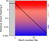 |
Fig. 1 Relative shock heating, k (Eq. (31)), as a function of Mach number, Ma, for a constant Γ1 = 1.44. For Ma < 1 there is no accretion shock, we therefore artificially set k(Ma < 1) = k(Ma = 1) = 5.16. For Ma > 1 we identify three regions: k ~ 0 corresponds to the cold-start scenario, k = 1 represents a classical hot-start scenario, and intermediate values represent a warm-start scenario. The transition around k ≈ 0.1 is chosen arbitrarily. |
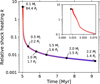 |
Fig. 2 Evolution of the relative shock heating, k, as a function of time during gas accretion of the forming giant planet in the detached phase. The data correspond to the default-case planet from Sect. 3.1. The mass and radius evolution are indicated at selected data points. The inset highlights the brief hot phase following detachment. |
3 Imprint of formation mechanisms on planetary HR diagrams
In this section, we outline our simulation setup and present the resulting planetary HR diagrams to study how the mechanisms of planetary formation manifest in HRDs. We begin by describing the default setup (Sect. 3.1) and then present an in-depth study of a single formation simulation leading to a ~2 MJ planet as our default case (Table 2 and Fig. 3). We examine the main characteristics of the L–T track throughout the formation and evolution of the planet over a period of 10 Gyr (Sect. 3.2). In the subsequent sections, we explore the influence of various parameters and assumptions on the formation process and their resulting HRD, including η for purely hot and cold starts (Sect. 3.3), the influence of contraction in the detached phase (Sect. 3.4), different planetary masses (Sect. 3.5), a core accretion scenario with pebbles instead of planetesimals (Sect. 3.6), and finally the influence of orbital migration (Sect. 3.7). All simulations are followed over a period of 200 Myr.
Initial conditions and parameters for the default in situ simulation, resulting in a planet with Mtot = 2.2 MJ.
3.1 Simulation setup for the default case
In Table 1, we summarise the initial conditions and settings of our default simulation. Following previous studies on giant planet formation (Pollack et al. 1996; Lissauer et al. 2009; D’Angelo et al. 2021), and to avoid the excessive complexity introduced by additional input physics, we base our default scenario on a single embryo, planetesimal accretion, and in situ formation. We placed the embryo at t = 0 yr at a semi-major axis of a = 5.2 au, where it remains, in a gas disc with an initial total mass of 0.04 M⊙ around a solar-type star. We used an independent and simplified profile based on the ‘minimum-mass solar nebula’ (MMSN) for the disc of planetesimals:
 (32)
(32)
We neglected the impact of ice lines, which facilitates comparison later in Sect. 3.5, where we increased the initial total disc mass, Mdisk,0, to study the formation of planets with different masses. We keep the value and structure of Σρ1ί1 unchanged in most subsequent sections to ensure low and comparable core masses.
3.2 Results for the default case
Figure 3 shows the HR diagram track of the default case, where we plot the total planetary luminosity, Ltot, against the temperature at the planet surface, Ts. We show data only for Mp > 0.025 M⊕ (approximately two lunar masses) in the HRD. Data points below this value are influenced by details of the simulation initialisation, such as the assumed dynamical state of the planetesimals. We note that Ltot excludes the fraction of the shock luminosity that is radiated away; therefore, neither the temperature nor the luminosity in this diagram account for this fraction (see Sect. 3.3 for a comparison). Except during the early attached phase, where the nebular gas temperature contributes significantly, Eq. (12) then simplifies to  . The accretion-shock radiation likely emerges from only a small fraction of the surface and is characterised by a different spectral energy distribution (SED) than that of the overall planet surface. However, it is included and visible in Lbol.
Fig. 4 shows the temporal evolution of key quantities, including luminosity, temperature, mass, radius, accretion rates, and timescales. These quantities illustrate the physical processes underlying the formation and evolution track of the planet in the HRD.
A defining feature of the tracks during formation with planetesimal accretion is the presence of three distinct branches, each corresponding to the phases outlined in Sect. 2.2: the attached, detached, or evolutionary phases. Based on the direction of evolution along these three branches, we refer to these regions as the ‘ascending branch’, the ‘planetary horizontal branch’ and the ‘descending branch’.
3.2.1 The ascending branch
The formation process of the young planet begins in the bottom-right corner of the HRD (Fig. 3) with low luminosity and surface temperature. The planet is in the attached phase and remains deeply embedded in a relatively massive protoplanetary disc. It acquires almost all of its new mass through solid accretion (Fig. 4e), so that L ≈ LM,s. Combined with the relatively large total radius, the low initial luminosity naturally leads to a cold intrinsic temperature, Tint, which is only marginally higher than the early disc midplane temperature, Td. Thus, at least initially, the disc contribution dominates the planetary surface temperature in Eq. (12). In addition, the disc temperature directly influences the outer radius of the planet. For low-mass planets, Mp ≈ Mc, and Rp ≈ RB (Lissauer et al. 2009), so that
 (33)
(33)
 (34)
(34)
where we defined  in RB (Eq. (13)) as
 (35)
(35)
Consequently, the initial slope of the ascending branch remains strongly influenced by the cooling disc, and the accretion of solids onto the small core is not sufficient to significantly heat the large, rapidly growing radius of the embedded young planet.
Later in the attached phase, the outer radius transitions from RB to  (Lissauer et al. 2009). Around that time, the influence of the disc diminishes because its temperature no longer sets the radius, and for Tint > Td, Eq. (12) reduces to T ≈ Tint. By assuming a shear-dominated velocity distribution for the planetesimals at this stage, where
  , we derive a semi-analytical approximation of the luminosity-temperature relationship, yielding L ∝ T8/Σpla (see Appendix A.2). Fig. 3 shows this trend for Σpla = 1.7 g cm−2, the median value of the surface density in the final megayear before the planet detaches. The same slope is observed for planets of various masses in the late attached phase in Fig. 7.
During the final ~ 1 Myr before detachment, the gas accretion rate, Ṁgas, finally exceeds the solid accretion rate, Ṁc. Fig. 4f shows that the ascending branch is dominated by τacc ≈ τacc,s, which also dictates τcoo1. Although τacc,g is much shorter, the envelope mass remains orders of magnitude lower than the core mass, and τacc,s therefore dominates. Only later, when τacc ≈ τacc,g, can the envelope cool and contract rapidly enough for Ṁgas to exceed the maximum disc supply rate, leading to detachment.
In the late ascending branch, τcoo1 < τKH,env because solid accretion still generates most of the luminosity, so that Ltot ≈ LM,s. The classical picture in which τKH,env defines the gas accretion rate (Ikoma et al. 2001) does not apply here due to ongoing solid accretion. The envelope mass increases primarily through the growth of the (attracting) core mass and the associated expansion of the Hill radius, rather than through envelope cooling at constant core mass, which allows new gas to stream into the envelope.
 |
Fig. 3 Hertzsprung–Russell diagram (HRD) track of the default case (final mass of 2.2 MJ; see Table 1), showing surface temperature (Eqs. (12), (19) and (21), depending on the phase) and total luminosity (Eq. (6)). Key events are marked as follows: start point (•), detachment (⋆), maximum luminosity (▼), disc dispersal (■), and the age of Jupiter (+). Table 2 lists the corresponding values for time, mass, and radius. In the ascending branch, small black triangles (▲) indicate linearly spaced time indicators every Myr. The black dots (•) represent post-detachment intervals equally spaced in log(time). Grey reference lines show two trends: the predicted slope derived in Appendix A, evaluated using the median late-attached-phase surface density of Σpla = 1.7 g cm−2 (labelled with L ∝ T8), and a constant-radius track for Rp = 1 RJ, which approximates a cooling planet in the evolutionary phase before stellar irradiation becomes relevant (last downturn). |
 |
Fig. 4 Time evolution, up to 20 Myr, of selected quantities related to (a) luminosity, (b) temperature, (c) mass, (d) radius, (e) mass accretion, and (f) timescales. In each panel, a dashed (dot-dashed) line marks the moment of detachment (disc dispersal), (a) Total luminosity emerging from the planet surface Ltot (excluding the fraction of the shock luminosity that is radiated away in the accretion shock); the part of the gas accretion shock luminosity heating the planet, |


3.2.2 The planetary horizontal branch
The detachment of the planet and the onset of the planetary horizontal branch4 appear as a sharp knee in the HRD track in Fig. 3. The planetary surface is no longer connected to the background nebula, and the radius begins to contract rapidly (Bodenheimer et al. 2000). From immediately before to immediately after detachment, the solid accretion rate reaches a sharp maximum due to the expansion of the solid feeding zone, which in turn results from the rapidly increasing mass. Shortly after detachment, the solid accretion rate decreases strongly as scattering rather than accretion occurs and the planetesimal capture radius rapidly decreases (Mordasini et al. 2012; Podolak et al. 2020). This results in a self-amplifying mechanism in which more massive cores lead to hotter (higher-entropy) planets (Mordasini 2013). The contraction timescale, τcntrctn, is equal to the cooling timescale, τcoo1, from the moment when  , approximately 50 kyr after detachment. This implies that contraction is limited by the ability to radiate away energy, that is, by envelope cooling.
The associated horizontal movement during this phase is extremely fast; in only 0.1 Myr, the surface temperature of the planet increases from 100 to 600 K. This contraction defines the planetary horizontal branch of the formation track in the HR diagram, as it is the main driver of envelope heating in cold-start-like scenarios. We show in Sect. 3.4 how contraction alone can define envelope heating and cooling without mass accretion and can therefore be the main factor of the horizontal movement in the HRD.
In these early stages of the horizontal branch, solid accretion and thus LM,s decrease significantly due to the strongly decreasing planetesimal capture radius and associated scattering. At the same time, the gas accretion rate peaks and remains high for an extended period. Gas accretion is then limited by the disc and its gas reservoir.
From Fig. 1 and the detailed comparison with classical hot-and cold-start scenarios in Sect. 3.3, it becomes apparent that our default case can be classified somewhere between a classical (or ‘extreme’) cold start from Marley et al. (2007) and a warm start. The k-factor remains in the hot or warm region (k ≳ 0.25) for only ~25 000 yr, during which the free-fall distance is still relatively small (Rout is not much larger than Rp) and thus Mach numbers are low. For the remaining ~4 Myr the k-factor is small and accretion is close to, but not completely, a cold-start scenario. This result agrees with the prediction of Marleau et al. (2019b), who show that high gas accretion rates ≥10−3 M⊕yr−1 are required for hot starts. The method yields low shock heating relative to the modest gas accretion rate and the high value Γ1 ≈ 1.44 (Eq. (31) shows that k ∝ 1/(Γ1 − 1)).
After ~1 Myr in the detached phase,  peaks5, mainly due to a decreasing Ṁgas, followed shortly afterwards by a decline in Ltot. As we verified separately (not shown), a high gas accretion rate increases the contraction rate of the planet. Thus, it is not surprising that the decrease in Ltot, which is mainly driven by Lcntrctn in a cold-start scenario, occurs shortly thereafter. The planetary interior and surface continue to heat up until the electron degeneracy in the core is high enough to induce cooling (see Sect. 3.4). From that point onwards, most of the contraction energy, Eg, is used to raise the energy level of the degenerate electrons; they do not contribute to the internal energy of the ions and therefore not to the temperature.
3.2.3 The descending branch
Approximately 2 Myr after detaching, the planet has passed its maximum luminosity and surface temperature and reached the descending branch in the HRD. As the disc dissipates, the gas accretion rate decreases continuously until the point of complete disc dispersal at 9.2 Myr. Beyond this point, when contraction is the envelope’s only energy source, L = Lcntrctn and the timescales τcool and τKH finally converge.
The inflow of grains ceases simultaneously with the gas accretion (see Sect. 2.2.3). We assumed that the grains quickly rain out of the atmosphere (Podolak 2003), so that after gas accretion stops, only the molecular opacities from Freedman et al. (2014) at solor composition remain. The resulting decrease in opacity in the outer envelope results in a certain increase in L and Τ in the HRD at the very end of the detached phase (barely visible in Fig. 4, but clearer in Fig. 5 and Fig. 8, top right). We did not investigate in detail the consequences of the exact grain opacity reduction process or the emergence of clouds, but these effects should not modify the qualitative picture.
The rest of the planet’s lifetime in the HRD is spent in the evolutionary phase in the decreasing branch, where it further contracts and cools at constant mass. Although cloud micro-physics is relevant when interpreting sufficiently precise measurements (e.g. Saumon & Marley 2008; Hinkley et al. 2023; Morley et al. 2024), it does not qualitatively affect the cooling of gas giants. Contraction stagnates at ~1 RJ because electron degeneracy pressure prevents further significant compression (e.g. Zapolsky & Salpeter 1969). The resulting slope in the HRD is given by L ∝ Τ4 from Eq. (20) at a nearly constant radius. This relation holds as long as Tint ≫ Teq. After ~4 Gyr, the planet has cooled sufficiently for stellar irradiation (Teq in Eq. (21)) to become relevant. Thus, the L–T track begins to deviate from the simple Τ ∝ L1/4 slope. Instead, the track is mainly determined by the luminosity evolution of the star (e.g. Guillot 2010).
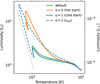 |
Fig. 5 Planetary horizontal branch up to the begin of the pure cooling (evolution) phase for the default, variable-η (green; as in Fig. 3), cold-start (blue), and hot-start (orange) start scenarios. The dashed blue line shows the unobscured bolometric luminosity, Lb0l, for a cold-start-accretion scenario (Lbol = Lint + Lacc,max; Eq. (9) with k = 0), as seen by the observer, neglecting extinction. |
3.3 Comparison with classical cold- and hot-start scenarios
Classical cold-start models (Marley et al. 2007) are not compatible with most direct-imaging observations, such as young planets in the β Pic moving group (Gratton et al. 2024). We therefore compared our default intermediate scenario with fully hot- and cold-start scenarios. To explore those cases, we replaced the factor (k − 1) in Eq. (6) with a fixed value of η = 1 (cold start) or η = 0 (hot start), so that
 (36)
(36)
Fig. 5 shows only the resulting planetary horizontal branches in the HR diagram, since the ascending branch remains unaffected by the choice of η, which only becomes relevant during the detached phase when accreted gas impacts the accretion shock at the planetary surface.
In the horizontal branch, the hot-start scenario produces hotter and more luminous planet surfaces, reaching a maximum luminosity of 1.49 × 10⁻⁴ L⊙, compared to 2.35 × 10⁻⁵ L⊙ in the default case and 2.10 × 10⁻⁵ L⊙ in the cold case. However, distinguishing between cold and hot starts based solely on bolometric luminosity would be challenging, because an observer would still see both the intrinsic and radiated shock luminosity simultaneously. Separating the shock contribution (for example, as Hα or a UV continuum; Aoyama et al. 2020; Zhou et al. 2021) from the normal photospheric emission allows one to disentangle the contributions. Interestingly, in the cold-start scenario, this sum even surpasses the luminosity of the hot-start case, despite identical gas accretion rates, reaching a maximum luminosity of 2.09 × 10⁻⁴ L⊙ This occurs because the inflated radius of the hot planet results in a lower Lacc,max, with the energy difference being radiated away later as Lcntrctn. Ultimately, the total integrated radiated energy is the same for both scenarios at the end of the simulation, except for differences caused by planetesimal accretion in the detached phase due to variations in planetary radius.
Our findings on the k-factor in Fig. 2 are linked to the early detached phase, where the approach with  (Eq. (31)) can briefly produce more luminous planets because k exceeds unity. However, as accretion progresses, Fig. 5 shows that our default approach more closely resembles a cold-start scenario than a hot-start scenario. At 4.2 Myr after detachment, the planet in our default scenario has completed its formation and its post-formation luminosity is 1.49 × 10⁻⁵ L⊙. This value lies between the cold-start (7 × 10⁻⁶ L⊙) and hot-start (1.6 × 10⁻⁵ L⊙) luminosities reported by Marley et al. (2007, their Fig. 3) for a planet of comparable mass after 4.2 Myr. The difference arises from the fact that we have a ~40% more massive core and because our accretion is not fully cold.
During most of the gas accretion phase, the luminosity of the hot-start planet in Eq. (31) is primarily governed by Lacc,max, with Lcntrctn becoming significant only once accretion ceases. In the evolutionary stage, the hot-start planet retains a radius approximately 25% larger than in the cold-start case despite similar masses, resulting in a higher luminosity due to faster contraction. The luminosity difference between the cases diminishes over time: by 1.3 Myr after formation, the hot planet is only 50% more luminous than in the default case, declining to 10% by 11.5 Myr after formation.
3.4 Evolution of contracting, non-accreting planets
Hayashi (1961) provides a pioneering study of the development of pre-main-sequence (PMS) stars in the HRD, which are now referred to as ‘Hayashi tracks’. Following rapid contraction and accretion during the protostar phase, a PMS or Τ Tauri star undergoes a slow contraction phase along the Hayashi tracks until nuclear fusion ignites, marking the star’s arrival of the main sequence (MS). For fully convective PMS stars (M⋆ ≲ 0.5 M⊙), the (downward) Hayashi tracks are almost vertical lines in the HRD. In contrast, the tracks of more massive stars (M⋆ ≳ 0.5 M⊙) curve into vertical Henyey lines due to the emergence of inner radiative zones (Henyey et al. 1955).
The formation process of giant gas planets resembles that of young proto- and PMS-stars, particularly during the detached phase. Immediately after detachment, the planet undergoes rapid contraction from an initial radius Rp = RB ~ 100 RJ to a final radius Rp ~ 2 RJ over a short period. This phase is also when gas accretion, Ṁgas, is at its peak, allowing the planet to acquire a considerable amount of its mass. This post-detachment period is akin to the protostellar scenario in which, despite rapid collapse, the object continues to accrete substantial mass from its surroundings.
Although contraction in the protostellar and planetary cases may appear similar at first glance, there are two significant distinctions. First, a planet has a significantly lower mass than a protostar, and therefore once accretion has stopped, it will never enter a burning phase if its mass is below the deuterium-burning limit. Second, the presence of a (rocky) core in planets leads to cooling effects and HR tracks that differ from classical vertical Hayashi tracks of idealised core-less stars.
The results presented in the appendices of Mollière & Mordasini (2012) show the effect of a core and electron degeneracy on envelope cooling. We tested the applicability of these effects by measuring the mass-averaged compressibility factor  , and the electron degeneracy,
  . The compressibility factor, Z, is defined for each layer i in the envelope by
 (37)
(37)
where μ is the local mean molecular mass. The mass average,
 (38)
(38)
measures how closely the envelope resembles an ideal6 gas, for which Z = 1 by definition. For Θe we followed the implementation of Mollière & Mordasini (2012) and Dewitt et al. (1973). Analogously to Eq. (38), we calculated the mass average for Θe, providing a measure of electron degeneracy for our envelope ranging from  (non-degenerate) to 0 (fully degenerate).
We explore  and
and  in Fig. 6, where we artificially turned off gas and solid accretion shortly after entering the detached phase to investigate the effect of contraction alone. The early cut-off point for gas accretion leads to an unrealistically high Mc/Menv ratio for a giant planet of ~0.8. Nonetheless, this setup allows us to study the pure contraction of a constant-mass envelope containing a core. According to Mollière & Mordasini (2012, their Appendices A and B), the planet’s interior envelope is expected to heat up initially until either a sufficiently small Rp/Rc ratio is attained or a notably high degeneracy
  is achieved. We expect heat from contraction to be generated in deep layers (Kippenhahn et al. 2013) but to be transported outward quickly by convection.
The test planet in Fig. 6 detaches with a mass of Mtot = 39.55 M⊕, Menv = 21.90 M⊕, and an initial radius of 83.11 RJ. The envelope central temperature, Ts, core, initially increases as the planet contracts to a radius of 6.37 RJ. The surface temperature continues to increase until the planetary radius has decreased to 2.52 RJ. The lower panel of Fig. 6 shows that by the time of maximum Ts,core, the envelope is already significantly degenerate ( ). We interpret this degeneracy as the main reason for the onset of the decrease in central temperature. This decrease agrees with Mollière & Mordasini (2012, their Appendix B) and is further supported by degenerate matter evolution in white dwarfs (Kippenhahn et al. 2013). This behaviour differs from the often-invoked virial theorem for ideal (non-degenerate) gases, which assumes
 (39)
(39)
Here, a decrease in gravitational energy, Ėg < 0, suggests a rise in total internal energy, Ėi resulting in a temperature increase for an ideal gas model. This heating is observed in the early stages of the forced evolution phase, where the envelope still resembles an ideal gas and electron degeneracy is low.
Because of this change in regime, the L–T track for this contracting planet clearly deviates from a perfectly vertical Hayashi track. Guillot et al. (1996) obtained a similar result when investigating the detection of 51 Peg b, as did Baraffe et al. (2002) for the evolution of low-mass substellar objects (1–20 MJ). Baraffe et al. (2002) found that objects starting their evolution with a large radius initially increase their Teff during the first megayears before cooling at later times. Our non-ideal-gas case closely resembles the theoretical scenario presented by Guillot et al. (1996) (see also the updated version in Guillot et al. 2023), in which the contracting planet avoids the forbidden superadiabatic region.
For the default-case planet, which receives an additional energy input from gas accretion beyond gravitational contraction, the maximum surface temperature is reached at  . Subsequently, the central envelope temperature reaches its maximum at
  and a radius of Rp = 1.44 RJ. Guillot (2005) estimated the present-day degeneracy parameter of Jupiter to lie in the range 0.03 < θe < 0.1, where θe = T/TF and TF denotes the electron Fermi temperature. Our simulations are consistent with this estimate, yielding θe = 0.059 (or
  ) for the default-case planet after 4.6 Gyr.
 |
Fig. 6 Top panel: planetary L–T track with a forced cessation of accretion immediately after detachment, with Mtot = 39.55 M⊕, Menv = 21.90 M⊕, and a radius of 83.11 RJ. The point of detachment and end of accretion is marked with a star. The point with maximal Ts,core = 23 500 K in the forced evolution stage is marked with a triangle, while the point with Ts,max = 436 K is marked with a dot. Bottom panel: evolution of |


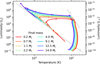 |
Fig. 7 Planetary HRD tracks for a range of final masses. We obtained the different masses by varying the initial disc gas mass at a fixed solid surface density, Σpla,5.2au = 10 g cm−2. The initial disc masses of 0.025, 0.03, 0.035, 0.04, 0.05, 0.075 and 0.1 M⊙ lead to the final masses colour-coded in the figure, in the same increasing order. Stars indicate the moment of detachment, while dashed lines connect isochrones at 104, 105, 106, and 107 yr after detachment. The most massive planet exceeds the deuterium-burning limit, resulting in an additional spike in the L–T track at the upper-left end. Otherwise, all masses share a similar overall shape of the HRD track, with three distinct branches. The 2.2 MJ planet corresponds to the default case of Sect. 3.1. The tracks are shown up to an age of 200 Myr; subsequent evolution proceeds approximately along the 1-RJ line. |
3.5 Different final masses
In Fig. 7, we present L–T tracks corresponding to planets with final total masses of Mp = 0.2–15 MJ. The difference in mass arises from adjustments in the initial total disc mass, Mdisk,0 (0.025 M⊙ to 0.1 M⊙), while keeping the properties of the solids disc fixed to those of the default case (Sect. 3.1). This approach yields comparable core masses (19–26 Μ⊕) across a wide range of total final masses. The values are not strictly identical for the following reasons. The presence of more gas in the disc leads to a stronger damping of the planetesimal inclination i and eccentricity e by the gas disc, thereby increasing the solid accretion rate. This in turn leads to a higher core mass and, eventually, a higher gas accretion rate. Moreover, a more massive disc has a higher midplane temperature (Nakamoto & Nakagawa 1994), which, as discussed in Sect. 3.1, is the main contributor to the planet’s surface temperature during the early stages of the attached phase. As a consequence, lower-mass planets exhibit cooler ascending branches and transition earlier to the horizontal branch at lower luminosities in the HRD. The resulting shock conditions lead to relatively high shock efficiencies in all simulations. The difference in luminosity can therefore be attributed to the higher gas accretion rates for more massive discs. On the one hand, a higher Ṁgas directly increases  for similar values for k. On the other hand, a higher mass accreted in the early stages leads to a higher Lcntrctn at later times because more mass is contracting.
In general, the three branches of the L–T tracks of all planets share a similar general shape. Except for the descending branch, the tracks run parallel, with more massive planets being hotter and more luminous as their accretion rates are higher. More massive planets also enter the horizontal branch at higher luminosities and temperatures because the disc-limited gas accretion rate increases with disc mass.
An exception to the similar general shape is the most massive planet, which exhibits a distinct spike in the upper-left corner of its HRD track in Fig. 7. When the spike begins, the planet has accumulated a total mass of 13.33 MJ, exceeding the deuterium-burning threshold in the absence (Saumon et al. 1996) or presence of a solid core (Spiegel et al. 2011; Mollière & Mordasini 2012; Bodenheimer et al. 2013). Consequently, the spike reflects the ignition of deuterium burning, which results in a strong increase in luminosity and a temporary radius inflation. In our variable-η scenario, which corresponds to a moderately warm start scenario,  , and deuterium burning rapidly becomes the dominant luminosity source (L ≈ LD burn).
We compared the results of Fig. 7 with those presented in Sect. 3.3. We find that the hot-start formation of a 2.2 MJ planet leads to a maximum luminosity comparable to that of a 9.2 MJ planet in a cold-start formation scenario. However, the maximum temperatures reached differ by ΔT ≈ 380 K.
While the tracks are largely parallel along the ascending and horizontal branches, they nearly overlap in the evolutionary descending branch, with the exception of the lowest-mass planet (0.2 MJ). All planets ultimately evolve with approximately the same slope once they approach the ≃1 RJ line. This degeneracy is well known (Baraffe et al. 2002) and results from the weak mass dependency of the radius and its weak evolution at later times, for sub-stellar mass bodies with M ~ 1–10 MJ (Chabrier & Baraffe 2000). By the end of our simulations at 0.2 Gyr, giant planets evolve directly from the L ∝ T4 relation. The different slope of the lowest-mass planet indicates that its less degenerate interior undergoes a more significant change in radius.
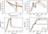 |
Fig. 8 Top-left panel: planetary HRD for a formation scenario in which the solid core grows via pebble accretion. Initial gas disc masses are 0.02 (blue), 0.03 (orange), 0.04 (green), and 0.05 M⊙ (red). The planets reach total masses of 1.4, 2.8, 4.6, and 6.7 MJ, respectively, while maintaining similar core masses of 8–10 M⊕. We show data up to 200 Myr. Other panels: time evolution of the luminosity (excluding accretion-shock luminosity), radius, and core and envelope masses. In all panels, the transition from the attached to the detached phase is marked with a dot and the time of disc dispersal by a square. |
3.6 Core-accretion scenario with pebbles
While the previous sections focussed on planet formation simulations based on the accretion of planetesimals (10 km in size; Table 1), which yield qualitatively similar L–T tracks, alternative accretion mechanisms can produce distinctly different formation histories. These differences arise from variations in the growth timescale and in the relative timing of solid and gas accretion, and consequently affect the thermal evolution of forming planets as traced in the HR diagram. One such scenario is pebble accretion (Ormel & Klahr 2010; Lambrechts & Johansen 2012; Ormel 2017), in which typically centimetre-sized particles are the primary solid building blocks. This mechanism can facilitate rapid core growth at large distances.
We present L–T tracks for simulations in which solid accretion occurs only via pebbles, using the two-population solid-disc mode of Birnstiel et al. (2012). The general implementation of this model within the Bern Model is described by Voelkel et al. (2020) and Emsenhuber et al. (2023). We used a slightly modified prescription of Ormel (2017) for the accretion of pebbles, with a sharp cut-off at the pebble isolation mass (Bitsch et al. 2018). To create planets with masses comparable to those in previous sections, we used total disc masses of Mdisk,0 = 0.02, 0.03, 0.04, 0.05 Μ⊙ and an external photoevaporation rate of Ṁwind = 10−5 M⊙yr−1.
Fig. 8 shows the L–T tracks of the four resulting planets, along with the time evolution of their luminosity (excluding accretion-shock luminosity), radius, and mass. Unsurprisingly, the most notable difference occurs during the attached phase, where the ascending branch splits into two distinct parts. During the early stages, the solid accretion timescale, τacc,s, is approximately two orders of magnitude shorter than in the planetesimal-accretion scenario, resulting in substantially higher total luminosities. During this phase, the planets rapidly ascend the initial, steep (approximately vertical) branch until pebble accretion ceases upon reaching the pebble isolation mass of about 9 Μ⊕, after roughly 60–100 kyr, depending on the initial disc mass. The pebble isolation mass is not identical because the scale height, which sets the pebble isolation mass, depends to some extent on the disc mass.
Once the pebble isolation mass is reached, the planetary luminosity is at a local maximum. For lower-mass planets, this maximum is also the global maximum. Because of this hot and luminous state, gas accretion remains low and insufficient for the planet to detach from the nebula. Kessler & Alibert (2023) present a detailed study of the suppression of gas accretion due to the high solid accretion rate with pebbles.
Following the abrupt termination of the pebble flux, the core luminosity, and hence Ltot, decreases rapidly. This subsequent cooling phase lasts approximately 0.1 Myr. During this time, the mass remains approximately constant and is still nearly equal to the core mass. The total radius Rout is already dominated by the Hill-radius term (RH/4 ≪ RB). Since Rout, scales with the Hill sphere, it also remains constant. Consequently, the tracks move diagonally downward to lower temperatures and luminosities, following L ∝ Τ4. During this phase, the temperature decreases from 200–300 Κ to about 70–80 K, which is only slightly above the disc background temperature. The tracks are therefore approximately parallel to the grey line in the top-left panel, which represents the slope of the tracks in the evolutionary (descending) branch, where the radius also varies little; however, in the present phase the radius is much larger.
This diagonal downward movement ends once gas accretion regulated by the classical KH cooling of the gaseous envelope at zero solid accretion (Ikoma et al. 2000) becomes significant. Because of gas accretion the luminosity begins to rise again. The KH-regulated gas accretion rate increases as runaway gas accretion begins and soon exceeds the disc-limited value, leading to detachment. This occurs at about 20–30 Μ⊕ and approximately 0.1 Myr after the luminosity minimum.
Thus, different solid accretion models produce clearly different tracks at early times. We note in passing that the HR tracks would likely exhibit a similar shape for hypothetical runaway planetesimal accretion (instead of oligarchic) as assumed in Pollack et al. (1996), although we have not performed such simulations directly.
Remarkably, the early luminosity peak caused by pebble accretion may reach values comparable to, or in some cases even exceeding, the maximum luminosity attained during the detached phase (rapid gas accretion), placing it, in terms of scale, in the same order of magnitude as the inferred luminosity of directly imaged forming planets such as PDS70 b (Stolker et al. 2020; Wang et al. 2021; Blakely et al. 2025). However, at this stage the planet is still deeply embedded in the protoplanetary disc, and absorption by the surrounding material likely significantly hinders its detectability. Additionally, this is a very short phase that lasts only about 10 kyr.
After the initial ascending branch phase and detachment from the disc, the subsequent planetary horizontal branch and the descending evolutionary branch closely resemble those obtained in the planetesimal accretion scenario.
 |
Fig. 9 Evolution of the semi-major axis, luminosity, radius, and total mass for three migrating planets with different initial starting location of 10 au (blue), 12 au (orange), and 14 au (green). The point of detachment is marked by a solid dot and the point of disc dispersal by a solid square. Data is shown for the formation phases and until 200 Myr of the evolution phase, rather than for the full duration as previously shown in Fig. 10. |
3.7 Migrating planets
In the previous sections, we neglected orbital migration to simplify the processes governing the formation and thermal evolution of young planets. Here, we include migration and examine its impact on the resulting L–T tracks. To this end, we considered single-embryo formation simulations with initial semi-major axes of 10, 12, and 14 au, which produce planets with total masses between 5 and 6 MJ. We also adopted the gas accretion prescription of Bodenheimer et al. (2013) and, to ensure the formation of giant planets at larger distances, we reduced the planetesimal size to 1 km. Finally, we replaced the constant power law solids disc profile (Eq. (32)) used so far with a profile that follows the gas disc, scaling the gas surface density by a constant dust-to-gas ratio fd/g = 0.03.
Fig. 10 presents the resulting HRDs of the migrating planets, together with the evolution of their mass and radius as a function of the semi-major axis. The three panels use the same markers (a)-(h) to indicate key phases and events, as annotated in the figure. To enable comparison of the respective timescales, Fig. 9 shows the evolution of a, L, Rp, and Mp over the first 200 Myr.
A short episode of enhanced planetesimal accretion during the first 10 000 yr, occurring just before the planet reaches a mass of 0.025 Μ⊕ (approximately two lunar masses) at (a), produces the prominent feature on the early ascending branch of the HRD. This behaviour is not specific to these migration runs; in the in situ simulations shown earlier, the same phase occurs at lower masses that are not shown due to the different disc setup and initialisation. The ascending branch around (b) is similar to that in the in situ case. The luminosity is dominated by solid accretion (L = LM,s), while the surface temperature remains influenced by the disc midplane temperature.
As the planet grows, the slope of the L–T track increasingly deviates from the steep ascending branches found in the in situ runs. This deviation arises from planetary migration within the disc, which modifies both the local disc conditions and the solid accretion rate. Young, low-mass planets embedded in protoplanetary discs initially undergo inward Type I migration (dashed line) (Goldreich & Tremaine 1979; Ward 1997; Papaloizou et al. 2007). Type I migration can occur at remarkably high rates, as shown in Fig. 9. For example, the planet initially located at 14 au migrates inward from 10 au to 1 au within ~0.5 Myr. As the planets sweep through the disc, there is a sudden reduction in Σpla, and thus in Ṁs, at the ice line, which produces a break in the luminosity (marker (c) in the HRD in Fig. 10). The accretion rate quickly rebounds as the planets continue migrating towards the inner disc, where planetesimal surface densities are once again higher.
Another consequence of migration is the reduction of the planetary radius during the attached phase, driven by the linear dependence of the Hill radius RH on the semi-major axis, despite the concurrent increase in planetary mass, which enters only weakly, scaling as  . Compared to the previous in situ simulations studied above, the simulations incorporating migration yield higher core masses of ~40 Μ⊕ (Ward 1989; Alibert et al. 2004, resulting in larger luminosities at the end of the ascending branch. In combination with the reduced planetary radii, this leads to higher radiative fluxes and hence to significantly higher intrinsic and surface temperatures (see Eq. (10)). In addition, inward migration places the planet in progressively hotter regions of the protoplanetary disc, further increasing the surface temperature. As a result, during the early attached phase, migrating planets follow ascending branches in the HR diagram that are shifted toward higher temperatures and inclined to the left compared to the in situ case. The resulting evolutionary tracks therefore also deviate from the previously observed L ∝ T8 relation, as migration is most rapid precisely when the approximation R ≈ RH becomes valid.
Around (e), three key transitions occur in close succession: the planet’s envelope mass becomes comparable to the core mass, Menv ≃ Mc, the planet detaches from the disc (end of the attached phase), and migration slows from Type I to Type II as the planet begins to open a gap (Papaloizou & Terquem 2006; Section 5.1 of Emsenhuber et al. 2021 and references therein). In the present simulations, we find that detachment occurs approximately when the core and envelope have the same mass (the ‘crossover point’; e.g. Pollack et al. 1996; Hubickyj et al. 2005), and that the transition from Type I to Type II precedes this by only 30–40 kyr. This near-coincidence is expected because all three events are primarily controlled by the rapid increase in planet mass: once the planet is massive enough to significantly perturb the disc (reducing the migration torque and initiating gap opening), it is also close to the onset of runaway gas accretion, causing Menv to rise rapidly and leading to detachment.
The subsequent formation and evolution of the horizontal branch, from (f) to (h), resemble the in situ simulations shown earlier. At (f), the envelopes, initially still similar to an ideal gas, contract rapidly and heat up until the overall degeneracy becomes high enough to halt the rapid contraction. From this point on at (g), while still accreting gas, the planets contract and cool. By this stage, migration has brought the planets close to the star, where irradiation slows their cooling. At the age of the Solar System, their surface temperatures are ≳500 K.
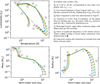 |
Fig. 10 Top panel: L–T tracks of three migrating planets with initial semi-major axes of 10 au (blue), 12 au (orange), and 14 au (green), showing their formation and evolution up to 200 Myr. Filled dots and squares indicate the points of detachment and disc dispersal, respectively. Labels (a)-(h) mark various phases of the process, as explained in the top right. Type I (Type II) migration is indicated by dashed (solid) segments. Bottom panels: mass and radius as functions of orbital distance while the planets migrate inwards. Final masses are 5–6 MJ. |
4 Discussion and conclusions
Our results illustrate the strong imprints of the main phases of the core-accretion paradigm – whether core growth proceeds through planetesimals or pebbles – on the luminosity and temperature evolution, and thus on the HRD tracks of forming planets. This impact is particularly significant during the early stages of the ascending branch. In the pebble-accretion scenario, the rapid accretion of solids leads to a brief but intense luminosity spike, with peak luminosities reaching up to ~105 LJ (~10−4 L⊙) at ages ≲0.1 Myr, during which the L–T tracks show a sharp upward trend at a nearly constant temperature. In contrast, planetesimal accretion produces a more gradual ascent at lower temperatures, reflecting the longer solid accretion timescale. This clear separation of formation pathways in the HR diagram highlights the diagnostic power of this representation, as differences in the underlying accretion physics translate directly into distinct tracks.
The high luminosities reached during the early pebble accretion phase raise interesting questions about the observability of such young, luminous, yet still embedded planets. For instance, Brunngräber & Wolf (2018), predict detections via brightness asymmetries for luminosities above L ≳ 5 × 10⁶ LJ (their test companion ℰ), measurable with the MATISSE beam combiner (Lopez et al. 2014). While the luminosities obtained in our simulations (Sect. 3.6) remain below this threshold, higher pebble isolation masses, as suggested by Bitsch et al. (2018), could potentially yield more luminous objects. A population-synthesis study would be required to explore this regime in a statistically meaningful way. In this embedded early phase, luminosity may be the main observational tracer of young, low-mass planets, as they are not expected to open gaps or generate detectable disc substructures in Class 0/I systems (Nazari et al. 2025). High luminosity could also help make even low-mass planets detectable with the Atacama Large Millimeter/submillimeter Array (ALMA) through their indirect effects on disc chemistry (e.g. Yoshida et al. 2026).
More generally, planetary HRDs provide insight into the importance of the physical processes governing the luminosity and surface temperature of a planet at different formation stages. Heating and cooling due to contraction, gas accretion, and orbital migration imprint distinct signatures on the tracks, allowing the dominant energy source to be identified from the location and slope in the HRD. In contrast to time-based evolutionary representations, the HRD makes these different contributions apparent through changes in track shape.
Identifying the dominant luminosity sources during formation is also a prerequisite for constructing realistic SEDs of young, forming planets and for interpreting accretion-related observables. Our treatment of the accretion shock provides a starting point for a more detailed analysis of emission diagnostics such as Hα during the formation phase. However, the present model does not account for more complex gas accretion geometries through a circumplanetary disc (e.g. Ward & Canup 2010; Zhu 2015; Szulágyi et al. 2019), which we will investigate in future work. A natural next step is to couple the thermal-evolution tracks to circumplanetary disc accretion and radiative-transfer calculations in order to predict full SEDs, as well as observable magnitudes and colours, rather than intrinsic bolometric luminosities alone. This will enable direct comparisons in formats such as colour-magnitude diagrams and will help assess how accretion geometry and reprocessing in the CPD modify the inferred effective temperatures and luminosities (e.g. Aoyama et al. 2020; Marleau et al. 2022; Adams & Batygin 2022; Marleau et al. 2023; Choksi & Chiang 2025; Taylor et al. 2026). In this context, explaining the high entropies (hot starts) inferred for some directly imaged planets (e.g. Gratton et al. 2024) remains an open challenge unless relatively massive cores provide the necessary heating (Mordasini 2013).
In this comparison it is important to distinguish between ‘bare’ young planets with weak or negligible ongoing accretion and a faint (or absent) circumplanetary disc, and very young, still embedded, actively accreting planets. The L–T tracks presented in this work describe the evolution of the planet as driven primarily by its interior. These tracks are therefore most directly comparable to the former category, for which the observed emission is expected to be dominated by the planet photosphere.
However, for more embedded, strongly accreting objects, the emergent spectrum and broadband magnitudes can be dominated by contributions from the accretion shock and the circumplanetary disc itself, as well as by reprocessing of the planetary emission, making a direct comparison to intrinsic L–T tracks less meaningful. Extending the planetary HRD concept into this regime requires forward modelling that consistently combines photospheric emission, accretion-shock luminosity, and circum-planetary disc emission into synthetic SEDs and colours, providing a pathway towards interpreting young planets in colour-magnitude space and towards a more complete observational classification across formation stages. Steps in this direction have recently appeared in the literature (Sun et al. 2024, 2026).
With this limitation in mind, we compared the tracks with observed and synthetic planets. In Fig. 11, we show selected data from the NASA Exoplanet Archive for directly imaged companions along with population synthesis data from Emsenhuber et al. (2021) and L–T tracks of migrating planets from this work. The position of the directly imaged companions in the HRD provides a qualitative indication of their formation phase or evolutionary stage. Apart from PDS70 b/c and WISPIT 2 b (discussed in the following), all objects lie close to the l RJ line characterising the descending evolutionary branch. This is expected, since the listed companions are mostly found in systems without significant accretion discs, indicating that accretion has already terminated or is nearly complete.
Data points from the population synthesis of Emsenhuber et al. (2021) accumulate in the upper-left region. A key reason for this is that the population we used, ‘NG76’, assumes the classical hot-start scenario (η = 0), leading to hot and luminous planets even below the brown-dwarf threshold. In addition, the broad mass range of the sample (~1–30 MJ) further contributes to this pattern; the most luminous objects in the upper-left corner predominantly correspond to higher-mass planets and brown dwarfs (16 of the total 82 planets shown end up with a mass above the deuterium-burning limit), while lower-mass objects occupy the fainter, cooler part of the distribution. PDS70 b/c might eventually reach the upper-left region, since a cold-start scenario appears to be ruled out for these planets (Trevascus et al. 2025). Alternatively, as may also be the case for WISPIT 2 b, if their formation is already complete and they have entered the pure cooling phase, they may start from slightly larger radii than other objects.
Our L–T tracks show only the planet’s total intrinsic luminosity and not the luminosity that would be observed. Depending on the fate of the shock luminosity, for example through absorption, the observable quantity would instead be Lbol, which also includes the luminosity emitted at the accretion shock. Sect. 3.3 illustrates that the observed luminosity can be up to an order of magnitude higher than the intrinsic luminosity in cold-start scenarios (Fig. 5). Thus, the position of PDS70 b in the HRD is to some extent also compatible with the tracks of lower-mass planets with ~1 MJ.
Altogether, the tracks presented here provide a framework for interpreting the luminosity–temperature evolution of forming and young giant planets in a representation analogous to the stellar HRD, a concept well established in astronomy. Placing directly imaged companions in the planetary HRD, together with model tracks, can help identify whether an object is plausibly still accreting, undergoing rapid post-detachment contraction, or already evolving on a near-constant-mass cooling track. At present, however, because of the difficulty of detecting deeply embedded planets, the directly imaged sample is small and biased toward relatively evolved, weakly accreting (or non-accreting) objects, so that the use of planetary HRDs for population-level inferences remains largely prospective. In this sense, the planetary HRD offers a physically motivated way to relate observed luminosities and inferred temperatures to formation histories, while keeping in mind that additional processes affecting observability (extinction and absorption) must be treated separately.
The work presented here extends the well-known HRD framework to the context of planet formation. This provides an intuitive way to link observed luminosities and temperatures to formation physics and also lays the groundwork for future studies that aim to classify directly imaged young planets. However, it will be challenging to observationally populate the short early phases of the planetary horizontal branch. As discussed in Sect. 3.2.2 and seen in the population-synthesis snapshots in Fig. 11, because the horizontal branch phase is brief, only a small fraction of objects are expected to be caught there in any given snapshot, making it intrinsically difficult to build a large observed sample in that region. In practice, detecting even earlier stages on the ascending branch will be further complicated by absorption and reprocessing within the disc and envelope surrounding the forming planet.
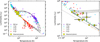 |
Fig. 11 Left panel: L–T tracks for migrating planets from Fig. 10 (grey lines), overlaid with directly imaged companions from Table 3 (yellow squares). We show planets from the NG76 hot-start population (η = 0) synthesis (Emsenhuber et al. 2021), taken from the Data Analysis Centre for Exoplanets (DACE)7, at five different times (coloured dots). We display only planets with a final mass Mp ≥ 0.9MJ. Of the 82 synthetic planets, 16 exceed the deuterium-burning limit. Right panel: zoom-in on the young directly imaged planets. Numbering follows Table 3. |
5 Summary
This study explored the concept of a ‘planetary Hertzsprung–Russell diagram (HRD)’, extending the traditional stellar HRD to planetary systems and explicitly including the formation phase of gas giants. Similar to the stellar case, the planetary HRD displays the surface temperature Ts against the total luminosity emerging from the surface, Ltot. The planetary HRD provides a framework for visualising and analysing planetary formation tracks across diverse scenarios. In this work, we used tracks computed self-consistently with a detailed 1D global giant planet formation model based on the core accretion paradigm, the Generation III Bern model (Emsenhuber et al. 2021).
We emphasise that this first paper is a theoretical study. Given the known simplifications and limitations of the model used here, which are particularly relevant for comparisons with observations – such as the absence of a CPD or the treatment of absorption and extinction – our main goal is not yet to make direct observational predictions. Instead, we aim to provide a theoretical context for the processes governing planet formation and their expression in a hitherto little-explored way, thereby establishing the basis for future links between formation theory and current, as well as future, observations of directly imaged planets, forming planets, and protoplanetary discs. Expanding on these aspects will be the subject of future work.
The main results can be summarised as follows:
In the scenario in which the solid core forms via plan-etesimal accretion (Sect. 3.1), the L–T tracks show three distinct branches corresponding to the main phases of giant planet formation (Bodenheimer et al. 2000; Mordasini et al. 2012): an ascending branch during the attached phase, a planetary horizontal branch shaped by rapid radius contraction and runaway gas accretion during the detached phase, and a descending branch during post-formation evolution (cooling) at constant mass (Fig. 3);
In the ascending branch (Sect. 3.2.1), where planets move approximately vertically upward in the HR diagram, the luminosity is primarily set by the accretion of solids (L ≈ LM,s), while Ts remains significantly influenced by the temperature of the background nebula via
 . Typically, Ts is low due to the extended planetary radius in the attached phase (Rp ~ 100 RJ). In the late attached phase, when Rp ≈ RH/4 and Tint ≫ Td, we analytically derive the scaling L ∝ T8 for in situ planetesimal accretion (Appendix A). This explains the slope in the numerical simulations;
The planetary horizontal branch (Sect. 3.2.2), where planets move approximately horizontally to the left, begins with the onset of disc-limited gas accretion and detachment from the disc. Detachment typically occurs shortly (a few 10 kyr) after crossover (Mc = Menv) is reached and rapid gas accretion begins. Detachment appears as a sharp knee in the L–T track. The subsequent rapid contraction from very large radii down to a few Jovian radii leads to a nearly horizontal motion: a strong increase in Ts from Td ~ 100 K to ~1000–1500 K, accompanied by a modest increase in Ltot. This occurs over short timescales (~105 yr);
The descending branch (Sect. 3.2.3) begins once electron degeneracy becomes important. At this point, the radius becomes only weakly dependent on temperature, which in turn halts rapid contraction. This produces another knee in the L–T track. Further evolution occurs at nearly constant radius, which decreases from ≈2 to 1 RJ over gigayear timescales. The L–T tracks follow L ~ T4; planets move diagonally downward to the right in the HRD. This holds until stellar irradiation becomes relevant for the temperature at late times;
For the first time, we replace the usual assumption of fixed hot or cold accretion (via a constant heating efficiency) by a time-dependent relative shock heating factor k (Sect. 2.2.4) based on radiation-hydrodynamic simulations (Marleau et al. 2017, 2019b, 2023). We find that spherically symmetric gas accretion yields a brief warm-to-hot accretion period shortly after detachment, but that k later becomes small, corresponding to cold accretion for most of the runaway gas accretion phase;
We studied L–T tracks for final planet masses ranging between 0.2 and 15 MJ (Sect. 3.5). The basic shape of ascending, horizontal, and descending branches is retained in all cases. The formation of higher-mass planets leads to more luminous and hotter tracks in the HRD compared to those of lower-mass counterparts. For sufficiently massive objects (Mp ≳ 13 MJ), deuterium burning generates a distinctive spike in the track towards the upper-left knee, near the transition from the horizontal to the descending branch (Fig. 7);
In the scenario in which core accretion proceeds via pebbles (Sect. 3.6), the attached phase splits into two stages: an early, brief, high-luminosity phase while pebble accretion is active, followed by a cooling phase at nearly constant core mass before Kelvin–Helmholtz-regulated gas accretion triggers detachment. This significantly alters the form of the L–T tracks. The initial phase, in which the luminosity is powered by solid accretion, is still present as a steep ascending track until the pebble isolation mass is reached. The subsequent cooling translates into an intermediate descending cooling track with L ∝ T4 (with the radius equal to RH and an initially weakly increasing envelope mass) until detachment is reached, when gas accretion attains the disclimited value. The ensuing planetary horizontal branch then appears with a slope towards higher luminosities than in the planetesimal case, because the absence of solid accretion leads to a less luminous starting point for the rapid horizontal movement. Additionally, the cooling following the first phase means that the horizontal branch crosses the early steep ascending branch;
We studied the effect of orbit migration (Sect. 3.7). Migration shifts the attached-phase tracks to higher Ts and modifies their slopes, because planets move into hotter disc regions and because R ~ RH ∝ a decreases during inward migration;
Placing observed and synthetic planets together with L–T tracks of migrating planets in the planetary HRD (Fig. 11) provides a qualitative indication of the formation phase or evolutionary stage of directly imaged companions in Table 3.
Acknowledgements
B.G. and C.M. acknowledge the support from the Swiss National Science Foundation under grant 200021_204847 “PlanetsInTime”. G.-D.M. acknowledges the support of the Deutsche Forschungsgemeinschaft (DFG) through grant MA 9185/2-1. Part of this work has been carried out within the framework of the NCCR PlanetS supported by the Swiss National Science Foundation under grants 51NF40_182901 and 51NF40_205606. Calculations were performed on the horus clusters of the Division of Space Research and Planetary Sciences at the University of Bern.
References
- Adams, F. C., & Batygin, K. 2022, ApJ, 934, 111 [Google Scholar]
- Ali-Dib, M., Cumming, A., & Lin, D. N. C. 2020, MNRAS, 494, 2440 [Google Scholar]
- Alibert, Y., Mordasini, C., & Benz, W. 2004, A&A, 417, L25 [NASA ADS] [CrossRef] [EDP Sciences] [Google Scholar]
- Aoyama, Y., Marleau, G.-D., Mordasini, C., & Ikoma, M. 2020, arXiv, [arXiv:2011.06608] [Google Scholar]
- Armitage, P. J. 2020, Astrophysics of Planet Formation, 2nd edn. (Cambridge University Press) [Google Scholar]
- Asensio-Torres, R., Henning, T., Cantalloube, F., et al. 2021, A&A, 652, A101 [NASA ADS] [CrossRef] [EDP Sciences] [Google Scholar]
- Bailey, A. P., & Zhu, Z. 2024, MNRAS, 534, 2953 [Google Scholar]
- Baraffe, I., Chabrier, G., Allard, F., & Hauschildt, P. H. 2002, A&A, 382, 563 [CrossRef] [EDP Sciences] [Google Scholar]
- Baraffe, I., Vorobyov, E., & Chabrier, G. 2012, ApJ, 756, 118 [NASA ADS] [CrossRef] [Google Scholar]
- Baraffe, I., Homeier, D., Allard, F., & Chabrier, G. 2015, A&A, 577, A42 [NASA ADS] [CrossRef] [EDP Sciences] [Google Scholar]
- Baraffe, I., Elbakyan, V. G., Vorobyov, E. I., & Chabrier, G. 2017, A&A, 597, A19 [NASA ADS] [CrossRef] [EDP Sciences] [Google Scholar]
- Bell, K. R., & Lin, D. N. C. 1994, ApJ, 427, 987 [NASA ADS] [CrossRef] [Google Scholar]
- Benisty, M., Bae, J., Facchini, S., et al. 2021, ApJ, 916, L2 [NASA ADS] [CrossRef] [Google Scholar]
- Berardo, D., & Cumming, A. 2017, ApJ, 846, L17 [NASA ADS] [CrossRef] [Google Scholar]
- Berardo, D., Cumming, A., & Marleau, G.-D. 2017, ApJ, 834, 149 [NASA ADS] [CrossRef] [Google Scholar]
- Bhandare, A., Ali Ahmad, A., & Commerçon, B. 2025, A&A, 702, L7 [NASA ADS] [CrossRef] [EDP Sciences] [Google Scholar]
- Birnstiel, T., Klahr, H., & Ercolano, B. 2012, A&A, 539, A148 [NASA ADS] [CrossRef] [EDP Sciences] [Google Scholar]
- Bitsch, B., Morbidelli, A., Johansen, A., et al. 2018, A&A, 612, A30 [NASA ADS] [CrossRef] [EDP Sciences] [Google Scholar]
- Blackman, J., Mordasini, C., Marleau, G.-D., et al. 2026, [arXiv:2606.14844] [Google Scholar]
- Blakely, D., Johnstone, D., Cugno, G., et al. 2025, AJ, 169, 137 [Google Scholar]
- Boccaletti, A., Chauvin, G., Mouillet, D., et al. 2020, arXiv e-prints [arXiv:2003.05714] [Google Scholar]
- Bodenheimer, P., D’Angelo, G., Lissauer, J. J., Fortney, J. J., & Saumon, D. 2013, ApJ, 770, 120 [NASA ADS] [CrossRef] [Google Scholar]
- Bodenheimer, P., Hubickyj, O., & Lissauer, J. J. 2000, Icarus, 143, 2 [Google Scholar]
- Bohn, A. J., Kenworthy, M. A., Ginski, C., et al. 2020, ApJ, 898, L16 [Google Scholar]
- Brunngräber, R., & Wolf, S. 2018, A&A, 611, A90 [NASA ADS] [CrossRef] [EDP Sciences] [Google Scholar]
- Burn, R., & Mordasini, C. 2024, in Handbook of Exoplanets, 143 [Google Scholar]
- Carter, A. L., Hinkley, S., Kammerer, J., et al. 2023, ApJ, 951, L20 [NASA ADS] [CrossRef] [Google Scholar]
- Cassisi, S., Potekhin, A. Y., Pietrinferni, A., Catelan, M., & Salaris, M. 2007, ApJ, 661, 1094 [NASA ADS] [CrossRef] [Google Scholar]
- Chabrier, G., & Baraffe, I. 2000, ARA&A, 38, 337 [Google Scholar]
- Chabrier, G., & Debras, F. 2021, ApJ, 917, 4 [NASA ADS] [CrossRef] [Google Scholar]
- Chen, X., & Szulágyi, J. 2022, MNRAS, 516, 506 [NASA ADS] [CrossRef] [Google Scholar]
- Choksi, N., & Chiang, E. 2025, MNRAS, 537, 2945 [Google Scholar]
- Christiaens, V., Cantalloube, F., Casassus, S., et al. 2019, ApJ, 877, L33 [Google Scholar]
- Cimerman, N. P., Kuiper, R., & Ormel, C. W. 2017, MNRAS, 471, 4662 [Google Scholar]
- Close, L. M., van Capelleveen, R. F., Weible, G., et al. 2025, ApJ, 990, L9 [Google Scholar]
- Commerçon, B., Audit, E., Chabrier, G., & Chièze, J.-P. 2011, A&A, 530, A13 [NASA ADS] [CrossRef] [EDP Sciences] [Google Scholar]
- Cumming, A., Helled, R., & Venturini, J. 2018, MNRAS, 477, 4817 [Google Scholar]
- D’Angelo, G., Weidenschilling, S. J., Lissauer, J. J., & Bodenheimer, P. 2021, Icarus, 355, 114087 [CrossRef] [Google Scholar]
- Dewitt, H. E., Graboske, H. C., & Cooper, M. S. 1973, ApJ, 181, 439 [Google Scholar]
- Drake, R. P. 2006, High-Energy-Density Physics: Fundamentals, Inertial Fusion, and Experimental Astrophysics (Berlin: Springer) [Google Scholar]
- Dupuy, T. J., Brandt, G. M., & Brandt, T. D. 2022, MNRAS, 509, 4411 [Google Scholar]
- Emsenhuber, A., Mordasini, C., Burn, R., et al. 2021, A&A, 656, A69 [NASA ADS] [CrossRef] [EDP Sciences] [Google Scholar]
- Emsenhuber, A., Burn, R., Weder, J., et al. 2023, A&A, 673, A78 [NASA ADS] [CrossRef] [EDP Sciences] [Google Scholar]
- Feldt, M., Bertram, T., Correia, C., et al. 2024, Exp. Astron., 58, 20 [Google Scholar]
- Fortney, J. J., Marley, M. S., Hubickyj, O., Bodenheimer, P., & Lissauer, J. J. 2005, Astron. Nachr., 326, 925 [NASA ADS] [CrossRef] [Google Scholar]
- Fortney, J. J., Marley, M. S., Saumon, D., & Lodders, K. 2008, ApJ, 683, 1104 [Google Scholar]
- Freedman, R. S., Marley, M. S., & Lodders, K. 2008, ApJS, 174, 504 [NASA ADS] [CrossRef] [Google Scholar]
- Freedman, R. S., Lustig-Yaeger, J., Fortney, J. J., et al. 2014, ApJS, 214, 25 [CrossRef] [Google Scholar]
- Geroux, C., Baraffe, I., Viallet, M., et al. 2016, A&A, 588, A85 [NASA ADS] [CrossRef] [EDP Sciences] [Google Scholar]
- Ghosh, P., & Lamb, F. K. 1979, ApJ, 232, 259 [Google Scholar]
- Goldreich, P., & Tremaine, S. 1979, ApJ, 233, 857 [Google Scholar]
- Gratton, R., Bonavita, M., Mesa, D., et al. 2024, A&A, 684, A69 [NASA ADS] [CrossRef] [EDP Sciences] [Google Scholar]
- Guillot, T. 2005, AREPS, 33, 493 [NASA ADS] [Google Scholar]
- Guillot, T. 2010, A&A, 520, A27 [NASA ADS] [CrossRef] [EDP Sciences] [Google Scholar]
- Guillot, T., Burrows, A., Hubbard, W. B., Lunine, J. I., & Saumon, D. 1996, ApJ, 459, L35 [Google Scholar]
- Guillot, T., Fletcher, L. N., Helled, R., et al. 2023, in Astronomical Society of the Pacific Conference Series, 534, Protostars and Planets VII, eds. S., Inutsuka, Y., Aikawa, T., Muto, K., Tomida, & M., Tamura, 947 [Google Scholar]
- Haffert, S. Y., Bohn, A. J., de Boer, J., et al. 2019, NatAs, 3, 749 [Google Scholar]
- Hartmann, L., Hewett, R., & Calvet, N. 1994, ApJ, 426, 669 [Google Scholar]
- Hashimoto, J., Aoyama, Y., Konishi, M., et al. 2020, AJ, 159, 222 [Google Scholar]
- Hayashi, C. 1961, PASJ, 13, 450 [NASA ADS] [Google Scholar]
- Helled, R., & Stevenson, D. J. 2024, AGU Adv., 5, e2024AV001171 [NASA ADS] [CrossRef] [Google Scholar]
- Henyey, L. G., Lelevier, R., & Levée, R. D. 1955, PASP, 67, 154 [NASA ADS] [CrossRef] [Google Scholar]
- Hertzsprung, E. 1909, Astron. Nachr., 179, 373 [Google Scholar]
- Hinkley, S., Lacour, S., Marleau, G.-D., et al. 2023, A&A, 671, L5 [NASA ADS] [CrossRef] [EDP Sciences] [Google Scholar]
- Hosokawa, T., & Omukai, K. 2009, ApJ, 691, 823 [Google Scholar]
- Hubickyj, O., Bodenheimer, P., & Lissauer, J. J. 2005, Icarus, 179, 415 [NASA ADS] [CrossRef] [Google Scholar]
- Ikoma, M., Nakazawa, K., & Emori, H. 2000, ApJ, 537, 1013 [NASA ADS] [CrossRef] [Google Scholar]
- Ikoma, M., Emori, H., & Nakazawa, K. 2001, ApJ, 553, 999 [NASA ADS] [CrossRef] [Google Scholar]
- Isella, A., Benisty, M., Teague, R., et al. 2019, ApJ, 879, L25 [Google Scholar]
- Keppler, M., Benisty, M., Müller, A., et al. 2018, A&A, 617, A44 [NASA ADS] [CrossRef] [EDP Sciences] [Google Scholar]
- Kessler, A., & Alibert, Y. 2023, A&A, 674, A144 [NASA ADS] [CrossRef] [EDP Sciences] [Google Scholar]
- Kippenhahn, R., Weigert, A., & Weiss, A. 2013, Stellar Structure and Evolution, Astronomy and Astrophysics Library (Berlin, Heidelberg: Springer) [Google Scholar]
- Lambrechts, M., & Johansen, A. 2012, A&A, 544, A32 [NASA ADS] [CrossRef] [EDP Sciences] [Google Scholar]
- Lissauer, J. J., Hubickyj, O., D’Angelo, G., & Bodenheimer, P. 2009, Icarus, 199, 338 [NASA ADS] [CrossRef] [Google Scholar]
- Lodato, G., Dipierro, G., Ragusa, E., et al. 2019, MNRAS, 486, 453 [Google Scholar]
- Lopez, B., Lagarde, S., Jaffe, W., et al. 2014, The Messenger, 157, 5 [NASA ADS] [Google Scholar]
- Lovis, C., Blind, N., Chazelas, B., et al. 2022, SPIE Conf. Ser., 12184, 121841Q [NASA ADS] [Google Scholar]
- Lovis, C., Blind, N., Chazelas, B., et al. 2024, arXiv e-prints [arXiv:2409.02875] [Google Scholar]
- Lynden-Bell, D., & Pringle, J. E. 1974, MNRAS, 168, 603 [Google Scholar]
- Madurowicz, A., Ruffio, J.-B., Macintosh, B., et al. 2025, AJ, 170, 326 [Google Scholar]
- Marleau, G.-D., & Cumming, A. 2014, MNRAS, 437, 1378 [Google Scholar]
- Marleau, G.-D., Klahr, H., Kuiper, R., & Mordasini, C. 2017, ApJ, 836, 221 [Google Scholar]
- Marleau, G.-D., Coleman, G. A. L., Leleu, A., & Mordasini, C. 2019a, A&A, 624, A20 [NASA ADS] [CrossRef] [EDP Sciences] [Google Scholar]
- Marleau, G.-D., Mordasini, C., & Kuiper, R. 2019b, ApJ, 881, 144 [Google Scholar]
- Marleau, G.-D., Aoyama, Y., Kuiper, R., et al. 2022, A&A, 657, A38 [NASA ADS] [CrossRef] [EDP Sciences] [Google Scholar]
- Marleau, G.-D., Kuiper, R., Béthune, W., & Mordasini, C. 2023, ApJ, 952, 89 [NASA ADS] [CrossRef] [Google Scholar]
- Marleau, G.-D., Henning, T., van Boekel, R., et al. 2025, arXiv e-prints [arXiv:2511.10751] [Google Scholar]
- Marley, M. S., Fortney, J. J., Hubickyj, O., Bodenheimer, P., & Lissauer, J. J. 2007, ApJ, 655, 541 [Google Scholar]
- Mazoyer, J., Goulas, C., Vidal, F., et al. 2024, arXiv e-prints [arXiv:2406.18424] [Google Scholar]
- Moldenhauer, T. W., Kuiper, R., Kley, W., & Ormel, C. W. 2022, A&A, 661, A142 [NASA ADS] [CrossRef] [EDP Sciences] [Google Scholar]
- Mollière, P., & Mordasini, C. 2012, A&A, 547, A105 [NASA ADS] [CrossRef] [EDP Sciences] [Google Scholar]
- Mordasini, C. 2013, A&A, 558, A113 [NASA ADS] [CrossRef] [EDP Sciences] [Google Scholar]
- Mordasini, C., Alibert, Y., Georgy, C., et al. 2012, A&A, 547, A112 [NASA ADS] [CrossRef] [EDP Sciences] [Google Scholar]
- Mordasini, C., Klahr, H., Alibert, Y., Miller, N., & Henning, T. 2014, A&A, 566, A141 [NASA ADS] [CrossRef] [EDP Sciences] [Google Scholar]
- Mordasini, C., Marleau, G.-D., & Mollière, P. 2017, A&A, 608, A72 [NASA ADS] [CrossRef] [EDP Sciences] [Google Scholar]
- Morley, C. V., Mukherjee, S., Marley, M. S., et al. 2024, ApJ, 975, 59 [NASA ADS] [CrossRef] [Google Scholar]
- Müller, A., Keppler, M., Henning, T., et al. 2018, A&A, 617, L2 [Google Scholar]
- Muzerolle, J., Calvet, N., & Hartmann, L. 1998, ApJ, 492, 743 [NASA ADS] [CrossRef] [Google Scholar]
- Nakamoto, T., & Nakagawa, Y. 1994, ApJ, 421, 640 [Google Scholar]
- Nazari, P., Sellek, A. D., & Rosotti, G. P. 2025, A&A, 697, A84 [NASA ADS] [CrossRef] [EDP Sciences] [Google Scholar]
- Nielsen, E. L., De Rosa, R. J., Macintosh, B., et al. 2019, AJ, 158, 13 [Google Scholar]
- Oberg, N., Kamp, I., Cazaux, S., Rab, C., & Czoske, O. 2023, A&A, 670, A74 [NASA ADS] [CrossRef] [EDP Sciences] [Google Scholar]
- Ormel, C. W. 2014, ApJ, 789, L18 [Google Scholar]
- Ormel, C. W. 2017, in Astrophysics and Space Science Library, 445, Formation, Evolution, and Dynamics of Young Solar Systems, eds. M. Pessah, & O., Gressel, 197 [NASA ADS] [CrossRef] [Google Scholar]
- Ormel, C. W., & Klahr, H. H. 2010, A&A, 520, A43 [NASA ADS] [CrossRef] [EDP Sciences] [Google Scholar]
- Ormel, C. W., Shi, J.-M., & Kuiper, R. 2015, MNRAS, 447, 3512 [Google Scholar]
- Papaloizou, J. C. B., & Terquem, C. 2006, Rep. Prog. Phys, 69, 119 [Google Scholar]
- Papaloizou, J. C. B., Nelson, R. P., Kley, W., Masset, F. S., & Artymowicz, P. 2007, in Protostars and Planets V, eds. B., Reipurth, D., Jewitt, & K., Keil, 655 [Google Scholar]
- Pinte, C., van der Plas, G., Ménard, F., et al. 2019, NatAs, 3, 1109 [Google Scholar]
- Pinte, C., Price, D. J., Ménard, F., et al. 2020, ApJ, 890, L9 [CrossRef] [Google Scholar]
- Podolak, M. 2003, Icarus, 165, 428 [NASA ADS] [CrossRef] [Google Scholar]
- Podolak, M., Pollack, J. B., & Reynolds, R. T. 1988, Icarus, 73, 163 [NASA ADS] [CrossRef] [Google Scholar]
- Podolak, M., Haghighipour, N., Bodenheimer, P., Helled, R., & Podolak, E. 2020, ApJ, 899, 45 [NASA ADS] [CrossRef] [Google Scholar]
- Pollack, J. B., Hubickyj, O., Bodenheimer, P., et al. 1996, Icarus, 124, 62 [NASA ADS] [CrossRef] [Google Scholar]
- Polman, J., & Mordasini, C. 2024, A&A, 692, A202 [NASA ADS] [CrossRef] [EDP Sciences] [Google Scholar]
- Prialnik, D., & Livio, M. 1985, MNRAS, 216, 37 [NASA ADS] [Google Scholar]
- Ravet, M., Bonnefoy, M., Chauvin, G., et al. 2025, A&A, 704, A325 [NASA ADS] [CrossRef] [EDP Sciences] [Google Scholar]
- Russell, H. N. 1914, Popul. Astron., 22, 275 [Google Scholar]
- Ruzza, A., Lodato, G., Rosotti, G. P., & Armitage, P. J. 2025, A&A, 700, A190 [NASA ADS] [CrossRef] [EDP Sciences] [Google Scholar]
- Safronov, V. S. 1984, in Planetary Rings, ed. A., Brahic, 647 [Google Scholar]
- Samland, M., Mollière, P., Bonnefoy, M., et al. 2017, A&A, 603, A57 [NASA ADS] [CrossRef] [EDP Sciences] [Google Scholar]
- Saumon, D., Hubbard, W. B., Burrows, A., et al. 1996, ApJ, 460, 993 [Google Scholar]
- Saumon, D., & Marley, M. S. 2008, ApJ, 689, 1327 [Google Scholar]
- Savignac, V., & Lee, E. J. 2024, ApJ, 973, 85 [NASA ADS] [CrossRef] [Google Scholar]
- Shakura, N. I., & Sunyaev, R. A. 1973, A&A, 500, 33 [NASA ADS] [Google Scholar]
- Shibaike, Y., & Mordasini, C. 2024, A&A, 687, A166 [NASA ADS] [CrossRef] [EDP Sciences] [Google Scholar]
- Spiegel, D. S., & Burrows, A. 2012, ApJ, 745, 174 [Google Scholar]
- Spiegel, D. S., Burrows, A., & Milsom, J. A. 2011, ApJ, 727, 57 [Google Scholar]
- Stolker, T., Marleau, G.-D., Cugno, G., et al. 2020, A&A, 644, A13 [NASA ADS] [CrossRef] [EDP Sciences] [Google Scholar]
- Sun, X., Huang, P., Dong, R., & Liu, S.-F. 2024, ApJ, 972, 25 [Google Scholar]
- Sun, X., Marleau, G.-D., & Liu, S.-F. 2026, A&A accepted, [arXiv:2606.08996] [Google Scholar]
- Szulágyi, J., Dullemond, C. P., Pohl, A., & Quanz, S. P. 2019, MNRAS, 487, 1248 [Google Scholar]
- Takami, M., Otten, G., Absil, O., et al. 2025, PASP, 137, 034504 [Google Scholar]
- Taylor, A. G., Adams, F. C., & Calvet, N. 2026, Icarus, 447, 116913 [Google Scholar]
- Thanathibodee, T., Calvet, N., Bae, J., Muzerolle, J., & Hernández, R. F. 2019, ApJ, 885, 94 [NASA ADS] [CrossRef] [Google Scholar]
- Trevascus, D., Blunt, S., Christiaens, V., et al. 2025, A&A, 698, A19 [NASA ADS] [CrossRef] [EDP Sciences] [Google Scholar]
- van Capelleveen, R. F., Ginski, C., Kenworthy, M. A., et al. 2025, ApJ, 990, L8 [Google Scholar]
- Vaytet, N., Chabrier, G., Audit, E., et al. 2013, A&A, 557, A90 [NASA ADS] [CrossRef] [EDP Sciences] [Google Scholar]
- Vigan A. Fontanive C. Meyer M. et al. 2021 A&A 651 A72 [NASA ADS] [CrossRef] [EDP Sciences] [Google Scholar]
- Vila, E., Amiot, P., Berné, O., et al. 2025, A&A, 704, L3 [NASA ADS] [CrossRef] [EDP Sciences] [Google Scholar]
- Voelkel, O., Klahr, H., Mordasini, C., Emsenhuber, A., & Lenz, C. 2020, A&A, 642, A75 [NASA ADS] [CrossRef] [EDP Sciences] [Google Scholar]
- Wagner, K., Follete, K. B., Close, L. M., et al. 2018, ApJ, 863, L8 [Google Scholar]
- Wang, J. J., Ginzburg, S., Ren, B., et al. 2020, AJ, 159, 263 [Google Scholar]
- Wang, J. J., Vigan, A., Lacour, S., et al. 2021, AJ, 161, 148 [Google Scholar]
- Ward, W. R. 1989, ApJ, 345, L99 [CrossRef] [Google Scholar]
- Ward, W. R. 1997, Icarus, 126, 261 [Google Scholar]
- Ward W. R. & Canup R. M. 2010 AJ 140 1168 [Google Scholar]
- Xuan, J. W., Ruffio, J.-B., Chachan, Y., et al. 2026, ApJ, 1000, 27 [Google Scholar]
- Yoshida, T. C., Alarcón, F., Bae, J., et al. 2026, ApJ, 999, L22 [Google Scholar]
- Zapolsky, H. S., & Salpeter, E. E. 1969, ApJ, 158, 809 [Google Scholar]
- Zhang, S., Zhu, Z., Huang, J., et al. 2018, ApJ, 869, L47 [Google Scholar]
- Zhou, Y., Bowler, B. P., Wagner, K. R., et al. 2021, AJ, 161, 244 [NASA ADS] [CrossRef] [Google Scholar]
- Zhu, Z. 2015, ApJ, 799, 16 [Google Scholar]
Appendix A The slope of HR tracks in the ascending branch due to planetesimal accretion
In this appendix we derive an approximation for the slope of the upper part of the ascending branch in the planetary HRD, i.e. the proportionality between L and T. During all stages, by definition of the effective temperature, we have
 (A.1)
(A.1)
For the attached phase, and thus, the vertical branch, we can assume that almost the entire luminosity stems from the accretion of planetesimals onto the core, so that
 (A.2)
(A.2)
Also, the assumption
 (A.3)
(A.3)
holds relatively well throughout the full attached phase as we can see in Fig. 4. The radius in Eq. (15) reduces to
 (A.4)
(A.4)
in the early attached phase and to
 (A.5)
(A.5)
later on before detaching (Lissauer et al. 2009). We estimate the planetesimal accretion rate, Ṁc, of a young protoplanet with a statistical estimation according to Armitage (2020) which depends on the surface density of planetesimals in the disc, Σpla, the Keplerian frequency, Ω, the core radius, Rc, and the gravitational focusing factor (Safronov 1984)
 (A.6)
(A.6)
with
 (A.7)
(A.7)
We are using this result first for a very young protoplanet whose temperature is still close to the midplane temperature of the disc, Td, and the radius approximation from Eq. (A.4) still applies, and later for a more massive planet whose radius is better approximated by Eq. (A.5) and its temperature has exceeded Td so that T = Tint.
Appendix A.1 The early ascending branch
We see in Eq. (13) that the Bondi radius depends not only on the planet’s mass but also on the speed of sound, cs, in the surrounding medium and thus, the disc’s midplane temperature, Td. This leads to an increased dependency on Td for L:
 (A.8)
(A.8)
 (A.9)
(A.9)
where, recalling Eq. (35),
 (A.10)
In Eq. (A.9) we see that there exists no simple L – T relation to determine the slope on the HRD, since L still depends on the cooling disc. This explains the initial slope in the HRD in Fig. 4 panel (a), in the time when Tint ≈ Td (see Fig. 4 panel (b) and remember that we show T and Td and not actually Tint).
Appendix A.2 The late ascending branch
In the shear dominated regime we approximate the planetesimal velocity with vp = ΩRH so that the focussing factor reduces to
 (A.11)
Using this in Eq. (A.7) results in
 (A.12)
We use this result to further specify the luminosity from Eq. (A.2) and compare it to the actual luminosity from Eq. (A.1) with the radius  :
:
 (A.13)
We further assume T = Tint and neglect the contribution from Td. This is fairly accurate in this later stage of the attached phase because Tint ≫ Td and because of the fourth power dependence in the boundary condition in Eq. (12). With RH = a (Mc/3M⋆)1/3, solving for Mc yields
 (A.14)
 (A.15)
Now that we know the dependency of the (core) mass on the temperature, we can also conclude on the dependency of the luminosity on the temperature with
 (A.16)
 (A.17)
 (A.18)
We conclude that for the later stage of the attached phase where  we expect that L ∝ T8, resulting in a steep line on the HRD.
In precise terms, the original observational HRD represents the relation between magnitude and spectral type. Here, we use the term HRD interchangeably with the theoretical luminosity–temperature (LT) diagram.
Because the planet collapses rapidly but quasi-statically (Mordasini et al. 2012), Rout ≫ R most of the time. However, shortly after detachment, the  term can be significant for a short period.
To illustrate why the enhancement can be as large as a factor of ~5, consider the limiting case in which warm gas is accreted from just outside the planetary surface, Rout ≈ Rp. In this limit, Lacc,max → 0, yet the accreted gas still carries significant thermal energy in the form of enthalpy. Since  , the ratio diverges as Rout → Rp, implying that k ≫ 1 is not only possible but expected whenever the gas enthalpy dominates over the kinetic energy gained during infall. A factor of six is therefore not surprising; it simply reflects that for the physical conditions considered here, the enthalpy contribution exceeds the accretion luminosity but not vastly.
We explicitly use the term ‘planetary horizontal branch’ to avoid confusion with the stellar horizontal branch in HRDs, which arises from different physical processes.
It may appear counter-intuitive that  peaks this late when k and also Ṁgas peak very shortly after detachment. However, the early extended radius keeps Lacc,max low.
An ideal gas, not necessarily a perfect gas (for which μ is constant).
The full data set can be visualised at and downloaded from the Data Analysis Centre for Exoplanets (DACE) at https://dace.unige.ch.
All Tables
Initial conditions and parameters for the default in situ simulation, resulting in a planet with Mtot = 2.2 MJ.
All Figures
|
Fig. 1 Relative shock heating, k (Eq. (31)), as a function of Mach number, Ma, for a constant Γ1 = 1.44. For Ma < 1 there is no accretion shock, we therefore artificially set k(Ma < 1) = k(Ma = 1) = 5.16. For Ma > 1 we identify three regions: k ~ 0 corresponds to the cold-start scenario, k = 1 represents a classical hot-start scenario, and intermediate values represent a warm-start scenario. The transition around k ≈ 0.1 is chosen arbitrarily. |
| In the text | |
|
Fig. 2 Evolution of the relative shock heating, k, as a function of time during gas accretion of the forming giant planet in the detached phase. The data correspond to the default-case planet from Sect. 3.1. The mass and radius evolution are indicated at selected data points. The inset highlights the brief hot phase following detachment. |
| In the text | |
|
Fig. 3 Hertzsprung–Russell diagram (HRD) track of the default case (final mass of 2.2 MJ; see Table 1), showing surface temperature (Eqs. (12), (19) and (21), depending on the phase) and total luminosity (Eq. (6)). Key events are marked as follows: start point (•), detachment (⋆), maximum luminosity (▼), disc dispersal (■), and the age of Jupiter (+). Table 2 lists the corresponding values for time, mass, and radius. In the ascending branch, small black triangles (▲) indicate linearly spaced time indicators every Myr. The black dots (•) represent post-detachment intervals equally spaced in log(time). Grey reference lines show two trends: the predicted slope derived in Appendix A, evaluated using the median late-attached-phase surface density of Σpla = 1.7 g cm−2 (labelled with L ∝ T8), and a constant-radius track for Rp = 1 RJ, which approximates a cooling planet in the evolutionary phase before stellar irradiation becomes relevant (last downturn). |
| In the text | |
|
Fig. 4 Time evolution, up to 20 Myr, of selected quantities related to (a) luminosity, (b) temperature, (c) mass, (d) radius, (e) mass accretion, and (f) timescales. In each panel, a dashed (dot-dashed) line marks the moment of detachment (disc dispersal), (a) Total luminosity emerging from the planet surface Ltot (excluding the fraction of the shock luminosity that is radiated away in the accretion shock); the part of the gas accretion shock luminosity heating the planet, |
| In the text | |
|
Fig. 5 Planetary horizontal branch up to the begin of the pure cooling (evolution) phase for the default, variable-η (green; as in Fig. 3), cold-start (blue), and hot-start (orange) start scenarios. The dashed blue line shows the unobscured bolometric luminosity, Lb0l, for a cold-start-accretion scenario (Lbol = Lint + Lacc,max; Eq. (9) with k = 0), as seen by the observer, neglecting extinction. |
| In the text | |
|
Fig. 6 Top panel: planetary L–T track with a forced cessation of accretion immediately after detachment, with Mtot = 39.55 M⊕, Menv = 21.90 M⊕, and a radius of 83.11 RJ. The point of detachment and end of accretion is marked with a star. The point with maximal Ts,core = 23 500 K in the forced evolution stage is marked with a triangle, while the point with Ts,max = 436 K is marked with a dot. Bottom panel: evolution of |
| In the text | |
|
Fig. 7 Planetary HRD tracks for a range of final masses. We obtained the different masses by varying the initial disc gas mass at a fixed solid surface density, Σpla,5.2au = 10 g cm−2. The initial disc masses of 0.025, 0.03, 0.035, 0.04, 0.05, 0.075 and 0.1 M⊙ lead to the final masses colour-coded in the figure, in the same increasing order. Stars indicate the moment of detachment, while dashed lines connect isochrones at 104, 105, 106, and 107 yr after detachment. The most massive planet exceeds the deuterium-burning limit, resulting in an additional spike in the L–T track at the upper-left end. Otherwise, all masses share a similar overall shape of the HRD track, with three distinct branches. The 2.2 MJ planet corresponds to the default case of Sect. 3.1. The tracks are shown up to an age of 200 Myr; subsequent evolution proceeds approximately along the 1-RJ line. |
| In the text | |
|
Fig. 8 Top-left panel: planetary HRD for a formation scenario in which the solid core grows via pebble accretion. Initial gas disc masses are 0.02 (blue), 0.03 (orange), 0.04 (green), and 0.05 M⊙ (red). The planets reach total masses of 1.4, 2.8, 4.6, and 6.7 MJ, respectively, while maintaining similar core masses of 8–10 M⊕. We show data up to 200 Myr. Other panels: time evolution of the luminosity (excluding accretion-shock luminosity), radius, and core and envelope masses. In all panels, the transition from the attached to the detached phase is marked with a dot and the time of disc dispersal by a square. |
| In the text | |
|
Fig. 9 Evolution of the semi-major axis, luminosity, radius, and total mass for three migrating planets with different initial starting location of 10 au (blue), 12 au (orange), and 14 au (green). The point of detachment is marked by a solid dot and the point of disc dispersal by a solid square. Data is shown for the formation phases and until 200 Myr of the evolution phase, rather than for the full duration as previously shown in Fig. 10. |
| In the text | |
|
Fig. 10 Top panel: L–T tracks of three migrating planets with initial semi-major axes of 10 au (blue), 12 au (orange), and 14 au (green), showing their formation and evolution up to 200 Myr. Filled dots and squares indicate the points of detachment and disc dispersal, respectively. Labels (a)-(h) mark various phases of the process, as explained in the top right. Type I (Type II) migration is indicated by dashed (solid) segments. Bottom panels: mass and radius as functions of orbital distance while the planets migrate inwards. Final masses are 5–6 MJ. |
| In the text | |
|
Fig. 11 Left panel: L–T tracks for migrating planets from Fig. 10 (grey lines), overlaid with directly imaged companions from Table 3 (yellow squares). We show planets from the NG76 hot-start population (η = 0) synthesis (Emsenhuber et al. 2021), taken from the Data Analysis Centre for Exoplanets (DACE)7, at five different times (coloured dots). We display only planets with a final mass Mp ≥ 0.9MJ. Of the 82 synthetic planets, 16 exceed the deuterium-burning limit. Right panel: zoom-in on the young directly imaged planets. Numbering follows Table 3. |
| In the text | |
Current usage metrics show cumulative count of Article Views (full-text article views including HTML views, PDF and ePub downloads, according to the available data) and Abstracts Views on Vision4Press platform.
Data correspond to usage on the plateform after 2015. The current usage metrics is available 48-96 hours after online publication and is updated daily on week days.
Initial download of the metrics may take a while.