


| Issue |
A&A
Volume 711, July 2026
|
|
|---|---|---|
| Article Number | A282 | |
| Number of page(s) | 16 | |
| Section | Extragalactic astronomy | |
| DOI | https://doi.org/10.1051/0004-6361/202659183 | |
| Published online | 24 July 2026 | |
FASTAR
I. Continuous and differentiable evolutionary stellar population models
1
Instituto de Astrofísica de Canarias, c/ Vía Láctea s/n, E38205 La Laguna, Tenerife, Spain
2
Departamento de Astrofísica, Universidad de La Laguna, E-38205 La Laguna, Tenerife, Spain
3
Departamento de Inteligencia Artificial, Universidad Nacional de Educación a Distancia (UNED), Calle Juan del Rosal 16, E-28040 Madrid, Spain
4
INAF-Osservatorio Astronomico di Capodimonte, sal. Moiariello 16 Napoli 80131, Italy
5
Department of Astrophysics, University of Vienna, Türkenschanzstraße 17, 1180 Wien, Austria
6
Department of Theoretical Physics and Astrophysics, Faculty of Science, Masaryk University, Kotlářská 2 Brno 611 37, Czech Republic
7
Centre for Astrophysics and Supercomputing, Swinburne University, John Street, Hawthorn, VIC 3122, Australia
8
Observatoire de Paris, LERMA, PSL University, 61 avenue de l’Observatoire, F-75014 Paris, France
9
Université Paris-Cité, 5 Rue Thomas Mann, 75014 Paris, France
10
Instituto de Astronomía, Universidad Nacional Autónoma de México, A.P. 106 Ensenada 22800, BC, México
★ Corresponding author: This email address is being protected from spambots. You need JavaScript enabled to view it.
Received:
28
January
2026
Accepted:
13
April
2026
Abstract
The development of evolutionary stellar population models is central to interpreting observations of galaxies in terms of astrophysical quantities. Stellar population models must therefore be both accurate and compatible with inversion algorithms in order to extract meaningful information from the observed data. Here we present FASTAR, a fully differentiable stellar population synthesis code. Contrary to traditional, grid-based single stellar population models, FASTAR can be continuously evaluated at any age (between 20 Myr and 14 Gyr), metallicity (−2.5≤ [M/H] ≤ + 0.3), and initial mass function (IMF). Changes in the IMF parameterization are straightforward, allowing for consistent conversions of colors, magnitudes, and mass-to-light ratios, as well as the synthesis of models under the assumption of arbitrary IMF functional forms. FASTAR provides detailed spectroscopic predictions over the MILES wavelength range (3540–7400 Å) as well as more coarsely sampled spectral energy distributions across a wider 2000-to-12 000 Å, which can be directly convolved with any arbitrary set of photometric filters. FASTAR performs at the same level of state-of-the-art simple stellar population models benchmarked against observations of globular clusters and high signal-to-noise spectra of early-type galaxies, but it is faster, lighter, and more flexible. Moreover, its differentiable nature allows for a quantitative understanding of model behavior and uncertainties, as well as a natural framework for gradient descent inference algorithms.
Key words: galaxies: evolution / galaxies: formation / galaxies: stellar content
© The Authors 2026
 Open Access article, published by EDP Sciences, under the terms of the Creative Commons Attribution License (https://creativecommons.org/licenses/by/4.0), which permits unrestricted use, distribution, and reproduction in any medium, provided the original work is properly cited.
This article is published in open access under the Subscribe to Open model. This email address is being protected from spambots. You need JavaScript enabled to view it. to support open access publication.
1. Introduction
This is the first paper of a series where we introduce the FASTAR models. Here we explain the basic ingredients and synthesis principles in comparison with state-of-the-art evolutionary stellar population models. Upcoming papers will describe the synthesis of semi-resolved populations and some immediate applications of the unique features of FASTAR.
The synthesis of evolutionary stellar population models combines stellar templates with knowledge on stellar evolution theory to generate so-called simple stellar population (SSP) predictions. The goal of these SSP models is to represent the flux emitted by an integrated stellar population (i.e., where individual stars cannot be resolved) of a given age and chemical composition. The foundational steps of Beatrice Tinsley (e.g., Tinsley 1968, 1972; Tinsley & Gunn 1976; Tinsley 1980) have been refined and improved by subsequent generations of modelers to an extent where SSP models have become virtually ubiquitous for extragalactic studies (e.g., Worthey 1994; Leitherer et al. 1999; Bruzual & Charlot 2003; Thomas et al. 2003; Maraston 2005; Schiavon 2007; Vazdekis et al. 2010; Conroy & van Dokkum 2012).
The adoption of these models is not coincidental but has been driven by their undeniable success in reproducing the spectro-photometric properties of galaxies. Evolutionary stellar population models have been instrumental in describing now well-established concepts of galaxy formation, from the downsizing of early-type galaxies (e.g., Peletier 1989; Worthey et al. 1992; Vazdekis et al. 1997; Trager et al. 2000; Thomas et al. 2005) to the apparent excess of low-mass stars in the cores of most massive galaxies (van Dokkum & Conroy 2010; Spiniello et al. 2012; La Barbera et al. 2013; Martín-Navarro et al. 2015; Parikh et al. 2018). In combination with complementary information, evolutionary SSP model predictions have helped shape our current view of the Universe (e.g., Kauffmann et al. 2003; Gallazzi et al. 2005; Schawinski et al. 2007; Peng et al. 2010; Behroozi et al. 2013; van der Wel et al. 2014; Madau & Dickinson 2014; Maiolino & Mannucci 2019; Sánchez 2020).
The calculation of SSP models relies on three main assumptions. First, the total flux emitted by an integrated population is assumed to be the sum of the fluxes of its individual stars. Consequently, SSP predictions are based on sets of stellar templates, which can be either theoretical (e.g., Gustafsson et al. 2008; Coelho 2014; Millán-Irigoyen et al. 2021; Mészáros et al. 2024) or empirical (e.g., Cenarro et al. 2001; Sánchez-Blázquez et al. 2006; Chen et al. 2014; Villaume et al. 2017; Yan et al. 2019). Second, the number of stars formed and present in an integrated population is determined by the initial mass function (IMF). The IMF is typically assumed to be universal and to follow the characteristic shape measured in the solar neighborhood (Salpeter 1955; Scalo 1998; Kroupa 2002; Chabrier 2003), although variable IMF models are also becoming widespread. Finally, the defining assumption of evolutionary SSP models is that, for a given chemical composition, the combination of stars used in the calculations is determined by means of theoretical isochrones (Pietrinferni et al. 2004, 2006; Girardi et al. 2000; Choi et al. 2016; Hidalgo et al. 2018). In other words, SSP models exploit our knowledge on stellar evolution theory to generate accurate spectro-photometric predictions.
With these assumptions, SSPs are delivered to the community as grids of pre-computed models covering a range of ages and metallicities defined by the underlying isochrones. Variations in the IMF are also allowed in some of these models through a discrete sampling of the adopted functional form. In recent years, state-of-the-art SSP models have been extended toward broader spectral coverage (e.g., Röck et al. 2015; Vazdekis et al. 2016; Villaume et al. 2017; Verro et al. 2022), spanning from the ultraviolet to the infrared. They also now encompass wider ranges of ages (Levesque & Leitherer 2013; Asa’d et al. 2017; Hawcroft et al. 2025) and chemical compositions, including variations in individual elemental abundances (Conroy et al. 2018; Knowles et al. 2023). In addition, increasingly large and complete stellar libraries have been assembled (Yan et al. 2019; Maraston et al. 2020), alongside more refined evolutionary tracks and predictions for non-canonical stellar components (Hernández-Pérez & Bruzual 2013; Byrne et al. 2022; Lu et al. 2024).
In parallel, spectral inversion algorithms have also become progressively more sophisticated thanks to formal Bayesian approaches (e.g., Acquaviva et al. 2011; Chevallard & Charlot 2016; Carnall et al. 2018; Martín-Navarro et al. 2019; Johnson et al. 2021; Wang et al. 2024) and the adoption of machine-learning-based tools (e.g., Alsing et al. 2020; Hahn & Melchior 2022; Melchior et al. 2023; Liang et al. 2023; Angthopo et al. 2024; Hunt et al. 2024; Iglesias-Navarro et al. 2024, 2025; Alsing et al. 2024). These new ways of analyzing the spectral properties of galaxies allow a better characterization of the expected uncertainties and degeneracies, optimizing the amount of information retrieved from the observed data. Moreover, they enable the rapid and systematic analysis of large spectro-photometric datasets, which would otherwise be unfeasible (Hahn & Melchior 2022; Iglesias-Navarro et al. 2024; Zacharegkas et al. 2025).
This evolution in inversion algorithms has also highlighted some of the inherent limitations of state-of-the-art SSP models. In particular, the computation of new models is relatively expensive, which hampers their adaptability to changes in the underlying assumptions (e.g. variations in the IMF functional form, isochrones etc.). Furthermore, the size of the model grids scales exponentially with the number of free parameters, effectively limiting either the sampling or the number of variables (age, metallicity, elemental abundances, and IMF parameterization). Likewise, a grid-based set of SSP models limits the synthesis of continuous and differentiable predictions, which can only be achieved at a less fundamental level (e.g. through the use of star formation histories; Hearin et al. 2023). Finally, in most cases (but see Robotham & Bellstedt 2025; Bellstedt & Robotham 2025) the community of users does not have access to the actual computation of the SSP models. Given their fundamental and widespread use, increasing the transparency of these computations remains a desirable improvement.
With FASTAR we propose an alternative approach to exploiting the advantages of SSP modeling by releasing the first differentiable code to synthesize evolutionary stellar population models, suitable for both spectroscopic and photometric applications. The layout of this paper is as follows: In Sect. 2 we present the ingredients that go into the model synthesis. In Sect. 3 we describe the outputs of FASTAR, which are then compared to observed data in Sect. 4. Finally, Sect. 5 provides a summary of the main results, advantages, and prospects of the proposed approach.
2. Ingredients
The synthesis of the FASTAR models follows the standard, isochrone integration-based approach (see e.g., Vazdekis et al. 2010; Conroy 2013). For a given age and metallicity, the flux emitted by an integrated stellar population is given by the following equation:
![Mathematical equation: $$ \begin{aligned} F_\lambda \bigl (\mathrm{age} ,[\mathrm{M} /\mathrm{H} ]\bigr ) = \int _{m_{\mathrm{low} }}^{m_{\mathrm{high} }(\mathrm{age} )} S_\lambda ^{M_V}\!\left(m \mid \mathrm{age} ,[\mathrm{M} /\mathrm{H} ]\right) \,\chi (m)\,\mathrm{d} m, \end{aligned} $$](/articles/aa/full_html/2026/07/aa59183-26/aa59183-26-eq1.gif) (1)
(1)
where SλMV(m∣age,[M/H]) is, for a given age and metallicity, the spectrum of a star with mass m. The mapping between m and the atmospheric parameters effective temperature Teff, surface gravity log g, and metallicity is determined by stellar evolution theory, i.e., by the assumed set of isochrones. While the low-mass cutoff mlow remains fixed typically at around the hydrogen-burning mass limit (0.1 M⊙ in our case, determined by the mass range predicted by the isochrones), the upper mass limit mhigh(age) depends on the age of the population through the isochrones. Finally, these stellar spectra are weighted by the number of stars, i.e., the IMF χ(m).
Equation (1) is rather generic and describes the basis of most evolutionary synthesis codes. To actually synthesize the models, some additional choices can be made. In particular, in FASTAR we follow the approach of the MILES models (Vazdekis et al. 2010, 2015), where stellar spectra are not normalized according to their bolometric luminosities but based on the expected V-band absolute magnitudes (SλMV). This alleviates potential systematics related to the calculation of the bolometric luminosity of the stellar templates but requires the adoption of empirically calibrated bolometric corrections.
In short, the synthesis of FASTAR models is based on four main ingredients: stellar templates, a user-defined IMF, a set of isochrones, and a grid of bolometric corrections. We detail below how these four ingredients are treated in the FASTAR synthesis in order to preserve the differentiability of the models and a fast computation time. We also describe the default values for the most relevant parameters in the synthesis process, although they can all be adjusted by the user to generate their models.
2.1. IMF parameterizations
The default FASTAR predictions are normalized to one solar mass at birth, i.e., the weighting of the number of stars in Eq. (1) is calculated by normalizing χ(m) between m0 = 0.1 M⊙ and m1 = 100 M⊙ so that
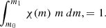 (2)
(2)
Assuming this normalization, FASTAR comes with the six pre-defined functional forms for the IMF. Their basic properties are as follows:
2.1.1. Milky Way-like IMFs.
SSP models with a Milky Way-like IMF can be synthesized assuming either a Kroupa (2001) or a Chabrier (2003) functional form. For these IMFs, only the low-mass and high-mass integration limits of Eq. (2) can be treated as a variable parameter.
2.1.2. Single power-law.
This is a generalization of the Salpeter (1955) IMF1 where the main free parameter is the linear slope α which in FASTAR has a default, Salpeter-like value of 2.35.
2.1.3. Broken power-law.
A three-segment IMF parameterization as implemented in the Conroy & van Dokkum (2012) models. This parameterization is determined by two breaking masses (default mbreak1 = 0.5 and mbreak2 = 1.0) and three slopes connecting them (default α1 = 1.3 representing the low-mass end, α2 = 1.8, and α3 = 2.3 corresponding to the high-mass end slope up to the integration limit).
2.1.4. Bimodal IMF.
The same functional form of the MILES models as defined in Vazdekis et al. (1996) with the high-mass end slope αB as single free parameter with a default value of αB = 2.3. Note that, in contrast to the standard definition of this IMF in the MILES framework, FASTAR describes the IMF in linear units. Thus, the default value for the bimodal IMF mimics a Kroupa-like IMF and corresponds to ΓB = 1.3 in the original notation of the MILES models. Our implementation also allows for a variable low-mass end slope βB (the default value adopted in the MILES models is βB = 1).
2.1.5. Tapered power-law.
We follow the IMF parameterization presented in De Marchi et al. (2005), with a peak mass mp, a high-mass end slope α and a tapering exponent β for the low-mass end. This functional form is particularly flexible and naturally captures any potential characteristic mass of the IMF, providing a direct link to theoretical predictions. The default values are α = β = 2.3 and mp = 0.5 M⊙.
Figure 1 summarizes and compares all these functional forms. In addition, an important asset of FASTAR is that it can also synthesize models with arbitrary, user-defined IMF parameterizations. Examples and guidelines for implementing new IMF functional forms are included in the documentation.
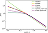 |
Fig. 1. IMF functional forms. FASTAR comes with the six pre-defined IMF parameterizations shown here. All of their parameters can be changed to synthesize new models with variable IMFs. In addition, models for any arbitrary IMF defined by the user can also be calculated. |
2.2. Isochrones and bolometric corrections
FASTAR is based on the most updated version of the BaSTI set of isochrones (Hidalgo et al. 2018; Pietrinferni et al. 2021, 2024). Specifically, FASTAR makes use of the solar-scaled predictions, with improved treatment of atomic diffusion and overshooting beyond the Schwarzschild limit. This choice of isochrones in combination with the stellar libraries (see details below) sets the limits of the FASTAR predictions, which are limited to ages between 20 Myr and 14 Gyr and total metallicities between −2.5 ≥ [M/H]≤ + 0.3. For an extended discussion of the isochrone behavior we refer the reader to Hidalgo et al. (2018).
It is worth noting that, while the isochrones are calculated for a solar-scaled elemental mixture ([α/Fe] = 0), individual stellar templates might have non-solar abundances. In practice, this means that in the synthesis of the FASTAR models based on Eq. (1), we made the common assumption that the [Fe/H] measured for the individual stars approximately corresponds to their total metallicity [M/H]. Because of that, the FASTAR models should be regards as base models, according to the nomenclature in the MILES models’ papers. Details on the implications of this assumption can be found in Vazdekis et al. (2010, 2015).
To provide continuous and differentiable SSP predictions requires the interpolation of the isochrone predictions and given the complexity of stellar evolution physics this can be a particularly challenging task (Dotter 2016). Thankfully, BaSTI isochrones have been intentionally computed to maintain the same number of stellar masses for any age and chemical composition. This greatly simplifies the synthesis as they can be arranged in a regular grid and then linearly interpolated, as implemented in FASTAR.
In addition, as noted above, FASTAR makes use of empirical bolometric corrections to project the theoretical isochrone predictions for the bolometric luminosities into V-band magnitudes directly measurable in the individual stellar templates. FASTAR relies on the V-band bolometric corrections of Worthey & Lee (2011) for all stellar types and metallicities. These predictions are also shaped into a regular grid and then can be linearly interpolated at any desired value of Teff, log g, and [Fe/H].
2.3. Stellar libraries
FASTAR is built around the Medium-resolution Isaac Newton Telescope library of empirical spectra (MILES) (Sánchez-Blázquez et al. 2006). In short, MILES is a compilation of 985 empirical stellar spectra at a spectral resolution of 2.51 Å (Falcón-Barroso et al. 2011) covering a wide range of atmospheric parameters (e.g. from ∼ − 2.5 to ∼ + 0.5 in [Fe/H], including templates as hot as Teff ∼ 25 000 K). With an exquisite flux calibration over the entire 3540–7400 Å wavelength range (down to the ∼2% level), MILES feeds many state-of-the-art SSP models currently available.
While the MILES stellar library provides excellent performance for detailed spectroscopic measurements, photometric analyses usually require combining filters that lie blueward and redward of the MILES wavelength limits. Therefore, FASTAR also makes use of the last version of the BOSZ synthetic stellar spectral library presented in Mészáros et al. (2024). This theoretical library has predictions over a much broader wavelength range (from 100 nm to 32 μm) while simultaneously offering an atmospheric parameter coverage similar to that of MILES (although their predictions are limited to stars cooler than 16 000 K). To be consistent with the FASTAR assumptions, we only make use of the Mészáros et al. (2024) predictions for [α/Fe] = 0 assuming a microturbulent velocity of vmicro = 2 km s−1. With these additional constraints, our final theoretical library is composed of 6151 individual stellar spectra. Details on how these two libraries are combined are provided in the following sections.
2.4. Spectral interpolation
The interpolation of stellar spectra is arguably the central component of evolutionary stellar population synthesis codes. The goal is to predict the spectrum of a star given its Teff, log g, and [Fe/H] and current state-of-the-art models follow two main interpolation approaches. Local interpolators use stellar templates close to the desired (Teff, log g, [Fe/H]) in order to predict the output spectra (e.g., Vazdekis et al. 2003; Sharma et al. 2016). On the contrary, global interpolators parametrize the behavior of the stellar library through high-order polynomial fits in order to synthesize new stellar spectra (e.g., Prugniel et al. 2011; Villaume et al. 2017).
FASTAR implements an alternative, machine learning-powered algorithm that is fast and numerically differentiable. While sophisticated spectral interpolators based on large datasets have been recently explored (e.g., Melchior et al. 2023; Koblischke & Bovy 2024), FASTAR follows the simple yet effective approach presented in Alsing et al. (2020). In short, we first reduce the dimensionality of the stellar libraries using a principal component analysis (PCA) decomposition. Then, a fully connected neural network is used to estimate the mapping between the PCA coefficients and the stellar parameters (Teff, log g, [Fe/H]).
The workflow is as follows. We first convolve the Mészáros et al. (2024) stellar library to match the resolution and wavelength sampling of the MILES templates (Falcón-Barroso et al. 2011). Then, we augment ten times each star within the MILES library using a simple linear interpolation. The augmentation process is rather insensitive to the interpolation scheme since we are only perturbing the spectra within the typical uncertainty of the atmospheric parameters, and allows us to bias the solution toward the empirical spectra in those regions where MILES stellar templates are available.
Equipped with theoretical and the (augmented) empirical templates, we then use a PCA decomposition to reduce the dimensionality of the spectra. In the same line as previous works (e.g., Yip et al. 2004; Portillo et al. 2020; Sharbaf et al. 2023; Iglesias-Navarro et al. 2024, 2025), we find that a relatively small number of components is enough to accurately model our stellar templates. After testing a range of values, we settle on 16 principal components for our analysis. Prior to the PCA, each spectrum is first normalized by its own mean flux and then centered by subtracting the mean spectrum of the entire training set. This procedure removes global flux-level differences and provides stable, zero-centered inputs for the PCA decomposition. Finally, we train a fully connected neural network with four hidden layers (64, 128, 128, 64 neurons) using a mean squared error loss to predict the 16 principal component coefficients of the spectra from the stellar atmospheric parameters (log g, Teff, [Fe/H]). During the training, empirical and stellar templates are used indistinguishably to calculate the loss, with no specific merging strategy. Once trained for 1200 epochs on a standard GPU, the regressor maps stellar parameters to PCA coefficients, which can subsequently be transformed back into full spectra through the PCA basis. Note that, given the limited number of stellar templates available and their sparsity, all of them are used during training.
Figure 2 summarizes the performance of the FASTAR spectral interpolation, with stars in the training set color coded by the reconstruction error measured as the standard deviation of the residuals between original and reconstructed spectra. The typical reconstruction error is on the order of a few percent ( ) and the 99th percentile remains around 10%. Moreover, stellar predictions remain robust across the whole parameter space, only becoming progressively less accurate for the coolest stars. To improve the convergence of the interpolation at these edges, we removed from the training sample theoretical stars cooler than log Teff = 3.5, as well as the most extreme dwarf (log g > 5) and giant (log g < 0) stars, whose spectra are dominated by broad molecular lines and therefore prone to model systematics. No additional calibration was needed to combine the spectra and atmospheric parameters of MILES and BOSZ, revealing a robust consistency in the atmospheric of both libraries. Table 1 summarizes the final training sets.
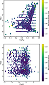 |
Fig. 2. Performance of the FASTAR interpolator across the log g-Teff-[Fe/H] parameter space. Each star in the MILES and BOSZ libraries is color coded by the reconstruction error, defined as the standard deviation of the residuals between the real spectrum and the predicted one. The top panel shows the log g-Teff, while the bottom one shows log g-[Fe/H]. The average error is on the order of ∼3%, only becoming closer to ∼10% for the coolest stars in the sample. There is no significant trend with metallicity. |
Stellar libraries used for the training.
Fig. 3 shows how the FASTAR interpolator compares with the state-of-the-art local interpolation powering the MILES SSP models. Specifically, it shows the combined residual distribution after predicting the spectra of each star in the MILES stellar library. In general, the behavior of both interpolators is similar although FASTAR residuals exhibit less pronounced tails toward extreme outliers. The error due to the PCA dimensionality reduction is shown in gray. Our tests show that beyond 16 components, the uncertainty in the prediction is dominated by the error associated the neural network training and increasing the number of PCA does not lead to better results.
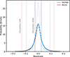 |
Fig. 3. Comparison of residuals. Blue and orange lines represent the distribution of residuals for the FASTAR and MILES interpolators when predicting the stellar spectra of the MILES library. The behavior of both interpolation schemes is similar, as shown by the vertical dashed lines marking the 20th and 80th percentiles. However, the 2nd and 98th percentile vertical lines indicate that extreme errors are less common in FASTAR. For comparison, the gray histogram shows the error associated to the PCA compression. |
Although Fig. 3 showcases the overall behavior of the FASTAR interpolation, stellar population properties are encoded in specific spectral regions and scales. To exemplify the reliability of FASTAR in reproducing these features, Fig. 4 contains four panels, each of them showing in blue how the FASTAR predictions compare to observed colors and line-strengths in the MILES stellar library. For comparison, Fig. 4 also includes the predicted values from the MILES stellar interpolator (orange), as well as the R2 value for each interpolator.
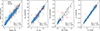 |
Fig. 4. Line-strength and color comparison. Observed (horizontal axes) line-strength and colors are compared to the predicted values (vertical axes) using the FASTAR (blue filled circles) and MILES (orange squares) interpolators. From left to right, we show the behavior of the metallicity-sensitive [MgFe]’ (Thomas et al. 2003), the age-sensitive HβO (Cervantes & Vazdekis 2009), and the IMF-sensitive TiO2 (Faber et al. 1985; Trager et al. 1998). The panel on the right shows the comparison of the (g − r) color. The interpolation in FASTAR tends to outperform that of MILES, with systematically smaller residuals as indicated on the bottom right corner of each panel. |
In general, FASTAR performs systematically better than the MILES interpolator at predicting MILES stellar templates, with smaller residuals for all indices and colors and fewer outliers. Only for the [MgFe]’ line-strength the performance of both interpolators is similar, with some non-linearity apparent in the FASTAR predictions likely due to the difference in [Mg/Fe] between empirical and theoretical libraries (Milone et al. 2011; Mészáros et al. 2024). In this regard, it is worth noting that FASTAR has been trained to reproduce both MILES and BOSZ libraries, while the MILES interpolator is optimized to predict MILES stars. For completeness, in Appendix A we include a more comprehensive comparison between FASTAR and MILES, including a larger set of indices.
3. Model synthesis
The evolutionary synthesis of FASTAR is completely defined by the ingredients listed above. The main outcome of FASTAR, i.e., the spectroscopic and photometric predictions are exemplified in Fig. 5 showing the spectral energy distribution expected for an old (10 Gyr), solar metallicity ([M/H] = 0) integrated stellar population. The normalization of the FASTAR prediction is anchored to an assumed absolute bolometric magnitude of the Sun of 4.70 and a bolometric correction of BC⊙ = −0.12. With this, the units of the predicted fluxes Fλ are erg s−1 cm−2 Å−1, scaled at 10 pc, making the computation of absolute magnitudes in any photometric band straightforward.
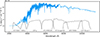 |
Fig. 5. FASTAR spectroscopic and photometric predictions. Blue lines show to the FASTAR SSP models for a 10 Gyr old, solar metallicity population. In light blue, the FASTAR photometric model is based on the BOSZ theoretical stellar library and can be convolved with any set of photometric filters (exemplified by the different transmission functions in grey) to generate photometric predictions. In addition, the spectroscopic side of FASTAR (dark blue line) combines the MILES (empirical) and BOSZ stellar libraries to generate models oriented toward detailed stellar population analyses. |
Note that the synthesis of FASTAR, including all its ingredients and operations, is entirely coded using the JAX Python library (Bradbury et al. 2018; Frostig et al. 2019), allowing for a optimized computation in both CPU and GPU and native numerical autodifferentiation. The scope of this paper is, however, to describe the evolutionary aspects of the FASTAR synthesis, not its technical implementation. For a more in-depth description of the advantages of JAX in the analysis of stellar populations, we refer the reader to the recent overview presented in Hearin et al. (2023).
FASTAR provides two set of consistent predictions. On the one hand, spectroscopic SSP models can be calculated for any age and metallicity within the isochrone range, combining the MILES empirical stellar library and the theoretical stellar spectra of BOSZ. These spectroscopic FASTAR models are generated at a resolution of 2.51 Å over the MILES wavelength range 3525–7500 Å and shown in Fig. 5 as a dark blue line. On the other hand, FASTAR can also be used for photometric analyses over a wider wavelength range (2000–11 500 Å) based solely on the BOSZ theoretical spectra (light blue line in Fig. 5). This photometric version of FASTAR is at the same resolution as the spectroscopic one but intentionally undersampled (Δλ = 4 Å) to strongly discourage its use for spectroscopic applications. Note that this wavelength range is narrower than what is in principle allowed by the BOSZ templates, focusing only on those wavelengths commonly covered by optical photometric filters.
3.1. Line-strengths and colors
Figure 6 presents the FASTAR SSP predictions for the HβO, Mgb, and TiO2 as a function of age, metallicity and IMF slope, respectively. For comparison, Fig. 6 also includes the MILES predictions for the same set of line-strength indices. In all cases, indices have been measured at the nominal 2.51 Å resolution.
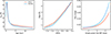 |
Fig. 6. Line-strength comparison. Blue and orange lines indicate, respectively, the FASTAR and MILES predictions for different line-strength indices at a 2.51 Å resolution. Left panel: Equivalent width of the HβO line is shown as a function of age for a population of solar metallicity and a Milky Way-like IMF. For old ages, FASTAR predictions tend to be lower than those of MILES. Middle panel: dependence of the Mgb feature on metallicity for a 10 Gyr population with a Milky Way-like IMF. Right panel: Behavior of the TiO2 molecular band for different IMF slope values (single power law) is shown for 10 Gyr and solar metallicity population. |
In general, FASTAR predictions follow the expectations for state-of-the-art stellar population synthesis models. Given the similarities in the line-strength measured for the individual stars shown in Fig. 4, the differences between FASTAR and MILES arise from the different choice of isochrones and bolometric corrections. Two important differences are worth mentioning. In the top panel of Fig. 6, FASTAR predicts lower HβO values than MILES for old stellar populations. These low HβO values in FASTAR would tend to alleviate the long-standing zero-point issue of evolutionary stellar population models (see e.g., Gibson et al. 1999; Vazdekis et al. 2001; Schiavon et al. 2002; Mendel et al. 2007; Cenarro et al. 2008; Percival & Salaris 2009; La Barbera et al. 2013; Leath et al. 2022). Secondly, the bottom panel of Fig. 6 shows that FASTAR tends to predict higher TiO2 equivalent widths than MILES for high IMF slope values. This results from the differences in the TiO2 behavior at low effective temperature between the MILES and BOSZ libraries, as demonstrated in Appendix B. It is important to acknowledge that the modeling of these prominent molecular features is particularly challenging, potentially affecting both the theoretical synthesis of stellar templates and the determination of atmospheric parameters in empirical libraries. For completeness, Appendix C includes a more extended comparison between FASTAR and MILES for a large set of widely used line-strength indices.
Similarly, in Fig. 7 we show the (g − r) color dependence on age, metallicity and IMF slope for FASTAR, using both the photometric and the spectroscopic synthesizer, as well as the comparison with MILES. The three predictions are in overall agreement, with no significant differences between photometric and spectroscopic FASTAR models. The (g − r) dependence on the IMF is also sensitive to the model ingredients. As in Fig. 6, FASTAR tends to show milder changes in color than MILES when increasing the IMF slope value (i.e. the number of low-mass stars). In addition, the photometric FASTAR predictions show an even weaker dependence on the IMF. Given the prominence of broad molecular bands in the atmospheres of cool stars, the differences between the two FASTAR predictions (solid and dashed blue lines in the bottom panel of Fig. 7) are expected to be related to the theoretical versus empirical modelling of these molecular bands.
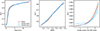 |
Fig. 7. Color predictions. From left to right, each panel shows the color sensitivity of the photometric and spectroscopic FASTAR models (dashed and solid blue lines, respectively), as well as the MILES predictions (in orange) for comparison. The differences between the three models are due to the use of theoretical versus empirical stellar libraries and the choice of bolometric corrections (between FASTAR and MILES). The assumed ages, metallicities and IMF slopes are the same as in Fig. 6. |
3.2. Magnitudes and mass-to-light ratios
Magnitudes and mass-to-light ratios can also be readily calculated within FASTAR. As indicated above, FASTAR predictions are scaled so that the absolute magnitude of any given SSP model is straightforward to compute. In practice, given a generic photometric filter P, FASTAR fluxes Fλ (from Eq. (1)) can be translated into absolute AB magnitudes through the following equation:
 (3)
(3)
with the average flux density ⟨Fλ⟩P within the filter given by:
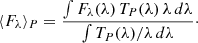 (4)
(4)
In the equation above, Fλ is the predicted FASTAR spectrum, TP(λ) the transmission function of the filter, and λ the wavelength array (in Å). In short, because of the units and scaling of FASTAR, Eq. (3) predicts the absolute AB magnitude of a stellar population that formed 1 solar mass at birth.
In addition to this, FASTAR can also provide the expected mass-to-light ratio in any photometric filter within the predicted wavelength range (∼3900–7000 Å for spectroscopic FASTAR and 2000-to-12 000 Å for the photometry-oriented models). These mass-to-light ratios are calculated using the CALSPEC Kurucz model of the Sun (Bohlin et al. 2014), scaled to our assumed V-band absolute magnitude (see Sect. 3).
FASTAR provides two different mass-to-light ratio M/L predictions. The most directly connected to the stellar population content of galaxies is the stellar M/L. This stellar M/L is defined as the stellar mass of the population (in M⊙ units) divided by its luminosity (also in solar units). However, there are situations where it might be useful to estimate the total mass of a system given its stellar luminosity, including not only the mass in stars but also the mass in stellar remnants and the mass in form of gas ejected by stellar winds. For these cases, FASTAR also provides a total M/L that takes into account all mass sources. If one wants to translate the observed luminosity of a galaxy into a stellar mass, one might use the stellar M/L since the use of the total M/L requires further assumptions (i.e. knowing the behavior of the high mass end of the IMF even if those stars are not present or the assumption that all stellar remnants and gas remain within the observed region or galaxy.)
To illustrate the FASTAR magnitudes and M/L predictions, Fig. 8 shows their dependence on the age, metallicity and IMF slope of the underlying population for two different photometric filters, one in the optical and one in the near-infrared. In this case, the mass-to-light ratio corresponds to the stellar ones. Trends are as expected, with higher M/L ratios for older, more metal rich, and bottom-heavier IMF slopes. The brightness of the SSP models increase with decreasing age and metallicities, more significantly in the optical range (green lines). Interestingly, for old ages and solar metallicities, the expected brightness of a population has a minimum for an IMF slope similar to that of the Milky Way.
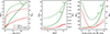 |
Fig. 8. Mass-to-light ratio and magnitude trends. Solid lines and left vertical axes represent the change in stellar M/L as a function of age (left), metallicity (middle), and IMF slope (right). When not varied, the age is fixed to 10 Gyr, the metallicity to solar, and the IMF to the Milky Way value. Similarly, dashed lines and right axes correspond to the expected absolute magnitude of the population. FASTAR predictions for the SDSS g band are shown in green while the expectation for the near-infrared JWST/NIRCam F090W filter are shown in red. |
3.3. FASTAR unique features
Spectra and the derived line-strength values, colors and M/L are all standard outputs of evolutionary stellar population synthesis models. With FASTAR, however, it is possible to go beyond these standard predictions. The differentiable and continuous nature of FASTAR can be used, not only to implement more sophisticated gradient-based inversion algorithms, but also to achieve a deeper understanding of SSP models. For example, in the left panel of Fig. 9 we show the partial derivative of an SSP model with respect to its age (at solar metallicity). This left panel formalizes the well-known idea that changes in the age have progressively less effect on the integrated spectrum of a galaxy as age increases. In simple terms, distinguishing a 1 Gyr difference is much easier for younger than for older populations. Interestingly, the maximum contribution of AGN and RGB stars to the integrated spectra is also evident as a clear peak in the derivative of the flux at ∼1.5 Gyr.
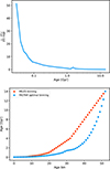 |
Fig. 9. Optimal age sampling. Top: Relative age sensitivity of FASTAR SSP models as a function of age. The normalized age derivative of the FASTAR models becomes smaller for older ages, reflecting the fact that age variations have a progressively weaker effect on the integrated spectrum of a galaxy with increasing age. The peak contribution of the AGB (and RGB) phases appears as a sudden change in the derivative at an age of ∼1.5 Gyr. Bottom: Age sampling of the MILES models is shown in red, following their BaSTI isochrone grid. In blue, the optimized FASTAR sampling enforces a constant flux variation across all age bins. |
This robust quantification of the age gradient can be used in practice to improve upon current SSP modelling. Specifically, SSP model predictions are computed in an age grid following the sampling given by the isochrones, as exemplified by the red symbols on the right panel of Fig. 9. This age sampling aims to roughly capture the change in age sensitivity represented in the left panel, with older SSP having a coarser sampling than younger ones. With FASTAR we can formally create an optimal grid of models that ensures that the relative variation of the spectra is the same between two consecutive SSP models, as showcased by the blue symbols on the right panel of Fig. 9. The optimal age sampling also captures the sudden contribution of giant stars to the integrated flux of SSP models.
With FASTAR we provide an optimized age and metallicity sampling based on the mean variation of the spectra. In addition, the sampling can be easily optimized for any other metric (e.g. magnitude in a specific band, lines-strength, color etc.) thanks to the differentiable nature of the model predictions. The documentation released with the code includes examples on how to optimize the sampling for alternative quantities.
In addition, the computation speed of FASTAR can be used to estimate the uncertainty of our spectral and photometric predictions, as illustrated in Fig. 10. The top panel shows a standard SSP model of an old (10 Gyr), solar metallicity integrated population. On the bottom panel we show four error spectra calculated as follows. The purple one corresponds to the standard deviation of 100 SSP realizations where the surface gravity of each star along the isochrone was perturbed following a gaussian distribution with dispersion Δlog g = 0.2 dex. In other words, it corresponds to the error in the SSP prediction resulting from the typical uncertainty in the determination of log g in the individual stellar templates. Similarly, the red line shows the error resulting from propagating a typical stellar metallicity uncertainty of Δ[Fe/H] = 0.1 dex. Finally, with yellow we indicate the uncertainty related to the determination of the effective temperature (ΔlogTeff = 0.005 dex). The gray line correspond to the total error budget, calculated by simultaneously perturbing the three atmospheric parameters.
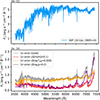 |
Fig. 10. Uncertainty of SSP model predictions. The upper panel shows the SSP model predicted by FASTAR for a population of 10 Gyr and solar metallicity while the bottom panel shows the associated errors. In purple, we present the uncertainty in the SSP model assuming a typical error Δlog g = 0.2 dex in the determination of the surface gravity of the stars. In red and yellow we represent the error corresponding to the metallicity (Δ[Fe/H] = 0.1 dex) and effective temperature (ΔTeff = 0.005 dex), respectively. In grey, we show the expected total uncertainty in the SSP model. |
With these assumptions, the SSP prediction shown in the upper panel has, on average, a signal-to-noise ratio ∼600 around λ = 5000, slightly lower (∼300) toward the blue and the red ends of the optical range. Interestingly, the dominant source of uncertainty across the entire wavelength range is related to the error in the determination of the effective temperature of individual stars. It is worth noting, however, that this is an approximate estimate, assuming constant, uncorrelated and gaussian errors. Moreover, the current version of FASTAR does not take into account the PCA reconstruction loss nor the epistemic uncertainty of the neural network predictions, which will be implemented in upcoming releases. Nonetheless, Fig. 10 showcases the possibilities of using FASTAR to better understand the strengths and limitations of SSP models.
3.4. Stellar predictions
The prediction of stellar templates is implicit to the calculation of SSP models through the neural network-based interpolation scheme described above. To facilitate its usage for scientific cases where individual stellar templates might be required, FASTAR also makes straightforward and fast to predict new stellar spectra. After fixing the metallicity, effective temperature and surface gravity, FASTAR generates stellar predictions across the two (spectroscopic and photometric) wavelength ranges. This is exemplified in Fig. 11.
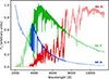 |
Fig. 11. Stellar predictions across different spectral types. Dark and light lines represent predictions using both the MILES and BOSZ stellar libraries, and using only BOSZ, respectively. Each color corresponds to a different stellar type, as indicated by the labels. |
Darker lines in Fig. 11 correspond to the FASTAR predictions within the MILES wavelength range, based on both MILES and BOSZ stellar libraries, while lighter lines are the coarser (in wavelength) FASTAR stellar predictions for photometric applications. Without any fine tuning, the two predictions are in clear agreement.
4. Validation on observed data
Globular clusters and massive quiescent early-type galaxies are observational benchmarks for the performance of evolutionary population synthesis models. Their stellar populations are rather simple and homogeneous and thus well-represented by SSP models.
In Fig. 12 we show the HβO versus [MgFe]’ index-index diagram for the Milky Way globular cluster sample of Usher et al. (2017), color coded by their [Fe/H] metallicity. Figure 12 also shows the FASTAR predictions for different ages and metallicities, assuming a Milky Way-like IMF. The globular cluster indices were measured at the nominal 2.51 Å resolution of the FASTAR models.
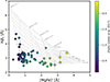 |
Fig. 12. Line-strength HβO versus [MgFe]’ index-index diagram for Milky Way globular clusters. Filled symbols correspond to the globular cluster sample of Usher et al. (2017), color coded by their [Fe/H] metallicity. The FASTAR model grid prediction is shown in the background in grey. Labels indicate ages and metallicities across the grid. The equivalent width for data and models is measured at the FASTAR 2.51 Å spectral resolution. FASTAR model predictions reproduce the observed data without systematic offsets, suggesting that the well-known zero-point problem of evolutionary stellar population models can be at least minimized with state-of-the art isochrones. |
In general, FASTAR predictions reliably match the observed data, with old stellar populations across the entire globular cluster population and the independently measured metallicities (i.e. the color code in Fig. 12) running in parallel with the iso-metallicity lines of the FASTAR models. Beyond this agreement, the most notable aspect of this comparison is the lack of a significant zero-point difference between models and data, with the fit to the oldest globular clusters in the sample not requiring ages older than 14 Gyr (i.e. the age of the Universe at z ∼ 0 under standard cosmologies). Interestingly, this well-known systematic of evolutionary synthesis models is present in the MILES models (see e.g., Leath et al. 2022) but not in FASTAR, where the predicted HβO values tend to be smaller for the same age (see Fig. 4). Given the similarities between the MILES and FASTAR stellar line-strength predictions (Fig. 6), the apparent lack of discrepancy between FASTAR models and globular cluster data is due to the improved stellar evolutionary physics in the Hidalgo et al. (2018) set of isochrones, in particular, thanks to the treatment of atomic diffusion.
The comparison with observed globular cluster data can be extended beyond the Milky Way. To showcase the broad range of applications of the FASTAR models, Fig. 13 shows the (g − z) versus [MgFe]’ model grid prediction for a Milky Way-like IMF. On top of the model grid, filled circles correspond to the globular cluster sample of Fahrion et al. (2020) in the Fornax cluster, color coded by their total metallicity. Observationally, measuring colors and line-strengths in globular clusters is significantly more difficult in external galaxies than in the Milky Way, in addition to the effect of non-solar elemental abundances, thus explaining the increased scatter in comparison with Fig. 12. However, the agreement between models and data is noteworthy, particularly considering that the color predictions come from the FASTAR photometric models trained on synthetic stellar spectra, while the [MgFe]’ line-strengths are measured from the spectroscopic models relying on both theoretical and empirical templates.
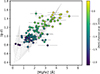 |
Fig. 13. Globular clusters in the Fornax Cluster. Filled circles correspond to the (g − z) versus [MgFe]’ values measured in the Fahrion et al. (2020) sample of globular clusters in the Fornax galaxy cluster, with the color coding representing their total metallicity. The background model grid shows the FASTAR predictions for different ages and metallicities, with the (g − z) and [MgFe]’ values, coming from the FASTAR photometric and spectroscopic sets of predictions, respectively. |
To further benchmark FASTAR predictions against globular cluster measurements, Fig. 14 shows the observed (u − g) versus (g − r) colors of M 31 globular clusters from Caldwell et al. (2011), overplotted on top of a grid of (photometric) FASTAR predictions. The sample of globular clusters has been restricted to those with low attenuation (E(B − V) < 0.15) to minimize the effect of dust. Clusters are color coded according to their [Fe/H] iron metallicities. The agreement between observations and models is good, with a clear trend between the observed colors, models, and metallicities, in particular for the metal-poor population less affected by dust.
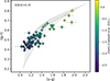 |
Fig. 14. Globular clusters in M 31. The (u − g) versus (g − r) colors of globular clusters in M 31 are shown, color coded by their iron metallicity, as reported in Caldwell et al. (2011). To minimize the effect of dust, the sample has been reduced to those globular clusters with E(B − V) < 0.15. The gray background grid shows the FASTAR photometric predictions for different ages and metallicities, for a fixed Milky Way-like IMF. |
In addition to globular clusters, we also tested the FASTAR models against the high-quality Sloan Digital Sky Survey (SDSS; Adelman-McCarthy et al. 2008) stacked optical spectra of quiescent early-type galaxies presented and described in La Barbera et al. (2013). Figure 15 shows again the HβO–[MgFe]’ plane, compared to line-strengths measured from the SDSS stacked spectra, color coded by stellar velocity dispersion σ. Indices are measured at the spectral resolution given by the stacked spectra with the highest velocity dispersion. As expected, FASTAR models predict a clear age and metallicity dependence with velocity dispersion, with galaxies having higher σ presenting older and more metal-rich stellar populations. The recovered comparison is rather similar to the analysis presented in La Barbera et al. (2013) using the MILES models.
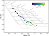 |
Fig. 15. Ages and metallicities of quiescent early-type galaxies. Filled symbols correspond to the HβO and [MgFe]’ line-strength measured over the stacked SDSS spectra of La Barbera et al. (2013), with the color code given by the mean stellar velocity dispersion of each stack. The background model grid shows the FASTAR predictions for those two indices for a Milky Way IMF (solid lines). For reference, the grid for a bottom-heavy IMF (single power law with α = 3) is also shown with dashed lines. As expected, the prediction from the FASTAR models is that quiescent early-type galaxies become increasingly more metal-rich and older when increasing velocity dispersion. Models and data have been convolved to the resolution of the highest σ stack. |
Contrary to globular clusters, the oldest and most massive galaxies in Fig. 15 appear systematically below the HβO prediction for the 14 Gyr SSP. However, this is not necessarily due to a model zero-point issue but to the effect on HβO of a bottom-heavy IMF (i.e., biased toward low-mass stars, La Barbera et al. 2013), as well as individual elemental abundance variations. For comparison, Fig. 15 also includes, with dashed lines, a FASTAR grid assuming bottom-heavy IMF.
Figure 16 offers a more quantitative assessment of the performance of FASTAR in comparison with the state-of-the-art MILES evolutionary synthesis models. We use pPXF (Cappellari & Emsellem 2004; Cappellari 2023) to fit the SDSS stacked spectra using both sets of models. In the case of FASTAR, we adopt the optimized age-metallicity sampling described in Sect. 3.3, while fits based on MILES use the default MILES grid. The fits include templates for potential (although weak) emission lines and are done with no continuum correction to avoid compensating potential model systematics. No regularization was applied either, and we masked the NaD region during the fitting process to mitigate the effect of IMF variations and neutral gas absorption.
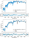 |
Fig. 16. Fits to SDSS stacked spectra. The MILES (in orange) and FASTAR (in blue) best-fitting models are shown compared to two SDSS stacked spectra (in black). The top and bottom panels correspond to stacks of low-σ (110 km s−1) and high-σ (280 km s−1) early-type galaxies, respectively. MILES and FASTAR best-fitting models are very similar as demonstrated by the residual distribution also displayed in each panel. No polynomial correction was applied to the continuum. |
For both the low- and high-σ stacked spectra, the FASTAR and MILES solutions provide very good fits to the data, with residuals below the 5% level in both cases. This is particularly noteworthy since no polynomial correction is included to account for flux calibration mismatches in the SDSS data. In the case of the high-σ stack, the residuals are in both cases slightly larger, likely due to non-solar elemental abundances in the underlying stellar population and a bottom-heavy IMF.
In Figs. 17 and 18 we show the recovered age – velocity dispersion and metallicity – velocity dispersion relations, respectively. As before, blue symbols correspond to measurements obtained using the FASTAR models and orange ones correspond to MILES. In both figures, filled symbols are mass-weighted quantities while empty symbols represent luminosity-weighted averages. Generally, FASTAR and MILES models behave similarly, retrieving the well-known trend of older and more metal-rich stellar populations with increasing galaxy velocity dispersion.
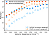 |
Fig. 17. Age-velocity dispersion relation. Blue and orange symbols correspond to the best-fitting ages of the SDSS stacked spectra using pPXF and the FASTAR and MILES SSP models, respectively, while filled and empty symbols indicate mass- and luminosity-weighted values. FASTAR and MILES models are able to retrieve the expected age-σ relation, with FASTAR-based ages generally being younger than those measured with MILES. |
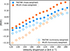 |
Fig. 18. Metallicity-velocity dispersion relation. The symbols and colors are the same as in Fig. 17, but in this case they represent the best-fitting metallicity values. The expected relation with velocity dispersion is well recovered with both sets of models although with systematic differences as FASTAR tends to result in lower metallicities and less differences between mass-weighted and luminosity-weighted values than MILES. |
FASTAR tends to retrieve younger ages (Fig. 17), as expected from the line-strength behavior detailed above, with weaker HβO values at fixed age than in MILES. Interestingly, age-σ relation measured with the FASTAR model shows a peculiar behavior at σ ∼ 200 km s−1, which is also evident in the HβO–[MgFe]’ plane shown in Fig. 15 but apparently absent when using the MILES models. Regarding the recovered metallicities, FASTAR-based measurements show smaller differences between luminosity- and mass-weighted trends compared to MILES, with systematically lower mass-weighted values.
5. Summary
With FASTAR we present the first generation of continuous, differentiable evolutionary stellar population synthesis algorithms. FASTAR is not a set of pre-computed model predictions, but a flexible tool that provides continuous SSP predictions across a wide range of ages, metallicities, IMFs and wavelengths. Based on the fundamental principles of evolutionary stellar population models, FASTAR, however, is faster and enables a deeper understanding of the models’ behavior and new ways of using their thoroughly tested strengths. The access to the synthesis code is transparent and allows users to tailor FASTAR predictions to their needs. The key features of FASTAR are as follows:
-
PCA-based, neural network stellar interpolation. FASTAR is centered around a stellar interpolator trained on empirical and/or theoretical stellar libraries that matches the reliability of competing interpolation schemes currently implemented in SSP models, but it is faster and matches the performance of state-of-the-art alternatives in accurately reproducing stellar spectra.
-
Differentiability and flexibility. FASTAR uses the JAX numerical library to provide differentiable SSP predictions, ready to be implemented in gradient descent inference algorithms. Moreover, it allows for the use of any IMF functional form, facilitating the cross-IMF conversions of colors, stellar masses and all other model predictions.
-
Age and metallicity coverage. FASTAR relies on the latest version of the BaSTI-IAC set of isochrones, thus enabling SSP predictions from 20 Myr to 14 Gyr in age and from −2.5 to +0.3 in total metallicity. Possible IMF slopes and functional forms are completely unconstrained.
-
Detailed spectroscopy. Over the 35 400–7400 Å wavelength range, FASTAR offers detailed stellar and SSP predictions at a 2.51Å resolution. The code combines the MILES (empirical) and BOSZ (theoretical) stellar libraries to deliver detailed SSP predictions. Colors, magnitudes, mass-to-light ratios, line-strengths etc. can be easily computed as well.
-
Photometric predictions. For photometric applications, FASTAR offers a wider wavelength range, from 2000 Å to 12 000 Å using the BOSZ theoretical stellar library. The resulting SEDs can then be convolved with any photometric filter and the corresponding colors and mass-to-light ratios can be consistently estimated.
-
Unique to FASTAR. FASTAR proposes an alternative way of releasing SSP models. Predictions can be evaluated at any age, metallicity or IMF. In addition, FASTAR provides an optimal age and metallicity grid sampling based on the formal flux derivative of the models. FASTAR can also be used to assess the intrinsic uncertainty of SSP predictions.
Data availability
Documentation and examples on how to use FASTAR can be found at the project’s website https://fastar.readthedocs.io
The code is freely available here https://github.com/inavarro/fastar
Acknowledgments
We would like to thank the referee for the suggestions and comments on the original manuscript. We acknowledge support from grant PID2022-140869NB-I00 from the Spanish Ministry of Science and Innovation. F.L.B. acknowledges support from INAF minigrant 1.05.23.04.01. We would like to thank Ignacio Ferreras, Sebastián Hidalgo, Ignacio Trujillo and Francesco Belfiore for their insightful comments during the development of FASTAR.
References
- Acquaviva, V., Gawiser, E., & Guaita, L. 2011, ApJ, 737, 47 [NASA ADS] [CrossRef] [Google Scholar]
- Adelman-McCarthy, J. K., Agüeros, M. A., Allam, S. S., et al. 2008, ApJS, 175, 297 [NASA ADS] [CrossRef] [Google Scholar]
- Alsing, J., Peiris, H., Leja, J., et al. 2020, ApJS, 249, 5 [CrossRef] [Google Scholar]
- Alsing, J., Thorp, S., Deger, S., et al. 2024, ApJS, 274, 12 [NASA ADS] [CrossRef] [Google Scholar]
- Angthopo, J., Granett, B. R., La Barbera, F., et al. 2024, A&A, 690, A198 [NASA ADS] [CrossRef] [EDP Sciences] [Google Scholar]
- Asa’d, R. S., Vazdekis, A., Cerviño, M., et al. 2017, MNRAS, 471, 3599 [CrossRef] [Google Scholar]
- Behroozi, P. S., Wechsler, R. H., & Conroy, C. 2013, ApJ, 770, 57 [NASA ADS] [CrossRef] [Google Scholar]
- Bellstedt, S., & Robotham, A. S. G. 2025, MNRAS, 540, 2703 [Google Scholar]
- Bohlin, R. C., Gordon, K. D., & Tremblay, P. E. 2014, PASP, 126, 711 [NASA ADS] [Google Scholar]
- Bradbury, J., Frostig, R., Hawkins, P., et al. 2018, JAX: Composable Transformations of Python+NumPy Programs [Google Scholar]
- Bruzual, G., & Charlot, S. 2003, MNRAS, 344, 1000 [NASA ADS] [CrossRef] [Google Scholar]
- Byrne, C. M., Stanway, E. R., Eldridge, J. J., McSwiney, L., & Townsend, O. T. 2022, MNRAS, 512, 5329 [NASA ADS] [CrossRef] [Google Scholar]
- Caldwell, N., Schiavon, R., Morrison, H., Rose, J. A., & Harding, P. 2011, AJ, 141, 61 [NASA ADS] [CrossRef] [Google Scholar]
- Cappellari, M. 2023, MNRAS, 526, 3273 [NASA ADS] [CrossRef] [Google Scholar]
- Cappellari, M., & Emsellem, E. 2004, PASP, 116, 138 [Google Scholar]
- Carnall, A. C., McLure, R. J., Dunlop, J. S., & Davé, R. 2018, MNRAS, 480, 4379 [Google Scholar]
- Cenarro, A. J., Cardiel, N., Gorgas, J., et al. 2001, MNRAS, 326, 959 [NASA ADS] [CrossRef] [Google Scholar]
- Cenarro, A. J., Cervantes, J. L., Beasley, M. A., Marín-Franch, A., & Vazdekis, A. 2008, ApJ, 689, L29 [NASA ADS] [CrossRef] [Google Scholar]
- Cervantes, J. L., & Vazdekis, A. 2009, MNRAS, 392, 691 [NASA ADS] [CrossRef] [Google Scholar]
- Chabrier, G. 2003, PASP, 115, 763 [Google Scholar]
- Chen, Y.-P., Trager, S. C., Peletier, R. F., et al. 2014, A&A, 565, A117 [NASA ADS] [CrossRef] [EDP Sciences] [Google Scholar]
- Chevallard, J., & Charlot, S. 2016, MNRAS, 462, 1415 [NASA ADS] [CrossRef] [Google Scholar]
- Choi, J., Dotter, A., Conroy, C., et al. 2016, ApJ, 823, 102 [Google Scholar]
- Coelho, P. R. T. 2014, MNRAS, 440, 1027 [Google Scholar]
- Conroy, C. 2013, ARA&A, 51, 393 [NASA ADS] [CrossRef] [Google Scholar]
- Conroy, C., & van Dokkum, P. G. 2012, ApJ, 760, 71 [Google Scholar]
- Conroy, C., Villaume, A., van Dokkum, P. G., & Lind, K. 2018, ApJ, 854, 139 [Google Scholar]
- De Marchi, G., Paresce, F., & Portegies Zwart, S. 2005, Astrophys. Space Sci. Lib., 327, 77 [NASA ADS] [CrossRef] [Google Scholar]
- Dotter, A. 2016, ApJS, 222, 8 [Google Scholar]
- Faber, S. M., Friel, E. D., Burstein, D., & Gaskell, C. M. 1985, ApJS, 57, 711 [NASA ADS] [CrossRef] [Google Scholar]
- Fahrion, K., Lyubenova, M., Hilker, M., et al. 2020, A&A, 637, A27 [NASA ADS] [CrossRef] [EDP Sciences] [Google Scholar]
- Falcón-Barroso, J., Sánchez-Blázquez, P., Vazdekis, A., et al. 2011, A&A, 532, A95 [Google Scholar]
- Frostig, R., Johnson, M. J., & Leary, C. 2019, SysML Conference 2018 (Stanford, United States) [Google Scholar]
- Gallazzi, A., Charlot, S., Brinchmann, J., White, S. D. M., & Tremonti, C. A. 2005, MNRAS, 362, 41 [Google Scholar]
- Gibson, B. K., Madgwick, D. S., Jones, L. A., Da Costa, G. S., & Norris, J. E. 1999, AJ, 118, 1268 [NASA ADS] [CrossRef] [Google Scholar]
- Girardi, L., Bressan, A., Bertelli, G., & Chiosi, C. 2000, A&AS, 141, 371 [NASA ADS] [CrossRef] [EDP Sciences] [Google Scholar]
- Gustafsson, B., Edvardsson, B., Eriksson, K., et al. 2008, A&A, 486, 951 [NASA ADS] [CrossRef] [EDP Sciences] [Google Scholar]
- Hahn, C., & Melchior, P. 2022, ApJ, 938, 11 [NASA ADS] [CrossRef] [Google Scholar]
- Hawcroft, C., Leitherer, C., Aranguré, O., et al. 2025, ApJS, 280, 5 [Google Scholar]
- Hearin, A. P., Chaves-Montero, J., Alarcon, A., Becker, M. R., & Benson, A. 2023, MNRAS, 521, 1741 [NASA ADS] [CrossRef] [Google Scholar]
- Hernández-Pérez, F., & Bruzual, G. 2013, MNRAS, 431, 2612 [CrossRef] [Google Scholar]
- Hidalgo, S. L., Pietrinferni, A., Cassisi, S., et al. 2018, ApJ, 856, 125 [Google Scholar]
- Hunt, L. J., Pimbblet, K. A., & Benoit, D. M. 2024, MNRAS, 529, 479 [CrossRef] [Google Scholar]
- Iglesias-Navarro, P., Huertas-Company, M., Martín-Navarro, I., Knapen, J. H., & Pernet, E. 2024, A&A, 689, A58 [NASA ADS] [CrossRef] [EDP Sciences] [Google Scholar]
- Iglesias-Navarro, P., Huertas-Company, M., Pérez-González, P., et al. 2025, A&A, 703, A229 [NASA ADS] [CrossRef] [EDP Sciences] [Google Scholar]
- Johnson, B. D., Leja, J., Conroy, C., & Speagle, J. S. 2021, ApJS, 254, 22 [NASA ADS] [CrossRef] [Google Scholar]
- Kauffmann, G., Heckman, T. M., White, S. D. M., et al. 2003, MNRAS, 341, 33 [Google Scholar]
- Knowles, A. T., Sansom, A. E., Vazdekis, A., & Allende Prieto, C. 2023, MNRAS, 523, 3450 [NASA ADS] [CrossRef] [Google Scholar]
- Koblischke, N., & Bovy, J. 2024, ArXiv e-prints [arXiv:2411.04750] [Google Scholar]
- Kroupa, P. 2001, MNRAS, 322, 231 [NASA ADS] [CrossRef] [Google Scholar]
- Kroupa, P. 2002, Science, 295, 82 [Google Scholar]
- La Barbera, F., Ferreras, I., Vazdekis, A., et al. 2013, MNRAS, 433, 3017 [Google Scholar]
- Leath, H. J., Beasley, M. A., Vazdekis, A., Salvador-Rusiñol, N., & Gvozdenko, A. 2022, MNRAS, 512, 548 [NASA ADS] [CrossRef] [Google Scholar]
- Leitherer, C., Schaerer, D., Goldader, J. D., et al. 1999, ApJS, 123, 3 [Google Scholar]
- Levesque, E. M., & Leitherer, C. 2013, ApJ, 779, 170 [NASA ADS] [CrossRef] [Google Scholar]
- Liang, Y., Melchior, P., Lu, S., Goulding, A., & Ward, C. 2023, AJ, 166, 75 [NASA ADS] [CrossRef] [Google Scholar]
- Lu, S., Daddi, E., Maraston, C., et al. 2024, Nat. Astron., 9, 128 [Google Scholar]
- Madau, P., & Dickinson, M. 2014, ARA&A, 52, 415 [Google Scholar]
- Maiolino, R., & Mannucci, F. 2019, A&ARv, 27, 3 [Google Scholar]
- Maraston, C. 2005, MNRAS, 362, 799 [NASA ADS] [CrossRef] [Google Scholar]
- Maraston, C., Hill, L., Thomas, D., et al. 2020, MNRAS, 496, 2962 [Google Scholar]
- Martín-Navarro, I., La Barbera, F., Vazdekis, A., Falcón-Barroso, J., & Ferreras, I. 2015, MNRAS, 447, 1033 [Google Scholar]
- Martín-Navarro, I., Lyubenova, M., van de Ven, G., et al. 2019, A&A, 626, A124 [Google Scholar]
- Melchior, P., Liang, Y., Hahn, C., & Goulding, A. 2023, AJ, 166, 74 [NASA ADS] [CrossRef] [Google Scholar]
- Mendel, J. T., Proctor, R. N., & Forbes, D. A. 2007, MNRAS, 379, 1618 [NASA ADS] [CrossRef] [Google Scholar]
- Mészáros, S., Bohlin, R., Allende Prieto, C., et al. 2024, A&A, 688, A197 [NASA ADS] [CrossRef] [EDP Sciences] [Google Scholar]
- Millán-Irigoyen, I., Mollá, M., Cerviño, M., et al. 2021, MNRAS, 506, 4781 [CrossRef] [Google Scholar]
- Milone, A. D. C., Sansom, A. E., & Sánchez-Blázquez, P. 2011, MNRAS, 414, 1227 [NASA ADS] [CrossRef] [Google Scholar]
- Parikh, T., Thomas, D., Maraston, C., et al. 2018, MNRAS, 477, 3954 [Google Scholar]
- Peletier, R. F. 1989, Ph.D. Thesis, University of Groningen, The Netherlands [Google Scholar]
- Peng, Y.-J., Lilly, S. J., Kovač, K., et al. 2010, ApJ, 721, 193 [Google Scholar]
- Percival, S. M., & Salaris, M. 2009, ApJ, 703, 1123 [Google Scholar]
- Pietrinferni, A., Cassisi, S., Salaris, M., & Castelli, F. 2004, ApJ, 612, 168 [Google Scholar]
- Pietrinferni, A., Cassisi, S., Salaris, M., & Castelli, F. 2006, ApJ, 642, 797 [Google Scholar]
- Pietrinferni, A., Hidalgo, S., Cassisi, S., et al. 2021, ApJ, 908, 102 [NASA ADS] [CrossRef] [Google Scholar]
- Pietrinferni, A., Salaris, M., Cassisi, S., et al. 2024, MNRAS, 527, 2065 [Google Scholar]
- Portillo, S. K. N., Parejko, J. K., Vergara, J. R., & Connolly, A. J. 2020, AJ, 160, 45 [Google Scholar]
- Prugniel, P., Vauglin, I., & Koleva, M. 2011, A&A, 531, A165 [NASA ADS] [CrossRef] [EDP Sciences] [Google Scholar]
- Robotham, A. S. G., & Bellstedt, S. 2025, RASTI, 4, rzaf019 [Google Scholar]
- Röck, B., Vazdekis, A., Peletier, R. F., Knapen, J. H., & Falcón-Barroso, J. 2015, MNRAS, 449, 2853 [CrossRef] [Google Scholar]
- Salpeter, E. E. 1955, ApJ, 121, 161 [Google Scholar]
- Sánchez, S. F. 2020, ARA&A, 58, 99 [Google Scholar]
- Sánchez-Blázquez, P., Peletier, R. F., Jiménez-Vicente, J., et al. 2006, MNRAS, 371, 703 [Google Scholar]
- Scalo, J. 1998, ASP Conf. Ser., 142, 201 [Google Scholar]
- Schawinski, K., Thomas, D., Sarzi, M., et al. 2007, MNRAS, 382, 1415 [Google Scholar]
- Schiavon, R. P. 2007, ApJS, 171, 146 [NASA ADS] [CrossRef] [Google Scholar]
- Schiavon, R. P., Faber, S. M., Rose, J. A., & Castilho, B. V. 2002, ApJ, 580, 873 [NASA ADS] [CrossRef] [Google Scholar]
- Serven, J., Worthey, G., & Briley, M. M. 2005, ApJ, 627, 754 [NASA ADS] [CrossRef] [Google Scholar]
- Sharbaf, Z., Ferreras, I., & Lahav, O. 2023, MNRAS, 526, 585 [Google Scholar]
- Sharma, K., Prugniel, P., & Singh, H. P. 2016, A&A, 585, A64 [NASA ADS] [CrossRef] [EDP Sciences] [Google Scholar]
- Spiniello, C., Trager, S. C., Koopmans, L. V. E., & Chen, Y. P. 2012, ApJ, 753, L32 [Google Scholar]
- Thomas, D., Maraston, C., & Bender, R. 2003, MNRAS, 339, 897 [NASA ADS] [CrossRef] [Google Scholar]
- Thomas, D., Maraston, C., Bender, R., & Mendes de Oliveira, C. 2005, ApJ, 621, 673 [Google Scholar]
- Tinsley, B. M. 1968, ApJ, 151, 547 [Google Scholar]
- Tinsley, B. M. 1972, A&A, 20, 383 [NASA ADS] [Google Scholar]
- Tinsley, B. M. 1980, Fund. Cosmic Phys., 5, 287 [Google Scholar]
- Tinsley, B. M., & Gunn, J. E. 1976, ApJ, 203, 52 [CrossRef] [Google Scholar]
- Trager, S. C., Worthey, G., Faber, S. M., Burstein, D., & Gonzalez, J. J. 1998, ApJS, 116, 1 [NASA ADS] [CrossRef] [Google Scholar]
- Trager, S. C., Faber, S. M., Worthey, G., & González, J. J. 2000, AJ, 119, 1645 [Google Scholar]
- Usher, C., Pastorello, N., Bellstedt, S., et al. 2017, MNRAS, 468, 3828 [NASA ADS] [CrossRef] [Google Scholar]
- van der Wel, A., Franx, M., van Dokkum, P. G., et al. 2014, ApJ, 788, 28 [Google Scholar]
- van Dokkum, P. G., & Conroy, C. 2010, Nature, 468, 940 [Google Scholar]
- Vazdekis, A., Casuso, E., Peletier, R. F., & Beckman, J. E. 1996, ApJS, 106, 307 [Google Scholar]
- Vazdekis, A., Peletier, R. F., Beckman, J. E., & Casuso, E. 1997, ApJS, 111, 203 [CrossRef] [Google Scholar]
- Vazdekis, A., Salaris, M., Arimoto, N., & Rose, J. A. 2001, ApJ, 549, 274 [Google Scholar]
- Vazdekis, A., Cenarro, A. J., Gorgas, J., Cardiel, N., & Peletier, R. F. 2003, MNRAS, 340, 1317 [NASA ADS] [CrossRef] [Google Scholar]
- Vazdekis, A., Sánchez-Blázquez, P., Falcón-Barroso, J., et al. 2010, MNRAS, 404, 1639 [NASA ADS] [Google Scholar]
- Vazdekis, A., Coelho, P., Cassisi, S., et al. 2015, MNRAS, 449, 1177 [Google Scholar]
- Vazdekis, A., Koleva, M., Ricciardelli, E., Röck, B., & Falcón-Barroso, J. 2016, MNRAS, 463, 3409 [Google Scholar]
- Verro, K., Trager, S. C., Peletier, R. F., et al. 2022, A&A, 661, A50 [NASA ADS] [CrossRef] [EDP Sciences] [Google Scholar]
- Villaume, A., Conroy, C., Johnson, B., et al. 2017, ApJS, 230, 23 [NASA ADS] [CrossRef] [Google Scholar]
- Wang, B., Leja, J., Labbé, I., et al. 2024, ApJS, 270, 12 [NASA ADS] [CrossRef] [Google Scholar]
- Worthey, G. 1994, ApJS, 95, 107 [Google Scholar]
- Worthey, G., & Lee, H.-C. 2011, ApJS, 193, 1 [CrossRef] [Google Scholar]
- Worthey, G., Faber, S. M., & Gonzalez, J. J. 1992, ApJ, 398, 69 [Google Scholar]
- Yan, R., Chen, Y., Lazarz, D., et al. 2019, ApJ, 883, 175 [Google Scholar]
- Yip, C. W., Connolly, A. J., Vanden Berk, D. E., et al. 2004, AJ, 128, 2603 [Google Scholar]
- Zacharegkas, G., Hearin, A., & Benson, A. 2025, ArXiv e-prints [arXiv:2506.19919] [Google Scholar]
It is worth emphasizing that E. Salpeter never proposed this functional form across the entire stellar mass domain of Eq. (2).
Appendix A: Line-strength comparison
To better assess the performance of the FASTAR interpolation we also charaterize the behavior of different line-strengths indices across the entire spectroscopic range (3, 540–7, 400 Å), as shown in Fig. A.1. Blue symbols correspond to the difference between the predicted value from FASTAR and that directly measured over the MILES stars. We also include a comparison with the MILES interpolation predictions for the same set of indices, in orange. Horizontal dashed lines in Fig. A.1 indicate the mean difference between the observed and predicted line-strength values while shaded areas indicate the standard deviation of the distribution.
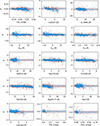 |
Fig. A.1. Residuals across the MILES stellar library. Blue symbols correspond to the difference between the FASTAR line-strengths predictions and the actual measurements over the MILES empirical spectra. For comparison, orange symbols indicate the predictions from the MILES interpolator. Dashed lines correspond to the mean of the distribution and shaded areas to the 1σ scatter. |
As already showcased in Fig. 4, both interpolation schemes perform at a similar level, with FASTAR yielding generally a slightly smaller scatter. Some features such as the Mgb 5177 or the Ca 4227 show a small but noticeable non-linearity in the residual distribution due to differences between the empirical MILES and theoretical BOSZ predictions used for training. Yet, in general, the agreement between both interpolators is remarkable, even in features such as the Balmer lines that traditionally pose problems when comparing theoretical and empirical predictions due to non-LTE effects (Knowles et al. 2023). In FASTAR, predictions tend to be close to the empirical expectations because the training has been intentionally biased toward MILES through the augmentation process.
It is also worth emphasizing that the FASTAR interpolation has been trained to match both theoretical and empirical libraries, while Fig. A.1 only reflects its performance compared to the empirical stars of MILES. In other words, FASTAR is able to incorporate information about the theoretical BOSZ library while predicting empirical data at the same level as the MILES interpolation. Moreover, the training loss is evaluated based on the PCA components, not, for example, on the line-strength behavior. Then, it would be straightforward to optimize these predictions by explicitly training to also match line-strength predictions, which will be explored in upcoming releases.
Appendix B: TiO2 behavior
The predicted TiO2 values for FASTAR SSP models present a significant systematic deviation with respect to the MILES SSP models, as shown in Fig. 6. Following Fig. B.1, we interpret this as a consequence of the different behavior of the index with metallicity for stars cooler than log Teff ∼ 3.6 in the MILES and BOSZ libraries.
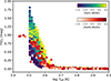 |
Fig. B.1. Empirical versus theoretical TiO2 behavior. MILES stars (red symbols) do not exhibit a significant trend with metallicity at low effective temperatures, contrary to the BOSZ library. This explains the differences between FASTAR and MILES in the TiO2 values predicted for SSP models 6. |
It is evident from this figure that, in general, MILES and BOSZ predictions are similar, but MILES stars do not present a significant dependence on metallicity, while stars in the theoretical BOSZ do. However, as noted in the main text, the modeling of broad molecular features can be particularly problematic and prone to systematics whose effects can propagate to both empirical and theoretical stellar libraries. Moreover, the range of metallicities covered by MILES for cool stars is also significantly narrower than that probed by BOSZ.
Appendix C: SSP predictions for line-strength indices
In the main text we showcase the behavior of FASTAR and MILES SSP predictions for three indices, HβO, Mgb, and TiO2. While that comparison shows an overall good agreement between both sets of models, as well as some differences, Fig. 6 does not fully characterize the behavior of FASTAR SSP models.
In Fig. C.1 we include a larger set of indices, contrasting the FASTAR (in blue) and MILES predictions (in orange) for varying age, metallicity and IMF slope (under a bimodal parameterization in this case). Despite the differences in ingredients and assumptions, Fig. C.1 shows a remarkable agreement between FASTAR and MILES. From different Balmer lines to features sensitive to metallicity and IMF, the trends and even absolute values predicted by both sets of models are notably similar. Although model systematics are, in general, a limiting factor of SSP modelling, the similarities between FASTAR and MILES shown in Fig. C.1 clearly speaks in favor of the consistency and robustness of evolutionary stellar population models.
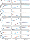 |
Fig. C.1. FASTAR versus MILES SSP predictions. Each row shows the dependence of a specific line-strength index with age (left), metallicity (middle) and IMF slope (right, under a bimodal parameterization) for FASTAR (in blue) and MILES (orange) SSP models. In each column, the value of the assumed age, metallicity and IMF slope is indicated in the first row (corresponding to the CaHK feature). Equivalent widths are calculated at the 2.51 Å nominal resolution of both sets of models. |
As expected, the largest systematic differences between FASTAR and MILES happen at the extremes of the metallicity range. For example, for the CaHK feature (using the Serven et al. 2005 definition), the agreement increases for those metallicities around the solar value where the importance of MILES empirical templates is maximal. For the case of the TiO1 and TiO2 features, the differences in the metallicity dependence between MILES and BOSZ (see Appendix B) become evident at the SSP level.
All Tables
All Figures
|
Fig. 1. IMF functional forms. FASTAR comes with the six pre-defined IMF parameterizations shown here. All of their parameters can be changed to synthesize new models with variable IMFs. In addition, models for any arbitrary IMF defined by the user can also be calculated. |
| In the text | |
|
Fig. 2. Performance of the FASTAR interpolator across the log g-Teff-[Fe/H] parameter space. Each star in the MILES and BOSZ libraries is color coded by the reconstruction error, defined as the standard deviation of the residuals between the real spectrum and the predicted one. The top panel shows the log g-Teff, while the bottom one shows log g-[Fe/H]. The average error is on the order of ∼3%, only becoming closer to ∼10% for the coolest stars in the sample. There is no significant trend with metallicity. |
| In the text | |
|
Fig. 3. Comparison of residuals. Blue and orange lines represent the distribution of residuals for the FASTAR and MILES interpolators when predicting the stellar spectra of the MILES library. The behavior of both interpolation schemes is similar, as shown by the vertical dashed lines marking the 20th and 80th percentiles. However, the 2nd and 98th percentile vertical lines indicate that extreme errors are less common in FASTAR. For comparison, the gray histogram shows the error associated to the PCA compression. |
| In the text | |
|
Fig. 4. Line-strength and color comparison. Observed (horizontal axes) line-strength and colors are compared to the predicted values (vertical axes) using the FASTAR (blue filled circles) and MILES (orange squares) interpolators. From left to right, we show the behavior of the metallicity-sensitive [MgFe]’ (Thomas et al. 2003), the age-sensitive HβO (Cervantes & Vazdekis 2009), and the IMF-sensitive TiO2 (Faber et al. 1985; Trager et al. 1998). The panel on the right shows the comparison of the (g − r) color. The interpolation in FASTAR tends to outperform that of MILES, with systematically smaller residuals as indicated on the bottom right corner of each panel. |
| In the text | |
|
Fig. 5. FASTAR spectroscopic and photometric predictions. Blue lines show to the FASTAR SSP models for a 10 Gyr old, solar metallicity population. In light blue, the FASTAR photometric model is based on the BOSZ theoretical stellar library and can be convolved with any set of photometric filters (exemplified by the different transmission functions in grey) to generate photometric predictions. In addition, the spectroscopic side of FASTAR (dark blue line) combines the MILES (empirical) and BOSZ stellar libraries to generate models oriented toward detailed stellar population analyses. |
| In the text | |
|
Fig. 6. Line-strength comparison. Blue and orange lines indicate, respectively, the FASTAR and MILES predictions for different line-strength indices at a 2.51 Å resolution. Left panel: Equivalent width of the HβO line is shown as a function of age for a population of solar metallicity and a Milky Way-like IMF. For old ages, FASTAR predictions tend to be lower than those of MILES. Middle panel: dependence of the Mgb feature on metallicity for a 10 Gyr population with a Milky Way-like IMF. Right panel: Behavior of the TiO2 molecular band for different IMF slope values (single power law) is shown for 10 Gyr and solar metallicity population. |
| In the text | |
|
Fig. 7. Color predictions. From left to right, each panel shows the color sensitivity of the photometric and spectroscopic FASTAR models (dashed and solid blue lines, respectively), as well as the MILES predictions (in orange) for comparison. The differences between the three models are due to the use of theoretical versus empirical stellar libraries and the choice of bolometric corrections (between FASTAR and MILES). The assumed ages, metallicities and IMF slopes are the same as in Fig. 6. |
| In the text | |
|
Fig. 8. Mass-to-light ratio and magnitude trends. Solid lines and left vertical axes represent the change in stellar M/L as a function of age (left), metallicity (middle), and IMF slope (right). When not varied, the age is fixed to 10 Gyr, the metallicity to solar, and the IMF to the Milky Way value. Similarly, dashed lines and right axes correspond to the expected absolute magnitude of the population. FASTAR predictions for the SDSS g band are shown in green while the expectation for the near-infrared JWST/NIRCam F090W filter are shown in red. |
| In the text | |
|
Fig. 9. Optimal age sampling. Top: Relative age sensitivity of FASTAR SSP models as a function of age. The normalized age derivative of the FASTAR models becomes smaller for older ages, reflecting the fact that age variations have a progressively weaker effect on the integrated spectrum of a galaxy with increasing age. The peak contribution of the AGB (and RGB) phases appears as a sudden change in the derivative at an age of ∼1.5 Gyr. Bottom: Age sampling of the MILES models is shown in red, following their BaSTI isochrone grid. In blue, the optimized FASTAR sampling enforces a constant flux variation across all age bins. |
| In the text | |
|
Fig. 10. Uncertainty of SSP model predictions. The upper panel shows the SSP model predicted by FASTAR for a population of 10 Gyr and solar metallicity while the bottom panel shows the associated errors. In purple, we present the uncertainty in the SSP model assuming a typical error Δlog g = 0.2 dex in the determination of the surface gravity of the stars. In red and yellow we represent the error corresponding to the metallicity (Δ[Fe/H] = 0.1 dex) and effective temperature (ΔTeff = 0.005 dex), respectively. In grey, we show the expected total uncertainty in the SSP model. |
| In the text | |
|
Fig. 11. Stellar predictions across different spectral types. Dark and light lines represent predictions using both the MILES and BOSZ stellar libraries, and using only BOSZ, respectively. Each color corresponds to a different stellar type, as indicated by the labels. |
| In the text | |
|
Fig. 12. Line-strength HβO versus [MgFe]’ index-index diagram for Milky Way globular clusters. Filled symbols correspond to the globular cluster sample of Usher et al. (2017), color coded by their [Fe/H] metallicity. The FASTAR model grid prediction is shown in the background in grey. Labels indicate ages and metallicities across the grid. The equivalent width for data and models is measured at the FASTAR 2.51 Å spectral resolution. FASTAR model predictions reproduce the observed data without systematic offsets, suggesting that the well-known zero-point problem of evolutionary stellar population models can be at least minimized with state-of-the art isochrones. |
| In the text | |
|
Fig. 13. Globular clusters in the Fornax Cluster. Filled circles correspond to the (g − z) versus [MgFe]’ values measured in the Fahrion et al. (2020) sample of globular clusters in the Fornax galaxy cluster, with the color coding representing their total metallicity. The background model grid shows the FASTAR predictions for different ages and metallicities, with the (g − z) and [MgFe]’ values, coming from the FASTAR photometric and spectroscopic sets of predictions, respectively. |
| In the text | |
|
Fig. 14. Globular clusters in M 31. The (u − g) versus (g − r) colors of globular clusters in M 31 are shown, color coded by their iron metallicity, as reported in Caldwell et al. (2011). To minimize the effect of dust, the sample has been reduced to those globular clusters with E(B − V) < 0.15. The gray background grid shows the FASTAR photometric predictions for different ages and metallicities, for a fixed Milky Way-like IMF. |
| In the text | |
|
Fig. 15. Ages and metallicities of quiescent early-type galaxies. Filled symbols correspond to the HβO and [MgFe]’ line-strength measured over the stacked SDSS spectra of La Barbera et al. (2013), with the color code given by the mean stellar velocity dispersion of each stack. The background model grid shows the FASTAR predictions for those two indices for a Milky Way IMF (solid lines). For reference, the grid for a bottom-heavy IMF (single power law with α = 3) is also shown with dashed lines. As expected, the prediction from the FASTAR models is that quiescent early-type galaxies become increasingly more metal-rich and older when increasing velocity dispersion. Models and data have been convolved to the resolution of the highest σ stack. |
| In the text | |
|
Fig. 16. Fits to SDSS stacked spectra. The MILES (in orange) and FASTAR (in blue) best-fitting models are shown compared to two SDSS stacked spectra (in black). The top and bottom panels correspond to stacks of low-σ (110 km s−1) and high-σ (280 km s−1) early-type galaxies, respectively. MILES and FASTAR best-fitting models are very similar as demonstrated by the residual distribution also displayed in each panel. No polynomial correction was applied to the continuum. |
| In the text | |
|
Fig. 17. Age-velocity dispersion relation. Blue and orange symbols correspond to the best-fitting ages of the SDSS stacked spectra using pPXF and the FASTAR and MILES SSP models, respectively, while filled and empty symbols indicate mass- and luminosity-weighted values. FASTAR and MILES models are able to retrieve the expected age-σ relation, with FASTAR-based ages generally being younger than those measured with MILES. |
| In the text | |
|
Fig. 18. Metallicity-velocity dispersion relation. The symbols and colors are the same as in Fig. 17, but in this case they represent the best-fitting metallicity values. The expected relation with velocity dispersion is well recovered with both sets of models although with systematic differences as FASTAR tends to result in lower metallicities and less differences between mass-weighted and luminosity-weighted values than MILES. |
| In the text | |
|
Fig. A.1. Residuals across the MILES stellar library. Blue symbols correspond to the difference between the FASTAR line-strengths predictions and the actual measurements over the MILES empirical spectra. For comparison, orange symbols indicate the predictions from the MILES interpolator. Dashed lines correspond to the mean of the distribution and shaded areas to the 1σ scatter. |
| In the text | |
|
Fig. B.1. Empirical versus theoretical TiO2 behavior. MILES stars (red symbols) do not exhibit a significant trend with metallicity at low effective temperatures, contrary to the BOSZ library. This explains the differences between FASTAR and MILES in the TiO2 values predicted for SSP models 6. |
| In the text | |
|
Fig. C.1. FASTAR versus MILES SSP predictions. Each row shows the dependence of a specific line-strength index with age (left), metallicity (middle) and IMF slope (right, under a bimodal parameterization) for FASTAR (in blue) and MILES (orange) SSP models. In each column, the value of the assumed age, metallicity and IMF slope is indicated in the first row (corresponding to the CaHK feature). Equivalent widths are calculated at the 2.51 Å nominal resolution of both sets of models. |
| In the text | |
Current usage metrics show cumulative count of Article Views (full-text article views including HTML views, PDF and ePub downloads, according to the available data) and Abstracts Views on Vision4Press platform.
Data correspond to usage on the plateform after 2015. The current usage metrics is available 48-96 hours after online publication and is updated daily on week days.
Initial download of the metrics may take a while.