| Issue |
A&A
Volume 691, November 2024
|
|
|---|---|---|
| Article Number | L10 | |
| Number of page(s) | 5 | |
| Section | Letters to the Editor | |
| DOI | https://doi.org/10.1051/0004-6361/202451604 | |
| Published online | 08 November 2024 | |
Letter to the Editor
Counting stars from the integrated spectra of galaxies
1
Instituto de Astrofísica de Canarias, c/ Vía Láctea s/n, E38205 La Laguna, Tenerife, Spain
2
Departamento de Astrofísica, Universidad de La Laguna, E-38205 La Laguna, Tenerife, Spain
⋆ Corresponding authors; This email address is being protected from spambots. You need JavaScript enabled to view it.
; This email address is being protected from spambots. You need JavaScript enabled to view it.
Received:
22
July
2024
Accepted:
11
October
2024
Abstract
Over the last few decades, evolutionary population synthesis models have powered an unmatched leap forward in our understanding of galaxies. From dating the age of the first galaxies in the Universe to providing detailed measurements of the chemical composition of nearby galaxies, the success of this approach built upon simple stellar population (SSP) spectro-photometric models is unquestionable. However, the internal constraints inherent to the construction of SSP models can hinder our ability to analyze the integrated spectra of galaxies in situations where the SSP assumption does not sufficiently hold. Thus, here we revisit the possibilities of fitting galaxy spectra as a linear combination of stellar templates without assuming any a priori knowledge on stellar evolution. We showcase the sensitivity of this alternative approach to changes in the stellar population properties, in particular the direct connection to variations in the stellar initial mass function, as well as its advantages when dealing with noncanonical integrated populations and semi-resolved observations. Furthermore, our analysis demonstrates that the absorption spectra of galaxies can be used to independently constrain stellar evolution theory beyond the limited conditions of the solar neighborhood.
Key words: galaxies: evolution / galaxies: formation / galaxies: stellar content
© The Authors 2024
 Open Access article, published by EDP Sciences, under the terms of the Creative Commons Attribution License (https://creativecommons.org/licenses/by/4.0), which permits unrestricted use, distribution, and reproduction in any medium, provided the original work is properly cited.
This article is published in open access under the Subscribe to Open model. This email address is being protected from spambots. You need JavaScript enabled to view it. to support open access publication.
1. Introduction
The stellar absorption spectrum of a galaxy is the linear combination of the flux emitted by its individual stars. Although this statement may sound obvious, it has immediate implications since it enables us to anchor and interpret observations of distant galaxies based on the well-calibrated properties and thoroughly tested physics of nearby stars. Arguably, the most direct way to analyze the integrated spectrum of a galaxy is to compare it to a set of stellar spectra, also known as empirical modeling. Finding a linear combination of stars that can reproduce an observed spectrum was recognized early on as a viable way forward (Öhman 1934; Whipple 1935), and since then, variations of this method (including the use of star cluster spectra as templates) led to substantial advances in our description of the stellar population content of galaxies (e.g., Spinrad & Taylor 1971; Faber 1972; Pickles 1985; Bica & Alloin 1986; Bica 1988; Schmidt et al. 1991). The main difficulty that these initial attempts encountered was, however, the uniqueness of the recovered solution (e.g., Pelat 1998) and thus the consistency of the inferred properties across different wavelength ranges (e.g., Eftekhari et al. 2022).
Instead of freely combining individual stellar spectra, knowledge on stellar evolution theory can also be assumed in order to model the spectrum of a galaxy. This approach, pioneered by the seminal work of Beatrice Tinsley (Tinsley 1968, 1972; Tinsley & Gunn 1976; Tinsley 1980), sets fixed but physically motivated internal constraints on both the properties (through theoretical isochrones; e.g., Bertelli et al. 1994; Pietrinferni et al. 2004; Choi et al. 2016) and the relative number of stars, that is, the initial mass function (IMF; e.g., Kroupa 2002; Chabrier 2003), that are required to generate the model spectrum of a stellar population. This so-called evolutionary population synthesis technique predicts the absorption spectrum of a simple stellar population (SSP) given its age and chemical composition1. Over the last few decades, SSP model predictions have reached an exquisite level of refinement (e.g., Leitherer et al. 1999; Bruzual & Charlot 2003; Thomas et al. 2003; Schiavon 2007; Vazdekis et al. 2010; Conroy & van Dokkum 2012), which in turn has revolutionized our view of galaxy formation and evolution (e.g., Worthey et al. 1992; Vazdekis et al. 1997; Gallazzi et al. 2005; Thomas et al. 2005; Kuntschner et al. 2006; van Dokkum & Conroy 2010; La Barbera et al. 2013; McDermid et al. 2015).
In parallel to the development of SSP models, the mathematical tools for analyzing the integrated spectra of galaxies have also experienced a significant leap forward. In particular, spectral fitting algorithms able to model an observed spectrum as a linear combinations of SSPs are now widely available (e.g., Cappellari & Emsellem 2004; Cid Fernandes et al. 2005; Ocvirk et al. 2006; Tojeiro et al. 2007; Koleva et al. 2009; Sánchez et al. 2016; Carnall et al. 2019; Johnson et al. 2021), allowing the analysis of populations with complex and extended star formation histories as well.
The success of evolutionary population synthesis models is, therefore, irrefutable. However, the hard-coded assumptions inherent to this approach are not free from biases and potential flaws. For example, fundamental ingredients in the calculation of theoretical isochrones (opacities, mass losses, mixing length, convection, etc.; see, e.g., Maraston 2005; Conroy et al. 2009) are generally weakly constrained or approximated. The decades-long debate about the morphology of the horizontal branch is a paradigmatic example of the current limitations of stellar evolution theory (e.g., Sandage & Wildey 1967; Lee et al. 1994; Dotter et al. 2007). In addition, noncanonical evolutionary pathways such as the contribution of binary stars or extreme mass-loss phases can also have an important contribution to the observed spectrum yet remain poorly incorporated into SSP model predictions (e.g., Renzini & Fusi Pecci 1988; Greggio & Renzini 1990; Eldridge et al. 2017).
Two recent developments have further highlighted some of the limitations of evolutionary population synthesis models. First, the apparent non-universality of the IMF (e.g., Ferreras et al. 2013; Spiniello et al. 2014; Martín-Navarro et al. 2015; Parikh et al. 2018) casts doubts on the flexibility of SSP models to account for complex IMF variations (Conroy et al. 2017), particularly when dealing with young stellar populations (Martín-Navarro et al. 2024). Finally, a new generation of spectroscopic facilities, such as the Local Volume Mapper (Drory et al. 2024) and most importantly the European Extremely Large Telescope (Gilmozzi & Spyromilio 2007) and the US Extremely Large Telescope Program (Wolff et al. 2019), will observe the nearby Universe in a semi-resolved manner, where the basic assumption behind SSP models of a fully sampled IMF no longer holds.
In this Letter we revisit the possibilities of a more agnostic approach to stellar population inference, fitting integrated absorption spectra of galaxies as a linear combination of stellar spectra. Equipped with state-of-the-art spectral fitting algorithms and stellar libraries, we demonstrate some of the unique advantages of this approach as well as its potential limitations. The outline of this work is as follows: In Sect. 2 we describe the fitting scheme and in Sect. 3 present a series of consistency tests. In Sect. 4 we discuss our results and point toward some interesting prospects.
2. Fitting scheme
We based our analysis on the penalized pixel-fitting (pPXF) algorithm (Cappellari & Emsellem 2004). In short, pPXF was designed to fit the integrated spectra of galaxies as a linear combination of SSP model predictions. Thus, the basic output of pPXF is a weights matrix defining the relative contribution of each SSP model to the observed spectrum. Moreover, as described in detail in Cappellari (2017), pPXF is able to retrieve robust stellar population measurements by regularizing the recovered weights in up to three dimensions. Then, pPXF is usually paired with a set of SSP models that cover a range of ages, metallicities, and [α/Fe] to derive star formation histories and chemical enrichment patterns.
For individual stars, a library of stellar spectra is also characterized by three main parameters, namely log g, Teff, and [Fe/H]. With this idea in mind, we paired pPXF with the MILES stellar library presented in Sánchez-Blázquez et al. (2006). However, MILES is an empirical stellar library and thus stars are not homogeneously distributed across the whole log g–Teff–[Fe/H] parameter space. Therefore, to maximize the capabilities of pPXF, we used the roughly 1000 stars from the MILES library and the interpolation scheme described in Vazdekis et al. (2003) and updated in Vazdekis et al. (2010) to generate a regular grid of stellar spectra. It is worth highlighting that, according to stellar evolution theory, stars with different masses (and thus different log g and Teff) have different luminosities. However, we intentionally did not want to include any additional information during the fitting process. Hence, we neglected the expected differences in luminosity, and the flux of each stellar template was normalized to the same value, regardless of its mass. The importance of this decision will become obvious in the next section.
3. Results
3.1. Fitting SSP models
An immediate way to assess the reliability of our approach is to fit, using individual stars, SSP model predictions constructed with the very same stellar spectra. In Fig. 1 we show the flux weights distribution recovered when fitting a MILES model of 10 Gyr and solar metallicity with the MILES stellar library. Overplotted on the weights distribution, we also show a Pietrinferni et al. (2004, scaled solar) theoretical isochrone for a 10 Gyr, solar metallicity population that was used to generate the MILES SSP model.
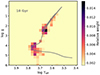 |
Fig. 1. Best-fitting solution for an SSP model. Each pixel in the image corresponds to the relative flux contribution of stars with different log g and Teff that best reproduce a MILES SSP model of 10 Gyr and solar metallicity. The gray line indicates a theoretical isochrone with the same age and metallicity used to build the MILES SSP model. |
It is clear from Fig. 1 that the flux weights recovered by pPXF are not randomly distributed but closely follow the isochrone track. This result is particularly noteworthy because no stellar evolution knowledge has been implemented in the code and the inversion problem is highly degenerate (Schmidt et al. 1991; Eftekhari et al. 2022), even more than in the case of SSP models (e.g., Worthey 1994), since for a single SSP model pPXF has to explore a parameter space as large as would be required to measure the whole star formation history of a galaxy. Yet, pPXF fed with the MILES stellar library is able to retrieve a physically meaningful solution. We note that the value of the recovered weights along the isochrone depends on two main factors: the intrinsic luminosity of stars with that particular mass and the number of them (i.e., the IMF). Therefore, the flux weights are dominated by the contribution of luminous giant stars (the prominence of the red clump is particularly evident) and by the relatively bright and heavily populated main sequence turnoff.
We expanded this series of consistency tests and show in Fig. 2 the result of fitting SSP models with different ages, IMF slopes, and metallicities. In the left panel, the weights distribution of a young 5 Gyr population with solar metallicity is shown. While there is a small yet noticeable difference in the position of the main sequence turnoff, the most evident change with respect to Fig. 1 is the relatively large weights given to these turnoff stars when fitting the 5 Gyr population, which simply reflects the presence of hotter and more massive (i.e., more luminous) stars. Interestingly, changes in the IMF slope are also propagated to the recovered weights distribution, as shown in the middle panel of Fig. 2. In this case, we again fit an SSP model of 10 Gyr and solar metallicity but with a bottom-heavy (i.e., dwarf-rich) IMF. There are two key differences between the results shown in this middle panel and in Fig. 1. First, the relative dwarfs-to-giants weight is higher in this case, as expected from the change in the IMF slope. Second, pPXF tends to give weights to stars with even lower stellar masses (i.e., log g ≳ 4.5 and log Teff ≲ 3.6). Thus, in an idealized scenario, the proposed setup can also be sensitive, in a nonparametric way, to changes in the IMF. This, however, would require a physically motivated normalization for each stellar template. Finally, the right panel of Fig. 2 shows the recovered metallicity distribution for two SSP models: in red for a metal rich population ([M/H] = 0.26) and in blue for a metal-poor one ([M/H] = –0.66). Again, changes in the metallicity of the underlying stellar population are systematically recovered.
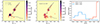 |
Fig. 2. Sensitivity to changes in the stellar population properties. Left: Weights distribution retrieved after fitting the MILES SSP model prediction of a population with solar metallicity and an age of 5 Gyr, with two isochrones of 5 and 10 Gyr overplotted for comparison. Middle: Similar weights distribution but for an old (10 Gyr) solar metallicity population with a relative excess of low-mass stars (i.e., a bottom-heavy IMF). In this case, the isochrone corresponds to a 10 Gyr population. Right: Recovered metallicity weights after fitting two MILES SSP models, in red and blue for a metal-rich and a metal-poor population, respectively. |
3.2. Noncanonical stellar populations
An obvious advantage of our fitting scheme is the possibility of dealing with noncanonical stellar populations. To exemplify this, we briefly present the results from Salvador-Rusiñol et al. (2022), who discuss two scenarios to explain the line-strength ratios of UV indices in the spectrum of the massive galaxy NGC 1277. On the one hand, the measured line-strength indices can be explained by the presence of some residual star formation and thus young, massive stars on top of an underlying old stellar population. On the other, the observed line-strength ratios can also be interpreted as a combination of the same old stellar population plus the contribution of an additional similarly old population with a peculiarly extreme horizontal branch.
In particular, Salvador-Rusiñol et al. (2022) invoke a combination of a ∼13 Gyr population plus a 0.5% contribution of ∼0.1 Gyr for the first scenario, or the same old population combined with 40% of a second SSP characterized by an extreme horizontal branch. Using these values, we generated two synthetic spectra corresponding to each hypothesis and analyzed them using our fitting approach. The result of this test is shown in Fig. 3.
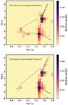 |
Fig. 3. Young populations vs. extreme horizontal branch stars. Top: Weights distribution measured for a synthetic spectrum combining a dominant old population (13 Gyr) and a 0.5% contribution from an SSP with ∼0.1 Gyr. Solid and dashed gray lines indicate the isochrones of the old and young populations, respectively. The recovered weights follow the tracks defined by both isochrones. Bottom: Similar weights distribution but for the combination of the same old population plus 40% of an SSP with an extreme horizontal branch. Again, solid and dashed gray lines indicate the theoretical isochrones used to build the models. |
The top panel of Fig. 3 shows the recovered weights for the case of a residual young population on top of the dominant old component. Overplotted on these weights are the isochrones assumed to generate the two populations. In addition to the main 13 Gyr population that dominates the weights distribution, stars around the main sequence turnoff of the secondary young population are also clearly recovered by the fitting scheme. In the bottom panel, corresponding to the second scenario with an extreme horizontal branch population, the measured weights distribution is clearly different, lacking the characteristic turnoff stars shown in the upper panel. From the results of this test, it is evident the advantage of this approach, fitting in a nonparametric way the absorption spectra of stellar populations that depart from the internal assumptions of SSP models.
3.3. Fitting observed galaxy spectra
The above results are idealized scenarios to demonstrate some of the potential applications of a physics-free fit to the integrated spectra of galaxies. To test the feasibility of this approach when dealing with real data, we analyzed the Sloan Digital Sky Survey (SDSS; Adelman-McCarthy et al. 2008) stacked spectra from La Barbera et al. (2013). In short, they consist of 16 high signal-to-noise stacked spectra of nearby early-type galaxies (ETGs) that cover a range of stellar velocity dispersions. These spectra have been previously studied in detail (see, e.g., Ferreras et al. 2013; La Barbera et al. 2013; Rosani et al. 2018; Pernet et al. 2024), and thus we can use them to assess the robustness of our approach.
The top panel of Fig. 4 shows the measured iron metallicity of the SDSS stacked spectra based on the combination of MILES stars as a function of the stellar velocity dispersion, σ. As anticipated by the right panel in Fig. 2, the proposed approach is sensitive to changes in the metallicity content of the absorption spectra, recovering in this case the well-known metallicity-σ relation. It is worth noting that our measurements are based on the iron metallicity ([Fe/H]) of the individual MILES stars. In this regard, the recovered trend coincides with the line-strength analysis of La Barbera et al. (2013), who found a variation in [Fe/H] from −0.17 to −0.04 between the low-σ and high-σ SDSS stacked spectra, once corrected for the measured [Mg/Fe] abundance ratio.
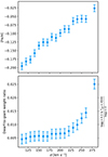 |
Fig. 4. Fits to SDSS data. Top: Measured iron metallicity values as a function of stellar velocity dispersion for the SDSS stacked spectra. We recover the well-known relation between the metallicity of galaxies and their velocity dispersions based on the linear combination of MILES stars. Note that metallicity refers here to [Fe/H] as it is based on the metallicity of these individual stars. Bottom: Ratio between the weight given to low-mass and high-mass stars by our fitting approach. This weight ratio is a proxy for variations in the IMF and suggests a relative excess of low-mass stars in the most massive ETGs. |
Inspired by the comparison between Fig. 1 and the middle panel of Fig. 2, we also assessed the possibility of measuring the effect of a variable IMF. For the SDSS sample, detailed line-strength (SSP-based) measurements have revealed a systematic variation in the IMF slope, with galaxies with higher σ exhibiting a higher fraction of low-mass stars (Ferreras et al. 2013; La Barbera et al. 2013; Martín-Navarro et al. 2019; den Brok et al. 2024). Our approach is directly connected to the IMF of the analyzed stellar population since the measured weights are effectively mapping the number of stars as a function of their mass, modulated by their luminosity. Moreover, the proposed approach probes the IMF in a nonparametric way, in principle allowing for any kind of underlying change in the IMF.
Capitalizing on this key feature, the bottom panel of Fig. 4 shows the ratio between the flux weight given to low-mass M-dwarf stars (log g > 4.5 and Teff < 4500) and the flux weight given to giant stars (log g < 3). Because of the rather old ages of the sample, this metric approximates the dwarf-to-giant ratio traditionally measured in ETGs to quantify changes in the IMF slope. In the bottom panel of Fig. 4, it is clear that our approach also points toward a systematic change in the IMF: the weights given to low-mass stars in order to fit the observed spectra become progressively more important for more massive galaxies. This finding is in remarkable agreement with the expectations based on alternative stellar population analyses.
4. Discussion and prospects
Interpreting the integrated spectra of galaxies with as few model assumptions as possible is the ultimate goal of any stellar population analysis. In this context, the development of evolutionary population synthesis models has been a necessary and extremely successful stepping stone. Yet, we have demonstrated here that it is now possible to further distill the modeling process, reducing it to its most basic components: the spectra of individual stars. The fact that the measured weights shown in, for example, Fig. 1 are not sparsely distributed but follow the track of theoretical isochrones is a striking result. It shows that there is physically meaningful information about stellar evolution theory and about the number distribution of stars encoded in the integrated spectra of galaxies.
There are two immediate applications for these findings. First, it is possible to use integrated spectra, decomposed into the flux of individual stars, to constrain the physical ingredients that go into the calculation process of evolutionary population synthesis models, and more generally, to improve our knowledge of stellar evolution theory. Second, it provides more direct access to the IMF of unresolved stellar populations. In particular, the rigidity of SSP models has so far severely hampered our ability to compare dynamical and stellar population-based IMF measurements (e.g., Oldham & Auger 2018; Poci et al. 2021). The model-independent approach outlined here (see also Dries et al. 2016) presents a unique opportunity to model in a self-consistent way the properties and dynamics of individual stars beyond the Milky Way (e.g., van de Ven et al. 2008; Zhu et al. 2018; Vasiliev & Valluri 2020).
It is also worth mentioning that, although the above results are promising, there are several aspects of the fitting scheme that can be significantly improved. For example, while the way that the regularization of the solution is implemented in pPXF is ideally suited to work with SSP models when smooth changes are expected in the star formation history and chemical enrichment (and thus the recovered weights), it does not necessarily apply to the weight distribution of individual stars since the expected smoothness of the solution is high along the isochrone but low in the orthogonal direction. Moreover, metallicity, luminosity, log g, and Teff are not fully independent quantities and thus the degree of freedom of the inversion problem tackled in this work, and consequently the associated uncertainties, has been artificially amplified. Finally, translating weights into physical quantities such as ages or chemical compositions would require an additional modeling layer, as in resolved stellar populations analyses (e.g., Gallart et al. 2005). Ultimately, the proposed approach will require dedicated tools and templates to fully maximize its potential applications.
With all this in mind, could a physics-free approach replace the use of SSP models? In the foreseeable future, SSP model predictions will likely remain a fundamental tool for stellar population analyses. In many situations, the complexity and intrinsic degeneracies of the inversion problem, amplified by the noisy nature of real data, can only be partially mitigated through the internal constraints of evolutionary population synthesis models. Ultimately, our ability to retrieve information about the stellar population properties of galaxies depends on the (limited) amount of information encoded in their absorption spectra (e.g., Ferreras et al. 2023).
However, as demonstrated here, there are several advantages to fitting the absorption spectra of galaxies using stellar spectra, and the two approaches can actually complement each other. Moreover, there are some important questions that can only be tackled outside of the rigid limits of SSP models. With larger and better stellar libraries (García Pérez et al. 2021; Yan et al. 2019; Knowles et al. 2021), the advent of a new generation of observational facilities, and the current explosion of computational capabilities, it is possible to rethink our approach to stellar population models, aspiring to gain access to new information about the star formation processes in galaxies.
Nowadays, the term SSP usually refers to the actual spectral model of a stellar population.
Acknowledgments
We would like to thank the comments and suggestions from the referee which help improving the manuscript. IMN would like to thank Bron Reichardt-hu, Dimitri Gadotti, Sebastián Sánchez, Glenn van de Ven and the TRACES group for the discussions that sparked some of the ideas motivating this work. We acknowledge support from grant PID2022-140869NB-I00 from the Spanish Ministry of Science and Innovation.
References
- Adelman-McCarthy, J. K., Agüeros, M. A., Allam, S. S., et al. 2008, ApJS, 175, 297 [NASA ADS] [CrossRef] [Google Scholar]
- Bertelli, G., Bressan, A., Chiosi, C., Fagotto, F., & Nasi, E. 1994, A&AS, 106, 275 [NASA ADS] [Google Scholar]
- Bica, E. 1988, A&A, 195, 76 [NASA ADS] [Google Scholar]
- Bica, E., & Alloin, D. 1986, A&A, 162, 21 [NASA ADS] [Google Scholar]
- Bruzual, G., & Charlot, S. 2003, MNRAS, 344, 1000 [NASA ADS] [CrossRef] [Google Scholar]
- Cappellari, M. 2017, MNRAS, 466, 798 [Google Scholar]
- Cappellari, M., & Emsellem, E. 2004, PASP, 116, 138 [Google Scholar]
- Carnall, A. C., Leja, J., Johnson, B. D., et al. 2019, ApJ, 873, 44 [Google Scholar]
- Chabrier, G. 2003, PASP, 115, 763 [Google Scholar]
- Choi, J., Dotter, A., Conroy, C., et al. 2016, ApJ, 823, 102 [Google Scholar]
- Cid Fernandes, R., Mateus, A., Sodré, L., Stasińska, G., & Gomes, J. M. 2005, MNRAS, 358, 363 [Google Scholar]
- Conroy, C., & van Dokkum, P. G. 2012, ApJ, 760, 71 [Google Scholar]
- Conroy, C., Gunn, J. E., & White, M. 2009, ApJ, 699, 486 [Google Scholar]
- Conroy, C., van Dokkum, P. G., & Villaume, A. 2017, ApJ, 837, 166 [NASA ADS] [CrossRef] [Google Scholar]
- den Brok, M., Krajnović, D., Emsellem, E., et al. 2024, MNRAS, 530, 3278 [NASA ADS] [CrossRef] [Google Scholar]
- Dotter, A., Chaboyer, B., Jevremović, D., et al. 2007, AJ, 134, 376 [NASA ADS] [CrossRef] [Google Scholar]
- Dries, M., Trager, S. C., & Koopmans, L. V. E. 2016, MNRAS, 463, 886 [CrossRef] [Google Scholar]
- Drory, N., Blanc, G. A., Kreckel, K., et al. 2024, AJ, 168, 198 [NASA ADS] [CrossRef] [Google Scholar]
- Eftekhari, E., La Barbera, F., Vazdekis, A., Allende Prieto, C., & Knowles, A. T. 2022, MNRAS, 512, 378 [NASA ADS] [CrossRef] [Google Scholar]
- Eldridge, J. J., Stanway, E. R., Xiao, L., et al. 2017, PASA, 34, e058 [Google Scholar]
- Faber, S. M. 1972, A&A, 20, 361 [NASA ADS] [Google Scholar]
- Ferreras, I., La Barbera, F., de la Rosa, I. G., et al. 2013, MNRAS, 429, L15 [NASA ADS] [CrossRef] [Google Scholar]
- Ferreras, I., Lahav, O., Somerville, R. S., & Silk, J. 2023, RAS Techn. Instrum., 2, 78 [CrossRef] [Google Scholar]
- Gallart, C., Zoccali, M., & Aparicio, A. 2005, ARA&A, 43, 387 [Google Scholar]
- Gallazzi, A., Charlot, S., Brinchmann, J., White, S. D. M., & Tremonti, C. A. 2005, MNRAS, 362, 41 [Google Scholar]
- García Pérez, A. E., Sánchez-Blázquez, P., Vazdekis, A., et al. 2021, MNRAS, 505, 4496 [CrossRef] [Google Scholar]
- Gilmozzi, R., & Spyromilio, J. 2007, The Messenger, 127, 11 [Google Scholar]
- Greggio, L., & Renzini, A. 1990, ApJ, 364, 35 [Google Scholar]
- Johnson, B. D., Leja, J., Conroy, C., & Speagle, J. S. 2021, ApJS, 254, 22 [NASA ADS] [CrossRef] [Google Scholar]
- Knowles, A. T., Sansom, A. E., Allende Prieto, C., & Vazdekis, A. 2021, MNRAS, 504, 2286 [NASA ADS] [CrossRef] [Google Scholar]
- Koleva, M., Prugniel, P., Bouchard, A., & Wu, Y. 2009, A&A, 501, 1269 [CrossRef] [EDP Sciences] [Google Scholar]
- Kroupa, P. 2002, Science, 295, 82 [Google Scholar]
- Kuntschner, H., Emsellem, E., Bacon, R., et al. 2006, MNRAS, 369, 497 [NASA ADS] [CrossRef] [Google Scholar]
- La Barbera, F., Ferreras, I., Vazdekis, A., et al. 2013, MNRAS, 433, 3017 [Google Scholar]
- Lee, Y.-W., Demarque, P., & Zinn, R. 1994, ApJ, 423, 248 [NASA ADS] [CrossRef] [Google Scholar]
- Leitherer, C., Schaerer, D., Goldader, J. D., et al. 1999, ApJS, 123, 3 [Google Scholar]
- Maraston, C. 2005, MNRAS, 362, 799 [NASA ADS] [CrossRef] [Google Scholar]
- Martín-Navarro, I., La Barbera, F., Vazdekis, A., Falcón-Barroso, J., & Ferreras, I. 2015, MNRAS, 447, 1033 [Google Scholar]
- Martín-Navarro, I., Lyubenova, M., van de Ven, G., et al. 2019, A&A, 626, A124 [Google Scholar]
- Martín-Navarro, I., de Lorenzo-Cáceres, A., Gadotti, D. A., et al. 2024, A&A, 684, A110 [NASA ADS] [CrossRef] [EDP Sciences] [Google Scholar]
- McDermid, R. M., Alatalo, K., Blitz, L., et al. 2015, MNRAS, 448, 3484 [Google Scholar]
- Ocvirk, P., Pichon, C., Lançon, A., & Thiébaut, E. 2006, MNRAS, 365, 46 [Google Scholar]
- Öhman, Y. 1934, ApJ, 80, 171 [CrossRef] [Google Scholar]
- Oldham, L., & Auger, M. 2018, MNRAS, 474, 4169 [NASA ADS] [CrossRef] [Google Scholar]
- Parikh, T., Thomas, D., Maraston, C., et al. 2018, MNRAS, 477, 3954 [Google Scholar]
- Pelat, D. 1998, MNRAS, 299, 877 [NASA ADS] [CrossRef] [Google Scholar]
- Pernet, E., Boecker, A., & Martín-Navarro, I. 2024, A&A, 687, L14 [NASA ADS] [CrossRef] [EDP Sciences] [Google Scholar]
- Pickles, A. J. 1985, ApJ, 296, 340 [NASA ADS] [CrossRef] [Google Scholar]
- Pietrinferni, A., Cassisi, S., Salaris, M., & Castelli, F. 2004, ApJ, 612, 168 [Google Scholar]
- Poci, A., McDermid, R. M., Lyubenova, M., et al. 2021, A&A, 647, A145 [NASA ADS] [CrossRef] [EDP Sciences] [Google Scholar]
- Renzini, A., & Fusi Pecci, F. 1988, ARA&A, 26, 199 [NASA ADS] [CrossRef] [Google Scholar]
- Rosani, G., Pasquali, A., La Barbera, F., Ferreras, I., & Vazdekis, A. 2018, MNRAS, 476, 5233 [NASA ADS] [CrossRef] [Google Scholar]
- Salvador-Rusiñol, N., Ferré-Mateu, A., Vazdekis, A., & Beasley, M. A. 2022, MNRAS, 515, 4514 [CrossRef] [Google Scholar]
- Sánchez, S. F., Pérez, E., Sánchez-Blázquez, P., et al. 2016, Rev. Mex. Astron. Astrofis., 52, 21 [NASA ADS] [Google Scholar]
- Sánchez-Blázquez, P., Peletier, R. F., Jiménez-Vicente, J., et al. 2006, MNRAS, 371, 703 [Google Scholar]
- Sandage, A., & Wildey, R. 1967, ApJ, 150, 469 [NASA ADS] [CrossRef] [Google Scholar]
- Schiavon, R. P. 2007, ApJS, 171, 146 [NASA ADS] [CrossRef] [Google Scholar]
- Schmidt, A. A., Copetti, M. V. F., Alloin, D., & Jablonka, P. 1991, MNRAS, 249, 766 [CrossRef] [Google Scholar]
- Spiniello, C., Trager, S., Koopmans, L. V. E., & Conroy, C. 2014, MNRAS, 438, 1483 [Google Scholar]
- Spinrad, H., & Taylor, B. J. 1971, ApJS, 22, 445 [NASA ADS] [CrossRef] [Google Scholar]
- Thomas, D., Maraston, C., & Bender, R. 2003, MNRAS, 339, 897 [NASA ADS] [CrossRef] [Google Scholar]
- Thomas, D., Maraston, C., Bender, R., & Mendes de Oliveira, C. 2005, ApJ, 621, 673 [Google Scholar]
- Tinsley, B. M. 1968, ApJ, 151, 547 [Google Scholar]
- Tinsley, B. M. 1972, A&A, 20, 383 [NASA ADS] [Google Scholar]
- Tinsley, B. M. 1980, Fund. Cosmic Phys., 5, 287 [Google Scholar]
- Tinsley, B. M., & Gunn, J. E. 1976, ApJ, 203, 52 [CrossRef] [Google Scholar]
- Tojeiro, R., Heavens, A. F., Jimenez, R., & Panter, B. 2007, MNRAS, 381, 1252 [NASA ADS] [CrossRef] [Google Scholar]
- van de Ven, G., de Zeeuw, P. T., & van den Bosch, R. C. E. 2008, MNRAS, 385, 614 [NASA ADS] [CrossRef] [Google Scholar]
- van Dokkum, P. G., & Conroy, C. 2010, Nature, 468, 940 [Google Scholar]
- Vasiliev, E., & Valluri, M. 2020, ApJ, 889, 39 [Google Scholar]
- Vazdekis, A., Peletier, R. F., Beckman, J. E., & Casuso, E. 1997, ApJS, 111, 203 [CrossRef] [Google Scholar]
- Vazdekis, A., Cenarro, A. J., Gorgas, J., Cardiel, N., & Peletier, R. F. 2003, MNRAS, 340, 1317 [NASA ADS] [CrossRef] [Google Scholar]
- Vazdekis, A., Sánchez-Blázquez, P., Falcón-Barroso, J., et al. 2010, MNRAS, 404, 1639 [NASA ADS] [Google Scholar]
- Whipple, F. L. 1935, Harvard College Obs. Circ., 404, 1 [NASA ADS] [Google Scholar]
- Wolff, S., Bernstein, R., Bolte, M., et al. 2019, in Bull. Am. Astron. Soc., 51, 4 [Google Scholar]
- Worthey, G. 1994, ApJS, 95, 107 [Google Scholar]
- Worthey, G., Faber, S. M., & Gonzalez, J. J. 1992, ApJ, 398, 69 [Google Scholar]
- Yan, R., Chen, Y., Lazarz, D., et al. 2019, ApJ, 883, 175 [Google Scholar]
- Zhu, L., van de Ven, G., van den Bosch, R., et al. 2018, Nat. Astron., 2, 233 [Google Scholar]
All Figures
|
Fig. 1. Best-fitting solution for an SSP model. Each pixel in the image corresponds to the relative flux contribution of stars with different log g and Teff that best reproduce a MILES SSP model of 10 Gyr and solar metallicity. The gray line indicates a theoretical isochrone with the same age and metallicity used to build the MILES SSP model. |
| In the text | |
|
Fig. 2. Sensitivity to changes in the stellar population properties. Left: Weights distribution retrieved after fitting the MILES SSP model prediction of a population with solar metallicity and an age of 5 Gyr, with two isochrones of 5 and 10 Gyr overplotted for comparison. Middle: Similar weights distribution but for an old (10 Gyr) solar metallicity population with a relative excess of low-mass stars (i.e., a bottom-heavy IMF). In this case, the isochrone corresponds to a 10 Gyr population. Right: Recovered metallicity weights after fitting two MILES SSP models, in red and blue for a metal-rich and a metal-poor population, respectively. |
| In the text | |
|
Fig. 3. Young populations vs. extreme horizontal branch stars. Top: Weights distribution measured for a synthetic spectrum combining a dominant old population (13 Gyr) and a 0.5% contribution from an SSP with ∼0.1 Gyr. Solid and dashed gray lines indicate the isochrones of the old and young populations, respectively. The recovered weights follow the tracks defined by both isochrones. Bottom: Similar weights distribution but for the combination of the same old population plus 40% of an SSP with an extreme horizontal branch. Again, solid and dashed gray lines indicate the theoretical isochrones used to build the models. |
| In the text | |
|
Fig. 4. Fits to SDSS data. Top: Measured iron metallicity values as a function of stellar velocity dispersion for the SDSS stacked spectra. We recover the well-known relation between the metallicity of galaxies and their velocity dispersions based on the linear combination of MILES stars. Note that metallicity refers here to [Fe/H] as it is based on the metallicity of these individual stars. Bottom: Ratio between the weight given to low-mass and high-mass stars by our fitting approach. This weight ratio is a proxy for variations in the IMF and suggests a relative excess of low-mass stars in the most massive ETGs. |
| In the text | |
Current usage metrics show cumulative count of Article Views (full-text article views including HTML views, PDF and ePub downloads, according to the available data) and Abstracts Views on Vision4Press platform.
Data correspond to usage on the plateform after 2015. The current usage metrics is available 48-96 hours after online publication and is updated daily on week days.
Initial download of the metrics may take a while.